On the Instability of Global de Sitter Space to Particle Creation

Abstract

We show that global de Sitter space is unstable to particle creation, even for a massive free field theory with no self-interactions. The $O(4,1)$ de Sitter invariant state is a definite phase coherent superposition of particle and anti-particle solutions in both the asymptotic past and future, and therefore is not a true vacuum state. In the closely related case of particle creation by a constant, uniform electric field, a time symmetric state analogous to the de Sitter invariant one is constructed, which is also not a stable vacuum state. We provide the general framework necessary to describe the particle creation process, the mean particle number, and dynamical quantities such as the energy-momentum tensor and current of the created particles in both the de Sitter and electric field backgrounds in real time, establishing the connection to kinetic theory. We compute the energy-momentum tensor for adiabatic vacuum states in de Sitter space initialized at early times in global ${\mathbb{S}}^{3}$ sections, and show that particle creation in the contracting phase results in exponentially large energy densities at later times, necessitating an inclusion of their backreaction effects, and leading to large deviation of the spacetime from global de Sitter space before the expanding phase can begin.

I Introduction

The problem of vacuum zero-point energy and its effects on the curvature of space through Einstein’s equations has been present in quantum theory since its inception, and was first recognized by Pauli Pau . Largely ignored and bypassed during the steady stream of successes of quantum mechanics and then quantum field theory (QFT) over a remarkable range of scales and conditions for five decades, the role of vacuum energy was raised to prominence by cosmological models of inflation. Inflation postulates a large vacuum energy density to drive exponential expansion of the universe, and invokes quantum fluctuations in the de Sitter epoch as the primordial seeds of density fluctuations that give rise both the observed cosmic microwave background anisotropies, and the formation of all observed structure in the universe Infl . The problem of quantum vacuum energy and the origin of structure are both strong motivations for the study of QFT in de Sitter space.

Further motivation comes from the discovery of dark energy in $1998$ by measurements of the redshifts of distant type SNI supernovae SNI . This has led to the realization that cosmological vacuum energy may be more than $70\%$ of the energy density in the universe and be responsible for its accelerated Hubble expansion today. If correct, this implies that de Sitter space is actually a better approximation than flat Minkowski space to the geometry of the present observable universe. Accounting for the value of the apparent vacuum energy density today and elucidating its true nature and possible dynamics is widely viewed as one of the most important challenges at the intersection of quantum physics and gravitation theory, with direct relevance for observational cosmology.

Being a maximally symmetric solution of Einstein’s equations with positive cosmological constant, which itself can be regarded as the energy of the vacuum, de Sitter space is the simplest setting for posing questions about the interplay of QFT, gravity, and cosmology. Although global de Sitter space is clearly an idealization, it is an important one amenable to an exact analysis of fundamental issues. Progress toward a consistent theory of quantum vacuum energy and its gravitational effects, and the formation of structure in the universe almost certainly requires a thorough understanding of quantum effects in de Sitter space. One of the most basic of quantum effects that arise in curved spacetimes is the spontaneous creation of particles from the vacuum Parker ; Zel ; ParFul ; BirBun ; BirDav . This process converts vacuum energy to ordinary matter and radiation, and therefore can lead to the dynamical relaxation of vacuum energy with time PartCreatdS ; Fluc . An introduction to these quantum effects, summary of the earlier literature and the prospects for a dynamical theory of vacuum energy based on conversion of vacuum energy to particles may be found in NJP . Since that review, there has been further interesting work on various aspects of QFT in de Sitter space, particularly on quantum infrared and interaction effects Poly ; AkhBui .

Because of the mathematical appeal of maximal symmetry, much of both the earlier and more recent research assumes the stability of the de Sitter invariant state obtained by continuation from the Euclidean ${\mathbb{S}}^{4}$. This state of maximal $O(4,1)$ symmetry, known as the Chernikov-Tagirov or Bunch-Davies (CTBD) state Nacht ; CherTag ; BunDav , is also the one most often considered in inflationary models Infl . However the CTBD state raises a number of questions that seem still to require clarification. It is known that a freely falling detector in de Sitter space in the CTBD state will detect a non-zero, thermal distribution of particles at the Hawking-de Sitter temperature GibHaw . This shows at the outset that the Euclidean CTBD state is not a ‘vacuum’ state in the usual sense familiar from Minkowski spacetime. In flat space the separation into positive and negative energies, hence particle and anti-particle solutions of any Lorentz invariant wave equation is itself Lorentz invariant. Minimizing the energy of the Hamiltonian in flat space in any inertial frame also produces a vacuum state that is Lorentz invariant. In de Sitter space neither of these statements is true. Arbitrarily chosen positive and negative energy solutions are transformed into each other by the action of the de Sitter group generators Nacht . As a result, a de Sitter invariant separation of particles from anti-particles is not possible, and the notion of a stable vacuum which minimizes a positive Hamiltonian, upon which QFT in flat space depends, does not exist.

While interactions are clearly important for the subsequent evolution, the absence of a minimum energy vacuum state free of particle excitations, as well as the spontaneous particle creation rate PartCreatdS makes quite dubious the assumption of a stable vacuum state in global de Sitter space, even at the level of free field theory for massive fields. Progress in describing particle interactions also requires a physically correct definition of particles in curved space. The question of the existence or not of a stable vacuum and particle production should be settled unambiguously first for massive fields since it is apparent that the effects of light fields and gravitons are even more subtle Ford ; AntMot ; Wood . Finally this basic question of vacuum stability to particle creation is clearly relevant to the fundamental problem of vacuum energy, and the ultimate fate of the cosmological term in a full quantum theory.

The status of the vacuum in de Sitter space is very much analogous to that in other background field problems of QFT, and in particular to the example of a charged quantum field in the presence of a constant, uniform electric field. Such an idealized static background field is completely invariant under time reversal and time translations. In this case, as first shown by Schwinger Schw , there can be little doubt that the vacuum is unstable to the spontaneous creation of charged particle/anti-particle pairs. This spontaneous process breaks the time reversal and translational symmetry of the background. Mathematically it is implemented by the $m^{2}\rightarrow m^{2}-i0^{+}$ prescription in the Feynman propagator, which distinguishes positive and negative frequency solutions as particles and anti-particles respectively. It is this crucial distinction that provides the consistent definintion of the ‘vacuum’ and ‘particle’ concepts for QFT in background fields, including also gravitational fields DeWitt ; Rumpf .

The analogy with charged particle creation in an external uniform electric field is one that we shall develop in parallel with the de Sitter case, since it is quite illustrative. Although this problem has a long history Schw ; Nar ; Nik ; NarNik ; FradGitShv ; KESCM ; GavGit ; QVlas , the features directly relevant to de Sitter space are worth emphasizing. In particular, one can find a completely time symmetric state in a constant, uniform electric field background which has exactly zero decay rate by time reversal symmetry, and is the close analog of the maximally symmetric CTBD state in de Sitter space. The construction of such a time symmetric state, however appealing it may be mathematically, is an artificial coherent superposition of particle and anti-particle waves, which assures neither its nature as a vacuum state, nor its stability. The spontaneous particle creation process in an electric field leads to an electric current that grows linearly with time and whose backreaction on the classical background electric field must eventually be taken into account KESCM ; QVlas .

Our main purpose in this paper is to present a detailed time dependent description of particle creation in de Sitter space, extending and deepening previous analyses of its instability to quantum particle creation PartCreatdS . The standard Feynman-Schwinger prescription of particle excitations moving forward in time with negative energy modes interpreted as anti-particles propagating backwards in time provides the framework for defining both an exact asymptotic definition of in and out vacuum states in the remote past and future of de Sitter space, as well as an approximate instantaneous adiabatic particle number at intermediate times. With this definition it becomes evident that particles are created spontaneously, and the overlap $|\langle in|out\rangle|^{2}$ provides the vacuum decay probability, just as it does in the electric field analog. By investigating the particle creation process in real time and computing the corresponding energy-momentum of the particles, the vacuum instability of global maximally extended de Sitter space to particle creation, the breaking of both time reversal and global de Sitter symmetries, and the necessity to include backreaction of the particles on the geometry become clear. The nature of the CTBD state as a particular coherent squeezed state combination of particle and anti-particle excitations is also clarified.

In the case of a uniform electric field, the Feynman-Schwinger prescription is known also to be equivalent to an adiabatic prescription of switching the electric field on and off again smoothly on a time scale $T$, evaluating the particles present in the final field free out region starting with the well-defined Minkowski vacuum in the initial field free in region Nar ; NarNik ; GavGit . We present evidence that for the analogous gentle enough switching on of the de Sitter phase from an initially static Einstein universe phase, for large values of $T$ and for modes with small enough momenta, the initial state produced for these modes is the asymptotic in state defined previously in eternal de Sitter space. Particle creation takes place for these modes after adiabatic switching on of de Sitter space and the particle spectrum produced is the same as in global de Sitter space.

The paper is organized as follows. In the next section we begin with the preliminaries of defining a (non-self-interacting) scalar quantum field theory in de Sitter space in order to fix notation. In Sec. III we formulate the problem of particle creation in de Sitter space in terms of a one-dimensional time-independent scattering problem, review the construction of the in and out vacuum states, the non-trivial Bogoliubov transformation between them, and the de Sitter decay rate this implies. We also show that the de Sitter invariant CTBD state is a definite phase coherent squeezed superposition of particle and anti-particle solutions in both the past and the future and not a true vacuum state. In Sec. IV we digress to consider the case of particle creation in a constant, uniform electric field, showing the close analogy to the de Sitter case, including also the construction of the time symmetric state analogous to the CTBD state. In Sec. V we provide the general framework necessary to interpolate between the asymptotic in and out states and describe the particle creation process, the adiabatic particle number, and physical quantities such as the current and energy-momentum tensor of the created particles in real time. In Sec. VI we apply this adiabatic framework to global de Sitter space with the spatial ${\mathbb{S}}^{3}$ sections, showing how the particle creation process through semi-classical creation ‘events’ may be described in real time. In Sec. VII we show how these methods may be applied equally well in the Poincaré coordinates of de Sitter space with flat spatial sections most often used in cosmology. In Sec. VIII we compute the energy-momentum tensor for vacuum states set at early initial times in the global ${\mathbb{S}}^{3}$ sections, and show that particle creation in the contracting phase leads to exponentially large energy densities and pressures which necessitate an inclusion of their backreaction, breaking of de Sitter symmetry and large deviation of the spacetime from global de Sitter space before the expanding phase even begins. In Sec. IX we present the numerical results for the adiabatic turning on and off of de Sitter curvature on a time scale $T$ starting from a static space and back, showing that the in state is produced in this way and particle production proceeds as in global de Sitter space.

Sec. X contains a Summary and Discussion of our results. There is one Appendix which contains reference formulae for de Sitter geometry and coordinates, included for completeness. The reader interested primarily in the main results in de Sitter space only may proceed from Sec. III directly to Secs. VI-VIII and the Summary and Discussion, with reference to the other sections and Appendix as needed. This paper may be read in conjunction with the closely related paper AndMotDSVacua , where the instability of the CTBD state to perturbations, and their relation to the conformal trace anomaly are considered.

II Wave Equation and de Sitter Invariant State

We consider in this paper a scalar field ${\bf\Phi}$ with mass $m$ and conformal curvature coupling $\xi=\frac{1}{6}$ which in an arbitrary curved spacetime satisfies the free wave equation

$$(-\,\raise 0.5pt\hbox{$\vbox{\hrule\hbox{\vrule height=6.50403pt\kern 6.50403pt\vrule} \hrule}$}\,+M^{2}){\bf\Phi}\equiv\left[-\frac{1}{\sqrt{-g}}\frac{\partial}{\partial x^{a}}\left(\sqrt{-g}\,g^{ab}\frac{\partial}{\partial x^{b}}\right)+M^{2}\right]{\bf\Phi}=0$$ (1)

with effective mass $M^{2}\equiv m^{2}+\xi R$. In cosmological spacetimes with $\mathbb{S}^{3}$ closed spatial sections the Robertson-Walker line element is

$$ds^{2}=-d\tau^{2}+a^{2}d\Sigma^{2}\;.$$ (2)

Here $d\Sigma^{2}=d\hat{N}\cdot d\hat{N}$ denotes the line element on $\mathbb{S}^{3}$ and $\hat{N}$, defined in Eq.(160), is a unit vector on $\mathbb{S}^{3}$. Specializing to de Sitter spacetime and defining the dimensionless cosmological time $u\equiv H\tau$, the scale factor is $a(u)=H^{-1}\cosh u$, the Ricci scalar $R=12H^{2}$ is a constant, and the effective mass is

$$M^{2}=m^{2}+12\,\xi H^{2}=m^{2}+2H^{2}$$ (3)

for $\xi=\frac{1}{6}$. The wave equation (1) is separable in coordinates (2) with solutions of the form ${\bf\Phi}=y_{k}(u)\,Y_{klm}(\hat{N})$ and $Y_{klm_{l}}(\hat{N})$ a spherical harmonic on $\mathbb{S}^{3}$ given explicitly in AndMotDSVacua . The equation for $y_{k}$ is

$$\left[\frac{d^{2}}{du^{2}}+3\tanh u\,\frac{d}{du}+(k^{2}-1)\,{\rm sech}^{2}u+\left(\frac{9}{4}+\gamma^{2}\right)\right]\,y_{k}=0$$ (4)

with the dimensionless parameter $\gamma$ defined by

$$\gamma\equiv\sqrt{\frac{M^{2}}{H^{2}}-\frac{9}{4}}=\sqrt{\frac{m^{2}}{H^{2}}-\frac{1}{4}}$$ (5)

with the latter expression valid for conformal coupling. The range of the integers $k=1,2,\dots$ is taken to be strictly positive, so that the constant harmonic function on $\mathbb{S}^{3}$ corresponds to $k=1$, conforming to the notation of EMomTen -Attract . In some works the sign under the square root in (5) is reversed and the quantity $\nu=i\gamma$ is defined, which is real for $M^{2}\leq\frac{9}{4}H^{2}$ BirDav . In this paper we shall be interested mainly in the massive case $M^{2}>\frac{9}{4}H^{2}$ (the principal series) where $\gamma$ is real and positive, and for simplicity, in the case of conformal coupling $\xi=\frac{1}{6}$, so that $m^{2}>\frac{1}{4}H^{2}$.

With the change of variables $z=(1-i\sinh u)/2$, the mode equation (4) can be recast in the form of the hypergeometric equation. The fundamental complex solution $y_{k}=\upsilon_{k\gamma}(u)$ may be taken to be

$$\upsilon_{k\gamma}(u)\equiv Hc_{k\gamma}\ ({\rm sech}u)^{k+1}\,(1-i\sinh u)^{k}\,F\left(\frac{1}{2}+i\gamma,\frac{1}{2}-i\gamma;k+1;\frac{1-i\sinh u}{2}\right)$$ (6)

where $F\equiv\,_{2}F_{1}$ is the Gauss hypergeometric function and

$$c_{k\gamma}\equiv\frac{1}{k!}\left[\frac{\Gamma\left(k+\frac{1}{2}+i\gamma\right)\Gamma\left(k+\frac{1}{2}-i\gamma\right)}{2}\right]^{\frac{1}{2}}=\frac{\big{|}\Gamma\left(k+\frac{1}{2}+i\gamma\right)\!\big{|}}{\sqrt{2}\ \Gamma(k+1)\ }$$ (7)

is a real normalization constant, fixed so that $\upsilon_{k\gamma}$ satisfies the Wronskian condition

$$iHa^{3}(u)\left[\upsilon_{k\gamma}^{*}\frac{d}{du}\upsilon_{k\gamma}-\upsilon_{k\gamma}\frac{d}{du}\upsilon_{k\gamma}^{*}\right]=1$$ (8)

for all $k$. Note that under time reversal $u\rightarrow-u$ the mode function (6) goes to its complex conjugate

$$\upsilon_{k\gamma}(-u)=\upsilon_{k\gamma}^{*}(u)$$ (9)

for all $M^{2}>0$.

The scalar field operator ${\bf\Phi}$ can be expressed as a sum over the fundamental solutions

$${\bf\Phi}(u,\hat{N})=\sum_{k=1}^{\infty}\sum_{l=0}^{k-1}\sum_{m_{l}=-l}^{l}\left\{a^{\upsilon}_{klm_{l}}\,\upsilon_{k\gamma}(u)\,Y_{klm_{l}}(\hat{N})+a^{\upsilon\,\dagger}_{klm_{l}}\,\upsilon^{*}_{k\gamma}(u)Y_{klm_{l}}^{*}\,(\hat{N})\right\}\;,$$ (10)

with the Fock space operator coefficients $a^{\upsilon}_{klm_{l}}$ satisfying the commutation relations

$$\Big{[}a^{\upsilon}_{klm_{l}},a^{\upsilon\,\dagger}_{k^{\prime}l^{\prime}m^{\prime}_{l}}\Big{]}=\delta_{kk^{\prime}}\delta_{ll^{\prime}}\delta_{m_{l}m^{\prime}_{l}}\;.$$ (11)

With (8), (11) and the standard unit normalization of harmonic functions on the unit sphere

$$\int_{\mathbb{S}^{3}}d^{3}\Sigma\ Y_{k^{\prime}l^{\prime}m_{l}^{\prime}}^{*}\,Y_{klm_{l}}=\delta_{k^{\prime}k}\delta_{l^{\prime}l}\delta_{m^{\prime}_{l}m_{l}}$$ (12)

the canonical equal time field commutation relation

$$\Big{[}{\bf\Phi}(u,\hat{N}),{\bf\Pi}(u,\hat{N}^{\prime})\Big{]}=i\,\delta_{\Sigma}(\hat{N},\hat{N}^{\prime})$$ (13)

is satisfied, where ${\bf\Pi}=\sqrt{-g}\,\dot{\bf\Phi}=Ha^{3}\frac{\partial{\bf\Phi}}{\partial u}$ is the field momentum operator conjugate to ${\bf\Phi}$, the overdot denotes differentiation $H\partial/\partial u$ and $\delta_{\Sigma}(\hat{N},\hat{N}^{\prime})$ denotes the delta function on the unit $\mathbb{S}^{3}$ with respect to the canonical round metric $d\Sigma^{2}$.

The Chernikov-Tagirov or Bunch-Davies (CTBD) state $|\upsilon\rangle$ Nacht ; CherTag ; BunDav is defined by

$$a^{\upsilon}_{klm_{l}}\,|\upsilon\rangle=0\qquad\forall\quad k,l,m_{l}$$ (14)

and is invariant under the full $O(4,1)$ isometry group of the complete de Sitter manifold (151)-(152), including under the discrete inversion symmetry of all coordinates in the embedding space, $X^{A}\rightarrow-X^{A}$ (154), which is not continuously connected to the identity. This de Sitter invariant state $|\upsilon\rangle$ is the one usually discussed in the literature, and the Green functions in this state are those obtained by analytic continuation to de Sitter spacetime from the Euclidean $\mathbb{S}^{4}$ with full $O(5)$ symmetry. The existence of an $O(4,1)$ invariant symmetric state does not imply that this state is a stable vacuum. In this and a closely related paper AndMotDSVacua , we shall present the evidence that it is not.

III de Sitter Scattering Potential, In and Out States, and Decay Rate

The solutions (6) and de Sitter invariant state $|\upsilon\rangle$ are defined once and for all, globally in de Sitter space without any reference to a separation between positive and negative frequencies, which is axiomatic in flat spacetime to discriminate between particle and anti-particle states, and necessary to define a stable vacuum which is a minimum of a positive definite Hamiltonian. Whereas in flat spacetime such a separation into particle and anti-particle solutions of the wave equation is Lorentz invariant, an $O(4,1)$ transformation will generally rotate the solution $\upsilon_{k\gamma}$ into a linear combination of the $\upsilon_{k\gamma}$ and $\upsilon_{k\gamma}^{*}$ in de Sitter spacetime Nacht , making a clean separation into particle and anti-particle waves on symmetry grounds alone impossible. Corresponding to this mixing of positive and negative frequency modes is the absence of a unique definition of ‘particles,’ or a positive definite Hamiltonian operator to be minimized in de Sitter space. These important differences with flat space are responsible for the non-trivial features of quantum fields and the quantum vacuum in de Sitter space.

To appreciate the sharp distinction from flat space, it is useful to eliminate the factors of $a^{3}$ in the Wronskian condition (8) by defining the mode functions

$$f_{k}=a^{\frac{3}{2}}\,y_{k}$$ (15)

which satisfy the equation of a time dependent harmonic oscillator

$$\frac{d^{2}}{d\tau^{2}}\,f_{k}+\Omega_{k}^{2}\,f_{k}=0$$ (16)

in each $k$ mode, with the time dependent frequency given by

$$\Omega_{k}^{2}\equiv\omega_{k}^{2}+\left(\xi-\tfrac{1}{6}\right)R-\frac{\dot{h}}{2}-\frac{h^{2}}{4}\,,\qquad\omega_{k}^{2}\equiv\frac{k^{2}}{a^{2}}+m^{2}\;.$$ (17)

Here $h\equiv\dot{a}/a$ in a general RW spacetime with line element (2). Specializing to de Sitter space and again using $u=H\tau$, the time dependent harmonic oscillator frequency is

$$\Omega_{k}^{2}\Big{|}_{dS}=H^{2}\left[\left(k^{2}-\tfrac{1}{4}\right){\rm sech}^{2}u+\gamma^{2}\right]$$ (18)

so that we may rewrite (16) in dimensionless form as a stationary state scattering problem

$$\left[-\frac{d^{2}}{du^{2}}+{\cal U}_{k}(u)\right]f_{k\gamma}=\gamma^{2}\,f_{k\gamma}$$ (19)

in the one-dimensional effective scattering potential

$${\cal U}_{k}(u)\equiv-\left(k^{2}-\tfrac{1}{4}\right){\rm sech}^{2}u\;.$$ (20)

Here the ‘energy’ $\gamma$ is defined by (5) and is positive for the fields with $\xi=\frac{1}{6}$ and $m^{2}>\frac{1}{4}H^{2}$ considered in this paper.

Since the scattering potential (20) is negative definite, and approaches zero exponentially as $|u|\rightarrow\infty$, the solutions of (19) for $\gamma^{2}>0$ describe over the barrier scattering and are everywhere oscillatory. The vanishing of the potential at large $|u|$ implies well-defined free asymptotic solutions as $u\rightarrow\mp\infty$, behaving like $e^{\pm i\gamma u}$. Because of the scattering by the potential, a positive frequency wave $e^{-i\gamma u}$ incident from the left (the past as $u\rightarrow-\infty$) will be partially transmitted to a positive frequency $e^{-i\gamma u}$ wave to the right (the future as $u\rightarrow+\infty$) and partially reflected to a negative frequency $e^{i\gamma u}$ wave to the left. Potential scattering of this kind and mixing of positive and negative energy solutions clearly does not occur in static spacetimes such as Minkowski spacetime.

Now the crucial point is that these asymptotic pure frequency scattering solutions correspond exactly to the Feynman prescription of positive energy solutions as particles propagating forward in time and negative energy solutions as anti-particles propagating backward in time Feyn ; Rumpf . This leads to the covariant definition of the Feynman propagator as the boundary value of a function defined in the complex $m^{2}$ plane with the $m^{2}-i0^{+}$ prescription specifying the limit in which the real axis is approached and pole contributions evaluated. This definition is easily generalized to non-vanishing background fields and curved spacetimes by the same generally covariant $m^{2}-i0^{+}$ prescription, and is then completely equivalent to the Schwinger-DeWitt proper time method of defining the propagator and effective action functional in such situations Schw ; DeWitt . This gives a rigorous definition of particles and anti-particles whenever the solutions of the time dependent mode equation (16) behave as pure oscillating exponential functions in the asymptotic past and the asymptotic future. This definition is physically based on the corresponding definitions in Minkowski space Rumpf , free of any assumptions of analytic continuation from Euclidean time or ${\mathbb{S}}^{4}$, and generally quite different from that prescription. It is also the Feynman-Schwinger $m^{2}-i0^{+}$ definition of the propagator, and only that definition that satisfies the composition rule for amplitudes defined by a single path integral FeynPath . Finally, in Sec. IX we provide evidence that this definition of asymptotic particle and anti-particle solutions to the wave equation is the also the unique one produced by adiabatically switching the background gravitational field on and off.

Let us therefore denote by $f_{k\gamma(+)}(u)$ the properly normalized positive frequency solution of (19) which behaves as $e^{-i\gamma u}$ as $u\rightarrow-\infty$ (the particle in solution), and by $f_{k\gamma}^{(+)}(u)$ the properly normalized positive frequency solution of (19) which behaves as $e^{-i\gamma u}$ as $u\rightarrow+\infty$ (the particle out solution). The corresponding negative frequency (or anti-particle) solutions $f_{k\gamma(-)}(u)$ and $f_{k\gamma}^{(-)}(u)$ which behave as $e^{i\gamma u}$ as $u\rightarrow\mp\infty$ respectively are obtained from these by complex conjugation. Moreover since the potential ${\cal U}_{k}(u)$ is real and even under $u\rightarrow-u$, we have

$$f_{k\gamma(-)}(u) = [f_{k\gamma(+)}(u)]^{*}=f_{k\gamma}^{(+)}(-u)$$ (21a)

$$f_{k\gamma}^{(-)}(u) = [f_{k\gamma}^{(+)}(u)]^{*}=f_{k\gamma(+)}(-u)$$ (21b)

by which any one of the four solutions determines the other three. The proper normalization condition for each set of modes analogous to (8) is

$$iH\left(f_{k\gamma(+)}^{*}\frac{d}{du}f_{k\gamma(+)}-f_{k\gamma(+)}\frac{d}{du}f_{k\gamma(+)}^{*}\right)=1=iH\left(f_{k\gamma}^{(+)*}\frac{d}{du}f_{k\gamma}^{(+)}-f_{k\gamma}^{(+)}\frac{d}{du}f_{k\gamma}^{(+)*}\right)\;.$$ (22)

The CTBD mode function (6), which we may write in terms of a Legendre function Bate

$$F_{k\gamma}(u)\equiv a^{\frac{3}{2}}\upsilon_{k\gamma}(u)=e^{-\frac{ik\pi}{2}{\rm sgn}(u)}\,\frac{\big{|}\,\Gamma\left(k+\frac{1}{2}+i\gamma\right)\!\big{|}}{\sqrt{2H}}\,(\cosh u)^{\frac{1}{2}}\,P^{-k}_{-\frac{1}{2}+i\gamma}(i\sinh u)$$ (23)

satisfies (19) and the normalization (22) by virtue of (7), (8) and (15). The dependence of the phase on the sign of $u$ enters to compensate for the discontinuity of the Legendre function $P^{-k}_{-\frac{1}{2}+i\gamma}(\zeta)$ as conventionally defined with a branch cut along the real axis from $\zeta=-\infty$ to $\zeta=+1$ Bate , so that $F_{k\gamma}(u)$ is in fact continuous as $u$ crosses zero.

Since the in, the out, and the CTBD mode functions together with their complex conjugates are each a complete set of solutions to (19), which preserve the Wronskian relation (22), they are expressible in terms of each other by means of a Bogoliubov transformation. Specifically, the in mode functions are expressible in terms of $F_{k\gamma}$ and $F_{k\gamma}^{*}$ by

$$\left(\begin{array}[]{c}f_{k\gamma(+)}\\ f_{k\gamma(-)}\end{array}\right)=\left(\begin{array}[]{cc}A_{k\gamma}^{in}&B_{k\gamma}^{in}\\ B^{in\,*}_{k\gamma}&A^{in\,*}_{k\gamma}\end{array}\right)\ \left(\begin{array}[]{c}F_{k\gamma}\\ F_{k\gamma}^{*}\end{array}\right)$$ (24)

and likewise for the out mode functions

$$\left(\begin{array}[]{c}f_{k\gamma}^{(+)}\\ f_{k\gamma}^{(-)}\end{array}\right)=\left(\begin{array}[]{cc}A_{k\gamma}^{out}&B_{k\gamma}^{out}\\ B^{out\,*}_{k\gamma}&A^{out\,*}_{k\gamma}\end{array}\right)\ \left(\begin{array}[]{c}F_{k\gamma}\\ F_{k\gamma}^{*}\end{array}\right)\;.$$ (25)

Each set of the (strictly time independent) $A_{k\gamma}$ and $B_{k\gamma}$ Bogoliubov coefficients satisfies the relation

$$|A_{k\gamma}|^{2}-|B_{k\gamma}|^{2}=1\,.$$ (26)

By using (21) and $F_{k\gamma}(-u)=F_{k\gamma}^{*}(u)$ we immediately infer the relations

$$A_{k\gamma}^{out}=A^{in\,*}_{k\gamma}\qquad{\rm and}\qquad B_{k\gamma}^{out}=B^{in\,*}_{k\gamma}$$ (27)

between the in and out Bogoliubov coefficients. Furthermore, by inverting (25) and substituting the result in (24) we obtain

$$\left(\begin{array}[]{c}f_{k\gamma(+)}\\ f_{k\gamma(-)}\end{array}\right)=\left(\begin{array}[]{cc}A_{k\gamma}^{in}&B_{k\gamma}^{in}\\ B^{in\,*}_{k\gamma}&A^{in\,*}_{k\gamma}\end{array}\right)\!\left(\begin{array}[]{cc}A_{k\gamma}^{out\,*}&-B_{k\gamma}^{out}\\ -B^{out\,*}_{k\gamma}&A^{out}_{k\gamma}\end{array}\right)\!\left(\begin{array}[]{c}f_{k\gamma}^{(+)}\\ f_{k\gamma}^{(-)}\end{array}\right)=\left(\begin{array}[]{cc}A_{k\gamma}^{tot}&B_{k\gamma}^{tot}\\ B^{tot\,*}_{k\gamma}&A^{tot\,*}_{k\gamma}\end{array}\right)\!\left(\begin{array}[]{c}f_{k\gamma}^{(+)}\\ f_{k\gamma}^{(-)}\end{array}\right)\vspace{1mm}$$ (28)

which with (27) gives

$$A_{k\gamma}^{tot}=(A_{k\gamma}^{in})^{2}-(B_{k\gamma}^{in})^{2}$$ (29a)

$$B_{k\gamma}^{tot}=A^{in\,*}_{k\gamma}\,B_{k\gamma}^{in}-A_{k\gamma}^{in}\,B^{in\,*}_{k\gamma}$$ (29b)

for the coefficients of the total Bogoliubov transformation relating the in and out bases.

To find the Bogoliubov coefficients explicitly we construct the de Sitter scattering solutions (21). From the asymptotic form of the Legendre functions for large arguments Bate , the pure positive frequency solutions of (19) as $u\rightarrow\mp\infty$ are Legendre functions of the second kind, $Q^{-k}_{-\frac{1}{2}\pm i\gamma}$. Fixing the normalization by (22) these exact in and out solutions of (19) may be taken to be

$$f_{k\gamma(+)}\Big{|}_{u<0} = \frac{e^{-\frac{\pi\gamma}{2}}}{\big{|}\Gamma\left(\frac{1}{2}-k+i\gamma\right)\!\big{|}}\left[\frac{\cosh u}{H\sinh(\pi\gamma)}\right]^{\frac{1}{2}}Q^{-k}_{-\frac{1}{2}-i\gamma}(i\sinh u)$$ (30a)

$$f_{k\gamma}^{(+)}\Big{|}_{u>0} = \frac{e^{-\frac{\pi\gamma}{2}}}{\big{|}\Gamma\left(\frac{1}{2}-k+i\gamma\right)\!\big{|}}\left[\frac{\cosh u}{H\sinh(\pi\gamma)}\right]^{\frac{1}{2}}Q^{-k}_{-\frac{1}{2}+i\gamma}(i\sinh u)$$ (30b)

in the indicated regions of $u$, which have the required asymptotic behaviors Gutz

$$f_{k\gamma(+)}\ \stackrel{{\scriptstyle\textstyle\longrightarrow}}{{\scriptstyle u\rightarrow-\infty}} \ \frac{\ (-)^{k}}{\sqrt{2H\gamma}}\,e^{\frac{i\pi}{4}}\,e^{-i\eta_{k\gamma}}\,e^{-i\gamma u}$$ (31a)

$$f_{k\gamma}^{(+)}\ \stackrel{{\scriptstyle\textstyle\longrightarrow}}{{\scriptstyle u\rightarrow\infty}} \ \frac{\ (-)^{k}}{\sqrt{2H\gamma}}\,e^{-\frac{i\pi}{4}}\,e^{i\eta_{k\gamma}}\,e^{-i\gamma u}$$ (31b)

respectively, and where the phase $\eta_{k\gamma}$ here is defined by

$$\eta_{k\gamma}\equiv{\rm arg}\,\Big{\{}\Gamma(1-i\gamma)\,\Gamma\left(k+\tfrac{1}{2}+i\gamma\right)\Big{\}}\;.$$ (32)

Then by using Eq.  (23) and Eq.  3.3.1 (11) of Bate relating the Legendre functions of the second kind to those of the first kind, we obtain

$$f_{k\gamma(+)} = \frac{1}{\sqrt{2\sinh(\pi\gamma)}}\,\left(i\,e^{-\frac{ik\pi}{2}}e^{\frac{\pi\gamma}{2}}\,F_{k\gamma}+e^{\frac{ik\pi}{2}}e^{-\frac{\pi\gamma}{2}}\,F_{k\gamma}^{*}\right)$$ (33a)

$$f_{k\gamma}^{(+)} = \frac{1}{\sqrt{2\sinh(\pi\gamma)}}\,\left(-i\,e^{\frac{ik\pi}{2}}e^{\frac{\pi\gamma}{2}}\,F_{k\gamma}+e^{-\frac{ik\pi}{2}}e^{-\frac{\pi\gamma}{2}}\,F_{k\gamma}^{*}\right)\;.$$ (33b)

which are valid for all $u$. Making use of the definitions (24) and (25), we may read off the Bogoliubov coefficients

$$A_{k\gamma}^{in}=\frac{i}{\sqrt{2\sinh(\pi\gamma)}}\,e^{-\frac{ik\pi}{2}}\,e^{\frac{\pi\gamma}{2}}=A_{k\gamma}^{out\,*}$$ (34a)

$$B_{k\gamma}^{in}=\frac{1}{\sqrt{2\sinh(\pi\gamma)}}\,e^{\frac{ik\pi}{2}}\,e^{-\frac{\pi\gamma}{2}}=B_{k\gamma}^{out\,*}$$ (34b)

relating the in and out scattering solutions of (19) to the fundamental CTBD solution in de Sitter space.

Notice that in inverting (24) or (25) with (34), these relations imply that the CTBD solution (23) is a very particular phase coherent superposition of positive and negative frequency solutions at both $u\rightarrow\pm\infty$ Rumpf81 . Hence the $O(4,1)$ invariant state $|\upsilon\rangle$ they define through (14) contains particles in both the in and out bases and is not a particle vacuum state in either limit. A direct consequence of this is that the $O(4,1)$ invariant propagator function constructed from the CTBD modes and obtained also by analytic continuation from the Euclidean ${\mathbb{S}}^{4}$ manifold does not obey the composition rule of a Feynman propagator function Poly .

Clearly the quantization of the scalar field $\Phi$ may be formally carried out in either the in or out bases and the corresponding Fock space operators introduced as in (10)-(11) for the CTBD basis. Since there is scattering in the de Sitter potential (19) and the in and out states are related by a non-trivial Bogoliubov transformation (29), which from (29) and (34) has coefficients

$$A_{k\gamma}^{tot}=(-)^{k-1}\,\coth(\pi\gamma)$$ (35a)

$$B_{k\gamma}^{tot}=i\,(-)^{k-1}\,{\rm csch}(\pi\gamma)$$ (35b)

the vacuum state $|in\rangle$ defined by absence of positive frequency particle excitations at early times is different from the corresponding vacuum state $|out\rangle$ defined by the absence of positive frequency particle excitations at late times. Equivalently the early time $|in\rangle$ state contains particle excitations relative to the late time $|out\rangle$ vacuum. The mean number density of particles of the out basis in the vacuum state defined by the in basis is

$$|B_{k\gamma}^{tot}|^{2}={\rm csch}^{2}(\pi\gamma)$$ (36)

in the mode labeled by $(klm_{l})$. Also

$$w_{\gamma}\equiv\left|\frac{B_{k\gamma}^{tot}}{A_{k\gamma}^{tot}}\right|^{2}={\rm sech}^{2}(\pi\gamma)$$ (37)

is the relative probability of creating a particle/anti-particle pair in this mode. Note that both (36) and (37) are independent of $(klm_{l})$, depending only upon the mass of the field and its coupling to the scalar curvature. Equivalent results were found in earlier work PartCreatdS with a different choice of the arbitrary phases for the scattering solutions and Bogoliubov coefficients.

The overlap between the in and out bases yields the probability that no particles are created, or that the vacuum remains the vacuum, and is given by

$$|\langle out|in\rangle|^{2}=\prod_{klm_{l}}\,(1-w_{\gamma})=\exp\bigg{\{}\sum_{klm_{l}}\ln\left[\tanh^{2}(\pi\gamma)\right]\bigg{\}}\,.$$ (38)

Because the summand in the last expression is independent of $(klm_{l})$, the sum is quite divergent. This is an expression of the fact that in the infinite time limits $u\rightarrow\pm\infty$ the overlap between the $|in\rangle$ and $|out\rangle$ states vanishes, and one should ask instead about the decay rate per unit volume. This can be extracted from (38) by the following physical considerations, which we justify more rigorously in Sec. VI. First the sums in (38) are regulated by introducing a cutoff in the principal quantum number at $k_{max}=K$, so that

$$\sum_{k=1}^{K}\sum_{l=0}^{k-1}\sum_{m_{l}=-l}^{l}\,1=\frac{K(K+1)(2K+1)}{6}\rightarrow\frac{K^{3}}{3}$$ (39)

for $K\gg 1$. Then one recognizes that the cutoff in the mode sum corresponds to a time dependent cutoff in physical momenta at

$$P_{K}(u)=\frac{K}{a}=\frac{KH}{\cosh u}\;.$$ (40)

Alternatively, for a fixed physical momentum cutoff $P_{K}$, an increase in time by $\Delta u$ results in an increase in $K$ such that

$$\frac{\Delta K}{K}=\frac{\Delta(\cosh u)}{\cosh u}\rightarrow{\rm sgn}(u)\,\Delta u=|\Delta u|$$ (41)

as $K$ and $|u|\rightarrow\infty$. Thus the $K$ cutoff in the sum (39) may be traded for a cutoff in the time interval $u$ according to

$$\ln K\leftrightarrow|u|+{\rm const.}$$ (42)

where the constant is dependent upon the finite fixed $P_{K}$ and is unimportant in the limit $K,|u|\rightarrow\infty$. Since the four-volume enclosed by the change of $u$ is

$$\Delta V_{4}=\int d^{4}x\sqrt{-g}\Big{|}_{u}^{u+\Delta u}=\frac{2\pi^{2}}{H^{4}}\,\cosh^{3}u|\Delta u|\rightarrow\frac{\pi^{2}}{4H^{4}}\,e^{3|u|}\frac{\Delta K}{K}\rightarrow\frac{\pi^{2}}{4H^{4}}\,K^{2}\Delta K$$ (43)

in this limit, the change in the sum in the exponent of (38) as the cutoff $K$ is changed, viz.

$$\Delta\sum_{klm_{l}}\ln\left[\tanh^{2}(\pi\gamma)\right]=-2\ln\left[\coth(\pi\gamma)\right]\,K^{2}\Delta K\rightarrow-\frac{8H^{2}}{\pi^{2}}\ln\left[\coth(\pi\gamma)\right]\,\Delta V_{4}$$ (44)

may be regarded as giving rise to the finite decay rate per unit four-volume according to

$$|\langle out|in\rangle|^{2}_{\ \,V_{4}}=\exp\,(-\Gamma\,V_{4})$$ (45)

as $V_{4}\rightarrow\infty$, with

$$\Gamma=\frac{8H^{4}}{\pi^{2}}\,\ln\big{[}\coth(\pi\gamma)\big{]}$$ (46)

the decay rate of the vacuum in state due to particle creation in de Sitter space PartCreatdS . For $m\gg H$ the decay rate goes to zero exponentially

$$\Gamma\rightarrow\frac{16H^{4}}{\pi^{2}}\,e^{-2\pi m/H}\qquad{\rm for}\qquad m\gg H$$ (47)

while the divergence of (46) at $\gamma=0$ indicates that the case of light masses must be treated differently.

The argument leading from (38) to (46) will be justified in Sec. VI by a more careful procedure based on an analysis of the real time particle creation process in de Sitter space. This requires evolving the system from a finite initial time to a finite final time and defining time dependent adiabatic vacuum states which interpolate smoothly between the $|in\rangle$ and $|out\rangle$ states, so that the infinite time limit is taken only at the end. The analysis of particle creation in real time introduces the momentum dependence that is absent from the asymptotic Bogoliubov coefficients (35) in infinite times and which justifies the replacement (41). It will also enable consideration of the stress tensor of the created particles and their backreaction on the classical geometry. Before embarking upon that more complete treatment of the particle creation process in de Sitter space, we review the analogous case of particle creation in a constant uniform electric field, which shares many of the same features, and for which the implication of an instability is clear.

IV In/Out States and Decay Rate of a Constant Uniform Electric Field

The case of a charged quantum field in the background of a constant uniform electric field has many similarities with the de Sitter case. Although this case has been considered by many authors Schw ; Nar ; Nik ; NarNik ; FradGitShv ; KESCM ; GavGit ; QVlas , the aspects relevant to the de Sitter case are worth emphasizing, including the existence of a time symmetric state analogous to the CTBD state in de Sitter space, which apparently has not received previous attention.

Treating the electric field as a classical background field analogous to the classical gravitational field of de Sitter space, the wave equation of a non-self-interacting complex scalar field ${\bf\Phi}$ is

$$\left[-(\partial_{\mu}-ieA_{\mu})(\partial^{\mu}-ieA^{\mu})+m^{2}\right]{\bf\Phi}=0$$ (48)

in the background electromagnetic potential $A_{\mu}(x)$. Analogous to choosing global time dependent coordinates (2) or (158) in de Sitter space, one may choose the time dependent gauge

$$A_{z}=-Et\,,\qquad A_{t}=A_{x}=A_{y}=0$$ (49)

in which to describe a fixed constant and uniform electric field in the $\bf\hat{z}$ direction. Then the solutions of the field equation (48) may be separated in Fourier modes ${\bf\Phi}\sim e^{i{\bf k\cdot x}}f_{\bf k}(t)$ with

$$\left[\frac{d^{2}}{dt^{2}}+(k_{z}+eEt)^{2}+k_{\perp}^{2}+m^{2}\right]f_{\bf k}(t)=0\;.$$ (50)

This is again the form of a time dependent harmonic oscillator analogous to (16), with the frequency function now given by

$$\omega_{\bf k}(t)\equiv\left[(k_{z}+eEt)^{2}+k_{\perp}^{2}+m^{2}\right]^{\frac{1}{2}}=\sqrt{2|eE|}\,\sqrt{\frac{u^{2}}{4\,}+\lambda}$$ (51)

instead of (17) of the de Sitter case. We have defined here the dimensionless variables

$$u\equiv\sqrt{\frac{2}{|eE|}}\ (k_{z}+eEt)\,,\qquad\lambda\equiv\frac{k_{\perp}^{2}+m^{2}}{2\,|eE|\,}>0\,.$$ (52)

Without loss of generality we can take the sign of $eE$ to be positive. With $f_{\bf k}(t)\rightarrow f_{\lambda}(u)$, the wave equation (50) then becomes

$$\left[\frac{d^{2}}{du^{2}}+\frac{u^{2}}{4\,}+\lambda\right]f_{\lambda}(u)=0$$ (53)

whose solutions may be expressed in terms of confluent hypergeometric functions ${}_{1}F_{1}(a;c;z)$ or parabolic cylinder functions Bate

$$D_{-i\lambda-\frac{1}{2}}(e^{\frac{i\pi}{4}}u)\,,\quad D_{-i\lambda-\frac{1}{2}}(-e^{\frac{i\pi}{4}}u)\,,\quad D_{i\lambda-\frac{1}{2}}(e^{-\frac{i\pi}{4}}u)\,,\quad D_{i\lambda-\frac{1}{2}}(-e^{-\frac{i\pi}{4}}u)\,.$$ (54)

Any two of the solutions (54) are linearly independent for general real $\lambda$.

As in the de Sitter case Eq. (53) may viewed as a one-dimensional stationary state scattering problem for the Schrödinger equation in the inverted harmonic oscillator potential $-u^{2}/4$, independent of $k$ in this case, with ‘energy’ $\lambda$ (the analog of $\gamma^{2}$). We again have over the barrier scattering in a potential that is even under $u\rightarrow-u$, with no turning points on the real $u$ axis and the solutions (54) are everywhere oscillatory for positive $\lambda$. Although the potential $-u^{2}/4$ grows without bound as $|u|\rightarrow\infty$, pure positive frequency in and out particle modes can be defined by the requirement that they behave as $(2\omega_{\bf k})^{-\frac{1}{2}}e^{-i\Theta_{\lambda}(u)}$, where the adiabatic phase $\Theta_{\lambda}(u)$ is defined by

$$\Theta_{\lambda}(u)\equiv\int_{t(u=0)}^{t(u)}\,dt\,\omega_{\bf k}(t)=\frac{1}{2}\int_{0}^{u}du\,\sqrt{u^{2}+4\lambda}\,=\frac{u}{4}\sqrt{u^{2}+4\lambda}\,+\,\lambda\ln\left(\frac{u+\sqrt{u^{2}+4\lambda}}{2\sqrt{\lambda}}\right)$$

$$\qquad\qquad\rightarrow\ {\rm sgn}(u)\left\{\frac{u^{2}}{4}+\frac{\lambda}{2}\left[\ln\left(\frac{u^{2}}{\lambda}\right)+1\right]\right\}+{\cal O}\left(\frac{\lambda^{2}}{u^{2}}\right)$$ (55)

as $|u|\rightarrow\infty$. The fact that the phase (55) has a well-defined asymptotic form with small corrections means that well-defined positive and negative frequency mode functions exist in the limit of large $|u|$, although the potential (49) does not vanish in this limit. Examining the asymptotic form of the various parabolic cylinder functions (54) one easily finds the exact solutions of (53) which behave as pure positive frequency adiabatic solutions of (50) or (53), viz.

$$f_{\lambda\,(+)}(u) = (2eE)^{-\frac{1}{4}}\,e^{-\frac{\pi\lambda}{4}}\,e^{i\eta_{\lambda}}\,D_{-\frac{1}{2}+i\lambda}(-e^{-\frac{i\pi}{4}}u)$$ (56a)

$$f_{\lambda}^{(+)}(u) = (2eE)^{-\frac{1}{4}}\,e^{-\frac{\pi\lambda}{4}}\,e^{-i\eta_{\lambda}}\,D_{-\frac{1}{2}-i\lambda}(e^{\frac{i\pi}{4}}u)$$ (56b)

and which satisfy the Wronskian normalization condition

$$i\left(f_{\lambda\,(+)}^{*}\frac{d}{dt}f_{\lambda\,(+)}-f_{\lambda\,(+)}\frac{d}{dt}f_{\lambda\,(+)}^{*}\right)=1=i\left(f_{\lambda}^{(+)\,*}\frac{d}{dt}f_{\lambda}^{(+)}-f_{\lambda}^{(+)}\frac{d}{dt}f_{\lambda}^{(+)\,*}\right)$$ (57)

analogous to (22). These in and out scattering solutions are chosen to have the simple pure positive frequency asymptotic behaviors

$$f_{\lambda\,(+)}\ \raisebox{-6.45831pt}{$\stackrel{{\scriptstyle\textstyle\longrightarrow}}{{\scriptstyle u\rightarrow-\infty}}$}\ (2\omega_{\bf k})^{-\frac{1}{2}}\,e^{-i\Theta_{\lambda}(u)}$$ (58a)

$$f_{\lambda}^{(+)}\ \ \,\raisebox{-6.45831pt}{$\stackrel{{\scriptstyle\textstyle\longrightarrow}}{{\scriptstyle u\rightarrow+\infty}}$}\ (2\omega_{\bf k})^{-\frac{1}{2}}\,e^{-i\Theta_{\lambda}(u)}$$ (58b)

provided the arbitrary constant phase $\eta_{\lambda}$ in (56) is taken to be

$$\eta_{\lambda}\equiv\frac{\lambda}{2}-\frac{\lambda}{2}\,\ln\lambda-\frac{\pi}{8}\,.$$ (59)

The in and out particle mode solutions (56) and the corresponding complex conjugate anti-particle mode solutions are a set of four solutions of (53) which are related to each other by the precise analog of (21) in the de Sitter case. Here we have chosen to incorporate the phase $\eta_{\lambda}$ into the definition of the modes (56) rather than have it appear in the asymptotic forms (58), as the analogous phase $\eta_{k\gamma}$ does in (31) of the previous section.

Now an additional point of correspondence is the existence of a $u$-time symmetric solution to (53) analogous to the CTBD mode solution (6) or (23) in de Sitter space, and a corresponding maximally symmetric state of the charged quantum field in a constant, uniform electric field background. That such a mode solution to (53) obeying

$$\upsilon_{\lambda}(-u)=\upsilon_{\lambda}^{*}(u)$$ (60)

exists is clear from the $u\rightarrow-u$ symmetry of the real scattering potential $-u^{2}/4$. Since there is no expansion factor $a(u)$ in this case, this symmetric function is also the analog of $F_{k\gamma}(u)$ (23) in the de Sitter case. It is most conveniently expressed in terms of the confluent hypergeometric function defined by the confluent hypergeometric series

$$\Phi(a,c;z)\equiv\,_{1}F_{1}(a;c;z)=\sum_{n=0}^{\infty}\frac{(a)_{n}}{(c)_{n}}\,\frac{z^{n}}{n!}\,,\qquad(a)_{n}\equiv\frac{\Gamma(a+n)}{\Gamma(a)}$$ (61)

or the integral representation

$$\Phi(a,c;z)=\frac{\Gamma(c)}{\Gamma(a)\Gamma(c-a)}\int_{0}^{1}dx\,e^{xz}\,x^{a-1}\,(1-x)^{c-a-1}\,,\qquad{\rm Re}\,c>{\rm Re}\,a>0$$ (62)

in the form

$$\upsilon_{\lambda}(u)=2^{-\frac{1}{2}}(k_{\perp}^{2}+m^{2})^{-\frac{1}{4}}\,e^{-\frac{iu^{2}}{4}}\,\left[\Phi\left(\frac{1}{4}+\frac{i\lambda}{2},\frac{1}{2};\frac{iu^{2}}{2}\right)-iu\,\lambda^{\frac{1}{2}}\,\Phi\left(\frac{3}{4}+\frac{i\lambda}{2},\frac{3}{2};\frac{iu^{2}}{2}\right)\right]$$ (63)

which is correctly normalized by (57), and satisfies (60) by use of the Kummer transformation of the function $\Phi(a,c;z)$, c.f. Eq. 6.3 (7) of Bate . By making use of the value $\Phi(a,c;0)=1$ from (61) or (62), we find

$$\upsilon_{\lambda}(0)=2^{-\frac{1}{2}}(k_{\perp}^{2}+m^{2})^{-\frac{1}{4}}=\frac{1}{\sqrt{2\omega_{\bf k}}}\bigg{|}_{u=0}$$ (64a)

$$\frac{\partial\upsilon_{\lambda}}{\partial t}\bigg{|}_{u=0}=-i\sqrt{eE\lambda}\,(k_{\perp}^{2}+m^{2})^{-\frac{1}{4}}=\frac{-i\,\omega_{\bf k}}{\sqrt{2\omega_{\bf k}}}\bigg{|}_{u=0}$$ (64b)

so that the symmetric solution $\upsilon_{\lambda}$ matches the adiabatic positive frequency form $(2\omega_{\bf k})^{-\frac{1}{2}}e^{-i\Theta_{\lambda}(u)}$ at the symmetric point of the potential $u=0$, halfway in between the asymptotic limits $u\rightarrow\pm\infty$. The solution of (53) with these properties is unique.

The existence of such a time reversal invariant solution to (53) implies the existence of a maximally symmetric state constructed along the lines of the maximally $O(4,1)$ invariant invariant state (14) in the de Sitter background. The existence of this state of maximal symmetry does not imply that it is the stable ground state of either the de Sitter or electric field backgrounds. In the electric field case this is well known and the decay rate of the electric field into particle/anti-particle pairs Schw is becoming close to being experimentally verified in the near future Laser . That result is easily recovered in the present formalism by calculations exactly parallel to those of the de Sitter case in the last section.

First the Bogoliubov transformation analogous to (24) relating the $\it in$ state mode function to the symmetric one $\upsilon_{\lambda}(u)$ and its complex conjugate are determined from the relation between the parabolic cylinder function in $f_{\lambda\,(\pm)}(u)$ and the confluent hypergeometric functions, c.f. Eqs. 6.9.2 (31) and 6.5 (7) of Bate , which give

$$f_{\lambda\,(+)}(u)=A^{in}_{\lambda}\,\upsilon_{\lambda}(u)+B_{\lambda}^{in}\upsilon_{\lambda}^{*}$$ (65)

with

$$A^{in}_{\lambda}=\sqrt{\frac{\pi}{2}}\,2^{\frac{i\lambda}{2}}\,e^{i\eta_{\lambda}}\,e^{-\frac{\pi\lambda}{4}}\left[\left(\frac{\lambda}{2}\right)^{\frac{1}{4}}\frac{1}{\Gamma\left(\frac{3}{4}-\frac{i\lambda}{2}\right)}+\left(\frac{2}{\lambda}\right)^{\frac{1}{4}}\frac{e^{\frac{i\pi}{4}}}{\Gamma\left(\frac{1}{4}-\frac{i\lambda}{2}\right)}\right]$$ (66a)

$$B^{in}_{\lambda}=\sqrt{\frac{\pi}{2}}\,2^{\frac{i\lambda}{2}}\,e^{i\eta_{\lambda}}\,e^{-\frac{\pi\lambda}{4}}\left[\left(\frac{\lambda}{2}\right)^{\frac{1}{4}}\frac{1}{\Gamma\left(\frac{3}{4}-\frac{i\lambda}{2}\right)}-\left(\frac{2}{\lambda}\right)^{\frac{1}{4}}\frac{e^{\frac{i\pi}{4}}}{\Gamma\left(\frac{1}{4}-\frac{i\lambda}{2}\right)}\right]$$ (66b)

Because the $\it in$ and $\it out$ mode functions satisfy the same relations as (21), and have the same relation to the symmetric mode function $\upsilon_{\lambda}(u)$ as the corresponding $\it in$ and $\it out$ mode functions have to the CTBD mode function (23) in the de Sitter case, the Bogoliubov coefficients defined by the analogs of (24)-(29), and the coefficients of the total Bogoliubov transformation from $\it in$ to $\it out$ states in the electric field case are given by the same relations as (29), viz.

$$A_{\lambda}^{tot}=(A_{\lambda}^{in})^{2}-(B_{\lambda}^{in})^{2}=\frac{\sqrt{2\pi}}{\Gamma\left(\frac{1}{2}-i\lambda\right)}\,e^{-\frac{\pi\lambda}{2}}\,e^{i\lambda-i\lambda\ln\lambda}\,,$$ (67a)

$$B_{\lambda}^{tot}=A^{in\,*}_{\lambda}\,B_{\lambda}^{in}-A_{\lambda}^{in}\,B_{\lambda}^{in\,*}=-i\,e^{-\pi\lambda}\,.$$ (67b)

Thus the number density of out particles at late times in the mode labeled by ${\bf k}$ or $(k_{z},k_{\perp})$ if the system is prepared in the in vacuum is

$$|B_{\lambda}^{tot}|^{2}=e^{-2\pi\lambda}=\exp\left[-\frac{\pi(k_{\perp}^{2}+m^{2})}{eE}\right]$$ (68)

and the relative probability of finding a particle/anti-particle charged pair in the mode characterized by $(k_{z},{\bf k_{\perp}})$ in the $|in\rangle$ ‘vacuum’ is

$$w_{\lambda}\equiv\left|\frac{B_{\lambda}^{tot}}{A_{\lambda}^{tot}}\right|^{2}=\frac{1}{e^{2\pi\lambda}+1}$$ (69)

which is independent of $k_{z}$. The vacuum overlap or vacuum persistence probability is given then by the analog of (38),

$$|\langle out|in\rangle|^{2}=\prod_{\bf k}(1-w_{\lambda})=\exp\Big{\{}-\sum_{\bf k}\,\ln\,(1+e^{-2\pi\lambda})\Big{\}}\,$$ (70)

Taking the infinite volume limit and converting the sum into an integral according to

$$\sum_{\bf k}\rightarrow\frac{V}{(2\pi)^{3}}\int dk_{z}\int d^{2}\bf k_{\perp}$$ (71)

we see that the exponent in (70) diverges both in $V$ and because the integrand is independent of $k_{z}$. Thus we should again define the decay rate by dividing the exponent in the vacuum persistence probability (70) by the four-volume $VT$, before taking the infinite time limit $T\rightarrow\infty$. Recognizing that the physical (kinetic) longitudinal momentum of the particle in mode $k_{z}$ is $p=k_{z}+eEt$, for a fixed large $p=P$ cutoff we have

$$dk_{z}=-eE\,dt\,.$$ (72)

Thus the positive integral over $k_{z}$ in (71) may be replaced by $eET$, $T$ being the total elapsed time over which the electric field acts to create pairs. In this way we obtain from (70)-(72) the vacuum decay rate per unit three-volume $V$ per unit time $T$ to be

$$\Gamma = \frac{eE}{(2\pi)^{3}}\int d^{2}{\bf k}_{\perp}\,\ln(1+e^{-2\pi\lambda})$$ (73)

$$= \frac{eE}{(2\pi)^{3}}\int_{0}^{\infty}\pi\,dk^{2}_{\perp}\,\sum_{n=1}^{\infty}\frac{(-)^{n+1}}{n}\hskip 14.22636pt\exp\left[-\frac{\pi n(k_{\perp}^{2}+m^{2})}{eE}\right]$$

$$= \frac{(eE)^{2}}{(2\pi)^{3}}\sum_{n=1}^{\infty}\frac{(-)^{n+1}}{n^{2}}\ \hskip 11.38109pt\exp\left(-\frac{\pi nm^{2}}{eE}\right)$$

which is Schwinger’s result for scalar QED. (Schwinger actually obtained the result for fermionic QED in which the alternating sign in the sum over $n$ is absent Schw ).

Thus the definition of the in and out states which are purely positive frequency as $t\rightarrow\mp\infty$ respectively according to (58) gives a non-trivial particle creation rate and imaginary part of the one-loop effective action which agrees with Schw , notwithstanding the existence of a fully time symmetric state with mode functions (63). Clearly a non-zero imaginary part and decay rate breaks the time reversal symmetry of the background. Mathematically this is of course a result of initial boundary conditions on the vacuum, implemented in the present treatment by the definition of positive frequency solutions at early and late times, or in Schwinger’s proper time original treatment by the $m^{2}\rightarrow m^{2}-i0^{+}$ prescription of avoiding a pole. As in the de Sitter case, the time symmetric modes (63) can be defined and have the maximal symmetry of the background $\bf E$ field. They do not describe a true vacuum state, but rather a specific coherent superposition of particles and anti-particles with respect to either the in or out vacuum states, ‘halfway between.’ The time symmetric state defined by the solution (63) is a very curious state indeed, corresponding to the rather unphysical boundary condition of each pair creation event being exactly balanced by its time reversed pair annihilation event, these pairs having been precisely arranged to come from great distances at early times in order to effect just such a cancellation.

We note also that taking the strict asymptotic states (56) in a constant uniform electric field leads to the same sort of divergence in the $k_{z}$ momentum integration we encountered in the $k$ sum in the de Sitter case, which can be handled by the replacement (72) based on similar considerations of a fixed physical momentum cutoff. The reason that the calculation leading to (70) together with a physical argument for the $k_{z}$ cutoff gives the identical answer to Schwinger’s proper time method Schw is of course due to the fact that the definition of particles by the positive frequency solutions of the time dependent mode Eq. (53) is the same one selected by the covariant analyticity requirement of the $m^{2}-i0^{+}$ prescription. For this correspondence to be unambiguous it is important that the adiabatic frequency function $\Theta_{\lambda}(u)$ in (55) have well-defined asymptotic behavior at large $|u|\gg\sqrt{\lambda}$, so that the in and out positive frequency mode functions may be identified by the asymptotic behaviors of the appropriate exact solutions of (53), even though the electric field does not vanish in these asymptotic regions at very early or very late times. Indeed exactly the same result (73) is obtained if the electric field is switched on and off smoothly Nar ; NarNik ; GavGit in a finite time $T$. Then the Bogoliubov coefficients have a non-trivial $k_{z}$ dependence and the integral over $k_{z}$ for finite $T$ is finite. Dividing by $T$ and taking the limit $T\rightarrow\infty$ one recovers exactly the decay rate (73) according to the replacement (72) above.

A technical deficiency of the asymptotic $|in\rangle$ and $|out\rangle$ states related to the divergence of the $k_{z}$ integral or $k$ sum is that they are not Hadamard UV allowed states. That is to say, the Wightman correlation functions computed in these states do not have the same short distance singularities as those of flat space and mild deformations therefrom. This has been known for some time in the de Sitter case, where in $|in\rangle$ and $|out\rangle$ states are two members of the ‘$\alpha$ vacuum’ family of states with particular non-zero values of the parameter $\alpha$ PartCreatdS ; Allen . Although this entire family of states are formally de Sitter invariant under the $SO(4,1)$ subgroup of $O(4,1)$ continuously connected to the identity, the two-point Wightman correlation function in all such states other than the CTBD $\alpha=0$ state have short distance singularities as $x\rightarrow x^{\prime}$ that differ than those in flat space. This implies a sensitivity of local short distance physics to global state properties, at odds with usual expectations of renormalization and effective field theory.

The reason for this unphysical UV behavior of the in and out states is the non-commutivity of the infinite time $|u|\rightarrow\infty$ and infinite momentum $k\rightarrow\infty$ limit in the de Sitter case, or $(k_{z},k_{\perp})\rightarrow\infty$ limit in the $\bf E$ field case. The short distance or UV properties of the state rely in Fourier space on the vacuum matching the flat space or zero field vacuum to sufficiently high order at sufficiently high momentum or short distances, whereas these large $k$ properties are lost if the infinite time limit is taken first. In the electric field case the physical cutoff on $|k_{z}|$ is of order $eET$, so that the very high $k_{z}$ modes are undisturbed from the ordinary vacuum and the unphysical ultraviolet behavior of matrix elements and Green’s functions in the initial state is removed when $T$ is finite. The finite $T$ regulator thus eliminates any UV problem, and transfers the divergence instead to the question of the long time or infrared secular evolution of the system. Then time translational as well as time reversal symmetry is lost.

All idealized calculations in background fields that persist for infinite times do not give much physical insight into the particle creation process itself in real time. In formulating a well-posed time dependent problem one needs to define states in which the momentum dependent particle creation process can be followed at any finite time. This leads to the introduction of adiabatic vacuum and particle states defined at arbitrary times, not just in the asymptotic past or future.

V Adiabatic Vacuum States and Particle Creation in Real Time

The $\it in$ and $\it out$ mode functions $f_{(+)}$ and $f^{(+)}$ are pure positive frequency particle modes in the asymptotic past and asymptotic future respectively, while the time symmetric $\upsilon$ or $F$ is ‘halfway between’ them and a positive frequency mode at $u=0$. This suggests that it would be useful to introduce WKB mode functions

$$\tilde{f}_{\bf k}=\frac{1}{\sqrt{2W_{\bf k}}}\,\exp\left(-i\int^{t}dt\,W_{\bf k}\right)$$ (74)

that are approximate adiabatic positive frequency modes at any intermediate time $t$, to interpolate between these limits. These approximate modes are related to any of the exact mode function solutions $f_{(+)}$ and $f^{(+)}$ or $\upsilon$ of the oscillator equation (16) or (50) in the de Sitter of electric field backgrounds (which we denote generically by $f_{\bf k}$) by a time dependent Bogoliubov transformation

$$\left(\begin{array}[]{c}f_{\bf k}\\ f_{\bf k}^{*}\end{array}\right)=\left(\begin{array}[]{cc}\alpha_{\bf k}(t)&\beta_{\bf k}(t)\\ \beta^{*}_{\bf k}(t)&\alpha_{\bf k}^{*}(t)\end{array}\right)\ \left(\begin{array}[]{c}\tilde{f}_{\bf k}\\ \tilde{f}_{\bf k}^{*}\end{array}\right)$$ (75)

where we require that

$$|\alpha_{\bf k}(t)|^{2}-|\beta_{\bf k}(t)|^{2}=1$$ (76)

be satisfied at all times. The time dependent real frequency function $W_{\bf k}$ in (74) is to be chosen to match the exact frequency function $\Omega_{k}$ or $\omega_{\bf k}$ of the time dependent harmonic oscillator equation (16) or (50), i.e. (17) or (51), to some order in the adiabatic expansion

$$W_{\bf k}^{2}\simeq\omega_{\bf k}^{2}-\frac{1}{2}\frac{\ddot{\omega}_{\bf k}}{\omega_{\bf k}}+\frac{3}{4}\frac{\dot{\omega}_{\bf k}^{2}}{\omega_{\bf k}^{2}}+\dots$$ (77)

obtained by substituting (74) into the oscillator equation and expanding in time derivatives of the frequency.

The expansion (77) is adiabatic in the usual sense of slowly varying, in that it is clear that the approximate positive frequency mode (74) more and more accurately approaches an exact mode solution of the oscillator equation (16) or (50), as (17) or (51) becomes a more slowly varying function of time, which is controlled by the strength of the background gravitational or electric field.

A second important property of the expansion (77) is that it is an asymptotic expansion (rather than a convergent series) which is non-uniform in $\bf k$. The higher order terms fall off more and more rapidly at large $|{\bf k}|$, for any value of the background field $H$ or $E$, or no matter how rapidly the background varies. This guarantees that the adiabatic vacuum defined by (74) will match the usual Minkowski vacuum at sufficiently short time and distance scales as $|{\bf k}|\rightarrow\infty$, for any smoothly varying background field. This property of the adiabatic vacuum is essential to the renormalization program for currents and stress-tensors, necessary to formulate the backreaction problem for time varying background fields ParFul ; BirBun ; BirDav . In the literature the term adiabatic is often used in this second sense of the large $|\bf k|$ behavior of vacuum modes and Green’s functions for arbitrary (smooth) backgrounds, independently of whether or not they are slowly varying in time BirDav .

Because of the Wronskian normalization conditions (8) or (57), the coefficients of the time dependent Bogoliubov transformation (75) are completely defined only if the first time derivatives of the exact mode functions in terms of $\alpha_{\bf k}$ and $\beta_{\bf k}$ are also specified. The general form of $\dot{f}_{\bf k}$ in terms of the adiabatic modes $\tilde{f}_{\bf k}$ that preserves both the Wronskian condition (8) and (76) is EMomTen

$$\frac{d}{dt}f_{\bf k}=\left(-iW_{\bf k}+\frac{V_{\bf k}}{2}\right)\alpha_{\bf k}\tilde{f}_{\bf k}+\left(iW_{\bf k}+\frac{V_{\bf k}}{2}\right)\beta_{\bf k}\tilde{f}_{\bf k}^{*}$$ (78)

where $V_{\bf k}$ is a second time dependent real function, with its own adiabatic expansion given by the time derivative of $W_{\bf k}$ from (77). Then the transformation of bases (75) may be viewed as a time dependent canonical transformation in the phase space of the coordinates $f_{\bf k}$ and their conjugate momenta $\dot{f}_{\bf k}$. The corresponding adiabatic particle and anti-particle creation and destruction operators may be defined by setting the Fourier components

$$\varphi_{\bf k}(t)\equiv a_{\bf k}f_{\bf k}(t)+b^{{\dagger}}_{\bf k}f^{*}_{-\bf k}(t)=\tilde{a}_{\bf k}(t)\tilde{f}_{\bf k}(t)+\tilde{b}^{{\dagger}}_{-\bf k}(t)\tilde{f}^{*}_{-\bf k}(t)$$ (79)

equal so that the canonical transformation in the Fock space (of a charged scalar field) is

$$\left(\begin{array}[]{c}\tilde{a}_{\bf k}(t)\\ \tilde{b}_{-\bf k}^{{\dagger}}(t)\end{array}\right)=\left(\begin{array}[]{cc}\alpha_{\bf k}(t)&\beta_{\bf k}^{*}(t)\\ \beta_{\bf k}(t)&\alpha_{\bf k}^{*}(t)\end{array}\right)\ \left(\begin{array}[]{c}a_{\bf k}\\ b^{{\dagger}}_{-\bf k}\end{array}\right)$$ (80)

when referred to the time independent basis $(a_{\bf k},b^{{\dagger}}_{-\bf k})$. For an uncharged Hermitian scalar field, $b_{\bf k}$ and $b^{{\dagger}}_{-\bf k}$ are replaced by $a_{\bf k}$ and $a^{{\dagger}}_{-\bf k}$ respectively. The time dependent instantaneous mean adiabatic particle number in the mode $\bf k$ is defined in the $(\tilde{a}_{\bf k},\tilde{b}^{{\dagger}}_{-\bf k})$ basis as

$${\cal N}_{\bf k}(t) \equiv \langle\tilde{a}^{{\dagger}}_{\bf k}(t)\tilde{a}_{\bf k}(t)\rangle=\langle\tilde{b}^{{\dagger}}_{-\bf k}(t)\tilde{b}_{-\bf k}(t)\rangle$$ (81)

$$= |\alpha_{\bf k}(t)|^{2}\langle a^{{\dagger}}_{\bf k}a_{\bf k}\rangle+|\beta_{\bf k}(t)|^{2}\langle b_{-\bf k}b_{-\bf k}^{{\dagger}}\rangle$$

$$= N_{\bf k}+(1+2N_{\bf k})|\beta_{\bf k}(t)|^{2}$$

where

$$N_{\bf k}\equiv\langle a^{{\dagger}}_{\bf k}a_{\bf k}\rangle=\langle b^{{\dagger}}_{-\bf k}b_{-\bf k}\rangle$$ (82)

is the number of particles (assumed equal to the number of anti-particles) referred to the time independent basis. This may be taken to be the particle number at the initial time $t=t_{0}$ provided that we initialize so that $|\beta_{\bf k}(t_{0})|^{2}=0$.

With the definition of $V_{\bf k}$ in (78), the time dependent Bogoliubov coefficients may be found explicitly:

$$\alpha_{\bf k} = i\tilde{f}_{\bf k}^{*}\left[\dot{f}_{\bf k}-\left(iW_{\bf k}+\frac{V_{\bf k}}{2}\right)f_{\bf k}\right]$$ (83a)

$$\beta_{\bf k} = -i\tilde{f}_{\bf k}\left[\dot{f}_{\bf k}+\left(iW_{\bf k}-\frac{V_{\bf k}}{2}\right)f_{\bf k}\right]$$ (83b)

and in particular

$$|\beta_{\bf k}(t)|^{2}=\frac{1}{2W_{\bf k}}\left|\dot{f}_{\bf k}+\left(iW_{\bf k}-\frac{V_{\bf k}}{2}\right)f_{\bf k}\right|^{2}$$ (84)

is determined in terms of the adiabatic frequency functions $(W_{\bf k}$, $V_{\bf k})$ and the exact mode function solution $f_{\bf k}$ of the oscillator equation (16) or (50), which is specified by initial data $(f_{\bf k},\dot{f}_{\bf k})$ at $t=t_{0}$. Although the choice of $(W_{\bf k},V_{\bf k})$ is not unique, it is fairly tightly constrained by the requirements of matching the adiabatic behavior of the asymptotic expansion (77) to sufficiently high order, but not higher than is necessary to isolate the divergences of the current $\langle{\bf j}\rangle$ or stress tensor $\langle T^{a}_{\ b}\rangle$ operators in their ‘vacuum-like’ contributions. We shall see that with these requirements, although the detailed time dependence of ${\cal N}_{\bf k}(t)$ depends on the precise choice of $(W_{\bf k},V_{\bf k})$, the main features of the adiabatic particle number are largely independent of that choice.

Let us first apply this general adiabatic framework to the constant, uniform electric field example. Although it is sufficient to choose the lowest order adiabatic frequency functions

$$W_{\bf k}^{(0)}=\omega_{\bf k}=\sqrt{\frac{eE}{2}}\ (u^{2}+4\lambda)^{\frac{1}{2}}$$ (85a)

$$V_{\bf k}^{(1)}=-\frac{\dot{\omega}_{\bf k}}{\omega_{\bf k}}=-\sqrt{2eE}\ \frac{u}{u^{2}+4\lambda}$$ (85b)

in this case, we shall also study the second order choice

$$W_{\bf k}^{(2)}=\omega_{\bf k}-\frac{1}{4}\frac{\ddot{\omega}_{\bf k}}{\omega_{\bf k}^{2}}+\frac{3}{8}\frac{\dot{\omega}_{\bf k}^{2}}{\omega_{\bf k}^{4}}=\sqrt{\frac{eE}{2}}\ (u^{2}+4\lambda)^{\frac{1}{2}}\left[1-\frac{1}{(u^{2}+4\lambda)^{2}}+\frac{5}{2}\frac{u^{2}}{(u^{2}+4\lambda)^{3}}\right]$$ (86)

for comparison purposes. The Bogoliubov coefficient $|\beta_{\bf k}|^{2}$ and the adiabatic mean particle number were studied in a constant electric field background with the choice $W_{\bf k}^{(0)}$ and $V_{\bf k}=0$ in QVlas . In Fig. 1 we plot $|\beta_{\bf k}|^{2}$ defined by (84) with $f_{\bf k}$ the in vacuum mode function $f_{\lambda\,(+)}(u)$ of (56) and for both the lowest order and second order choices of adiabatic frequency $W_{\bf k}$, given by (85) and (86) respectively.

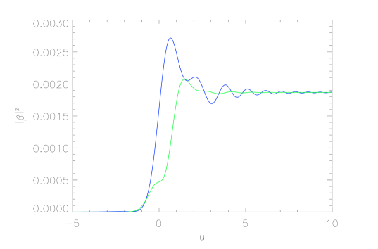
Figure 1: The mean number of particles created from the vacuum in state, given by (84) with $f_{\bf k}=f_{\lambda\,(+)}(u)$ of (56), and with $\lambda=1$. The blue curve with larger oscillations is for the choice of ($W_{\bf k},V_{\bf k}$) given by (85), while the green curve is for the second order adiabatic frequency of (86) and the same $V_{\bf k}$. Both change rapidly around $u=0$, and both tend to the same asymptotic value $e^{-2\pi}=0.001867$ of (88) as $u\rightarrow\infty$.

A continuous but sharp rise in $|\beta_{\bf k}|^{2}$ is observed in each $k_{z}$ mode around its ‘creation event,’ at $u=0$, i.e. at the time when the kinetic momentum $p=k_{z}+eEt=0$. Since the adiabatic mode functions are essentially WKB approximations to the time dependent harmonic oscillator equation (16) or (50), the particle creation process in real time and this rapid rise may be understood from a consideration of the WKB turning points in the complex $u$ plane PokKhal . These are defined by the values of $u$ where the frequency function $\omega_{\bf k}$ vanishes. Since the solutions are oscillatory on the real time axis, those turning points are located off the real line, and in the case of (50)-(51) these zeroes of the frequency are at

$$u=\pm u_{\lambda}\equiv\pm\,2i\,\sqrt{\lambda}$$ (87)

illustrated in Fig. 2.

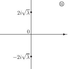
Figure 2: Location of the zeroes of the frequency function $\omega_{\bf k}$ in the complex $u$ plane. Particle creation occurs as the real time $u$ contour passes the imaginary axis at $u=0$ between the pair of these zeroes.

The qualitative behavior of the Bogoliubov coefficient $\beta_{\bf k}(t)$ along the real $u$ axis can be found by finding the lines of steepest descent of the adiabatic phase function $\Theta_{\lambda}(u)$ of (55) in the complex $u$ plane, as they emanate from $u_{\lambda}$ PokKhal . Far from the turning points, for $|u|\gg 2\sqrt{\lambda}$, the exact mode functions are well approximated by the adiabatic WKB mode function (74) and hence $|\beta_{\bf k}(t)|^{2}$ defined by (84) will be approximately constant. For $u\ll-|u_{\lambda}|<0$ the adiabatic vacuum is approximately the in vacuum discussed previously and $|\beta_{\bf k}(t)|^{2}$ is nearly zero if it is initialized so that $|\beta_{\bf k}(t_{0})|^{2}=0$. For $u\gg|u_{\lambda}|>0$, the adiabatic vacuum is approximately the out vacuum. Again $|\beta_{\bf k}(t)|^{2}$ will be approximately constant in this region and given approximately by the total Bogoliubov coefficient $B^{tot}_{\lambda}$ from in to out. In the region $u\in[-u_{\lambda},u_{\lambda}]$, as $u$ passes nearest the complex turning points (87), the exact mode function $f_{\bf k}(t)$ receives an increasing admixture of the negative frequency component, and $|\beta_{\bf k}|^{2}$ changes rapidly from its in to out value. This change in $|\beta_{\bf k}(t)|^{2}$ in this region of $\Delta u\sim 4\sqrt{\lambda}$ or $\Delta t\sim 2\sqrt{k_{\perp}^{2}+m^{2}}/eE$ around $u=0$ (closest to the complex zero of $\omega_{\bf k}$) is given by (68) or

$$\Delta|\beta_{\bf k}|^{2}=|B^{tot}_{\lambda}|^{2}=e^{-2\pi\lambda}$$ (88)

and can also be found from (55) by evaluating $\exp[-4\,{\rm Im}\,\Theta_{\lambda}(u_{\lambda})]$ PokKhal . We use the total Bogoliubov coefficient $B^{tot}_{\lambda}$ since the rise in $|\beta_{\bf k}|^{2}$ changes continuously in this region $u\in[-u_{\lambda},u_{\lambda}]$ between the two complex zeroes (87) with no constant value halfway between. The behavior of $|\beta_{\bf k}(u)|^{2}$ for various $\lambda$ is plotted in Fig. 3 showing the asymptotic value of the jump in particle number consistent with (88). Since this jump $|\beta_{\bf k}|^{2}$ occurs around $u=0$, the particle creation ‘event’ occurs at a different time $t=-k_{z}/eE$ for modes with different $k_{z}$.

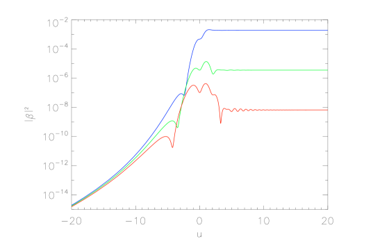
Figure 3: The mean number of particles created from the vacuum in state, given by (84) with $f_{\bf k}=f_{\lambda\,(+)}(u)$ of (56), and the second order adiabatic frequency of (86) for $\lambda=1,2,3$ (blue, green, red curves respectively). Note the logarithmic scale. The asymptotic values for large $u$ are $1.87\times 10^{-3}$, $3.49\times 10^{-6}$, and $6.51\times 10^{-9}$ for $\lambda=1,2,3$ respectively, in agreement with (88).

Consider now the adiabatic initial data at some finite time $t_{0}$,

$$f_{\bf k}(t_{0})=\frac{1}{\sqrt{2\omega_{\bf k}(t_{0})}}$$ (89a)

$$\frac{df_{\bf k}}{dt}\bigg{|}_{t=t_{0}}=-\left(i\omega_{\bf k}+\frac{\dot{\omega}_{\bf k}}{2\omega_{\bf k}}\right)f_{\bf k}\Big{|}_{t=t_{0}}$$ (89b)

with $\omega_{\bf k}(t)$ given by (51). This matches the adiabatic vacuum with (85) so that $\beta_{\bf k}(t_{0})=0$. Since the creation event occurs around $u=0=k_{z}+eEt$, with a finite starting time only those modes for which the initial kinetic momentum $p(t_{0})=k_{z}+eEt_{0}<0$ can experience this creation event. They do so at the time when their kinetic momentum $p(t)=k_{z}+eEt=0$, i.e. when the particle initially moving in the opposite direction to the electric field is brought to instantaneous rest $p(t)=0$ by the constant positive acceleration of the field and begins to move in the direction of the electric field. On the other hand those modes for which $p(t_{0})=k_{z}+eEt_{0}>0$ are already moving in the same direction of the electric field at the initial time and undergo no particle creation event at later times, being already approximately in the $\it out$ vacuum state at the initial time $t_{0}$. Crudely approximating the creation event as a step function at $u=0$ with step size (88), the number of particles in mode $\bf k$ at time $t>t_{0}$ is

$${\cal N}_{\bf k}(t) = (1+2N_{\bf k})|\beta_{\bf k}(t)|^{2}\approx\theta(p(t))\theta(-p(t_{0}))\,e^{-2\pi\lambda}$$ (90)

$$\approx (1+2N_{\bf k})\,\theta(k_{z}+eEt)\,\theta(-k_{z}-eEt_{0})\,e^{-2\pi\lambda}$$

where the factor of $1+2N_{\bf k}$ accounts for the induced creation rate of particles if there are already particles $N_{\bf k}>0$ in the initial state. From (90) there is a ‘window function’ in $k_{z}$ for modes going through particle creation given by

$$-eEt<k_{z}<-eEt_{0}$$ (91)

which grows linearly with elapsed time $t-t_{0}$. The behavior of $|\beta_{\bf k}|^{2}$ is shown in detail in Figs. 1 and 3, and Figures 2-4 of Ref. QVlas , with the $\theta$ functions actually smooth functions of $u$ that rise on the time scale of $\Delta u\sim 4\sqrt{\lambda}$, which can be accurately captured by the uniform asymptotic approximation of the parabolic cylinder functions even for moderately small $\lambda$ QVlas . Replacing this smooth rise of the average particle number by a step function already gives a qualitatively correct picture of the semi-classical particle creation process mode by mode in real time, with the correct asymptotic density of particles. It is the window function (91) which justifies the replacement of the integral over $k_{z}$ in (73) by $eE$ times the total elapsed time $T=t-t_{0}$, which can then be divided out to obtain the decay rate. The window function (91) of the real time particle creation process also agrees with the analysis of adiabatically switching on and off of the background electric field, so that it acts only for a finite time Nar ; NarNik ; GavGit ; AndMotSan . It is this definition of particles created by the electric field in the adiabatic basis that forms the starting point in quantum theory for a kinetic description QVlas .

The adiabatic basis also furnishes a simple physically well-motivated method for defining renormalized expectation values of current and energy-momentum bilinears in the quantum field. In the approximation in which the electric field background is treated classically while the charged scalar matter field is quantized, the renormalized $j_{z}$ current expectation value is

$$\langle t_{0}|j_{z}(t)|t_{0}\rangle_{{}_{R}}=2e\int\frac{d^{3}{\bf k}}{(2\pi)^{3}}\,(k_{z}+eEt)\left[(1+2N_{\bf k})|f_{\bf k}(t)|^{2}-\frac{1}{2\omega_{\bf k}(t)}\right]$$ (92)

where the leading divergence has been subtracted by the adiabatic vacuum term in which $|f_{\bf k}|^{2}$ has been replaced by $|\tilde{f}_{\bf k}|^{2}$ with (85) and $N_{\bf k}$ replaced by zero. It can be shown that this one subtraction removes all the UV divergences in the momentum integral for a constant $E$ field KESCM . A logarithmic divergence proportional to $\ddot{E}$ can be removed by using the second adiabatic order approximation for $W_{\bf k}$ in the expansion (77). As this term can easily be reabsorbed into coupling renormalization in backreaction calculations and vanishes in any case for a constant $E$ field, the lowest order subtraction in (92) is sufficient for our present purposes.

Substituting (75) we obtain from (92)

$$\langle t_{0}|j_{z}(t)|t_{0}\rangle_{{}_{R}}=2e\int\frac{d^{3}{\bf k}}{(2\pi)^{3}}\,\frac{(k_{z}+eEt)}{\omega_{\bf k}}\,\Big{[}\,{\cal N}_{\bf k}+{\rm Re}\,(\alpha_{\bf k}\beta^{*}_{\bf k}e^{-2i\Theta_{\bf k}})\,\Big{]}$$ (93)

where

$$\Theta_{\bf k}\equiv\int_{t_{0}}^{t}\omega_{\bf k}\,dt=\Theta_{\lambda}(u(t))-\Theta_{\lambda}(u(t_{0}))$$ (94)

is the adiabatic phase in (74), related to the function $\Theta_{\lambda}(u)$ defined in (55). Since $(k_{z}+eEt)/\omega_{\bf k}=p/\omega_{\bf k}$ is the $z$ component of the velocity of a classical particle in the electric field, the first term in the integral of (93) has a self-evident classical interpretation as the contribution to the electric current of the positive plus negatively charged particles with phase space number density ${\cal N}_{\bf k}$. The second term is a quantum interference term which has no classical analog. This term is both rapidly oscillating in time and rapidly oscillating in $|\bf k|$ for fixed time, so one would expect it to average out in the integral and give a relatively small contribution to the total current compared to the first term. For the semi-classical particle interpretation based on the adiabatic modes (74) to be most useful, this should be the case. If it is, one can also substitute the step approximation (90) for the particle density (assuming $N_{\bf k}=0$, i.e. no particles in the initial state) and arrive at the simple result

$$\langle t_{0}|j_{z}(t)|t_{0}\rangle_{{}_{R}} \approx 2e\int\frac{d^{3}{\bf k}}{(2\pi)^{3}}\,\frac{(k_{z}+eEt)}{\omega_{\bf k}(t)}\,\theta(k_{z}+eEt)\,\theta(-k_{z}-eEt_{0})\,\exp\left[-\frac{\pi(k_{\perp}^{2}+m^{2})}{eE}\right]$$ (95)

$$=\frac{e}{\pi}\,\Big{[}\sqrt{e^{2}E^{2}(t-t_{0})^{2}+m^{2}}-m\Big{]}\,\int_{0}^{\infty}\frac{dk_{\perp}^{2}}{4\pi}\,\exp\left[-\frac{\pi(k_{\perp}^{2}+m^{2})}{eE}\right]$$

$$\rightarrow\frac{e^{3}E^{2}}{4\pi^{3}}\,(t-t_{0})\,e^{-\frac{\pi m^{2}}{eE\ }}$$

for the linear growth with time of the mean electric current of the created particles. This exhibits the secular effect coming from the window function (91) opening linearly with time so that more and more modes go through their particle creation event as time goes on, each becoming accelerated very rapidly to the speed of light, and making a constant contribution to the current.

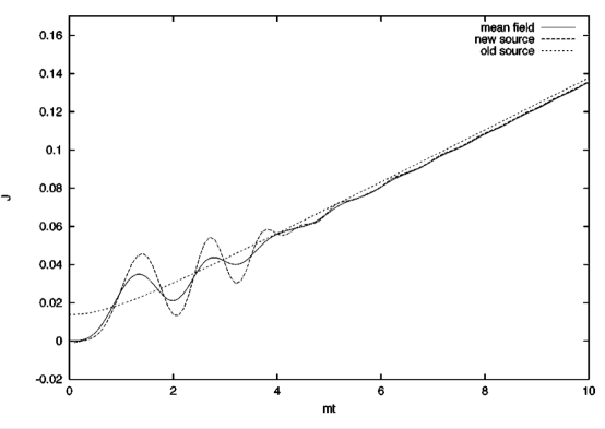
Figure 4: The linear growth of the electric current $J=\langle j_{z}\rangle$ with time in the case of fixed constant background electric field in $1+1$ dimensions in units of $e^{2}E$ for $eE/m^{2}=1$. The three curves shown are the current of the exact renormalized current expectation value (92), a uniform approximation described in Ref. QVlas (new source) and with the simple window step function of particle creation (90), (95), labelled old source here.

One can also evaluate the exact expectation value (92) for a constant uniform electric field background starting with the initial adiabatic data (89) and compare it to the simple step function approximation (95). This comparison is shown in Fig. 4 QVlas . The transient oscillations are the effect of the second quantum interference term in (93) while the dominant secular effect of linear growth at late times is correctly captured by the simple approximation (95) based on the particle creation picture, labelled as ‘old source’ in Fig. 4. The curve labeled ‘new source’ is the uniform approximation of QVlas that gives a slightly better approximation than the crude step function approximation of (90). Either gives correctly the coefficient of the linear secular growth with time, which implies that backreaction must eventually be taken into account, no matter how small $eE/m^{2}$ is, provided only that it is non-zero. This secular growth is a non-perturbative infrared ‘memory effect’ in the sense of depending upon the time elapsed since the initial vacuum state is prepared at $t=t_{0}$. Note that this time dependence due to particle creation is a spontaneous breaking of the time translational and time reversal symmetry of the background constant $\bf E$ field Fluc . The exponentially small tunneling factor associated with the spontaneous Schwinger particle creation rate from the vacuum shows that the effect is non-perturbative, but that however small, it can be overcome by a large initial state density of particles $N_{\bf k}>>1$ for which the induced particle creation and current is much larger. Even in the initial adiabatic vacuum case for $N_{\bf k}=0$, particle creation eventually overcomes the small tunneling factor at late times.

VI Adiabatic States and Initial Data in de Sitter Space

As in the electric field case, we introduce instantaneous adiabatic vacuum states in de Sitter space, defined by the adiabatic mode functions

$$\tilde{f}_{k}=\frac{1}{\sqrt{2W_{k}}}\,\exp\left(-i\int^{\tau}d\tau\,W_{k}\right)$$ (96)

analogous to (74). Due to spatial homogeneity and isotropy in the cosmological case, these modes depend only upon the magnitude $k=|{\bf k}|$ which is the principal quantum number of the spherical harmonic on ${\mathbb{S}}^{3}$. The time dependent coefficients $\alpha_{k}(u)$ and $\beta_{k}(u)$ of the Bogoliubov transformation are defined by

$$f_{k} = \alpha_{k}\tilde{f}_{k}+\beta_{k}\tilde{f}_{k}^{*}$$ (97a)

$$H\frac{d}{du}f_{k} = \left(-iW_{k}+\frac{V_{k}}{2}\right)\alpha_{k}\tilde{f}_{k}+\left(iW_{k}+\frac{V_{k}}{2}\right)\beta_{k}\tilde{f}_{k}^{*}$$ (97b)

where $f_{k}$ is an exact mode function solution of (16). They are given again by (83), viz.

$$|\beta_{\bf k}(t)|^{2}=\frac{1}{2W_{\bf k}}\left|\dot{f}_{\bf k}+\left(iW_{\bf k}-\frac{V_{\bf k}}{2}\right)f_{\bf k}\right|^{2}$$ (98)

and (76) is satisfied, provided only that both $W_{k}$ and $V_{k}$ are arbitrary real functions of time.

The analog of (75) is now

$$\left(\begin{array}[]{c}\tilde{a}_{klm_{l}}(u)\\ \tilde{a}_{kl\,-m_{l}}^{{\dagger}}(u)\end{array}\right)=\left(\begin{array}[]{cc}\alpha_{k}(u)&\beta_{k}^{*}(u)\\ \beta_{k}(u)&\alpha_{k}^{*}(u)\end{array}\right)\ \left(\begin{array}[]{c}a_{klm_{l}}\\ a^{{\dagger}}_{kl\,-m_{l}}\end{array}\right)$$ (99)

when referred to any time independent basis $(a_{klm_{l}},a^{{\dagger}}_{kl\,-m_{l}})$ for the Hermitian scalar field $\Phi$ (not necessarily the CTBD basis). The time dependent mean adiabatic particle number in the mode $(klm_{l})$ is independent of $(lm_{l})$ for $O(4)$ invariant adiabatic states and may be defined by the analog of (81) in de Sitter space to be

$${\cal N}_{k}(u)=\langle\tilde{a}^{{\dagger}}_{klm_{l}}(u)\tilde{a}_{klm_{l}}(u)\rangle=N_{k}+(1+2N_{k})|\beta_{k}(u)|^{2}$$ (100)

where

$$N_{k}\equiv\langle a^{{\dagger}}_{klm_{l}}a_{klm_{l}}\rangle$$ (101)

is the number of particles at the initial time $u=u_{0}$, provided $|\beta_{\bf k}(u_{0})|^{2}=0$ is initialized to zero at the initial time $u=u_{0}$. Note that with this initialization, the exact mode function solution of (16) satisfies the initial conditions

$$f_{k\gamma}(u_{0})=\frac{1}{\sqrt{2W_{k}}}\bigg{|}_{u=u_{0}}\,,\qquad\dot{f}_{k\gamma}(u_{0})=\frac{1}{\sqrt{2W_{k}}}\left(-iW_{k}+\frac{V_{k}}{2}\right)\bigg{|}_{u=u_{0}}$$ (102)

and hence is a certain linear combination (time independent Bogoliubov transformation) of the CTBD mode function $F_{k\gamma}$ and its complex conjugate $F_{k\gamma}^{*}$. Correspondingly, the time independent basis operators $a_{klm_{l}},a_{klm_{l}}^{{\dagger}}$ in Fock space are certain linear combinations of the $a^{\upsilon}_{klm_{l}},a^{\upsilon\,{\dagger}}_{klm_{l}}$ operators that define the de Sitter invariant state (14), which can be expressed in terms of each other by time independent Bogoliubov coefficients dependent upon the initial data (102).

As in the electric field example, the behavior of the solutions of the mode equation (16) can be analyzed by general WKB methods in the complex $u$ plane. The zeroes of the frequency function, $\Omega_{k}=0$ in (18) occur at the complex values $\cosh\bar{u}=\pm i\,\gamma^{-1}\sqrt{k^{2}-1/4}$, or

$$\hskip 19.91692pt\bar{u}=u_{R}+iu_{I}=\pm u_{k\gamma}+i\pi\left(n+\tfrac{1}{2}\right)\quad{\rm with}\quad n\in\mathbb{Z}\quad{\rm and}$$ (103a)

$$\sinh u_{k\gamma}=\frac{\sqrt{k^{2}-\frac{1}{4}}}{\gamma}\,,\qquad u_{k\gamma}=\ln\left[\frac{\sqrt{k^{2}-\frac{1}{4}}+\sqrt{\gamma^{2}+k^{2}-\frac{1}{4}}}{\gamma}\right]\;.$$ (103b)

Thus there is an infinite line of zeroes of $\Omega_{k}$ in the complex $u$ plane along the two vertical axes at $u=\pm u_{k\gamma}$ for $\gamma^{2}>0$, c.f. Fig. 5. The largest effect on the Bogoliubov coefficient $\beta_{k}(u)$ will occur when the real time contour passes closest to these lines of complex turning points at $u=\pm u_{k\gamma}$. Hence there are two ‘creation events’ in global de Sitter space, one in the contracting and one in the expanding phase symmetric around $u=0$.

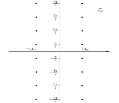
Figure 5: Location of the zeroes (103) of the frequency function $\Omega_{k}$ (17) in the complex $u$ plane for $\gamma^{2}>0$. Particle creation occurs as the real time $u$ contour passes through the lines of these zeroes at $u=\mp u_{k\gamma}$.

We may consider the two limits

$$\hskip 28.45274ptu_{k\gamma}\rightarrow\frac{\sqrt{k^{2}-\frac{1}{4}}}{\gamma}\rightarrow 0\quad{\rm for}\quad\gamma\gg k\,;\qquad{\rm or}$$ (104a)

$$u_{k\gamma}\rightarrow\ln\left(\frac{2\sqrt{k^{2}-\frac{1}{4}}}{\gamma}\right)\rightarrow\ln\left(\frac{2k}{\gamma}\right)\rightarrow\infty\quad{\rm for}\quad k\gg\gamma\,.$$ (104b)

The first limit (104a) is the non-relativistic limit of very heavy particles whose rest mass is much larger than their physical momentum $k/a$ at all times. These non-relativistic particles are created nearly at rest close to the symmetric point $u=0$ between the contracting and expanding de Sitter phases, so that the two events merge into one. The second limit (104b) is the relativistic limit of particles whose physical momentum is much larger than their rest mass for most of their history. These particles are created in two bursts, at $u=\mp u_{k\gamma}$, when their physical momentum $kH\,{\rm sech}\,u_{k\gamma}$ is of the same order as their rest mass, so that they are moderately relativistic at creation. In the contracting phase of de Sitter space $u<0$ these particles, created around $u=-u_{k\gamma}$, are blueshifted exponentially rapidly in $u$, and thus become ultrarelativistic. This contracting phase with the created particles becoming ultrarelativistic is therefore most analogous to the previous electric field example, and is the phase where we can expect the largest backreaction effects. Conversely, in the expanding phase, $u>0$, the particles created around $u=+u_{k\gamma}$ will be subsequently exponentially redshifted in $u$, and therefore have a much smaller backreaction effect. We emphasize that the time $\pm u_{k\gamma}$ is of the order of the horizon crossing of the mode at $u\sim\pm\ln(2k)$ only for $\gamma\sim 1$. For large $\gamma\gg k$ the particle creation events occur when the wavelength of the mode is much smaller than the horizon, while for $\gamma\rightarrow 0$ the particle creation events occur when the wavelength of the mode is much greater than the horizon. Due to the different disposition of zeroes of the adiabatic frequency in the electric field and de Sitter cases, c.f. Figs. 2 and 5, there is no analog of this second burst of particle creation in the electric field case.

For moderate values of $\gamma$, most of the $k$ modes fall into the second case (104b), and experience two well-separated creation events at large $u_{k\gamma}\gg 1$ in both the contracting and expanding phases of de Sitter space. In contrast to the electric field case considered previously we may therefore distinguish three distinct regions:

$$I:\qquad u<-u_{k\gamma}\,,\qquad\qquad\quad in$$ (105a)

$$II:\quad-u_{k\gamma}<u<u_{k\gamma}\,,\qquad CTBD$$ (105b)

$$III:\quad u_{k\gamma}<u\,,\qquad\qquad\quad\ \ out$$ (105c)

where we have indicated the character of the adiabatic vacuum in each region. If one takes the infinite time limits $u\rightarrow\mp\infty$ with $k$ and $\gamma$ and hence $u_{k\gamma}$ fixed, one is automatically in the first in region or the third out region respectively. This corresponds to the in/out scattering problem considered in Sec. III. If on the other hand one takes the $k\rightarrow\infty$ limit for fixed $u,\gamma$ then Eq. (104b) shows that one is always in region II, where the CTBD state is the adiabatic vacuum. This shows explicitly the non-commutivity of the infinite $u$ and infinite $k$ limits, with the transition between the two limits occurring at $u=\pm u_{k\gamma}$.

Next we consider the mode function(s) and adiabatic vacuum state specified by the initial values (102) at an arbitrary finite time $u_{0}<0$. The modes for a given value of $k$ fall into two possible classes:

$$(i) \ -u_{k\gamma}<u_{0}<0$$ (106a)

$$(ii) \ u_{0}<-u_{k\gamma}<0\,.$$ (106b)

For modes in the first class (i) the initial time $u_{0}$ is already later than the first creation event. For these modes in region II, the adiabatic initial condition is close to the CTBD state in the high $k$ limit, $\beta_{k}\approx 0$ and nothing further happens in the contracting phase, as they remain in region II for all $u_{0}<u\leq 0$. In contrast, the $k$ modes in class (ii) are approximately in the in vacuum state initially. These modes have yet to go through their particle creation event which occurs at the later time $u=-u_{k\gamma}>u_{0}$ in the contracting phase. At that time, the adiabatic particle vacuum switches rapidly to approximately the CTBD state as $u$ increases past $-u_{k\gamma}$. Thus this mode sees its time dependent Bogoliubov coefficient change rapidly in a few expansion times ($\Delta u\sim 1$ since the imaginary part of the nearest complex zero of $\Omega_{k}$ is $\pi/2$ and independent of $k,\gamma$) from approximately zero to a non-zero plateau determined by the Bogoliubov coefficient (34b). Approximating the jump in particle number at these creation events by a step function as before, we have

$$\Delta|\beta_{k}|^{2}=|B^{in}_{k\gamma}|^{2}=\frac{e^{-\pi\gamma}}{2\sinh(\pi\gamma)}=\frac{1}{e^{2\pi\gamma}-1}$$ (107a)

$${\cal N}_{k}(u)\approx\theta(u+u_{k\gamma})\ \theta(-u_{k\gamma}-u_{0})\,\Delta{\cal N}_{1,k\gamma}\quad{\rm for}\quad u<0\,,\quad u_{0}<0$$ (107b)

$$\quad\Delta{\cal N}_{1,k\gamma}=(1+2N_{k})\,\Delta|\beta_{k}|^{2}=\frac{1+2N_{k}}{e^{2\pi\gamma}-1}$$ (107c)

in the contracting phase. The first $\theta$ function in (107) specifies the time of the creation event when the step occurs, while the second $\theta$ function restricts the modes to class (ii) for which the step occurs at a later time $u=-u_{k\gamma}>u_{0}$ in the contracting phase. These two $\theta$ functions give the ‘window function’ which is similar to that found in the electric field case (91), namely

$$K_{\gamma}(u)\equiv\sqrt{\gamma^{2}\sinh^{2}u+\tfrac{1}{4}}<k<\sqrt{\gamma^{2}\sinh^{2}u_{0}+\tfrac{1}{4}}=K_{\gamma}(u_{0})$$ (108)

in the contracting phase of de Sitter space for which $u_{0}<u\leq 0$. Like (91) this window function has an upper limit fixed by the initial time and a lower limit which decreases as time evolves (for $u<0$).

If we continue the evolution past the symmetric point $u=0$ into the expanding de Sitter phase, all of the modes of class (ii) have experienced the first particle creation event, and then begin (with the smallest value of $k$ first) to experience a second creation event at $u=+u_{k\gamma}$. Thus the modes of class (ii) which started in region I undergo two creation events with a total Bogoliubov transformation of (35), while the modes of class (i) which started in region II undergo only the second creation event in the expanding phase for which the single Bogoliubov transformation $B_{k\gamma}^{out}$ applies. Again approximating these creation events by step functions we obtain

$${\cal N}_{k}(u)\approx\left[\theta(u_{k\gamma}-u)\,\theta(-u_{k\gamma}-u_{0})+\theta(u-u_{k\gamma})\theta(u_{0}+u_{k\gamma})\right]\,\Delta{\cal N}_{1,k\gamma}$$

$$\qquad+\,\theta(u-u_{k\gamma})\,\theta(-u_{k\gamma}-u_{0})\,\Delta{\cal N}_{2,k\gamma}\quad{\rm for}\quad u>0\,,\quad u_{0}<0$$ (109a)

$$\hskip 42.67912pt\Delta{\cal N}_{2,k\gamma}=(1+2N_{k})\,|B_{k\gamma}^{tot}|^{2}=(1+2N_{k})\,{\rm csch}^{2}(\pi\gamma)$$ (109b)

in the expanding phase of de Sitter space. The window function for this second creation event in the expanding phase is now

$$k<\sqrt{\gamma^{2}\sinh^{2}u+\frac{1}{4}}=K_{\gamma}(u)$$ (110)

for the modes undergoing the second creation event at $u=+u_{k\gamma}$. Those with $k<K_{\gamma}(u_{0})$ undergo both the first and second creation events with $\Delta{\cal N}=\Delta{\cal N}_{2,k\gamma}$, while those with $k>K_{\gamma}(u_{0})$ experience only the second creation event with $\Delta{\cal N}=\Delta{\cal N}_{1,k\gamma}$.

This analysis may be repeated if the initial time $u_{0}>0$ is in the expanding phase. In this case all modes initially in region II, with $u_{0}<u_{k\gamma}$ undergo a single creation event at $u=+u_{k\gamma}$. Hence we have

$${\cal N}_{k}(\tau)\approx\theta(u-u_{k\gamma})\,\theta(u_{k\gamma}-u_{0})\,\Delta{\cal N}_{1,k\gamma}\quad{\rm for}\quad u,\ u_{0}>0$$ (111)

replacing (109a). The window function in $k$ is now the reverse of (108), namely

$$K_{\gamma}(u_{0})<k<K_{\gamma}(u)$$ (112)

which like (110) shows an upper limit that increases with time.

The various cases (107), (109a) and (111) may be collected into one result

$${\cal N}_{k}(\tau)\approx\Big{[}\theta(u_{k\gamma}-|u|)\ \theta(-u_{k\gamma}-u_{0})+\theta(u-u_{k\gamma})\ \theta(u_{k\gamma}-|u_{0}|)\Big{]}\,\left(\frac{1+2N_{k}}{e^{2\pi\gamma}-1}\right)$$

$$\hskip 56.9055pt+\ \theta(u-u_{k\gamma})\,\theta(-u_{k\gamma}-u_{0})\,(1+2N_{k})\,{\rm csch}^{2}(\pi\gamma)$$ (113)

valid for all values of $u$ and initial times $u_{0}$. From this or (109a) it is clear that for fixed $k$, with $u_{0}\rightarrow-\infty,u\rightarrow+\infty$, the mode experiences both particle creation events and we recover (36), while for a finite interval of time only those modes for which $u_{0}<-u_{k\gamma}$ and $u_{k\gamma}<u$ experience both creation events. Thus taking the symmetric limit with $u=-u_{0}>0$, the values of $k$ satisfying both these conditions are cut off at the maximum value $K_{\gamma}(u)$, i.e.

$$k\leq K_{\gamma}(u)\rightarrow\frac{\gamma}{2}\,e^{|u|}\qquad{\rm or}\qquad\ln K_{\gamma}(u)\rightarrow|u|+\ln\left(\frac{\gamma}{2}\right)$$ (114)

as $|u|\rightarrow\infty$, which is exactly the cutoff (42) that we argued on physical grounds earlier in Sec. III (and in Ref. PartCreatdS ) should be used in the $k$ sum of (38) to calculate the finite decay rate per unit volume (46) of de Sitter space to massive particle creation in the limit $V_{4}\rightarrow\infty$. The constant in (42) has been determined to be $\ln(\gamma/2)$ by our detailed analysis of the particle creation process in real time. The non-Hadamard short distance behavior of the in and out states found in PartCreatdS has also been removed by regulating the large $k$ behavior with a finite initial and final time, since the modes for which $k>K_{\gamma}(u)$ remain in the CTBD state in region II for all $-|u_{0}|<u<|u_{0}|$ and the CTBD state is known to have the correct short distance behavior BunDav .

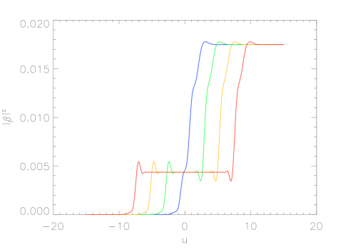
Figure 6: Pllotted is $|\beta_{k}(u)|^{2}$ for $m=H$ defined by (98) with the initial adiabatic matching time $u_{0}=-15$ and the second order matching defined by (115). The innermost blue curve is for $k=1$, the green for $k=10$, the yellow for $k=100$ and the outermost red for $k=1000$, the latter $3$ values showing two clearly separated particle creation events. The values of $u_{k\gamma}$ given by (103) are $0.35$, $2.31$, $5.44$, and $10.0$ respectively for these values of $k$ and $\gamma$. The asymptotic value of $|\beta_{k}|^{2}$ of all the curves for large $u$ is $0.01748$ in agreement with (109b) for $N_{k}=0$. The intermediate plateau is at $0.00435$ in agreement with (107c).

The actual smooth behaviors of $|\beta_{k}(u)|^{2}$ defined by (98) for various $k$ and $u_{0}=-15$ and $u_{0}=-5$ are shown in Figs. 6 and 7 respectively. The increases in $|\beta_{k}(u)|^{2}$ occur on a time scale $\Delta u\sim 1$ for all the modes. The values chosen for the adiabatic frequency functions $(W_{k},V_{k})$ are

$$W_{k}^{(2)}=\Omega_{k}+\frac{3}{8}\frac{\dot{\omega}_{k}^{2}}{\omega_{k}^{3}}-\frac{1}{4}\frac{\ddot{\omega}_{k}}{\omega_{k}^{2}}$$

$$\qquad=\Omega_{k}+\frac{h^{2}}{8\,\omega_{k}}\left(1-\frac{6m^{2}}{\omega_{k}^{2}}+\frac{5m^{4}}{\omega_{k}^{4}}\right)+\frac{\dot{h}}{4\,\omega_{k}}\left(1-\frac{m^{2}}{\omega_{k}^{2}}\right)\,,$$ (115a)

$$V_{k}^{(1)}=-\frac{\dot{\omega}_{k}}{\omega_{k}}=h\left(1-\frac{m^{2}}{\omega_{k}^{2}}\right)$$ (115b)

correct up to second order in the adiabatic expansion. A comparison of $|\beta_{k}(u)|^{2}$ for this choice and the simpler choice

$$W_{k}^{(0)}=\Omega_{k}=H\left[\left(k^{2}-\tfrac{1}{4}\right){\rm sech}^{2}u+\gamma^{2}\right]^{\frac{1}{2}}$$ (116a)

$$V_{k}^{(1)}=-\frac{\dot{\omega}_{k}}{\omega_{k}}=h\left(1-\frac{m^{2}}{\omega_{k}^{2}}\right)$$ (116b)

for the $k=10$ mode and $u_{0}=-15$ is shown in Fig. 8.

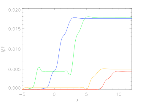
Figure 7: Plotted is $|\beta_{k}(u)|^{2}$ for the same values of $\gamma$ and $k$ as in Fig. 7, but with the initial adiabatic matching time $u_{0}=-5$. Note that for the two highest values of $k$ at $100$ and $1000$ (the lower yellow and red curves), a marked first particle creation event does not occur since $u_{0}>-u_{k\gamma}$ for these modes. The asymptotic value of the lower red curve at large $u$ is $0.00435$ in agreement with the first term of (113). The yellow curve for $k=100$ has a small contribution from the first creation event since $u_{0}$ and $-u_{k\gamma}$ are comparable.

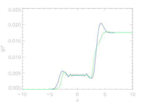
Figure 8: Plotted is $|\beta_{k}(u)|^{2}$ for $k=10$ when the matching time is $u_{0}=-15$. The blue curve corresponds to the zeroth order adiabatic vacuum state specified by $W_{k}=\Omega_{k}$ with $V_{k}$ given by (116). The green curve corresponds to the second order adiabatic vacuum state specified by (115).

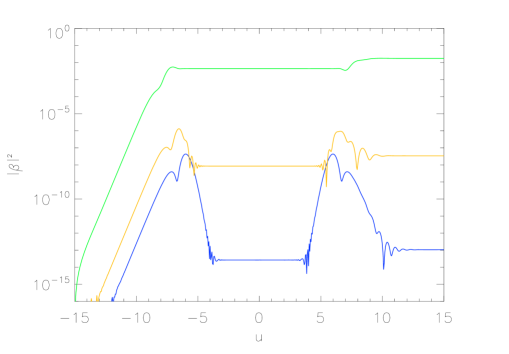
Figure 9: Plotted is $|\beta_{k}(u)|^{2}$ for fixed $k=1000$ and adiabatic matching time $u_{0}=-15$, for three values of the mass: $m=H$ (upper, green), $m=3H$ (middle, yellow), $m=5H$ (lower, blue). Note the logarithmic scale. The asymptotic values of $|\beta_{k}|^{2}$ for large $u$ are $1.748\times 10^{-2},3.391\times 10^{-8}$ and $1.062\times 10^{-13}$ respectively, in agreement with (109b) for $N_{k}=0$. The intermediate plateaux at $u=0$ are at $4.35\times 10^{-3},8.48\times 10^{-9}$, and $2.66\times 10^{-14}$ respectively, in agreement with (107c). The particle creation events occur at $\mp u_{k\gamma}$ with $u_{k\gamma}=7.74,6.52$ and $6.00$ respectively for the three values of $m$.

As in the electric field case (c.f. Fig. 1) the detailed time structure of the creation event is different with different choices of $(W_{k},V_{k})$, but the qualitative features and asymptotic values (and intermediate plateau value) are independent of the choice. The second order WKB choice (115) suppresses the oscillations observed with the choice (116) and comes closer to the approximate step function description. As predicted by the previous WKB analysis and (113), the modes with $k=1$ and $k=10$ in Fig. 7 go through both creation events with a rapid increase in $|\beta_{k}(u)|^{2}$ occurring for each at the appropriate value of $\mp u_{k\gamma}$. The modes with $k=100$ and $k=1000$ for which $u_{k\gamma}>|u_{0}|$ only go through a marked second creation event, although the yellow curve for $k=100$ has a small contribution from the first creation event, since $u_{0}=-5$ and $-u_{k\gamma}=-5.44$ are comparable for this mode. The value of $|\beta_{k}(u)|^{2}$ after the first creation event is well approximated by (107a) or (107c) with $N_{k}=0$ for an initial vacuum, while for those modes undergoing two creation events the second plateau of $|\beta_{k}(u)|^{2}$ for $u>u_{k\gamma}$ is given by (109b). In Fig. 9 we also compare $|\beta_{k}(u)|^{2}$ for fixed $k=1000$ and $u_{0}=-15$, for three different values of the mass, showing the dependence of the time of the creation events on $\gamma$ given by (103b).

For comparison we also plot the adiabatic particle number as a function of $u$ for the CTBD state in Fig. 10. This figure shows that the CTBD state contains particles in its initial condition and the first event at $u=-u_{k\gamma}$ is actually a particle destruction event. The phase coherent initial particles in modes with principal quantum number $k$ find each other and annihilate at the time $u=-u_{k\gamma}$, canceling each other precisely in region II. At the later time $u=u_{k\gamma}$ these particles are created again in a completely time symmetric manner. This is clearly a delicately balanced coherent process that is artificially arranged by initial conditions in the CTBD state. In an accompanying paper we show that a small perturbation of the CTBD state upsets this balance and leads again to instability AndMotDSVacua .

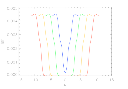
Figure 10: Plotted is $|\beta_{k}(u)|^{2}$ for the CTBD state for various values of $k$: $k=1$ (blue), $k=10$ (green). $k=100$ (orange), $k=1000$ (red). Note that the first event at $u=-u_{k\gamma}$ is a particle annihilation event in which the particle number decreases from $0.004352$ to zero in each $k$ mode, rising again to the same value at $u=+u_{k\gamma}$ in a completely time symmetric manner.

VII Particle Creation in Spatially Flat FLRW Poincaré Coordinates

The analysis of particle creation in the spatially closed ${\mathbb{S}}^{3}$ coordinates of de Sitter space of the previous section can just as well be carried out in the spatially flat Poincaré coordinates of (161), more commonly used in cosmology. The wave equation (1) again separates in the usual Fourier basis $\Phi\sim\phi_{k}(\tau)e^{i{\bf k\cdot x}}$. Removing the scale factor by defining the mode function $f_{k}=a^{\frac{3}{2}}\phi_{k}$ as in (15) but with $a=\exp(H\tau)$ in this case gives the mode equation

$$\left[\frac{d^{2}}{d\tau^{2}}+k^{2}e^{-2H\tau}+m^{2}-\frac{H^{2}}{4\,}\right]f_{k}(\tau)=0$$ (117)

with $k\equiv|\bf k|$. This equation again has the form of an harmonic oscillator equation with a time dependent frequency which is given by

$$\omega_{k}^{2}(\tau)=k^{2}e^{-2H\tau}+m^{2}-\frac{H^{2}}{4\,}\;.$$ (118)

Thus with this change all of the methods employed in the spatially closed sections or the electric field background may be utilized again. In particular, for $\gamma^{2}>0$ we have over the barrier scattering in a non-trivial one dimensional potential, and we should expect the stationary waves incident from the left as $\tau\rightarrow-\infty$ to be partially reflected and partially transmitted to the right as $\tau\rightarrow\infty$. This scattering will result again in a non-trivial Bogoliubov transformation between the positive frequency particle solutions at early times in the in vacuum and those at late times in the out vacuum, i.e. particle creation, just as in the electric field case.

By making the change of variables

$$z\equiv\frac{k}{H}\,e^{-H\tau}$$ (119)

Eq. (117) may be transformed into Bessel’s equation with imaginary index $\nu=\pm i\gamma$. Thus the exact solutions are Bessel or Hankel functions with this index. The particular solution

$$\bar{\upsilon}_{\gamma}(z)\equiv\frac{1}{2}\sqrt{\frac{\pi}{H}}\,e^{-\frac{\pi\gamma}{2}}e^{\frac{i\pi}{4}}H^{(1)}_{i\gamma}(z)=\sqrt{\frac{\pi}{H}}\,\frac{e^{\frac{\pi\gamma}{2}}e^{\frac{i\pi}{4}}}{e^{2\pi\gamma}-1}\,\Big{[}e^{\pi\gamma}J_{i\gamma}(z)-J_{-i\gamma}(z)\Big{]}$$ (120)

is the CTBD solution in flat coordinates, with the asymptotic behavior

$$\bar{\upsilon}_{\gamma}(z)\rightarrow\frac{1}{\sqrt{2Hz}}\,e^{iz}\qquad{\rm as}\qquad z\rightarrow\infty\,.$$ (121)

Since $\omega_{k}=H\sqrt{z^{2}+\gamma^{2}}\rightarrow Hz$ and

$$\Theta_{\gamma}(z) \equiv \int^{\tau(z)}\,d\tau\,\omega_{k}(\tau)=-\int^{z}\frac{dz}{z}\sqrt{z^{2}+\gamma^{2}}$$ (122)

$$= -\sqrt{z^{2}+\gamma^{2}}-\frac{\gamma}{2}\ln\left[\frac{\sqrt{z^{2}+\gamma^{2}}-\gamma}{\sqrt{z^{2}+\gamma^{2}}+\gamma}\right]\rightarrow-z\qquad{\rm as}\qquad z\rightarrow\infty$$

the solution (120) is also the correctly normalized adiabatic in vacuum solution

$$f_{k(+)}(\tau)=\bar{\upsilon}_{\gamma}(z)\rightarrow\frac{1}{\sqrt{2\omega_{k}}}\,e^{-i\Theta_{\gamma}}\qquad{\rm as}\qquad\tau\rightarrow-\infty$$ (123)

in the Poincaré coordinates.

This much is standard and may be found in standard references BirDav . However, in the opposite limit of late times $\tau\rightarrow\infty$

$$\omega_{k}\rightarrow H\gamma\qquad{\rm and}\qquad\Theta_{\gamma}(z)\rightarrow-\gamma\ln z\qquad{\rm as}\qquad z\rightarrow 0$$ (124)

and therefore

$$f_{k}^{(+)}(\tau)=\left(\frac{2H}{k}\right)^{i\gamma}\frac{\Gamma(1+i\gamma)}{\sqrt{2H\gamma}}\,J_{i\gamma}(z)\rightarrow\left(\frac{H}{k}\right)^{i\gamma}\frac{z^{i\gamma}}{\sqrt{2H\gamma}}=\frac{1}{\sqrt{2H\gamma}}\,e^{-i\gamma H\tau}\quad{\rm as}\quad\tau\rightarrow\infty$$ (125)

is the properly normalized positive frequency out solution, which agrees with the adiabatic form $e^{-i\Theta_{\gamma}}/\sqrt{2\omega_{k}}$ at late times. Comparison with the last form of (120) shows that indeed there is a nontrivial mixing of positive and negative frequencies at late times in the CTBD state. The Bogoliubov coefficients are

$$A_{\gamma}=\frac{\sqrt{2\pi\gamma}\ e^{\frac{i\pi}{4}}}{2^{i\gamma}\,\Gamma(1+i\gamma)}\ \frac{e^{\frac{3\pi\gamma}{2}}}{e^{2\pi\gamma}-1}$$ (126a)

$$B_{\gamma}=-\frac{\sqrt{2\pi\gamma}\ e^{\frac{i\pi}{4}}}{2^{i\gamma}\,\Gamma(1+i\gamma)}\ \frac{e^{\frac{\pi\gamma}{2}}}{e^{2\pi\gamma}-1}$$ (126b)

with $|A_{\gamma}|^{2}-|B_{\gamma}|^{2}=1$. Note that

$$|B_{\gamma}|^{2}=\frac{1}{e^{2\pi\gamma}-1}=|B^{out}_{k\gamma}|^{2}\;.$$ (127)

Thus $B_{k}$ has exactly the same magnitude as the corresponding Bogoliubov coefficient Eq.  (34b) obtained previously in the closed ${\mathbb{S}}^{3}$ spatial sections. This equality is to be expected since in the asymptotic future the closed spatial sections have negligible spatial curvature and there is no local difference with the flat sections. This mode mixing and particle creation effect in the flat Poincaré coordinates, which follows from the second form of (120), seems to have been overlooked in BirDav , which states that “there is no particle production.”

The particle creation process may be analyzed in real time in the flat Poincaré coordinates by using the methods of Sec. V. Indeed the zeroes of (118) in the complex $z$ plane occur at

$$z_{\gamma}=\pm i\gamma$$ (128)

which represents an infinite series of zeroes at $H\tau=\ln(k/H\gamma)+i\pi(n+\frac{1}{2})$ similar to those in the complex $u$ plane in Eq. (103) and Fig. 5. Since the Poincaré coordinates cover only one half of the de Sitter manifold, where it is only expanding (or in the other half where it is only contracting), there is only one line of complex zeroes in Poincaré coordinates and only one creation event occurring at

$$\tau_{k\gamma}=\frac{1}{H}\ln\left(\frac{k}{H\gamma}\right)$$ (129)

for the mode with Fourier component $k=|{\bf k}|$. If one starts the evolution at some finite initial time $\tau_{0}$ then only those modes with $k$ in the range determined by

$$\tau_{0}<\tau_{k\gamma}<\tau$$ (130)

will experience their creation event at a later time $\tau$. The number density of particles in modes with $k=|{\bf k}|$ at time $\tau$ is therefore

$${\cal N}_{k}(\tau)\approx\theta(\tau_{k\gamma}-\tau_{0})\,\theta(\tau-\tau_{k\gamma})\,(1+2N_{k})\,|B_{\gamma}|^{2}$$ (131)

in the approximation that the particles are created instantaneously when $\tau$ passes through $\tau_{k\gamma}$.

In the expanding phase of de Sitter space, whether described by closed ${\mathbb{S}}^{3}$ or flat ${\mathbb{R}}^{3}$ spatial sections, these particles will be redshifted in energy and make a decreasing contribution to the energy density and pressure at later times. In the next section we compute the energy density of the created particles which grow exponentially in the contracting part of de Sitter space due to their blueshifting toward the extreme ultrarelativistic limit. This does not occur in the Poincaré sections with only monotonic expansion, for spatially homogeneous states. In Attract we showed that the energy density and pressure relax to the values of the de Sitter invariant CTBD state for all such UV allowed spatially homogeneous states and for all $M^{2}>0$ in the expanding phase. Nevertheless the same particle creation and vacuum instability effect (or more precisely one half of it) is present in the Poincaré coordinates as in the closed section coordinates of the full hyperboloid. Spatially inhomogeneous states have a different behavior and are studied in AndMotDSVacua .

VIII Stress-Energy Tensor of Created Particles

In this section we consider the stress-energy tensor of the created particles, and their ability to affect the background de Sitter spacetime by backreaction. The energy-momentum tensor of the scalar field with arbitrary curvature coupling $\xi$ is

$$T_{ab}=(\nabla_{a}{\bf\Phi})(\nabla_{b}{\bf\Phi})-\frac{g_{ab}}{2}(\nabla^{c}{\bf\Phi})(\nabla_{c}{\bf\Phi})-\frac{m^{2}}{2}g_{ab}{\bf\Phi}^{2}+\xi\big{[}g_{ab}\,\raise 0.5pt\hbox{$\vbox{\hrule\hbox{\vrule height=6.50403pt\kern 6.50403pt\vrule} \hrule}$}\,-\nabla_{a}\nabla_{b}+G_{ab}\big{]}{\bf\Phi}^{2}$$ (132)

where $G_{ab}$ is the Einstein tensor. Assuming a metric of the form (2) and spatial homogeneity and isotropy of the state on the ${\mathbb{S}}^{3}$ sections, the only non-vanishing components of the expectation value of $T_{ab}$ are the energy density $\varepsilon=\langle T_{\tau\tau}\rangle$ and the isotropic pressure $p=\frac{1}{3}\langle T^{i}_{\ i}\rangle$. The scalar field operator $\bf\Phi$ can be expressed in terms of the exact mode function solutions of (16) such that

$${\bf\Phi}(u,\hat{N})=a^{-\frac{3}{2}}\sum_{k=1}^{\infty}\sum_{l=0}^{k-1}\sum_{m_{l}=-l}^{l}\left\{a_{klm_{l}}\,f_{k}(u)\,Y_{klm_{l}}(\hat{N})+a_{klm_{l}}^{\dagger}f^{*}_{k}(u)Y_{klm_{l}}^{*}\,(\hat{N})\right\}\;.$$ (133)

Assuming the mode functions satisfy the arbitrary initial conditions (102), and specializing to conformal coupling $\xi=\frac{1}{6}$, we find

$$\varepsilon\big{|}_{\xi=\frac{1}{6}} = \frac{1}{4\pi^{2}a^{3}}\sum_{k=1}^{\infty}\,(1+2N_{k})\left[|\dot{f}_{k}|^{2}-h\,{\rm Re}(f_{k}^{*}\dot{f}_{k})+\left(\frac{k^{2}}{a^{2}}+m^{2}+\frac{h^{2}}{4\,}\right)|f_{k}|^{2}\right]$$ (134a)

$$p\big{|}_{\xi=\frac{1}{6}} = \frac{1}{12\pi^{2}a^{3}}\sum_{k=1}^{\infty}\,(1+2N_{k})\left[|\dot{f}_{k}|^{2}-h\,{\rm Re}(f_{k}^{*}\dot{f}_{k})+\left(\frac{k^{2}}{a^{2}}-m^{2}+\frac{h^{2}}{4\,}\right)|f_{k}|^{2}\right]\,.$$ (134b)

The exact mode functions $f_{k}$ and their time derivatives can be expressed in terms of the adiabatic functions $\tilde{f}_{k}$ and the time dependent Bogoliubov coefficients $(\alpha_{k},\beta_{k})$ by (83) and (97). Thus (134) may be expressed in the general adiabatic basis as

$$\varepsilon\big{|}_{\xi=\frac{1}{6}} = \frac{1}{2\pi^{2}a^{3}}\sum_{k=1}^{\infty}k^{2}\Big{[}\varepsilon^{\cal N}_{k}\left({\cal N}_{k}+\tfrac{1}{2}\right)+\varepsilon^{\cal R}_{k}{\cal R}_{k}+\varepsilon^{\cal I}_{k}{\cal I}_{k}\Big{]}$$ (135a)

$$p\big{|}_{\xi=\frac{1}{6}} = \frac{1}{2\pi^{2}a^{3}}\sum_{k=1}^{\infty}k^{2}\Big{[}p^{\cal N}_{k}\left({\cal N}_{k}+\tfrac{1}{2}\right)+p^{\cal R}_{k}{\cal R}_{k}+p^{\cal I}_{k}{\cal I}_{k}\Big{]}$$ (135b)

where the three terms labelled by $\cal N$, $\cal R$, and $\cal I$ are

$$\varepsilon^{\cal N}_{k}\Big{|}_{\xi=\frac{1}{6}} = \frac{1}{2W_{k}}\left[\omega^{2}_{k}+W_{k}^{2}+\frac{(V_{k}-h)^{2}}{4}\right]$$ (136a)

$$\varepsilon^{\cal R}_{k}\Big{|}_{\xi=\frac{1}{6}} = \frac{1}{2W_{k}}\left[\omega^{2}_{k}-W_{k}^{2}+\frac{(V_{k}-h)^{2}}{4}\right]$$ (136b)

$$\varepsilon^{\cal I}_{k}\Big{|}_{\xi=\frac{1}{6}} = \frac{V_{k}-h}{2}$$ (136c)

in the energy density, and

$$p^{\cal N}_{k}\Big{|}_{\xi=\frac{1}{6}} = \frac{1}{6W_{k}}\left[\omega^{2}_{k}-2m^{2}+W^{2}_{k}+\frac{(V_{k}-h)^{2}}{4}\right]$$ (137a)

$$p^{\cal R}_{k}\Big{|}_{\xi=\frac{1}{6}} = \frac{1}{6W_{k}}\left[\omega^{2}_{k}-2m^{2}-W^{2}_{k}+\frac{(V_{k}-h)^{2}}{4}\right]$$ (137b)

$$p^{\cal I}_{k}\Big{|}_{\xi=\frac{1}{6}} = \frac{V_{k}-h}{6}\,,$$ (137c)

in the pressure, with ${\cal N}_{k}$ given by (100), and ${\cal R}_{k},{\cal I}_{k}$ given by

$${\cal R}_{k} = (1+2N_{k})\,{\rm Re}(\alpha_{k}\beta_{k}^{*}e^{-2i\Theta_{k}})$$ (138a)

$${\cal I}_{k} = (1+2N_{k})\,{\rm Im}(\alpha_{k}\beta_{k}^{*}e^{-2i\Theta_{k}})$$ (138b)

in terms of the adiabatic phase

$$\Theta_{k}\equiv\int_{\tau_{0}}^{\tau}d\tau\,W_{k}\,.$$ (139)

The ${\cal N}_{k}$ terms have a quasi-classical interpretation as the energy density and pressure of particles with single particle energies $\varepsilon_{k}^{\cal N}$. The $\frac{1}{2}$ in these terms has the natural interpretation of the quantum zero point energy in the adiabatic vacuum specified by $(W_{k},V_{k})$. The ${\cal R}_{k}$ and ${\cal I}_{k}$ terms are oscillatory quantum interference terms that have no classical analog, analogous to the last term of (93).

The mode sums over $k$ in (135) are generally quartically divergent in four dimensions. It is in handling and removing these divergent contributions in the mode sums that the adiabatic method is most useful Parker ; ParFul ; BirBun ; BirDav ; AndPark ; EMomTen ; AndEak . Although a fourth order adiabatic subtraction is needed in general, when $\xi=\frac{1}{6}$ it is sufficient to subtract only the second order adiabatic expressions

$$\varepsilon^{(2)}=\frac{1}{4\pi^{2}a^{3}}\sum_{k=1}^{\infty}k^{2}\varepsilon_{k}^{(2)}\,$$ (140a)

$$p^{(2)}=\frac{1}{4\pi^{2}a^{3}}\sum_{k=1}^{\infty}k^{2}p_{k}^{(2)}$$ (140b)

with

$$\varepsilon_{k}^{(2)}\Big{|}_{\xi=\frac{1}{6}}=\omega_{k}+\frac{h^{2}m^{4}}{8\omega_{k}^{5}}$$ (141a)

$$p_{k}^{(2)}\Big{|}_{\xi=\frac{1}{6}}=\frac{1}{3}\left[\omega_{k}-\frac{m^{2}}{\omega_{k}}-\frac{m^{4}}{8\omega_{k}^{5}}\,(2\dot{h}+5h^{2})+\frac{5m^{6}h^{2}}{8\omega_{k}^{7}}\right]$$ (141b)

to arrive at a finite, renormalized and conserved stress tensor. The reason for this is that it may be shown that the only possible remaining divergence is logarithmic and proportional to $(\xi-\frac{1}{6})^{2}$, and correspondingly there are no $\omega_{k}^{-3}$ terms in either of the expressions (141) for conformal coupling $\xi=\frac{1}{6}$. Moreover the logarithmic divergence is proportional to the tensor ${}^{(1)}H_{ab}$ BirDav ; EMomTen which vanishes in de Sitter space (similar to the vanishing of the counterterm proportionl to $\ddot{E}$ when $E$ is a constant).

The difference of the $\frac{1}{2}$ vacuum-like $\cal N$ terms in (135) and the subtraction terms are

$$\varepsilon_{vac}=\frac{1}{4\pi^{2}a^{3}}\sum_{k=1}^{\infty}k^{2}\left(\varepsilon^{\cal N}_{k}-\varepsilon_{k}^{(2)}\right)$$ (142a)

$$p_{vac}=\frac{1}{4\pi^{2}a^{3}}\sum_{k=1}^{\infty}k^{2}\left(p^{\cal N}_{k}-p_{k}^{(2)}\right)$$ (142b)

with the summands

$$\varepsilon^{\cal N}_{k}-\varepsilon_{k}^{(2)}=\frac{1}{2W_{k}}\left[(W_{k}-\omega_{k})^{2}+\frac{(V_{k}-h)^{2}}{4}\right]-\frac{h^{2}m^{4}}{8\,\omega_{k}^{5}}$$ (143a)

$$p^{\cal N}_{k}-p_{k}^{(2)}=\frac{1}{3}(\varepsilon^{\cal N}_{k}-\varepsilon_{k}^{(2)})+\frac{\ m^{2}}{3W_{k}\omega_{k}\!\!}\ (W_{k}-\omega_{k})+\frac{m^{4}}{12\omega_{k}^{5}}\,(\dot{h}+3h^{2})-\frac{5m^{6}h^{2}}{24\,\omega_{k}^{7}}\,.$$ (143b)

Thus in order for the sums in the renormalized energy-momentum tensor expectation value, subtracted as in (142) to converge, it is sufficient for the summands (143) to fall off as $k^{-5}$ or faster at large $k$. This is the important physical condition on the definition of the adiabatic mode functions $(W_{k},V_{k})$, which restricts the choice of the adiabatic vacuum state. The last term of (143a) and the last two terms of (143b) already satisfy this condition. Inspection of the other terms in (143) shows that in order to satisfy this condition it is sufficient for

$$W_{k}-\omega_{k}={\cal O}\left(k^{-3}\right)\quad{\rm and}\quad V_{k}-h={\cal O}\left(k^{-2}\right)\quad{\rm as}\quad k\rightarrow\infty$$ (144)

and then the sums in (142) will converge quadratically. Either of the choices (115) or (116) of the last section satisfy this condition. Let us emphasize that the choice of $(W_{k},V_{k})$ only affects how the individual ${\cal N},{\cal R}$ and $\cal I$ terms contribute to the stress tensor expectation value in (135) while the sum of all the contributions and the subtraction terms (140)-(141) are independent of that choice.

Thus with the vacuum contributions subtracted (135) becomes

$$\varepsilon_{{}_{R}} = \frac{1}{2\pi^{2}a^{3}}\sum_{k=1}^{\infty}k^{2}\Big{[}\varepsilon^{\cal N}_{k}{\cal N}_{k}+\varepsilon^{\cal R}_{k}{\cal R}_{k}+\varepsilon^{\cal I}_{k}{\cal I}_{k}\Big{]}+\varepsilon_{vac}$$ (145a)

$$p_{{}_{R}} = \frac{1}{2\pi^{2}a^{3}}\sum_{k=1}^{\infty}k^{2}\Big{[}p^{\cal N}_{k}{\cal N}_{k}+p^{\cal R}_{k}{\cal R}_{k}+p^{\cal I}_{k}{\cal I}_{k}\Big{]}+p_{vac}$$ (145b)

It should make very little difference which of the choices for $(W_{k},V_{k})$ one uses to define the instantaneous adiabatic vacuum and time dependent Bogoliubov coefficients, since they all fall off at large $k$, and will give qualitatively the same behavior of the particle creation effects while passing through the lines of complex zeroes in Fig. 5. The change in the plateau values $\Delta{\cal N}_{1,k\gamma}$ or $\Delta{\cal N}_{2,k\gamma}$ obtained after one or two creation events are the same for all definitions and the only difference is in the detailed time dependence during the creation ‘event’ itself, and only for the lower $k$ modes.

In our actual numerical calculations we have used the full fourth order adiabatic subtraction as described in Ref. AndEak in which the renormalization counterterms are separated into terms which are divergent and terms which are finite. The latter can be integrated to form an analytic contribution to the stress-energy tensor that is separately conserved. The full renormalized stress-energy tensor is then given by (145) with

$$\varepsilon_{vac}=\frac{1}{4\pi^{2}a^{3}}\sum_{k=1}^{\infty}k^{2}\left(\varepsilon^{\cal N}_{k}-\frac{k}{a}-\frac{m^{2}a}{2k}+\frac{m^{4}a^{3}}{8k^{3}}\right)+\varepsilon_{\rm an}$$ (146a)

$$p_{vac}=\frac{1}{4\pi^{2}a^{3}}\sum_{k=1}^{\infty}k^{2}\left(p^{\cal N}_{k}-\frac{ka}{3}+\frac{m^{2}a^{2}k}{6}-\frac{m^{4}a^{3}}{8k}\right)+p_{\rm an}\;.$$ (146b)

The analytic terms are given by

$$\varepsilon_{\rm an} = \frac{1}{2880\pi^{2}}\,\left(\frac{6\,\dddot{a}\dot{a}}{a^{2}}+\frac{6\,\ddot{a}\dot{a}^{2}}{a^{3}}-\frac{3\,\ddot{a}^{2}}{a^{2}}-\frac{6\,\dot{a}^{4}}{a^{4}}+\frac{6}{a^{4}}\right)-\frac{m^{2}}{96\pi^{2}}\left(\frac{\dot{a}^{2}}{a^{2}}+\frac{1}{a^{2}}\right)$$ (147a)

$$-\frac{m^{4}}{64\pi^{2}}\left[\frac{1}{2}+\log\left(\frac{m^{2}a^{2}}{4}\right)+2C\right]$$

$$p_{\rm an} = \frac{1}{2880\pi^{2}}\,\left(-\frac{2\,\ddddot{a}}{a}-\frac{4\,\dddot{a}\dot{a}}{a^{2}}+\frac{8\,\ddot{a}\dot{a}^{2}}{a^{3}}-\frac{3\,\ddot{a}^{2}}{a^{2}}-\frac{2\,\dot{a}^{4}}{a^{4}}+\frac{2}{a^{4}}\right)+\frac{m^{2}}{288\pi^{2}}\left(\frac{2\,\ddot{a}}{a}+\frac{\dot{a}^{2}}{a^{2}}+\frac{1}{a^{2}}\right)$$ (147b)

$$+\frac{m^{4}}{64\pi^{2}}\left[\frac{7}{6}+\log\left(\frac{m^{2}a^{2}}{4}\right)+2C\right]$$

with $C$ Euler’s constant. This differs from the vacuum subtraction in (143) by finite terms, which one can check remain small for all times in de Sitter space.

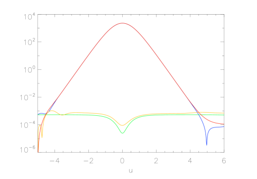
Figure 11: The absolute values of various contributions in (145a) to the energy density for an adiabatic state when $m=H$ are shown for a matching time of $u_{0}=-5$. The blue curve is the total energy density, the red curve is the contribution from the ${\cal N}_{k}$ term, the green curve is the contribution from $\varepsilon_{\rm vac}$, and the orange curve is the contribution from the sum of the ${\cal R}_{k}$ and the ${\cal I}_{k}$ terms. Note the logarithmic scale.

One way to assess the usefulness of the particle description is to analyze its contribution to the stress-energy tensor. This is done in Fig. 11 where the full energy density and that due to the various terms in the energy density (145) are plotted. It is clear from the plot that near $u=0$ the $\varepsilon_{k}^{\cal N}{\cal N}_{k}$ term provides by far the dominant contribution to the stress-energy tensor. At very early times and very late times this is not the case. At early times this is expected since the particle definition is designed to give a vacuum state at the matching time. At late times it is also expected since the energy density of the particles redshifts away.

Figure 12: The product of the fourth power of the scale factor and the energy density for an adiabatic state when $m=H$ is shown. The matching time for the adiabatic state is $u_{0}=-5$.

From the window function (108) in the contracting phase of de Sitter space the energy density for the initial adiabatic vacuum matched by (102) at $u=u_{0}$ should behave like

$$\varepsilon_{{}_{R}}\simeq\frac{1}{2\pi^{2}a^{3}}\sum_{k=K_{\gamma}(u)}^{K_{\gamma}(u_{0})}\,k^{2}\varepsilon_{k}^{\cal N}\,\Delta{\cal N}_{1\,k\gamma}\simeq\frac{1}{8\pi^{2}}\frac{K^{4}_{\gamma}(u_{0})}{a^{4}(u)}\,\frac{1}{e^{8\pi\gamma}-1}\simeq\frac{\gamma^{4}}{8\pi^{2}}\frac{1}{e^{2\pi\gamma}-1}\,\frac{\sinh^{4}u_{0}}{a^{4}(u)}$$ (148)

and therefore grow exponentially with the fourth power of the scale factor as $a(u)$ decreases, consistent with our discussion above of the highest $k$ modes contributing in the window $K(u)<k<K(u_{0})$ in the contracting phase, where their effects on the stress tensor are blueshifted, becoming highly relativistic. This is what accounts for the enormous growth of the particle contribution to the energy density $\varepsilon_{k}^{\cal N}$ in Fig. 11 as it rapidly dominates the quantum $\varepsilon_{k}^{\cal R},\varepsilon_{k}^{\cal I}$ and vacuum terms in (145). This is completely analogous to the secular growth of the current in a constant uniform electric field starting from the adiabatic vacuum plotted in Fig. 4. To check the $a^{-4}$ relativistic dependence predicted by (148) we plot the energy density due to the particles multiplied by $a^{4}(u)$ in Fig. 12. As expected the resulting quantity is approximately constant for a large range of $u$, deviating from this behavior only for initial values of $u$ of order $u_{0}<0$ and again as the particles are redshifted away at $u$ of order $|u_{0}|$.

The estimate (148) also predicts that the maximum value of the energy density at the symmetric point $u=0$ varies with the fourth power of $\sinh u_{0}$. In Fig. 13 the energy density is plotted for two different adiabatic matching times. It is also clear from the plots that the maximum energy density at $u=0$ is substantially larger for the earlier adiabatic matching time, consistent with (148). This is expected since an earlier matching time allows more modes to go through the first particle creation phase and increases the upper limit $K_{\gamma}(u_{0})$ in (148).

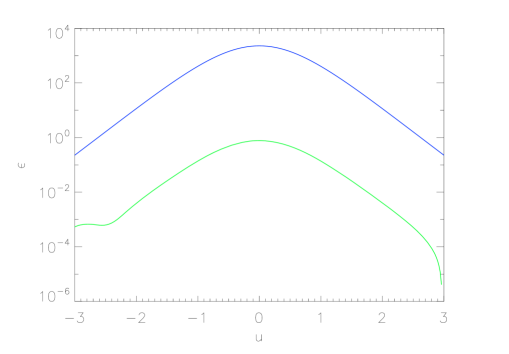
Figure 13: The energy density for an adiabatic state when $m=H$ is shown for an adiabatic matching time of $u_{0}=-3$ (green curve) and a matching time of $u=-5$ (blue curve).

These results show that the adiabatic particle definition is a very useful one, since its contribution to the energy density dominates when the particles become ultrarelativistic, that the energy density of the created particles grows exponentially in the contracting phase of de Sitter space, and most importantly that the maximum of the energy density also grows exponentially with the initial time as $u_{0}\rightarrow-\infty$. This shows conclusively that global or ‘eternal’ de Siter space is unstable to particle creation, as their arbitrarily large energy densities will necessarily lead to a very large backreaction on the classical spacetime when used as a source for the semi-classical Einstein equations, especially as $u_{0}\rightarrow-\infty$.

That the effect grows in the contracting phase of de Sitter, when modes are being blueshifted to the ultrarelativistic regime, and the large $k$ UV part of the mode sum dominates, as opposed to the expanding phase when the particles are redshifted and the low $k$ modes dominate is not surprising. To see this effect properly one needs to start with the adiabatic basis at a finite (early) initial time. We observe here one major difference between the electric field and de Sitter cases in the basic kinematics. The electric field is a vector field and uniformly accelerates all charged particles of a given charge in one direction. Particles (virtual or real) with initially negative kinetic momenta along the direction of the electric field are eventually brought momentarily to rest, and then turn around with continually increasing positive kinetic momentum ever after. It is these modes in the quantum theory that undergo particle creation at the turnaround time, and make the secular contribution to the current as their kinetic momentum and energy grow without bound and the corresponding particles approach the speed of light. Thus this late time contribution is clearly relativistic and UV dominated. There is only one creation event for each wavenumber mode.

On the other hand in the de Sitter case the physical or kinetic momentum is $p=k/a$ which is isotropic, depending only on the magnitude of $\bf k$ and not its direction in the spatially homogeneous states we are considering. There are two creation events for each $k$ mode, one in the contracting phase of de Sitter space, the second in the expanding phase. The first creation event is quite analogous to the electric field case in that once created the particles are blueshifted (exponentially in this case), rapidly becoming ultrarelativistic and making a contribution to the energy density and pressure that grows like $a^{-4}$, typical of ultrarelativistic particles in the contracting phase of de Sitter space. In the expanding phase of de Sitter space the situation is reversed, the created particles are redshifted and make a decreasing contribution to the stress tensor, at least for spatially homogeneous states, so that even a steady rate of particle creation cannot produce an effect in the stress tensor secularly growing in time. Instead the vacuum and other $\cal R$ and $\cal I$ interference terms in (145) remain of the same order as the particle creation term at late times and together their sum approaches the de Sitter invariant CTBD value Attract . There is no exact analog of this second behavior in the electric field case.

IX Adiabatic Switching On of de Sitter Space and the In Vacuum

In the case of the spatially uniform electric field there is an exactly soluble problem in which the electric field is adiabatically switched on and off according to the profile

$$A_{z}(t)=-E\,T\,\tanh\left(t/T\right)\,,\qquad{\bf E}(t)=E\,{\bf\hat{z}}\ {\rm sech}^{2}\left(t/T\right)\;.$$ (149)

By taking the limit $T\rightarrow\infty$ at the end of the calculation, the constant uniform field (49) is recovered Nik ; NarNik ; GavGit . On the other hand if $T$ is finite and $t\rightarrow\pm\infty$ the electric field goes to zero exponentially rapidly, and the particle and anti-particle solutions are the standard Minkowski ones (with $p=k_{z}\pm eET$), so there is no doubt that ${\it in}$ and ${\it out}$ states may be identified with the Minkowski vacuum and the excitations above that state correspond to the usual definition of particles.

No such analytically soluble model for de Sitter space is known. However there is no difficulty in studying the time profile of the scale factor

$$a_{T}(u)=\frac{1}{H}\,\cosh\bigg{[}HT\tanh\left(\frac{u}{HT}\right)\bigg{]}$$ (150)

in the line element (2) and the associated solutions of the scalar field mode equation (16) by numerical methods. With this profile at fixed $T$, in the infinite time limits $u\rightarrow\mp\infty$, $a(u)$ approaches the constant $H^{-1}\cosh(HT)$ so that the spacetime is static and the particle number is uniquely defined by the asymptotic constant positive and negative frequency functions. On the other hand for $HT\rightarrow\infty$ at fixed $u$, $a_{T}(u)$ approaches the de Sitter scale factor $H^{-1}\cosh u$. Thus (150) interpolates between static spacetimes in both the remote past and remote future with a symmetrical de Sitter contracting and expanding phase in between.

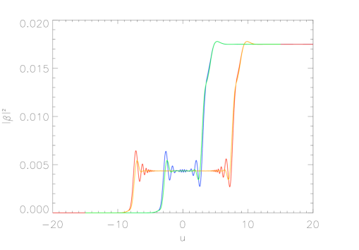
Figure 14: Comparison of $|\beta_{k}(u)|^{2}$ for the in vacuum in exact de Sitter space for matching time $u_{0}=-15$, and that for the smooth adiabatic switching on of de Sitter space according to the time profile (150) for $HT=1000$. Plotted is $|\beta_{k}(u)|^{2}$ for $k=10$, $u_{0}=-15$ (green, exact and blue, $HT=1000$), and $|\beta_{k}(u)|^{2}$ for $k=1000$, $u_{0}=-15$ $HT=1000$ (red, exact and orange, $HT=1000$ ).

In Fig. 14 we show a comparison of the time dependent adiabatic particle number $|\beta_{k}(u)|^{2}$ for the fixed de Sitter and adiabatic switched metric of the form (150), for two representative values of $k$. The similarity of the curves for the two models with the same value of $k$ shows that essentially the same particle production process takes place in the fixed de Sitter space background or with the adiabatic switching on of the background from a static initial metric according to (150), at least for a large range of $k$ when $T$ is large enough. This supports the choice of the in state and positive frequency mode function (30a) in de Sitter space, as that one selected by turning on the de Sitter background adiabatically. Certainly the state produced in this way is very different from the maximally symmetric CTBD state defined by analytic continuation from Euclidean ${\mathbb{S}}^{4}$, in its low momentum modes, as expected by our analysis of adiabatic vacua and particle creation: compare Fig. 10. A detailed study of the state and subsequent evolution produced by (150) and other adiabatic profile functions will be presented in a subsequent publication AndMotSan .

X Summary and Discussion

In this paper we have presented a detailed study of the spontaneous particle production of a massive free field theory in geodesically complete de Sitter space in real time. It is this spontaneous production of particles from the vacuum that is the basis for the instability of global de Sitter space. The formulation of particle creation as an harmonic oscillator with a time dependent frequency, or equivalently, as a one-dimensional stationary state scattering problem, determines the in and out positive energy particle states for massive fields in de Sitter space. This emphasizes the very close analogy with the spontaneous creation of charged particle/anti-particle pairs in a uniform, constant electric field. In each case the background gravitational or electric field configuration is symmetric under time reversal. Hence in each case it is possible to find a time reversal symmetric state in which no net particle creation occurs, and for which the imaginary part of the one-loop effective action and the decay rate vanishes identically. Such a maximally symmetric state allows a ‘self-consistent’ solution of the semi-classical Maxwell or Einstein equations, with vanishing electric current or de Sitter invariant stress-tensor. The artificiality of such a time symmetric state is apparent in the stationary scattering formulation, since it corresponds to choosing a very special coherent superposition of positive and negative frequency scattering solutions globally, which exactly cancels each spontaneous particle creation event by a time reversed particle annihilation event, c.f. Fig. Fig:CTBD. This corresponds to adjusting the state of the quantum field to contain just as many pairs coming in from infinity and with the precisely right phase relations between them, so as to exactly cancel the electric currents or stress-energies of the pairs being spontaneously produced by the electric or de Sitter backgrounds. This is clearly not a true vacuum state in either case.

In situations such as these, the extension of the concepts of ‘particle’ and ‘vacuum’ from flat Minkowski space with no background fields must be reconsidered carefully. The essential generalization of the Feynman prescription of particles propagating forward in time and anti-particles propagating backward in time is to define in and out ‘vacuum’ states corresponding to the choice of pure positive frequency modes (74) at intermediate times which are asymptotic to the exact particle in and out solutions (33) of the oscillator equation (16) in the remote past and remote future. Mathematically this is the condition that the positive frequency particle modes are analytic functions of $m^{2}$ in the upper or lower complex plane which are regular as $t\rightarrow\mp\infty$ respectively, and which corresponds also to the Schwinger-DeWitt method and choice of proper time contour. This should settle the question of whther the effective action in de Sitter space is real or imaginary due to particle creation effects Akhm .

We have provided evidence that the in state is also the state obtained by turning the background fields on and off again according to a finite time $T$ parameter which may be taken to infinity at the end of all calculations. By any of these equivalent methods one obtains the standard Schwinger decay rate (73) for scalar charged particle creation in a constant, uniform electric field. By applying these same two methods to the background gravitational field of de Sitter space, one obtains the vacuum persistence amplitude and decay rate (46). Hence global de Sitter space is unstable to particle creation for the same reason as a constant, uniform electric field is in electrodynamics. This provides a mechanism for the relaxation of vacuum energy into matter or radiation and at least one possible route to the solution of the vacuum energy problem relying only upon known physics Fluc ; NJP .

Although the definition of the adiabatic particle number (81) necessarily comes with some ambiguity in a time dependent background, and depends upon two frequency functions $(W_{k},V_{k})$ in (84) that are not unique, their choice is highly constrained by the requirements of rendering the vacuum zero-point contributions to physical currents, and the energy density and pressure (142) ultraviolet finite. The detailed time profile of the particle number depends upon the particular choice of adiabatic particle number through $(W_{k},V_{k})$, but the qualitative features and the asymptotic values in either the constant electric field or de Sitter cases do not, c.f. Figs. 1 and 8. The rapid change in the adiabatic particle number around ‘creation events’ can be understood from the location of the zeroes of the adiabatic frequency function in the complex time plane, c.f. (87) and Figs. 2-3 in the electric field case and (103) and Figs. 5-9 for de Sitter space. Some adiabatic particle number definition of this kind is certainly necessary to make the transition from QFT to kinetic theory, since the Boltzmann equation assumes that particle numbers and densities can be defined.

The usefulness of the particle concept is seen in the evaluation of expectation values of currents and stress tensors, and particularly in their secular terms, which are most important for backreaction. The ‘window function’ (91) of pair creation in the electric field background accounts very well for the linear secular growth in time of the current of the produced pairs in Fig. 4 QVlas . In the de Sitter case the corresponding window function (108) accounts very well for the exponential growth of the energy density and pressure of the created particles in the contracting phase, c.f. Eq. (148) and Fig. 11. The linear growth in time in the first case and exponential $a^{-4}$ growth in time in the contracting de Sitter case, Fig. 12 are just what should be expected as the created particles are accelerated and rapidly become ultrarelativistic. Because of this secular growth backreaction effects on the background electric field must be taken into account through the semi-classical Maxwell equations. Likewise for the de Sitter geometry for early enough matching times $u_{0}$, c.f. 148), backreaction effects similarly must be taken into account through the semi-classical Einstein equations.

This detailed study of particle creation removes a possible objection to the use of the strictly asymptotic in and out states in PartCreatdS to calculate the decay rate of de Sitter space, namely that these states are not Hadamard UV allowed states as defined e.g. in ShortDistDecohere . Instead they are members of the one parameter family of ‘$\alpha$ vacua’ invariant under the $SO(4,1)$ subgroup of the de Sitter group continuously connected to the identity PartCreatdS ; Allen , although not the discrete ${\mathbb{Z}}_{2}$ inversion symmetry (154). The difficulty is removed by the recognition that the large $|u|$ time and large $k$ limits do not commute. If one starts with UV allowed states such as the adiabatic initial state (102) at a finite initial time, and evolves forward for a finite time, only a finite number of modes experience particle creation events, according to the appropriate window function. The non-Hadamard $\alpha$ vacua are produced only in the improper limit of $|u|\rightarrow\infty$ in eternal de Sitter space, never in any finite time starting with UV finite initial data. Although the result for the decay rate (46) with an appropriate physical cutoff is the same, only a detailed analysis of the $k$ and time dependence allows a description free of any spurious UV problems and focuses attention on the resulting necessary breaking of de Sitter invariance instead Fluc ; deSMM .

In the electric field case it is generally accepted that particle creation will lead to eventual ‘shorting’ of the electric field, although to date this process has only been studied in a large $N$ semiclassical approximation KESCM , which is not adequate to show the true long time behavior of the system even in QED. This depends upon self-interactions, and the long time behavior of correlation functions that are not accessible to the standard weak coupling approximations. Such processes involving multiple interactions in a medium, possibly very far from equilibrium, are generally described in many-body physics in the kinetic Boltzmann equation approximation, where all time reversal invariance properties of the underlying QFT are lost, and irreversible behavior is expected. What is perhaps less widely appreciated is that this breaking of time reversal invariance has its roots in the definition of the vacuum itself and the distinction between particles and anti-particles in QFT by the $m^{2}-i0^{+}$ prescription for the Feynman propagator and Schwinger-DeWitt proper time method. When interactions are turned on, the bare mass becomes a dressed self-energy function $\Sigma-i{\Gamma}/2$ and the pole moves away from the real axis. The imaginary part is now finite and gives the quasi-particle lifetime in the medium. Causality fixes the sign of this imaginary part, and that same causal prescription is already present in the free propagator in the limit $\Gamma\rightarrow 0^{+}$ that the interactions are turned off. It is this causal boundary condition anticipating the inclusion of interactions, rather than the interactions themselves, which breaks time reversal symmetry.

Spontaneous particle creation vs. the exact annihilation of particles in the CTBD state, ​c.f. Fig. 10 raises another interesting point about the origins of time irreversibility, entropy and the second law in QFT. That particle creation is in some sense an irreversible process in which entropy increases HuKanPav can be made precise by means of the quantum density matrix expressed in the adiabatic particle basis. Since adiabatic particle number is by construction an adiabatic invariant of the evolution, the diagonal elements of the density matrix are slowly varying in this basis. In contrast, the off-diagonal elements are rapidly varying functions both of time and of momentum at a fixed time. Then it is reasonable to average over those rapidly varying phases and construct the reduced density matrix which shows general (though not strictly monotonic) increase in time as particles are created CKHM , much as Figs. 3, 6 and 7 for the particle number itself do. This is equivalent to the approximation of neglecting the oscillatory term(s) in the current (93) or stress-tensor (145) expectation values, which as we have seen is a very good approximation over long times when the secular effects of particle creation dominate. Clearly no such interpretation is possible for the time symmetric CTBD state in which phase correlations are exactly preserved, and particle annihilations represent a decrease in the effective entropy. One would expect such processes to be statistically disfavored.

The fact that particles can achieve arbitrarily high energies for persistent constant field backgrounds producing a secular effect in both the electric field and de Sitter cases underscores the interesting interplay of UV and IR aspects. Since anomalies perform exactly this function of connecting the UV to the IR, they can play an important role DSAnom ; Zak , a connection we explore in detail in AndMotDSVacua . In de Sitter space with ${\mathbb{S}}^{3}$ spatial sections the blueshifting toward ultrahigh energies is clear in the contracting phase. In the expanding phase of de Sitter space the created particles defined in the ${\mathbb{S}}^{3}$ sections are redshifted and do not produce any growing secular effect in spatially homogeneous states. In fact, one can prove that the energy density and pressure always tend to the de Sitter invariant Bunch-Davies value for fields with positive effective masses, $m^{2}+\xi R>0$, produced in any UV allowed $O(4)$ invariant state Attract . It is this redshifting and damping effect of the expansion upon perturbations in FRW metrics, which because of inflation almost all attention has been focused, and consideration only of spatially homogenous states that leads to the impression that de Sitter space is stable.

This is clearly incorrect for global (’eternal’) de Sitter space which has both a contracting and an expanding phase. In fact, apart from initial conditions or boundary conditions, de Sitter space is a homogeneous manifold in which all points are equivalent, so the very notions of expansion or contraction have no meaning unless a preferred set of de Sitter breaking set of time slicings is chosen. With the ${\mathbb{S}}^{3}$ time slicing chosen to cover all of de Sitter space, for early matching times (as discussed above), the exponentially growing energy density and pressure of the created particles will necessarily produce an enormous backreaction on the geometry if taken into account even semi-classically, and even without self-interactions. Hence one may never arrive at the expanding or inflationary phase of de Sitter space at all. This emphasizes the importance of and sensitivity to the initial conditions of inflation Vil .

Moreover although the description of adiabatic vacua and particle definition given is dependent upon spatial homogeneity and isotropy in the ${\mathbb{S}}^{3}$ time slicings, the tendency to create particles and the possibility for these particles to be kinematically blueshifted and produce large backreaction effects in de Sitter space, is not dependent upon coordinate choices. We have shown in Sec. VII that even in the Poincaré coordinates with flat spatial sections which cover only the expanding half of de Sitter space, particle production also takes place. If only the expanding half of de Sitter space is considered, then the particles are redshifted, so that their energy density does not grow, if the initial state is given and if the particle modes are defined with respect the usual FRW spatially flat sections. Once it is granted that global de Sitter space with its exact $O(4,1)$ symmetry is unstable to particle creation, then there is no reason to restrict one’s attention a priori even to spatially homogeneous or isotropic sections. Fluctuations in the mean stress tensor $\langle T_{ab}(x)T_{cd}(x^{\prime})\rangle$ due to particle creation are surely spatially inhomogeneous. A previous study of linear response has indicated the importance of spatially inhomgeneous perturbations on the de Sitter horizon, in the static coordinates of de Sitter space DSAnom .

Here again the electric field example may be helpful. One can describe a constant, uniform electric field in either a time dependent or time independent but spatially dependent gauge. Both are equally good for describing the idealized situation without boundaries in either space or time. However, what actually happens depends sensitively on boundary or initial conditions. Just as one can consider relaxing the constancy in time of the background to study the dependence upon vacuum initial conditions, adiabatically switching it on and then off, one could also consider the arguably more physical situation of relaxing strict spatial homogeneity, allowing the electric field to be established by some charge distribution at a large but finite distance away from the local region of interest. Sensitivity of the vacuum to initial conditions will likely then be accompanied by sensitivity to the spatial boundary conditions, and the final evolution may be quite different globally. The distance scale over which the particle creation takes place is of order $2mc^{2}/eE$ in an electric field background, so that is the scale at which one might expect spatial inhomogeneities to develop in a random particle creation process. The natural scale for such inhomogenities to develop in de Sitter space is the horizon scale $H^{-1}$. Therefore one should allow for perturbations on the horizon scale which can be sensitive to the blueshifting kinematics in a way that perturbations based on the spatially homogeneous ${\mathbb{S}}^{3}$ or flat Poincaré sections are not. We address spatially inhomogeneous perturbations of the CTBD state in an accompanying paper AndMotDSVacua , depending upon the direction of $\bf k$ as well as its magnitude, and show that these effects may be even more significant that the average particle creation rate in spatially homogeneous states studied in this paper.

Acknowledgements

P. R. A. would like to thank Dillon Sanders for help with the early stages of this project. This work was supported in part by the National Science Foundation under Grant Nos. PHY-0856050 and PHY-1308325. The numerical computations herein were performed on the WFU DEAC cluster; we thank WFU’s Provost Office and Information Systems Department for their generous support.

Appendix A Geometry and Coordinates of de Sitter Space

The de Sitter manifold is most conveniently defined as the single sheeted hyperboloid

$$\eta_{AB}X^{A}X^{B}=-(X^{0})^{2}+\sum_{i=1}^{3}X^{i}X^{i}+(X^{4})^{2}=\frac{1}{H^{2}}$$ (151)

embedded in five dimensional flat Minkowski spacetime,

$$ds^{2}=\eta_{AB}\,dX^{A}\,dX^{B}=-(dX^{0})^{2}+(dX^{1})^{2}+(dX^{2})^{2}+(dX^{3})^{2}+(dX^{4})^{2}\,.$$ (152)

This manifold has the isometry group $O(4,1)$ with the maximal number of continuous symmetry generators ($10$) for any solution of the vacuum Einstein field equations,

$$R^{a}_{\ b}-\frac{R}{2}\,\delta^{a}_{\ b}+\Lambda\,\delta^{a}_{\ b}=0$$ (153)

in four dimensions. It also has the discrete inversion symmetry

$$X^{A}\rightarrow-X^{A}$$ (154)

which is not continuously connected to the identity, making the isometry group of the full de Sitter manifold $O(4,1)={\mathbb{Z}}_{2}\otimes SO(4,1)$. The Riemann tensor, Ricci tensor, and scalar curvature are

$$R^{ab}_{\ \ cd} = H^{2}\left(\delta^{a}_{\ c}\,\delta^{b}_{\ d}-\delta^{a}_{\ d}\,\delta^{b}_{\ c}\right)$$ (155a)

$$R^{a}_{\ b} = 3H^{2}\,\delta^{a}_{\ b}$$ (155b)

$$R = 12H^{2}$$ (155c)

with the Hubble constant $H$ related to $\Lambda$ by

$$H=\sqrt{\frac{\Lambda}{3}}\,.$$ (156)

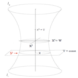
Figure 15: The de Sitter manifold represented as a single sheeted hyperboloid of revolution about the $X^{0}$ axis, embedded in five dimensional flat spacetime $(X^{0},X^{a}),\,a=1,\dots 4$, in which the $X^{1}$, $X^{2}$ coordinates are suppressed. The hypersurfaces at constant $X^{0}=H^{-1}\sinh u$ are three-spheres, $\mathbb{S}^{3}$. The $\mathbb{S}^{3}$ at $X^{0}=\pm\infty$ are denoted by $I_{\pm}$.

The globally complete hyperbolic coordinates $(u,\chi,\theta,\phi)$ of de Sitter space are defined by

$$X^{0} = \frac{1}{H}\,\sinh u\,,$$ (157a)

$$X^{i} = \frac{1}{H}\,\cosh u\,\sin\chi\,\hat{n}^{i}\,,\qquad i=1,2,3\,.$$ (157b)

$$X^{4} = \frac{1}{H}\,\cosh u\,\cos\chi\,$$ (157c)

where $\hat{n}=(\sin\theta\,\cos\phi\,,\sin\theta\,\sin\phi\,,\cos\theta)$ is the unit vector on $\mathbb{S}^{2}$. In these coordinates the de Sitter line element takes the form

$$ds^{2}=\frac{1}{H^{2}}\big{(}-du^{2}+\cosh^{2}u\,d\Sigma^{2}\big{)}$$ (158)

where

$$d\Sigma^{2}\equiv d\hat{N}\cdot d\hat{N}=d\chi^{2}+\sin^{2}\chi\,(d\theta^{2}+\sin^{2}\theta\,d\phi^{2})$$ (159)

is the standard round metric on $\mathbb{S}^{3}$. Hence in the coordinates of (157) which cover the entire de Sitter manifold the de Sitter line element (158) is a hyperboloid of revolution whose constant $u$ sections are three-spheres, c.f. Fig. 15. In (159) and the following we make use of the shorthand notation,

$$\hat{N}=(\sin\chi\ \hat{n},\,\cos\chi)$$ (160)

for the unit four-vector of $\mathbb{S}^{3}$ in the $(X^{i},X^{4})$ coordinates of the flat space embedding.

In cosmology it is more common to use instead the Friedmann-Lemaître-Robertson-Walker (FLRW) line element with flat $\mathbb{R}^{3}$ spatial sections, viz.

$$ds^{2}=-d\tau^{2}+e^{2H\tau}\,d{\bf x}^{2}=-d\tau^{2}+e^{2H\tau}\,(d\varrho^{2}+\varrho^{2}d\Omega^{2})$$ (161)

with $\varrho\equiv|{\bf x}|$. De Sitter space (151)-(152) can be brought into the flat FLRW form (161) by setting

$$X^{0} = \frac{1}{H}\sinh(H\tau)+\frac{H\varrho^{2}}{2}\,e^{H\tau}$$ (162a)

$$X^{i} = e^{H\tau}\,\varrho\,\hat{n}^{i}\,,\qquad i=1,2,3$$ (162b)

$$X^{4} = \frac{1}{H}\cosh(H\tau)-\frac{H\varrho^{2}}{2}\,e^{H\tau}\,.$$ (162c)

From (162) $T+W>0$ in these coordinates for all $\tau\in(-\infty,\infty)$, with the hypersurfaces of constant FLRW time $\tau$ slicing the hyperboloid in Fig. 15 at a $45^{\circ}$ angle. The null surface at $T+W=0$ is approached in the limit $\tau\rightarrow-\infty$.

Hence the flat FLRW coordinates (161) break the time inversion symmetry of global de Sitter space and cover only one half of the full de Sitter hyperboloid in which the spatial sections are always expanding as $\tau$ increases. The other half of the full de Sitter hyperboloid with $T+W<0$ is obtained if $H\tau$ is replaced by $-H\tau^{\prime}+i\pi$, so that $\exp(H\tau)$ is replaced by $-\exp(-H\tau^{\prime})$, and the line element (161) now takes the form

$$ds^{2}=-d\tau^{\prime\,2}+e^{-2H\tau^{\prime}}\,d{\bf x}^{2}$$ (163)

with the spatial sections are always contracting as $\tau^{\prime}$ increases. The null surface $T+W=0$ is approached in the limit $\tau^{\prime}\rightarrow+\infty$.

References

- (1)
-
(2)
- (3) W. Pauli (unpublished); C. P. Enz and A. Thellung, Helv. Phys. Acta 33 839 (1960).
- (4) See e. g. A. R. Liddle and D. H. Lyth, Cosmological Inflation and Large-Scale Structure, Cambridge Univ. Press, Cambridge (2000); or V. Mukhanov, Physical Foundations of Cosmology, Cambridge Univ. Press, Cambridge (2005).
- (5) A. G. Riess et. al., Astron. J. 116, 1009 (1998); S. Perlmutter et. al., Astrophys. J. 517, 565 (1999); J. L. Tonry et. al., Astrophys. J. 594, 1 (2003).
- (6) L. Parker, Phys. Rev. Lett. 21, 562 (1968); Phys. Rev. 183, 1057 (1969); Phys. Rev. D 3, 346 (1971), Erratum ibid. 2546 (1971); Phys. Rev. Lett. 28, 705 (172), Erratum ibid. 1497 (1972).
- (7) Ya.B. Zel’dovich, Pis. Zh. Eksp. Teor. Fiz. 12, 443 (1970) [JETP Lett. 12, 307 (1970)].
- (8) L. Parker and S. A. Fulling, Phys. Rev. D 9, 341 (1974); S. A. Fulling and L. Parker, Ann. Phys. 87, 176 (1974); S. A. Fulling, L. Parker, and B. L. Hu, Phys. Rev. D 10, 3905 (1974).
- (9) N. D. Birrell, Proc. R. Soc. Lon. B 361, 513 (1978); T. S. Bunch, J. Phys. A: Math. Gen. 13, 1297 (1980).
- (10) N. D. Birrell and P. C. W. Davies, Quantum Fields in Curved Space Cambridge Univ. Press, Cambridge (1982).
- (11) E. Mottola, Phys. Rev. D 31, 754 (1985).
- (12) E. Mottola, Phys. Rev. D 33, 2136 (1986); Physical Origins of Time Asymmetry, J. J. Halliwell et al. eds., pp. 504-515, Cambridge, Cambridge Univ. Press (1993).
- (13) I. Antoniadis, P. O. Mazur and E. Mottola, New J. Phys. 9, 11 (2007).
- (14) A. M. Polyakov, Nucl. Phys. B 797, 199 (2008); ibid. 834, 316 (2010); e-print arXiv:1209.4135; D. Krotov and A. M. Polyakov, Nucl. Phys. B 849, 410 (2011).
- (15) E. T. Akhmedov and P.V. Buividovich, Phys. Rev. D 78, 104005 (2008).
- (16) O. Nachtmann, Commun. Math. Phys. 6, 1 (1967).
- (17) N. A. Chernikov and E. A. Tagirov, Ann. Inst. H. Poincaré Phys. Theor. A9, 109 (1968); E. A. Tagirov, Ann. Phys. 76, 561 (1973).
- (18) T. S. Bunch and P. C. W. Davies, Proc. R. Soc. A 360, 117 (1978).
- (19) G. W. Gibbons and S. W. Hawking, Phys. Rev. D 15, 2738 (1977); A. S. Lapedes, J. Math. Phys. 19, 2289 (1978).
- (20) L. H. Ford, Phys. Rev. D 31, 710 (1985).
- (21) I. Antoniadis and E. Mottola, preprint CERN-TH-4605/86 (1986); Jour. Math. Phys. 32, 1037 (1991).
- (22) N. C. Tsamis and R. P. Woodard, Nuc. Phys. B 474, 235 (1996); Ann. Phys. 253, 1 (1997); 267,145 (1998).
- (23) J. Schwinger, Phys. Rev. 82, 664 (1951).
- (24) B. S. DeWitt Dynamical Theory of Groups and Fields, Gordon and Breach, New York (1965); Phys. Rep. 19, 295 (1975).
- (25) H. Rumpf, Phys. Lett. B 6, 272 (1976); Nuovo Cim. B35, 321 (1976); H. Rumpf and H. K. Urbantke, Ann. Phys. 114, 332 (1978).
- (26) N. B. Narozhnyi, Zh. Eksp. Teor. Fiz. 54, 676 (1968) [Sov. Phys. JETP 27, 360 (1968)].
- (27) A. I. Nikishov, Zh. Eksp. Teor. Fiz. 57, 1210 (1970) [Sov. Phys. JETP 30, 660 (1970)].
- (28) N. B. Narozhnyi and A. I. Nikishov, Yad. Fiz. 11, 1072 (1970) [Sov. J. Nuc. Phys. 11, 596 (1970)].
- (29) E. S. Fradkin, D. M. Gitman, and Sh. M. Shvartsman, Quantum Electrodynamics with Unstable Vacuum, Springer-Verlag, Berlin (1991).
- (30) F. Cooper, E. Mottola, B. Rogers, and P. Anderson, “Pair Production From an External Electric Field”, in the Proceedings of the Santa Fe Workshop on Intermittency in High Energy Collisions, edited by F. Cooper, R. Hwa and I. Sarcavic (World Scientific, 1991) p. 399; Y. Kluger, J. M. Eisenberg, B. Svetitsky, F. Cooper, and E. Mottola, Phys. Rev. Lett. 67, 2427 (1991); Phys. Rev. D 45, 4659 (1992); F. Cooper, J. M. Eisenberg, Y. Kluger, E. Mottola, and B. Svetitsky, Phys. Rev. D 48, 190 (1993).
- (31) S. O. Gavrilov and D. M. Gitman, Phys. Rev. D 53, 7162 (1996).
- (32) Y. Kluger, E. Mottola, and J. M. Eisenberg, Phys. Rev. D 58, 125015 (1998).
- (33) P. R. Anderson and E. Mottola, LA-UR-13-26990, submitted to Phys. Rev. D.
- (34) S. Habib, C. Molina-París and E. Mottola, Phys. Rev. D 61, 024010 (1999).
- (35) P. R. Anderson, W. Eaker, S. Habib, C. Molina-París, and E. Mottola, Phys. Rev. D 62, 124019 (2000).
- (36) R. P. Feynman, Phys. Rev., 76, 749 (1949).
- (37) R. P. Feynman, Rev. Mod. Phys., 20, 367 (1948); R. P. Feynman and A. R. Hibbs, Quantum Mechanics and Path Integrals, McGraw-Hill, New York (1965).
- (38) Higher Transcendental Functions, Vols. I and II, Bateman Manuscript Project, A. Erdélyi, ed. McGraw-Hill, New York (1953).
- (39) M. Gutzwiller, Helv. Phys. Acta 29, 213 (1956).
- (40) H. Rumpf, Phys. Rev. D 24, 275 (1981).
- (41) A. R. Bell and J. G. Kirk, Phys. Rev. Lett. 101, 200403 (2008); D. B. Blaschke, A. V. Prozorkevich, G. Ropke, C. D. Roberts, S. M. Schmidt, D. S. Shkirmanov, and S. A. Smolyansky, Eur. Phys. J. D 55, 341 (2009); G. V. Dunne, H. Gies, and R. Schützhold, Phys. Rev. D 80, 111301 (2009); G. V. Dunne, Int. J. Mod. Phys. A 25, 2373 (2010).
- (42) B. Allen, Phys. Rev. D 32, 3136 (1985).
- (43) V. L. Pokrovskii and I. M. Khalatnikov, Zh. Eksp. Teor. Fiz. 40, 1713 (1961) [Sov. Phys. JETP 13, 1207 (1961)].
- (44) P. R. Anderson, E. Mottola, and D. H. Sanders, in preparation.
- (45) J. Schwinger, Phys. Rev. 125, 397 (1962); 128, 2425 (1962).
- (46) S. Coleman, Phys. Rev. D 11, 2088 (1975); J. Fröhlich and E. Seiler, Helv. Phys. Acta 49, 889 (1976).
- (47) K. Johnson, Phys. Lett. 5, 253 (1963).
- (48) P. R. Anderson and L. Parker, Phys. Rev. D 36, 2963 (1987).
- (49) P. R. Anderson and W. Eaker, Phys. Rev. D61, 024003 (1999).
- (50) P. R. Anderson, C. Molina-París, and E. Mottola, Phys. Rev. D 72, 043515 (2005).
- (51) E. T. Akhmedov, Mod. Phys. Lett. A25, 2815 (2010).
- (52) P. O. Mazur and E. Mottola, Nucl. Phys. B 278, 694 (1986).
- (53) B. L. Hu and D. Pavon, Phys. Lett. B 180, 329 (1986); B. L. Hu and H. E. Kandrup, Phys. Rev. D 35, 1776 (1987).
- (54) S. Habib, Y. Kluger, E. Mottola, and J. P. Paz, Phys. Rev. Lett. 76, 4660 (1996); F. Cooper, S. Habib, Y. Kluger, and E. Mottola, Phys. Rev. D 55, 6471 (1997).
- (55) P. R. Anderson, C. Molina-París, and E. Mottola, Phys. Rev. D 80, 084005 (2009).
- (56) E. Mottola, Acta Physica Polonica B 41, 2031 (2010).
- (57) A. Vilenkin, Phys. Rev. D 46, 2355 (1992).