The Cosmic Evolution of Fermi BL Lacertae Objects

Abstract

Fermi has provided the largest sample of $\gamma$-ray selected blazars to date. In this work we use a uniformly selected set of 211 BL Lacertae (BL Lac) objects detected by Fermi during its first year of operation. We have obtained redshift constraints for 206 out of the 211 BL Lacs in our sample making it the largest and most complete sample of BL Lacs available in the literature. We use this sample to determine the luminosity function of BL Lacs and its evolution with cosmic time. We find that for most BL Lac classes, the evolution is positive with a space density peaking at modest redshift (z$\approx$1.2). The low-luminosity, high-synchrotron peaked (HSP) BL Lacs are an exception, showing strong negative evolution, with number density increasing for z$\lesssim$0.5. Since this rise corresponds to a drop-off in the density of flat-spectrum radio quasars (FSRQs), a possible interpretation is that these HSPs represent an accretion-starved end-state of an earlier merger-driven gas-rich phase. We additionally find that the known BL Lac correlation between luminosity and photon spectral index persists after correction for the substantial observational selection effects with implications for the so called ‘blazar sequence’. Finally, estimating the beaming corrections to the luminosity function, we find that BL Lacs have an average Lorentz factor of $\gamma=6.1^{+1.1}_{-0.8}$, and that most are seen within 10^∘ of the jet axis.

1 Introduction

BL Lacertae (BL Lac) objects are a sub-population of blazars, an extreme class of active galactic nuclei (AGN), displaying highly variable emission likely due to a relativistic jet pointing close to our line of sight (e.g. Blandford & Rees, 1978). They are distinguished from their siblings, the flat-spectrum radio quasars (FSRQs) by an optical spectrum lacking any emission lines with equivalent width $>$5 $\AA$ (e.g. Urry & Padovani, 1995; Marcha et al., 1996). The optical spectra of BL Lac objects are power-law dominated indicating either especially strong non-thermal continuum (jet aligned very close to our line of sight) or unusually weak thermal disk/broad line emission (plausibly attributed to low accretion activity; Giommi et al., 2012).

The synchrotron component of BL Lacs shows a range of peak frequencies from $\nu\approx$10¹³ Hz up to $\nu\approx$10¹⁷ Hz (e.g. Ackermann et al., 2011). At the high end, these synchrotron peaks imply that BL Lacs are able to accelerate electrons beyond 100 TeV (e.g. Costamante et al., 2001; Tavecchio et al., 2011), making BL Lacs among the most powerful accelerators in the Universe.

The lack of strong emission lines hampers traditional optical spectroscopic measurements of the redshifts of most BL Lac objects. Indeed, roughly 55 % of the 395 BL Lac objects detected in the second Fermi AGN catalog (2LAC, Ackermann et al., 2011) lacked a spectroscopic redshift. This limitation is also serious at lower frequencies (Padovani et al., 2007) and the large redshift incompleteness of most BL Lac samples has hampered so far the determination of a reliable luminosity function. In turn this handicaps studies of the growth and evolution of BL Lac objects in the Universe and the relationship between BL Lacs and the FSRQ class.

While it is clear that FSRQs evolve positively at all frequencies (i.e. there were more blazars in the past, Dunlop & Peacock, 1990) up to a redshift cut-off which depends on luminosity (e.g. Padovani et al., 2007; Wall, 2008; Ajello et al., 2009, 2012), the evolution of BL Lacs remains a matter of debate. Indeed, various studies have found that BL Lac objects evolved negatively (e.g. Rector et al., 2000; Beckmann et al., 2003), positively (e.g. Marcha & Caccianiga, 2013) or not at all (Caccianiga et al., 2002; Padovani et al., 2007). These discrepancies might be due to small samples, biases in the set of BL Lacs and substantial redshift incompleteness in these works.

At gamma-ray energies the need for a reliable Luminosity Function (LF) is particularly acute. Indeed, the present lack of a secure LF makes it impossible to estimate the contribution of faint (below detection threshold) BL Lacs to the isotropic gamma-ray background (IGRB, Abdo et al., 2010b). At GeV-TeV energies BL Lacs are characterized by a harder spectrum than FSRQs and are found to outnumber (by a factor $>$3) the latter particularly above 10 GeV (Abdo et al., 2010c). Thus at high energies these sources may well dominate the cosmic gamma-ray background.

Thanks to the excellent sensitivity, the Large Area Telescope (LAT) on board Fermi has detected $\sim$395 BL Lac objects in the first 2 years of operations (Ackermann et al., 2011). To study this sample many different techniques have been employed to obtain redshift estimates or constraints for these blazars (see Rau et al., 2012; Shaw et al., 2013b, a), yielding the rather surprising detection of several BL Lacs up to redshift z$\approx$2. These high–z objects often show a very hard (photon index of $\sim$2) GeV spectrum making them the most luminous BL Lacs of the high-synchrotron peaked (HSP) kind ever detected. How these objects fit within the scheme of the blazar population and blazar sequence is still highly debated (Padovani et al., 2012; Ghisellini et al., 2012).

In this work we study the cosmological properties of BL Lacs focusing on a complete set of 211 BL Lacs detected by Fermi-LAT during the first year of operation (Abdo et al., 2010d). Using the full range of techniques (see Rau et al., 2012; Shaw et al., 2013b), we have obtained spectroscopic redshifts or limits for the great majority ($\sim$98 %) of the sources. This has let us derive the first detailed models for the luminosity function and evolution of BL Lacs at GeV energies. The large sample size and unusually high redshift completeness allow new inferences about the nature of the BL Lac population, as a whole. This paper is organized as follows: $\S$ 2 and $\S$ 3 present the properties of the sample, discuss the available redshift constraints and describe the method used to derive the luminosity function. The results are presented and discussed in $\S$ 4, 5, and 6. Throughout this paper, a standard concordance cosmology was assumed (H₀=71 km s^-1 Mpc^-1, $\Omega_{M}$=1-$\Omega_{\Lambda}$=0.27).

2 The Sample

The First Fermi LAT Catalog (1FGL, Abdo et al., 2010a) presented more than 1400 sources detected by Fermi-LAT during its first year of operation. The first LAT AGN catalog (1LAC, Abdo et al., 2010d) associates $\sim$700 of the high-latitude 1FGL sources ($|b|\geq 10^{\circ}$) with AGN of various types, most of which are blazars. The sample used for this analysis consists of sources detected by the pipeline developed by Abdo et al. (2010c) with a test statistic (TS) greater (or equal) than 50 and with $|b|\geq$15^∘. For these sample cuts we have produced a set of Monte Carlo simulations that can be used to determine and correct for the selection effects. This sample contains 486 objects, 211 of which are classified as BL Lacs in 1LAC. The composition of this sample is reported in Table 1. The source classifications reported in Table 1 are originally drawn from the 1LAC and 2LAC catalogs (Abdo et al., 2010d), and have been complemented with newer observations reported in Shaw et al. (2012) and Shaw et al. (2013b).

The 211 BL Lacs detected by Fermi with TS$\geq 50$, $|b|\geq 15^{\circ}$, constitute the sample that will be used in this analysis. All these objects are reported together with their properties in the Table reported in the Appendix ($\S$ A.1). We note that fluxes and photon indices reported there are those measured with the pipeline developed by Abdo et al. (2010c) and thus, while compatible with the values reported in the 1FGL catalog (Abdo et al., 2010a), they are not exactly the same. These values are meant to be used with the results of the Monte Carlo simulations to correctly account for selection effects (see $\S$ 4 and $\S$ 5 in Abdo et al., 2010c).

Of the 38 sources remaining unclassified in 1FGL, three objects now have pulsar identifications, two sources have been dropped as spurious composites and 10 are flagged as pulsar candidates based on their variability and spectral properties (Ackermann et al., 2012). This leaves 23 objects which might be blazars yet to be identified. Recent radio observations (Petrov et al., 2013) find compact source counterparts for 11 of these, so it is likely that these 11 represent missing BL Lacs. Moreover, cross-correlating the list of 23 objects with the WISE sources whose colors are typical of blazars (Massaro et al., 2012; D’Abrusco et al., 2012) we found an additional 8 blazar candidates. Thus a total of 19 sources display properties of blazars on the basis of their IR colors or radio properties. Conservatively we assume that all these sources might be BL Lacs, and that the incompleteness (due to missing identification) in our BL Lac sample is 19/211=9 %. The total incompleteness (due to missing redshifts and identifications) is thus $\sim$11 %. As it will be shown later this incompleteness does not constitute a problem for the analysis.

Table 1: Composition of the $|b|\geq$15^∘, TS$\geq$50, sample used in this analysis.

Class	# objects
Total	486
BL Lacs	211
FSRQs	186
Pulsars	31
Dropped by 2FGL	2
Other	33
Unassociated sources	23

3 Analysis

3.1 Method

In order to derive the LF of BL Lacs we rely on the maximum likelihood (ML) method first introduced by Marshall et al. (1983) and used recently for the study of blazars detected by Swift (Ajello et al., 2009) and FSRQs detected by Fermi (Ajello et al., 2012). The aim of this analysis is to determine the space density of BL Lacs as a function of rest-frame 0.1–100 GeV luminosity (L_γ), redshift (z) and photon index ($\Gamma$), by fitting to the functional form:

$$\frac{\partial^{3}N}{\partial L_{\gamma}\partial z\partial\Gamma}=\frac{\partial^{3}N}{\partial L_{\gamma}\partial V\partial\Gamma}\times\frac{dV}{dz}=\Phi(L_{\gamma},V(z),\Gamma)\times\frac{dV}{dz}$$ (1)

where $\Phi(L_{\gamma},V(z),\Gamma)$ is the luminosity function, and $dV/dz$ is the co-moving volume element per unit redshift and unit solid angle (see e.g. Hogg, 1999).

The best-fit LF is found by comparing, through a maximum-likelihood estimator, the number of expected objects (for a given model LF) to the observed number while accounting for selection effects in the detection of gamma-ray sources. In this method, the space of luminosity, redshift, and photon index is divided into small intervals of size $dL_{\gamma}dz\,d\Gamma$. In each element, the expected number of blazars with luminosity $L_{\gamma}$, redshift $z$ and photon index $\Gamma$ is:

$$\lambda(L_{\gamma},z,\Gamma)dL_{\gamma}dzd\Gamma=\Phi(L_{\gamma},V(z),\Gamma)\cdot\Omega(L_{\gamma},z,\Gamma)\ \frac{dV}{dz}\ dL_{\gamma}dzd\Gamma$$ (2)

where $\Omega(L_{\gamma},z,\Gamma)$ is the sky coverage and represents the probability of detecting in this survey a blazar with luminosity $L_{\gamma}$, redshift $z$ and photon index $\Gamma$. This probability was derived for the sample used here by Abdo et al. (2010c) and the reader is referred to that paper for more details. With sufficiently fine sampling of the $L_{\gamma}-z-\Gamma$ space the infinitesimal element will either contain 0 or 1 BL Lac. In this regime one has a likelihood function based on joint Poisson probabilities:

$$L=\prod_{i}\lambda(L_{\gamma,i},z_{i},\Gamma_{i})dL_{\gamma}dzd\Gamma e^{-\lambda(L_{\gamma,i},z_{i},\Gamma_{i})dL_{\gamma}dzd\Gamma}\times\prod_{j}e^{-\lambda(L_{\gamma,j},z_{j},\Gamma_{j})dL_{\Gamma}dzd\Gamma}$$ (3)

This is the combined probability of detecting one blazar in each bin of $(L_{\gamma,i},z_{i},\Gamma_{i})$ populated by one observed Fermi BL Lac and zero BL Lacs for all other $(L_{\gamma,j},z_{j},\Gamma_{j})$. Transforming to the standard expression $S=-2\ln\ L$ and dropping terms which are not model dependent, we obtain:

$$S=-2\sum_{i}{\rm\ln}\frac{\partial^{3}N}{\partial L_{\gamma}\partial z\partial\Gamma}+2\int^{\Gamma_{max}}_{\Gamma_{min}}\int^{L_{\gamma,max}}_{L_{\gamma,min}}\int^{z_{max}}_{z_{min}}\lambda(L_{\gamma},\Gamma,z)dL_{\gamma}dzd\Gamma$$ (4)

The limits of integration of Eq. 4 and subsequent equations, unless otherwise stated, are: $L_{\gamma,min}=7\times 10^{43}$ erg s^-1, $L_{\gamma,max}$=10⁵² erg s^-1, $z_{min}=$0.03, $z_{max}$=6, $\Gamma_{min}=$1.45 and $\Gamma_{max}=$2.80. The results of this analysis are independent of the choice of the maximum redshift and luminosity. All other limits correspond to those spanned by the set of sources analyzed here. The best-fit parameters are determined by minimizing $S$ and the associated 1 $\sigma$ errors are computed via bootstrap analysis (see later). While computationally intensive, Eq. 4 has the advantage that each source has its appropriate individual detection efficiency and k-correction treated independently.

To test whether the best-fit LF provides a good description of the data we compare the observed redshift, luminosity, index and source count distributions against the prediction of the LF. The first three distributions can be obtained from the LF as:

$$\frac{dN}{dz} = \int^{\Gamma_{max}}_{\Gamma_{min}}\int^{L_{\gamma,max}}_{L_{\gamma,min}}\lambda(L_{\gamma},\Gamma,z)dL_{\gamma}d\Gamma$$ (5)

$$\frac{dN}{dL_{\gamma}} = \int^{\Gamma_{max}}_{\Gamma_{min}}\int^{z_{max}}_{z_{min}}\lambda(L_{\gamma},\Gamma,z)dzd\Gamma$$ (6)

$$\frac{dN}{d\Gamma} = \int^{L_{\gamma,max}}_{L_{\gamma,min}}\int^{z_{max}}_{z_{min}}\lambda(L_{\gamma},\Gamma,z)dL_{\gamma}dz$$ (7)

where the limits of integration are the same as in Eq. 4. The source count distribution can be derived as:

$$N(>F)=\int^{\Gamma_{max}}_{\Gamma_{min}}\int^{z_{max}}_{z_{min}}\int^{L_{\gamma,max}}_{L_{\gamma}(z,F)}\Phi(L_{\gamma},V(z),\Gamma)\frac{dV}{dz}d\Gamma dzdL_{\gamma}$$ (8)

where $L_{\gamma}(z,F)$ is the luminosity of a source at redshift $z$ having a flux of $F$.

To display the LF we rely on the “N^obs/N^mdl” method devised by La Franca & Cristiani (1997) and Miyaji et al. (2001) and employed in several recent works (e.g. La Franca et al., 2005; Hasinger et al., 2005). Once a best-fit function for the LF has been found, it is possible to determine the value of the observed LF in a given bin of luminosity and redshift:

$$\Phi(L_{\gamma,i},V(z_{i}),\Gamma_{i})=\Phi^{mdl}(L_{\gamma,i},V(z_{i}),\Gamma_{i})\frac{N^{obs}_{i}}{N^{mdl}_{i}}$$ (9)

where $L_{\gamma,i}$, $z_{i}$ and $\Gamma_{i}$ are the luminosity, redshift and photon index of the i^th bin, $\Phi^{mdl}(L_{\gamma,i},V(z_{i}),\Gamma_{i})$ is the best-fit LF model and $N^{obs}_{i}$ and $N^{mdl}_{i}$ are the observed and the predicted numbers of BL Lacs in that bin. These two techniques (the Marshall et al. (1983) ML method and the “N^obs/N^mdl” estimator) provide a minimally biased estimate of the luminosity function (cf. Miyaji et al., 2001).

3.2 Parametrization of the Luminosity Function

We model the intrinsic distribution of photon indices with a Gaussian, which implies that for a given redshift $z$ and luminosity $L_{\gamma}$ the LF is:

$$\Phi(L_{\gamma},z,\Gamma)\propto e^{-\frac{(\Gamma-\mu(L_{\gamma}))^{2}}{2\sigma^{2}}}$$ (10)

where $\mu$ and $\sigma$ are, respectively, the Gaussian mean and dispersion. To test possible correlation of the photon index with luminosity, as previously noted in the literature (see e.g. Ghisellini et al., 2009; Meyer et al., 2012), we allow the mean $\mu$ to be a function of the source luminosity:

$$\mu(L_{\gamma})=\mu^{*}+\beta\times(Log_{10}(L_{\gamma})-46).$$ (11)

The LF at redshift z=0 is modeled as a smoothly-joined double power law multiplied by the photon index distribution of Eq. 10:

$$\Phi(L_{\gamma},z=0,\Gamma)=\frac{A}{\ln(10)L_{\gamma}}\left[\left(\frac{L_{\gamma}}{L_{*}}\right)^{\gamma_{1}}+\left(\frac{L_{\gamma}}{L_{*}}\right)^{\gamma 2}\right]^{-1}\cdot e^{-\frac{(\Gamma-\mu(L_{\gamma}))^{2}}{2\sigma^{2}}}$$ (12)

To parametrize the evolution of the LF we employ three commonly assumed evolutionary trends: a pure-density evolution (PDE), a pure luminosity evolution (PLE) and a luminosity-dependent density evolution (LDDE).

For both the PDE and PLE case we rely on an evolutionary factor defined as:

$$e(z)=(1+z)^{k_{d}}e^{z/\xi}.$$ (13)

where

$$k_{d}=k^{*}+\tau\times(Log_{10}(L_{\gamma})-46).$$ (14)

For the PDE the evolution is defined as:

$$\Phi(L_{\gamma},z,\Gamma)=\Phi(L_{\gamma},z=0,\Gamma)\times e(z)$$ (15)

while for the PLE case it is:

$$\Phi(L_{\gamma},z,\Gamma)=\Phi(L_{\gamma}/e(z),\Gamma).$$ (16)

The PLE and PDE models have 10 free parameters ($A$, $\gamma_{1}$, $L_{*}$, $\gamma_{2}$, $k^{*}$, $\tau$, $\xi$, $\mu^{*}$, $\beta$, and $\sigma$).

For the LDDE we adopt the same parametrization reported in Ajello et al. (2012):

$$\Phi(L_{\gamma},z,\Gamma)=\Phi(L_{\gamma},z=0,\Gamma)\times e(z,L_{\gamma})$$ (17)

where

$$e(z,L_{\gamma})=\left[\left(\frac{1+z}{1+z_{c}(L_{\gamma})}\right)^{p1(L_{\gamma})}+\left(\frac{1+z}{1+z_{c}(L_{\gamma})}\right)^{p2}\right]^{-1}$$ (18)

$$z_{c}(L_{\gamma})=z_{c}^{*}\cdot(L_{\gamma}/10^{48})^{\alpha}.$$ (19)

$$p1(L_{\gamma})=p1^{*}+\tau\times(Log_{10}(L_{\gamma})-46)$$ (20)

Here $\Phi(L_{\gamma},z=0,\Gamma)$ is the same double power law used in Eq. 12 and $z_{c}(L_{\gamma})$ corresponds to the (luminosity-dependent) redshift where the evolution changes sign (positive to negative), with $z_{c}^{*}$ being the redshift peak for a BL Lac with a luminosity of 10⁴⁸ erg s^-1. The LDDE model has a total of 12 free parameters ($A$, $\gamma_{1}$, $L_{*}$, $\gamma_{2}$, $z^{*}_{c}$, $p1^{*}$, $\tau$, $p2$, $\alpha$, $\mu^{*}$, $\beta$, and $\sigma$). Note that the evolutionary term $e(z,L_{\gamma})$ in Eq. 18 is not equal to one at redshift zero (see also $\S$ 4.2).

3.3 Dealing with Redshift Constraints

Only 103 of the 211 BL Lacs in our sample have a spectroscopic redshift measurement (Ackermann et al., 2011). However, for another 104 BL Lac objects we were able to provide quantitative constraints on the redshift. The constraints are:

• Photometric Redshift Estimates: The neutral hydrogen along the line of sight to the source efficiently absorbs photons with a rest-frame wavelength blue-wards of the Lyman-limit. This results in a flux depression that can be used to estimate the absorber’s redshift via spectral energy distribution (SED) template fitting. The absence of any drop-out provides an upper limit to the source redshift limited by the bluest available pass band (e.g., $z\leq 1.3$ based on Swift/UVOT in the study of Rau et al., 2012). In our sample, three sources have a photometric redshift estimate while 34 have a photometric-redshift upper limit.

• Redshift lower limits via intervening absorption systems: Metal line absorption systems (i.e. MgII, FeII, CIV etc.) in the optical spectra caused by intervening systems provide a firm lower limit to the source redshift (Shaw et al., 2013b). In our sample 39 sources have a spectroscopic redshift lower limit.

• Spectroscopic Redshift Upper Limits: Shaw et al. (2013b) used the absence of individual Lyman-$\alpha$ absorptions to provide statistically-based upper limits for all the BL Lacs without redshifts. As reported there the exclusion $z_{\rm max}$ falls in the 1.65$<$z$<$3.0 range. Although not as constraining as the UV-based SED bounds from Rau et al. (2012), we can extract these limits for all objects with spectra. All but 5 of our BL Lacs were in the Shaw et al. (2013b) sample and thus have a $z_{\rm max}$ estimate.

• Host Galaxy Spectral Fitting: According to, e.g., Urry et al. (2000) and Sbarufatti et al. (2005) BL Lacs are hosted by giant ellipticals with bright absolute magnitude of $M_{R}=-22.9\pm 0.5$. If one assumes that these objects are standard candles then the host non-detection places a lower limit on the source redshift. Shaw et al. (2013b) have improved this technique by fitting spectral templates of elliptical galaxies to their BL Lac optical spectra and re-calibrating the host magnitudes against the spectroscopically measured set. For each trial redshift $z_{i}$ they are able to test the hypotheses of whether the optical spectrum is compatible (aside from the featureless BL Lac emission) with the red-shifted emission of the host galaxies. Thus, for every object they are able to provide exclusion probabilities for the source redshift as a function of redshift. Again all but 5 of our BL Lacs lacking spectroscopic redshifts have exclusion probabilities from Shaw et al. (2013b).

The five sources not included in Shaw et al. (2013b) and thus without redshift constraints are: 1FGL J0006.9+4652, 1FGL J0322.1+2336, 1FGL J0354.6+8009, 1FGL J1838.6+4756, and 1FGL J2325.8-4043. All available constraints (with the exception of the exclusion functions) are listed in the Table in the Appendix. For each source, the available redshift constraints are combined. The most constraining cases are those where there is either a spectroscopic redshift lower limit (always coupled to a $z_{max}$ limit) or a photometric upper limit (typically z$\lesssim$1.3). Lower and upper limits on the redshift are treated as step functions and we tested that the results reported in the next sections are robust against the exclusion of a fraction ($\sim$10 %) of these limits.

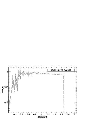
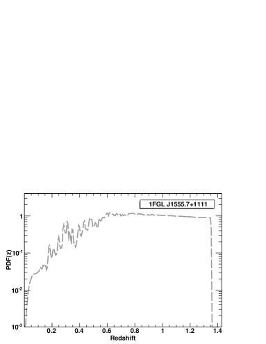
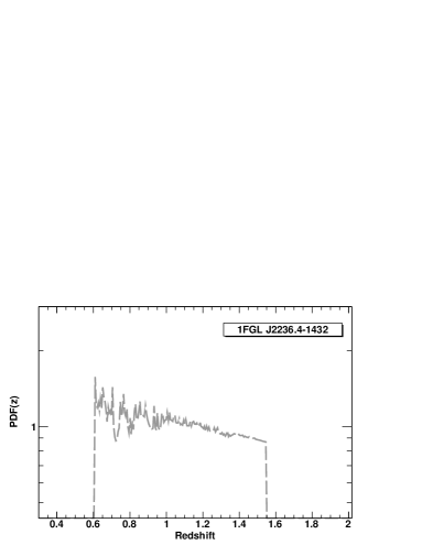
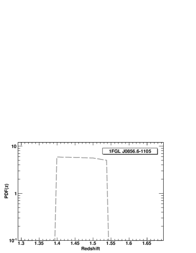
We combine these constraints to produce, for each object, the observationally allowed probability density function (PDF) for the source redshift. However, for the LF analysis we need the redshift PDF, subject to these observational constraints, for the source as a representative member of the Fermi-detected BL Lacs. Accordingly, we assume a prior function that represents the $dN/dz$ distribution if one could measure the spectroscopic redshift for all the BL Lacs in our Fermi sample. This is multiplied by the observational PDF to derive the final PDF for each Fermi-detected BL Lac. If, for example, only $z_{\rm min}$ and $z_{\rm max}$ constraints were available for a given source, its final PDF would follow the prior $dN/dz$ between these limits. As noted below, the prior has only a mild effect on the luminosity function. For each source, then, the PDF is obtained as:

$${\rm PDF}(z)=\frac{dN}{dz}\cdot\prod_{i}^{n}C_{i}(z)$$ (21)

where the $C_{i}(z)$ are the redshift constraints available for that source. Sample PDFs are shown in Fig. 1.

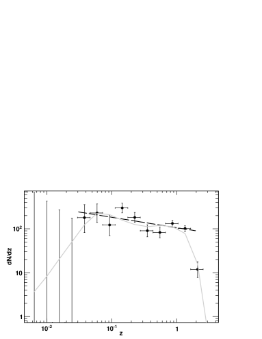
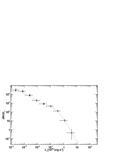
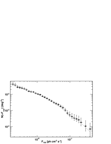
Drawing possible redshifts from these final PDFs for each source, we compute the sample LF as described above and then use this to predict the observed $dN/dz$ using Eq. 6, which represents the redshift distribution expected if all sources could have spectroscopic redshift measurements. In general, this will differ from the initial assumed prior. We replace the prior with this predicted $dN/dz$ and iterate to convergence. Since the $dN/dz$ distribution is rather flat in the range $0.02<$z$<$2, we find that the initially assumed prior has very little effect. In practice we find robust convergence to the same final LF for an initial prior $dN/dz\propto z^{-t}$ with $-0.3<t<0.6$. In all cases the derived distribution shows a clear drop in the number of observed BL Lacs at $z>2$ (see below). However, as this may be an important evolutionary effect that we wish to measure without bias, we conservatively assume a $dN/dz\propto z^{-t}$ prior extending to all $z$ allowed by the constraints. We adopt a computation with an initial $t=0.2$ prior which is shown in the upper left panel of Fig. 2.

Figure 1: Examples of probability density functions (PDFs) for the redshifts of 4 sources. The upper plots show the case of sources with upper limits (spectroscopic and photometric respectively in the left and right plots) coupled to exclusion probabilities and a prior function as discussed in $\S$ 3.3. The bottom panels show the case of sources with both spectroscopic lower limits and photometric upper limits. Both PDFs were combined (as above) with the exclusion probabilities and the prior function.

3.4 Summary of the Analysis Chain

We use a Monte Carlo approach in order to derive the LF and its uncertainty. The steps of the analysis are as follows:

1. An initial prior function (see $\S$ 3.3) is chosen to approximate the $dN/dz$ distribution of the Fermi BL Lacs.

2. We then create 1000 samples of 206 BL Lacs whose redshifts are extracted at random from the PDF of each source. The 206 BL Lacs are drawn with replacement from the objects reported in the Appendix.

3. We use the ML method described in $\S$ 3.1 with one of the parametrizations in $\S$ 3.2 to derive the best-fit LF. This is done independently for each Monte Carlo. The final LF is built as the average of the Monte Carlo LFs and its uncertainty takes into account the spread of all the Monte Carlo LFs. This allows us to quantify naturally the uncertainty in the LF due to the sample size and the spread in the redshift measurements. The LF is used to predict the observed $dN/dz$ through Eq. 5.

4. The $dN/dz$ is compared to the prior function used at step 1): if the two functions are different, then a new prior function based on the latest $dN/dz$ (step 3) is created and substituted to the one of step 1).

5. Steps 1-4 are repeated until the prior and the predicted $dN/dz$ are compatible with each other.

We note that a change in the prior function causes a change in the redshift PDFs of all sources, and thus new PDFs have to be created and the entire analysis (steps 2-4) has to be repeated.

4 Results

In this section we present results on the best-fitting LF models. Particular attention is given to whether adding the $\beta$ and $\tau$ parameters (representing respectively the luminosity-dependent photon index and a luminosity-dependent speed of evolution, see Eq. 11 and 14) significantly improves the quality of the fit.

4.1 Density and Luminosity Evolution

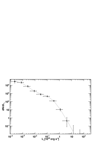
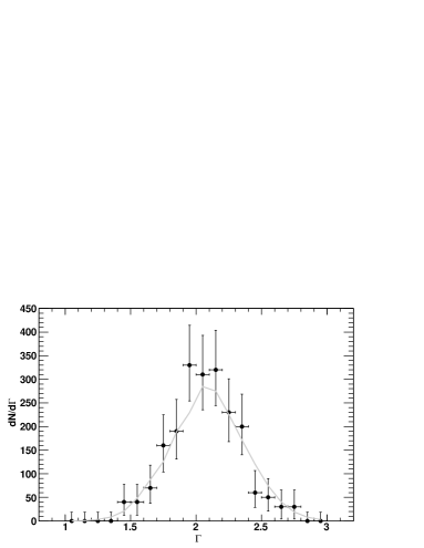
Tab. 2 reports the results of the best fits using a PDE or a PLE parametrization, including cases for which $\beta$ and $\tau$ are allowed to vary. Both the PLE and PDE LFs provide adequate representations of the Fermi data when $\beta$ and $\tau$ are allowed to vary (see PLE₃ and PDE₃ models in Tab. 2). In all cases the PLE model provides a better representation of the Fermi data than the PDE model as indicated by the value of the log-likelihood ($S$ in Eq: 4). As shown in Fig. 2, the best-fit PLE model (model PLE₃ in Tab. 2) reproduces accurately the distribution in luminosity, redshift, photon index and source counts of the Fermi blazars. The model PLE₃ provides the best representation of the LF of BL Lacs.

The improvement in the log-likelihood when $\beta$ and $\tau$ are allowed to vary can be used to quantify the improvement of the fit with the standard formula TS= - 2(ln L₀ - ln L₁), where $L_{1}$ is the hypothesis tested again the null one (L₀) and TS is the likelihood test statistic. We find that allowing the parameter $\beta$ to vary produces an improvement in the fit of TS$>$10 (see Tab. 2) which corresponds to $>3$ $\sigma$ for the case of one additional degree of freedom. The $\tau$ parameter which governs the speed of the evolution as a function of luminosity produces an improvement in the fit of TS=52 ($\sim$7.2 $\sigma$) for the PLE and TS=12 ($\sim$3.4 $\sigma$) for the PDE model.

If we take the luminosities of 10⁴⁵, 10⁴⁶, and 10⁴⁷ erg s^-1 as reference luminosities for the Fermi populations of HSPs, ISPs and LSPs then we find that the redshift peaks of the luminosity evolution are respectively z_c=0.5, 0.8, and 1.2 for these three luminosities. The maximum-likelihood value of the speed of the evolution (parameter $k_{d}$) also changes from 4.7 to 5.8 and 7.0, respectively. It thus seems clear that the evolution depends on the luminosity class.

Figure 2: Observed redshift (upper left), luminosity (upper right), photon index (lower left), and source count (lower right) distributions of LAT BL Lacs. The continuous solid line is the best-fit PLE model convolved with the selection effects of Fermi. The error bars reflect the statistical uncertainty including (for the upper plots) the uncertainty in the sources’ redshifts. Error bars compatible with zero are 1 $\sigma$ upper limits for the case of observing zero events in a given bin (see Gehrels, 1986). The dashed line in the redshift distribution shows one of the prior functions used in $\S$ 3.3.

Table 2: Best-fit parameters of the Pure Luminosity and Pure Density Evolution LFs. Parameters without an error estimate were kept fixed during the fit. Parameter values were computed as the median of all the best-fit parameters to the Monte Carlo sample, while the uncertainties represent the 68 % containment regions around the median value.

Model	A	$\gamma_{1}$	L∗	$\gamma_{2}$	k	$\tau$	$\xi$	$\mu^{*}$	$\beta$	$\sigma$	-2$\ln$L
PLE1	$7.29^{+31.80}_{-7.13}\times 10^{3}$	$1.26^{+0.08}_{-0.20}$	$1.42^{+89.33}_{-0.94}\times 10^{-2}$	$1.31^{+1.78}_{-0.09}$	$4.87^{+0.78}_{-5.39}$	$0$	$-0.48^{+3.48}_{-0.08}$	$2.15^{+0.03}_{-0.03}$	$0$	$0.27^{+0.02}_{-0.02}$	-$690.1$
PLE2	$2.89^{+30.91}_{-2.70}\times 10^{3}$	$1.22^{+0.09}_{-0.42}$	$2.16^{+73.16}_{-1.67}\times 10^{-2}$	$1.37^{+2.10}_{-0.14}$	$4.61^{+0.75}_{-5.13}$	$0$	$-0.48^{+3.48}_{-0.10}$	$2.12^{+0.03}_{-0.03}$	$6.48^{+2.28}_{-2.09}\times 10^{-2}$	$0.26^{+0.02}_{-0.02}$	-$699.9$
PLE3	$9.68^{+6.88}_{-4.75}\times 10^{2}$	$1.47^{+0.14}_{-0.12}$	$4.48^{+2.32}_{-1.20}\times 10^{-2}$	$4.45^{+1.08}_{-0.93}$	$5.89^{+0.99}_{-0.95}$	$1.18^{+0.16}_{-0.22}$	$-0.31^{+0.05}_{-0.06}$	$2.11^{+0.03}_{-0.03}$	$6.47^{+2.23}_{-2.40}\times 10^{-2}$	$0.26^{+0.03}_{-0.02}$	-$752.1$
PLEno-z	9.12${}^{+0.90}_{-0.60}\times 10^{5}$	2.07$\pm 0.52$	0.12$\pm 0.22$	0.77$\pm 0.67$	8.60$\pm 1.07$	1.41$\pm 0.33$	-0.17$\pm 0.04$	2.19$\pm 0.04$	0.16$\pm 0.04$	0.30$\pm 0.04$	$\cdots$
PDE1	$78.53^{+906.10}_{-73.82}$	$1.32^{+18.68}_{-0.10}$	$0.58^{+3.01}_{-0.47}$	$1.25^{+0.09}_{-0.08}$	$11.47^{+1.44}_{-1.94}$	$0$	$-0.21^{+0.02}_{-0.04}$	$2.15^{+0.03}_{-0.03}$	$0$	$0.27^{+0.02}_{-0.02}$	-$695.8$
PDE2	$62.22^{+989.87}_{-55.53}$	$1.32^{+18.68}_{-0.10}$	$1.10^{+2.34}_{-1.01}$	$1.24^{+0.07}_{-0.07}$	$10.72^{+1.50}_{-2.23}$	$0$	$-0.24^{+0.03}_{-0.06}$	$2.12^{+0.03}_{-0.03}$	$6.33^{+2.31}_{-2.00}\times 10^{-2}$	$0.26^{+0.03}_{-0.02}$	-$711.9$
PDE3	$18.78^{+65.86}_{-14.69}$	$3.43^{+0.78}_{-0.42}$	$0.38^{+0.46}_{-0.17}$	$1.56^{+0.16}_{-0.12}$	$16.69^{+3.52}_{-2.77}$	$3.23^{+0.85}_{-0.79}$	$-0.11^{+0.02}_{-0.02}$	$2.10^{+0.03}_{-0.03}$	$6.45^{+2.31}_{-2.31}\times 10^{-2}$	$0.26^{+0.02}_{-0.03}$	-$724.8$

4.2 Luminosity-Dependent Density Evolution

Given the clear luminosity dependence of the evolution found in the previous section we try to fit the LDDE model of $\S$ 3.2. This model has two additional parameters with respect to the PLE and PDE models. The fit with $\tau$=0 (all luminosity classes evolve in the same way) already provides a representation of the data which is as good as the best-fit PLE model (see Tab. 3). If we allow $\tau$ to vary the fit improves further with respect to the baseline LDDE₁ model (TS=30, i.e. $\sim$5.5 $\sigma$). Figure 3 shows how the LDDE₃ model reproduces the observed distributions.

The improvement of the LDDE₂ model with respect to the PLE₃ model can be quantified using the Akaike information criterion (AIC, Akaike, 1974; Wall & Jenkins, 2012). For each model, one can define the quantity $AIC_{i}=2n_{par}-2lnL$ where $n_{par}$ is the number of free parameters and $-2lnL$ is twice the log-likelihood value as reported in Tab. 2 and 3. The relative likelihood of a model with respect to another one can be evaluated as $p=e^{0.5(AIC_{min}-AIC_{i})}$ where $AIC_{min}$ comes from the model providing the minimal $AIC$ value. According to this test the PLE₃ model has a relative likelihood with respect to the LDDE₂ model of $\sim$0.0024. Thus, the model LDDE₂ whose parameters are reported in Tab. 3 fits the Fermi data better ($\sim$3 $\sigma$) than the PLE₃ model.

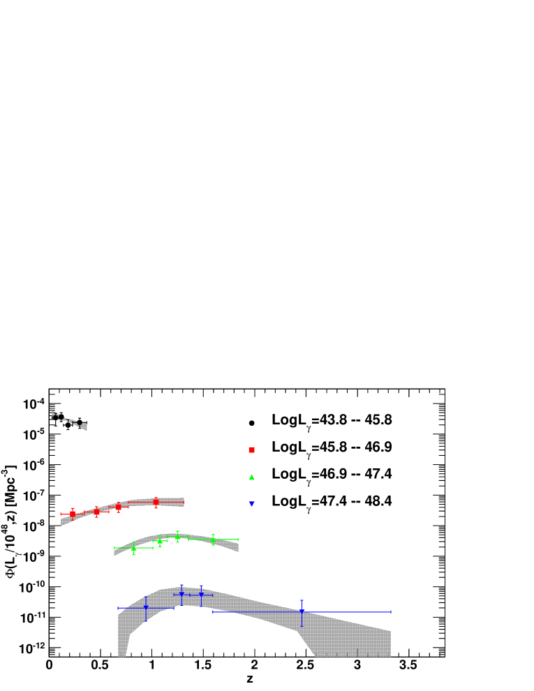
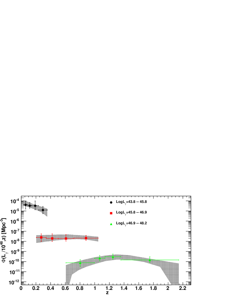
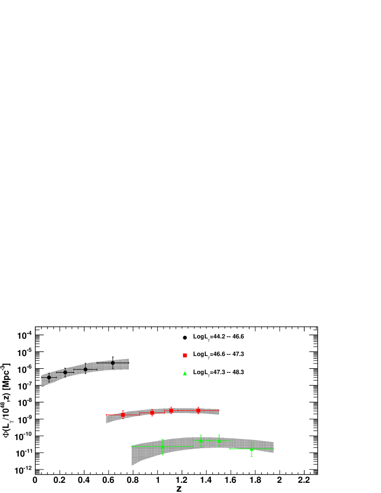
In this representation low-luminosity (L_γ=10⁴⁴ erg s^-1) sources are found to evolve negatively ($p1$=-7.6). On the other hand high-luminosity (L_γ=10⁴⁷ erg s^-1) sources are found to evolve positively ($p1$=7.1). Both evolutionary trends are correctly represented also in the best-fit PLE model (PLE₃ in Tab. 2), but the LDDE model provides a slightly better representation of the data. The different evolution of low-luminosity and high-luminosity sources can be readily appreciated in Fig. 4 which shows the space density of different luminosity classes of BL Lacs as a function of redshift. This figure was created taking into account the dispersion in both redshift and luminosity introduced by the uncertainty in the redshift of many of our BL Lacs. A noteworthy fact is that the least-luminous BL Lacs are 10³ times more numerous than the least luminous FSRQs detected by Fermi (see Fig. 4 in Ajello et al., 2012). The data points were deconvolved with the method described in $\S$ 3.1 (see Eq. 9) while the LF is displayed as the region enclosing 68 % of all the best-fit LDDE models to the 1000 Monte Carlo samples.

The local LF is the luminosity function at redshift zero. For an evolving population, the local LF is obtained by de-evolving the luminosities (or the densities) according to the best-fit model. We follow two approaches to derive the local LF. First, we de-evolve the luminosities using the 1/V_MAX method of Schmidt (1968) but weighting the maximum volume (V_MAX) by the density evolution implied (for a given source luminosity) by our best-fit LDDE model. Following Della Ceca et al. (2008) and Ajello et al. (2012), the maximum allowed volume for a given source is defined as:

$$V_{\rm MAX}=\int^{z_{max}}_{z_{min}}\Omega(L_{i},z,\Gamma)\frac{e(z,L_{i})}{e(z_{min},L_{i})}\frac{dV}{dz}dz$$ (22)

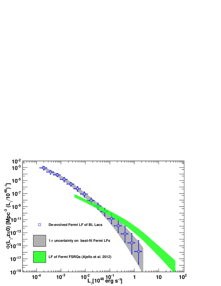
where $L_{i}$ is the source luminosity, $\Omega(L_{i},z,\Gamma)$ is the sky coverage, $z_{max}$ is the redshift above which the source drops out of the survey, and $e(z,L_{i})$ is the evolution term of Eq. 13 normalized (through $e(z_{min},L_{i})$) at the redshift $z_{min}$ to which the LF is to be de-evolved. The LF de-evolved at $z_{min}$ ($z_{min}$=0 in this case) is built using the standard 1/V_MAX method (Schmidt, 1968). This is reported (data points) in Fig. 5. To estimate the uncertainties that different methods might introduce in the local LF we also extrapolated to $z=0$ from the best-fit LDDE models to all the Monte Carlo samples to measure the 68 % range for the local LF. This is shown in Fig. 5 as a gray band. It is apparent that the two methods give consistent results.

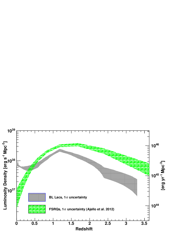
The local LF is found to have a rather steep power law ($dN/dL\propto L^{-3.5}$) down to luminosities of 10⁴⁶ erg s^-1, flattening ($dN/dL\propto L^{-2.0}$) below this value. Because of their steeper local LF and their lower luminosity, BL Lacs reach higher densities than FSRQs (whose local LF is shown for comparison in Fig. 5). Fig. 6 shows the evolution of the luminosity density of BL Lacs compared to that of FSRQs. With their larger luminosity, FSRQs dominate at all redshifts $z>0.3$. Yet the extreme growth in BL Lac numbers at low $z$ allows them to produce $>$10⁴⁵ erg yr^-1 Mpc^-3, or $\sim 90$% of the local luminosity density.

Table 3: Best-fit parameters of the LDDE LFs. Parameters without an error estimate were kept fixed during the fit. Parameter values were computed as the median of all the best-fit parameters to the Monte Carlo sample, while the uncertainty represent the 68 % containment region around the median value.

Model	A	$\gamma_{1}$	L∗	$\gamma_{2}$	z${}_{c}^{*}$	p1∗	$\tau$	p2	$\alpha$	$\mu^{*}$	$\beta$	$\sigma$	-2$\ln$L
LDDE1	$9.20^{+20.60}_{-8.77}\times 10^{2}$	$1.12^{+0.13}_{-0.16}$	$2.43^{+2.25}_{-1.30}$	$3.71^{+16.29}_{-2.39}$	$1.67^{+0.14}_{-0.10}$	$4.50^{+0.75}_{-0.61}$	$0.0$	$-12.88^{+3.66}_{-2.12}$	$4.46^{+6.47}_{-5.24}\times 10^{-2}$	$2.12^{+0.03}_{-0.03}$	$6.04^{+2.15}_{-2.02}\times 10^{-2}$	$0.26^{+0.02}_{-0.02}$	$-734.1$
LDDE2	$3.39^{+7.44}_{-2.13}\times 10^{4}$	$0.27^{+0.26}_{-0.46}$	$0.28^{+0.43}_{-0.21}$	$1.86^{+0.86}_{-0.48}$	$1.34^{+0.22}_{-0.27}$	$2.24^{+1.25}_{-1.07}$	$4.92^{+1.45}_{-2.12}$	$-7.37^{+2.95}_{-5.43}$	$4.53^{+4.98}_{-6.52}\times 10^{-2}$	$2.10^{+0.03}_{-0.03}$	$6.46^{+2.34}_{-2.07}\times 10^{-2}$	$0.26^{+0.02}_{-0.02}$	$-764.6$
LDDEnoProb	1.04${}^{+14.90}_{-0.74}\times 10^{4}$	0.58${}^{+0.18}_{-0.75}$	0.50${}^{+0.75}_{-0.47}$	1.99${}^{+1.70}_{-0.70}$	1.18${}^{+0.38}_{-0.27}$	2.30${}^{+2.11}_{-1.17}$	4.62${}^{+5.38}_{-1.73}$	-4.30${}^{+2.07}_{-4.50}$	8.62${}^{+5.55}_{-13.30}\times 10^{-2}$	2.11${}^{+0.03}_{-0.03}$	6.64${}^{+1.84}_{-2.05}\times 10^{-2}$	0.26${}^{+0.02}_{-0.02}$	$-985$

Figure 3: Observed redshift (upper left), luminosity (upper right), photon index (lower left), and source count (lower right) distributions of LAT BL Lacs. The continuous solid line is the best-fit LDDE model convolved with the selection effects of Fermi. The error bars reflect the statistical uncertainty including (for the upper plots) the uncertainty in the sources’ redshifts. Error bars consistent with zero represent 1 $\sigma$ upper limits for the case of observing zero events in a given bin (see Gehrels, 1986).

Figure 4: Growth and evolution of BL Lacs, separated by luminosity class. The gray bands represent 68 % confidence regions around the best fitting LDDE LF model (for each Monte Carlo sample). Both data points and band errors include uncertainties for the source redshifts as well as statistical uncertainty. All but the least luminous class have a redshift peak near z$\approx$1.5; the lowest luminosity BL Lacs increase toward z=0.

Figure 5: Local (z=0) LF as derived from the best-fit LDDE model ($\S$ 4.2). BL Lacs dominate the local luminosity function for $L_{\gamma}<10^{46}$  erg s^-1. The gray band represents the confidence region enclosing 68 % of the realizations of the best-fit LF to the Monte Carlo samples.

Figure 6: Luminosity density as a function of redshift produced by the Fermi BL Lacs. The gray band represents the confidence region enclosing 68 % of the realizations of the best-fit LF to the Monte Carlo samples.

4.3 The Effect of Neglecting Redshift Constraints

Neglecting redshift constraints and relying only on spectroscopic redshifts reduces the completeness of our sample to only $\sim$48 %. As we show in the following this has dramatic effects on the reliability of the luminosity function.

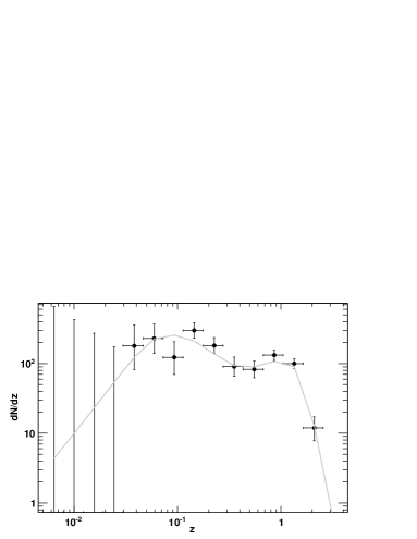
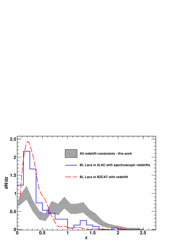
The main reason is that the distribution of spectroscopic redshifts approximates poorly the redshift distribution of BL Lacs inferred using all the redshift constraints presented in $\S$ 3.3. This can clearly be seen in Fig. 7 which compares the BL Lac redshift distribution taking all constraints into account compared to known BL Lac redshift distributions based solely on spectroscopic redshifts. These latter are biased to find low redshift BL Lacs, while it is clear from recent works (Rau et al., 2012; Shaw et al., 2013a, b; Furniss et al., 2013) that there is a relevant population of BL Lacs at intermediate (z$\approx$0.5–1.5) redshift. This is not a spurious effect caused by any of the techniques presented in $\S$ 3.3, but an evidence that comes from all of them. In order to test this, we removed the exclusion probabilities from the used constraints and re-derived the LF. The exclusion probability is available for all but 5 BL Lacs without redshift and on average constrains a given object to be at z$\gtrsim$0.3-0.5. If wrong, it might artificially push the average redshift of BL Lacs to higher values. We find this is not the case. Indeed, even removing the exclusion probabilities the redshift distribution of BL Lacs still shows an increase at z$>0.5$ which is this time mostly due to the redshift lower limits. Moreover as reported in Tab. 3, the LF derived from discarding only the exclusion probabilities (see model LDDE_noProb) is still in agreement with the best-fitting model (LDDE₂) that relies on all constraints.

As expected from the above discussion if we neglect all redshift constraints and rely only on the 103 BL Lacs with spectroscopic redshifts, the best-fit LF (reported as model PLE_no-z in Tab. 2) changes fairly dramatically with respect to the best fit LDDE₂ model. Indeed, instead of showing a change in the evolution with source luminosity, it displays a very mild positive evolution for all luminosity classes. This would lead to a biased estimate of the evolution of BL Lacs. We thus believe that results based on BL Lac samples with scarce redshift coverage are unreliable.

Figure 7: Redshift distribution of Fermi’s BL Lac derived using all constraints of $\S$ 3.3 compared to spectroscopic redshift distributions of BL Lacs in the 2LAC catalog (Ackermann et al., 2011) and the Roma blazar catalog (BZCAT, Massaro et al., 2009). The gray band encloses the 68 % of all realizations of the redshift distribution of the Monte Carlo samples.

4.4 The Intrinsic Luminosity Function of BL Lac Objects

Beaming is known to alter the shape of the intrinsic luminosity function (e.g., Urry & Shafer, 1984; Urry & Padovani, 1991). In this Section we correct for this effect, recovering the intrinsic luminosity function of the Fermi BL Lacs and their Lorentz and Doppler factor distributions. Here we adopt the formalism and symbols already used in Ajello et al. (2012).

The observed 0.1–100 GeV luminosities $L$ defined in the present work are apparent isotropic luminosities (expressed in erg s^-1). Since the jet material is moving at relativistic speed, the observed, Doppler boosted, luminosities are related to the intrinsic values by:

$$L=\delta^{p}\mathscr{L}$$ (23)

where $\mathscr{L}$ is the intrinsic (unbeamed) luminosity and $\delta$ is the kinematic Doppler factor

$$\delta=\left(\gamma-\sqrt{\gamma^{2}-1}\cos\ \theta\right)^{-1}$$ (24)

where $\gamma=(1-\beta^{2})^{-1/2}$ is the Lorentz factor, $\beta=v/c$ is the velocity of the emitting plasma and $\theta$ is the angle between the line of sight and the jet axis. We will assume that our sources have Lorentz factors $\gamma$ in the range $\gamma_{a}\leq\gamma\leq\gamma_{b}$. Then the minimum Doppler factor is $\delta_{min}=\gamma_{b}^{-1}$ (when $\theta$=90^∘) and the maximum is $\delta_{max}=(\gamma_{a}+\sqrt{\gamma_{a}^{2}-1})^{-1}$ (when $\theta=0^{\circ}$). We adopt a value of $p$=4 which is appropriate if the observed emission is dominated by the SSC component of ejected plasma blobs and discuss also the case of $p=3$ which applies to the case of continuous jet emission.

We define the intrinsic luminosity function as:

$$\Phi(\mathscr{L})=k_{1}\mathscr{L}^{-B}$$ (25)

valid in the $\mathscr{L}_{1}\leq\mathscr{L}\leq\mathscr{L}_{2}$ range. The joint probability of observing a beamed luminosity $L$ and Doppler factor $\delta$ is (see also Lister, 2003):

$$P(L,\delta)=P_{\delta}(\delta)\cdot\Phi(\mathscr{L})\frac{d\mathscr{L}}{dL}$$ (26)

where $P_{\delta}(\delta)$ is the probability density for the Doppler $\delta$ and $d\mathscr{L}/dL$=$\delta^{-p}$. Assuming a random distribution for the jet angles (i.e. $P_{\theta}=\sin\ \theta$), this results in

$$P_{\delta}(\delta)=\int P_{\gamma}(\gamma)P_{\theta}(\theta)\left|\frac{d\theta}{d\delta}\right|d\gamma=\int P_{\gamma}(\gamma)\frac{1}{\gamma\delta^{2}\beta}d\gamma,$$ (27)

since

$$\left|\frac{d\theta}{d\delta}\right|=\frac{1}{sin(\theta)\delta^{2}\sqrt{\gamma^{2}-1}}=\frac{1}{sin(\theta)\delta^{2}\gamma\beta}$$ (28)

From here it follows that

$$P_{\delta}(\delta)=\delta^{-2}\int^{\gamma_{b}}_{f(\delta)}\frac{P_{\gamma}(\gamma)}{\sqrt{\gamma^{2}-1}}\ d\gamma$$ (29)

where $P_{\gamma}(\gamma)$ is the probability density for $\gamma$ and the lower limit of integration $f(\delta)$ depends on the Doppler factor value and is reported in Eq. A6 in Lister (2003). Integrating over $\delta$ yields the observed luminosity function of the Doppler beamed BL Lacs:

$$\Phi(L)=k_{1}L^{-B}\int^{\delta_{2}(L)}_{\delta_{1}(L)}P_{\delta}(\delta)\delta^{p(B-1)}d\delta$$ (30)

where, as in Cara & Lister (2008), the limits of integration are

$$\delta_{1}(L)={\rm min}\{\delta_{max},{\rm max}\left(\delta_{min},(L/\mathscr{L}_{2})^{1/p}\right)\}$$ (31)

$$\delta_{2}(L)={\rm max}\{\delta_{min},{\rm min}\left(\delta_{max},(L/\mathscr{L}_{1})^{1/p}\right)\}$$ (32)

In this way, by fitting Eq. 30 to the Fermi Doppler boosted LF, it is possible to determine the parameters of the intrinsic luminosity function and of the Lorentz-factor distribution.

We assume that the probability density distribution for $\gamma$ is a power law of the form

$$P_{\gamma}(\gamma)=C\gamma^{k}$$ (33)

where C is a normalization constant and the function is valid for $\gamma_{a}\leq\gamma\leq\gamma_{b}$. We set the largest intrinsic luminosity $\mathscr{L}_{2}=10^{4}\mathscr{L}_{1}$, but this choice has hardly any impact on the results. Fits with parameters similar to those of FSRQs ($p=4$, $\gamma_{a}=5$, $\gamma_{b}=40$ and $\mathscr{L}_{1}=10^{40}$ erg s^-1) are ruled out ($\chi^{2}$/dof $>$2.5). In order to obtain acceptable fits we find that $\mathscr{L}_{1}$ has to be set to $\leq 10^{40}$ erg s^-1 or $\leq 10^{38}$ erg s^-1 for the $p=3$ and $p=4$ case respectively. Moreover, in agreement with the observation of BL Lacs in radio (e.g. Lähteenmäki & Valtaoja, 2003; Lister et al., 2009; Savolainen et al., 2010), we set $\gamma_{a}=2$ which is lower than the minimum value used (and found) for FSRQs (see e.g. Ajello et al., 2012). In order to allow for a population of highly beamed BL Lacs we set $\gamma_{b}=90$.

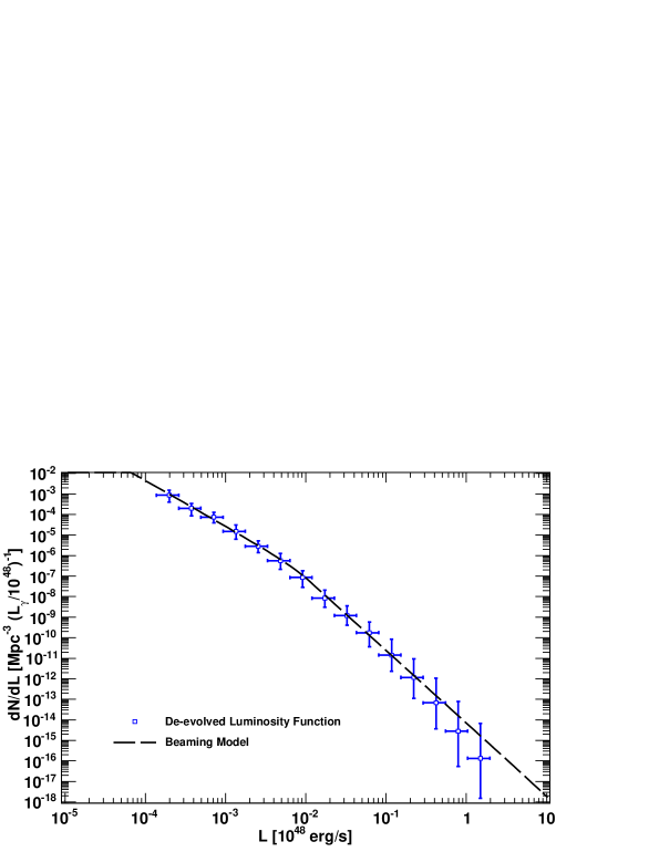
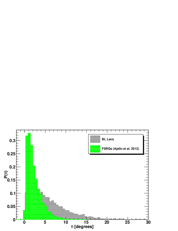
The free parameters of the problem are the normalization ($k_{1}$) and, the slope ($B$) of the intrinsic LF and the slope $k$ of the Lorentz factor distribution. We have fitted Eq. 30 to the Fermi LF de-evolved at redshift zero derived in $\S$4.2. Fig. 8 shows how the best-fit beaming model reproduces the local LF of BL Lacs measured by Fermi. For the $p=4$ case we can use the fit values to derive an intrinsic LF slope of $B=3.30\pm 0.30$ and a Lorentz-factor distribution index of $k=-2.32\pm 0.51$. The parameters for the $p=3$ case are similar. Our distribution of Lorentz factors is somewhat steeper than (but compatible with, within the uncertainties) that found by Lister & Marscher (1997) who report a slope of $-1.75<k<-1.5$. The fit values are summarized in Table 4. The Lorentz-factor distributions (for the $p=3$ and $p=4$ cases) imply an average Lorentz factor $\gamma\approx 6$ for the detected Fermi blazars. This is in agreement with past inferences for radio and X-ray selected BL Lacs (see discussion in Urry & Padovani, 1995; Morganti et al., 1995). The average Lorentz-factor depends on the value adopted for $\gamma_{a}$ (and to lesser extent on $\gamma_{b}$). Within the errors, the slope $k$ is the same for BL Lacs and FSRQs ($-2.32\pm 0.51$ versus $-2.03\pm 0.70$ respectively). The fact that it is not possible to produce a good fit to the data adopting the same $\gamma_{a}$ for both populations implies that a population of BL Lacs exists with jets slower than those of FSRQs. This yields a smaller value for the average Lorentz factor ($\gamma^{BL\ Lac}\approx 6$ versus $\gamma^{FSRQ}\approx 12$) and that BL Lacs are seen under larger angles ($\sim$5 ^∘ versus $\sim$2 ^∘ for FSRQs, see Fig. 9).

Finally, we also tested different parametrizations of the distribution of Lorentz factors (Eq. 33). We used a linear, an exponential, and a Gaussian distribution. None of these models provides an acceptable fit to the data ($\chi^{2}/dof>3$). We thus conclude that parametrizing the Lorentz factor distribution with a power-law model (as done also in the literature, e.g. Urry & Shafer, 1984; Cara & Lister, 2008) is a reasonable assumption.

Table 4: Parameters of the beaming models described in the text. Parameters without an error estimate were kept fixed during the fitting stage.

Parameter	Value	Value
$k$	-2.26$\pm 0.20$	-2.32$\pm 0.51$
$k_{1}$	4.3$\pm 0.5$	2.7$\pm 0.5$
$B$	3.96$\pm 0.08$	3.30$\pm 0.30$
$\gamma_{a}$	2	2
$\gamma_{b}$	90	90
$\mathscr{L}_{1}$	1040	1038
$\mathscr{L}_{2}$	1044	1042
$p$	3	4
$\chi^{2}/dof$	0.3	0.21
Average $\gamma$	6.1${}^{+1.1}_{-0.8}$	5.8${}^{+3.6}_{-1.6}$

Figure 8: Fermi’s LF de-evolved at redshift zero and best-fit beaming model (for $p$=4, dashed line, see text) described in $\S$ 4.4.

Figure 9: Normalized distributions of viewing angles with respect to the jet axis for Fermi BL Lacs and FSRQs.

5 Sub-classes of BL Lac Objects

Our sample can be subdivided into 96 HSPs, 64 ISPs and 45 LSPs on the basis of the frequency of the synchrotron peak (see Ackermann et al., 2011). For only 6 objects there is not enough multiwavelength coverage to define accurately the position of the synchrotron peak. It is thus possible to test whether the different sub-classes of BL Lacs have different evolution. In particular we are interested in testing the following two scenarios: 1) whether HSPs have a different evolution with respect to ISPs and LSPs, and 2) whether LSPs have a different evolution with respect to HSPs and ISPs. For completeness the best-fit parameters of all the models described in $\S$ 5.1 and 5.2 are reported in the Appendix ($\S$ A.2).

5.1 The Evolution of HSP Objects

Using the same best-fit models (namely the PLE and LDDE models of $\S$ 3.2) we next examine separately the HSP objects. The LDDE model is slightly preferred to the PLE model (TS$\approx$12). Both models indicate that the evolution of the HSP is negative: i.e. the density is growing with decreasing redshift.

For the PLE model, the relevant parameters are: $k=3.82^{+1.29}_{-1.17}$, $\tau=1.35^{+0.17}_{-0.32}$, and $\gamma=-0.40^{+0.07}_{-0.14}$. For all the HSPs with L${}_{\gamma}\leq$10⁴⁶ erg s^-1 the evolution is negative $z_{c}\leq 0$ and $k_{d}\leq$0. The same trend is confirmed by the LDDE model whose relevant parameters are $p1^{*}=0.48^{+1.63}_{-0.48}$, and $\tau=6.76^{+2.33}_{-1.82}$ (see Eq. 20).

For the class of ISP and LSP objects the LDDE model produces a very small improvement over the PLE model (TS$\approx$3). Both models indicate positive evolution for the ISPs and LSPs considered together. For the PLE, the parameters that govern the evolution are: $k=7.86^{+1.41}_{-1.86}$, $\tau=0.98^{+0.28}_{-0.31}$, and $\xi=-0.25^{+0.05}_{-0.08}$. In this scenario low-luminosity sources are characterized by a slow positive evolution consistent with no evolution.

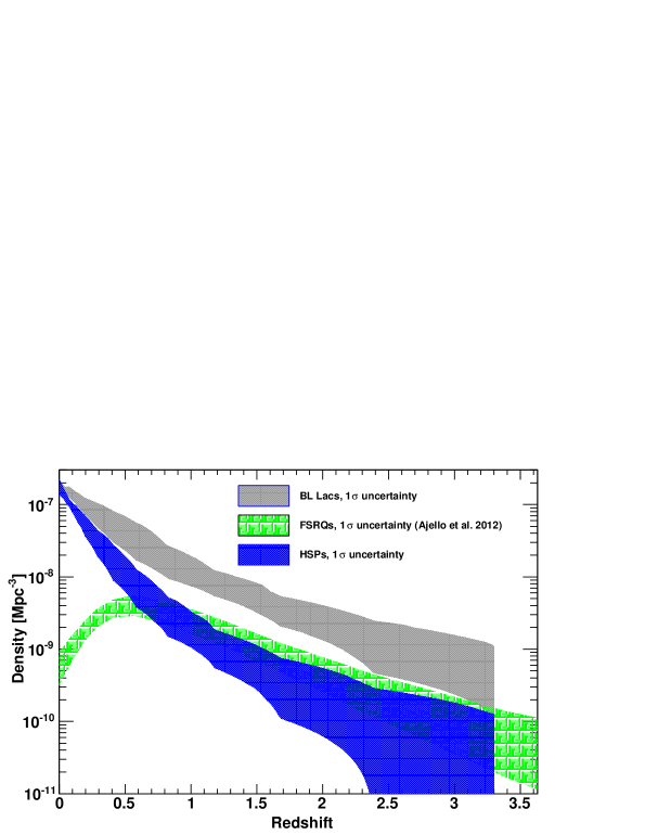
The different evolutionary behavior of HSPs with respect to all other blazar classes can be appreciated in Fig. 10 which shows that the dramatic rise in the number density of BL Lacs at z$\leq$1 is driven almost entirely by the HSP population. The fact that low-luminosity HSP objects are the only ones experiencing negative evolution can also be seen directly in Fig. 11.

Figure 10: Number density (per unit co-moving volume) of BL Lacs, FSRQs and HSPs.

Figure 11: Evolution of different luminosity classes of HSPs (top) and ISPs+LSPs (bottom). Note the different evolutionary behavior (negative for HSPs versus positive for ISPs+LSPs evolution) of low-luminosity sources.

5.2 The Evolution of LSP Objects

LSP objects are the class of BL Lac objects that most closely resemble the FSRQ class. Their synchrotron component peaks at frequencies $<10^{14}$ Hz (Ackermann et al., 2011), they can show rather large values of the Compton dominance (Finke, 2013), and their average redshift is larger than that of the rest of BL Lacs. A number of LSPs might be FSRQs whose jet is aligned along our line-of-sight and whose non-thermal radiation reduces the equivalent width of optical lines. Indeed, Shaw et al. (2013b) find that many BL Lac sources (especially LSPs) are spectrally classified as FSRQ when seen in low states. Since the FSRQ class is known to evolve positively (Ajello et al., 2012), the close connection between FSRQs and high luminosity BL Lacs might be responsible for the positive evolution detected for the high-luminosity objects in $\S$ 4.2.

The model that best describes the LF of LSP objects is the PLE model. The best-fit evolutionary parameters of the PLE model ($k=7.59^{+1.78}_{-2.09}$, $\tau=1.30^{+0.26}_{-0.39}$, and $\xi=-0.23^{+0.05}_{-0.08}$) imply a strong positive evolution for LSP objects of all luminosities as it is the case for FSRQs (see e.g. Ajello et al., 2012).

The LDDE model applied to HSPs and ISPs yields: p${}_{1}^{*}=1.98^{+1.46}_{-1.20}$, and $\tau=6.38^{+1.58}_{-1.66}$. These parameters are in agreement with those of the full sample (reported in Tab. 3 and imply negative evolution for low-luminosity objects (L${}_{\gamma}\leq$10⁴⁶ erg s^-1) and positive evolution for high-luminosity objects (L${}_{\gamma}>$10⁴⁶ erg s^-1).

For high-luminosity BL Lacs (L${}_{\gamma}\sim$10⁴⁷ erg s^-1) both models described above find a positive evolution with $k_{d}\approx 8.9$ (for the PLE model) and p${}_{1}\approx 8-9$ (for the LDDE). As such it is apparent that LSPs are not driving the positive evolution of the whole BL Lac sample, but that this is a characteristic of all high-luminosity BL Lacs.

6 Discussion and Conclusions

In this work we determined the first luminosity function of GeV-detected BL Lacs. This was made possible by the relatively complete redshift information gleaned from a variety of methods (see e.g. Rau et al., 2012; Shaw et al., 2013b), leaving only 5 of our 211 BL Lacs without redshift constraints. Previous BL Lac samples selected at other frequencies contained few objects (often $<$50) and typically lacked redshift information for $\geq$30 % of the objects (see e.g. Stickel et al., 1991; Padovani et al., 2007; Marcha & Caccianiga, 2013). Poor redshift completeness renders the luminosity function unreliable (see $\S$ 4.3). Also, our sample contains a substantial number of BL Lacs from each of the three spectral peak subclasses and covers a large redshift range. As such, this sample stands as the largest and most complete (redshift wise) set of BL Lacs ever used at any frequency, and has allowed a greatly improved characterization of the BL Lac population, beaming and evolution. The main results of our analysis are discussed below.

6.1 The Evolution of the BL Lac Luminosity Function

In the past, BL Lacs have been found to show a wide range of evolutionary patterns. Rector et al. (2000), Giommi et al. (1999), and Beckmann et al. (2003) (whose samples contained large fractions of HSP objects) found the BL Lacs to evolve negatively, Caccianiga et al. (2002) and Padovani et al. (2007) found that BL Lacs do not evolve, and recently Marcha & Caccianiga (2013) reported on a sample with positive evolution. These different results were likely due to limited statistics and inadequate redshift coverage mixed with selection of different classes of BL Lacs.

As clear from this work, the evolution of the BL Lac class is complex. We found that the evolution of BL Lac objects selected by Fermi can be described with a LDDE model similar to the one used for FSRQs (Ajello et al., 2012). Indeed, luminous BL Lacs ($\sim$10⁴⁷ erg s^-1) evolve as strongly ($p_{1}\sim 7$) as FSRQs (see $\S$ 4.2). However, the evolution of BL Lacs slows down with luminosity, becoming negative for objects with L${}_{\gamma}\leq$10^45.5 erg s^-1.

Subdividing the sample in HSP, ISP and LSP objects we find that the negative evolution is in fact isolated to the HSP population, while the ISP and LSP evolve positively from the lowest luminosities. Our analysis thus confirms results based on samples dominated by HSP objects (e.g. Giommi et al., 1999; Beckmann et al., 2003). We tested if different slopes of the luminosity function (Eq. 12) respectively for HSPs and ISPs+LSPs could be compatible with a common (e.g. positive) shape of the evolution. We find that, while it seems HSPs have a slightly flatter luminosity function (at redshift $\approx$0) than ISPs+LSPs, imposing a common shape of the evolution to the whole population substantially worsen the fit (by $\sim$10 $\sigma$). On the other hand, allowing HSPs and ISPs+LSPs to have different evolutions reproduces the negative-positive dichotomy. We can also exclude that the negative evolution scenario is caused by inadequate redshift coverage (incompleteness), or by the fact that HSPs are not detected to sufficiently large redshifts (sensitivity limit). Indeed, from our set of Monte Carlo simulations we find that $~{}\sim$30 % and $~{}\sim$7 % of all the HSPs detected by Fermi lie respectively at z$>1$ and z$>1.5$. Moreover, the effect of the extragalactic background light (EBL, see $\S$ 6.2) is not severe and does not bias either the measured fluxes or the photon indices in the 0.1–100 GeV band. In order to exclude that the negative evolution of low-luminosity BL Lacs (and HSPs) is caused by the incompleteness of the sample used here (see $\S$ 2), we explore a worst case scenario assuming that all $\sim$20 unassociated sources are BL Lacs lying in the 0.2–0.7 redshift range. A large population of BL Lacs at intermediate redshifts (z$\sim$0.5, see left panel of Fig. 11) would be needed to invert the negative evolution. Using actual fluxes and photon indices drawn from the 23 unclassified possible AGN, assuming that all are HSP and drawing random redshifts in the critical 0.2-0.7 range, we find that only a relatively small fraction ($\sim$12 %) could be HSPs with Log L${}_{\gamma}<$45.5. Accordingly, even in this worst-case scenario we find that these missing identifications cannot significantly alter our measurement of negative evolution for this sub-class.

The slowing down of the evolution with decreasing source luminosity has been observed in many kinds of AGN, including the population of radio galaxies (Longair, 1966; Schmidt, 1972; Willott et al., 2001), but an inversion of the evolution at very low luminosity as observed here is difficult to interpret. While the close connection between the FSRQ and LSP classes is quite apparent, it is less obvious that this trend can be extended to the HSP BL Lacs. However, one may interpret this spectral sequence as a progression caused by the gradual depletion of an AGN’s gas reservoir via accretion (e.g. Cavaliere & D’Elia, 2002; Böttcher & Dermer, 2002). In this context a LSP object would transition from disk-powered jet production (at high accretion rates) through the ISP class to an HSP BL Lac object with low accretion rates and a radiatively inefficient accretion flow. In LSPs, strong cooling due to the circumnuclear radiation fields would limit the maximum energy reached by the accelerated electrons. For the HSPs, due to the decreased cooling efficiency, particles would be accelerated to much larger energies which would translate into a peak frequency of the synchrotron component that moves from 10¹³ Hz up to 10¹⁷ Hz. This reproduces the paradigm of the blazar sequence (Ghisellini et al., 1998; Fossati et al., 1998).

The activity of FSRQs, if triggered by galaxy merging events as is common for high-luminosity quasars, would be short lived ($\tau\sim$0.1 Gyr), and be followed by the low-accretion regime of HSP-type BL Lacs which can be sustained for much longer times ($\tau\sim$5–7 Gyr Cavaliere & D’Elia, 2002). In the high-redshift Universe, where gas was abundant, galaxy merging favors the activity of FSRQs. As the Universe expands, galaxy merging becomes infrequent and most of the FSRQs/LSPs finish consuming their fuel reserve, transitioning to a long-lasting low accretion regime. If the HSPs are indeed starved LSP objects then one should observe an increase in the space density of BL Lacs with only a slight lag (since $\tau\sim$0.1 Gyr for FSRQs) from the decrease in the space density of FSRQs. Fig. 10 can been seen as supporting this picture. Indeed at z$\geq$1.5 the number density of HSPs decreases in a similar way to that of FSRQs and LSPs and ISPs objects. At z$<$0.5 when the FSRQs turn off, the space density of HSPs, and in particular the low luminosity HSP, quickly increases.

This scenario is attractive but still speculative. At present we lack a quantitative comparison between the space densities of the FSRQ+LSP objects and the (possibly remnant) population of HSP. Certainly different beaming characteristics ( and their potential evolution with redshift) can affect the estimated populations and complicate this comparison. There may also be differences between the low and high-peaked sources in the typical black hole mass or host galaxy environment. Nevertheless, the correlation of opposing evolutionary trends found here points to a possible connection between these AGN populations.

6.2 Softening of Blazar Spectra with Redshift

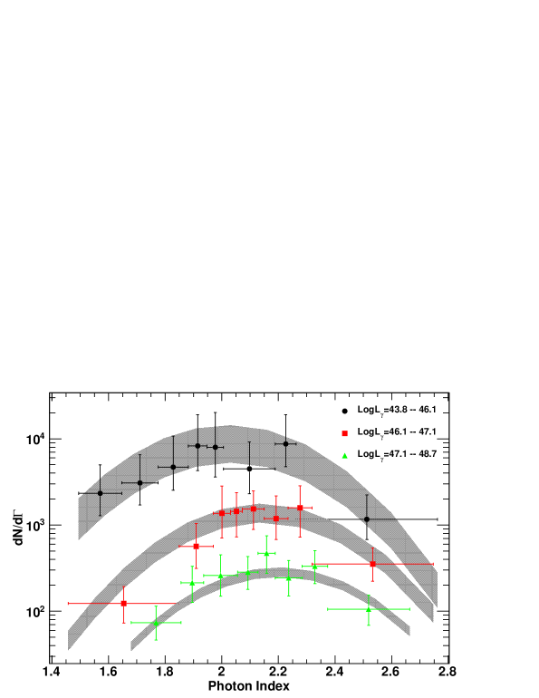
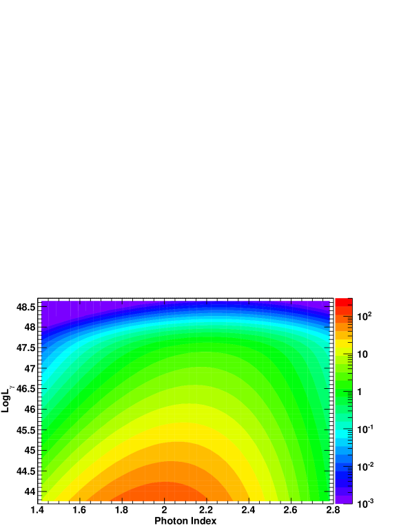
In $\S$ 4.1 and 4.2 we found that Fermi blazar spectra soften with increasing luminosity. In particular, all the best-fit models have BL Lac spectra softening at high luminosity. The average photon index changes from $\sim$2.0 to $\sim$2.2 when the luminosity changes from 10⁴⁴ erg s^-1 to 10⁴⁸ erg s^-1.

The left panel of Fig. 12 shows the deconvolved intrinsic photon index distributions for three different luminosity classes. The deconvolution was performed with the method outlined in $\S$ 3.1 (see Eq. 9). The y-axis reports the integral over redshift and luminosity of Eq. 1 (essentially $dN/d\Gamma$). The trend of the average softening of the BL Lac spectra with increasing luminosity is apparent even though the dynamic range is small: i.e. the index changes by only $\Delta\Gamma\approx 0.2$ in 4 orders of magnitudes in luminosity. The right panel of Fig. 12 shows the photon index-luminosity plane as predicted by the best-fit LF. The correlation of the photon index with luminosity is very clear. Both of these figures include corrections for all known selection effects, so we infer that this trend is directly apparent in the sources (although it is strongly amplified in the observed sample through selection effects).

If selection effects are not properly taken into account, a spurious index-luminosity correlation can be artificially introduced because of the energy dependence of the Fermi-LAT point-spread function (Atwood et al., 2009) which favors the detection at low fluxes of sources with a hard spectrum (see Fig. 1 in Abdo et al., 2010c). However, the analysis of the source count distribution as a function of photon index did not reveal any significant correlation between flux and photon index (Abdo et al., 2010c; Singal et al., 2012).

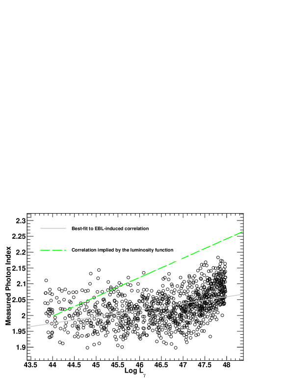
Finally, a spurious luminosity-index correlation might be produced by absorption of high-energy photons by the EBL. The EBL attenuation would make measured spectra steeper than intrinsic, preferentially affecting high-redshift (and thus high-luminosity) sources. We checked to see if this produced the observed trend, by simulating $\sim$1000 spectra in the 0.1–100 GeV band using a power-law model with a photon index of 2.0. Fluxes and redshifts were drawn from the observed sample of BL Lacs and EBL absorption was applied using models (Franceschini et al., 2008; Finke et al., 2010; Domínguez et al., 2011) in agreement with Fermi observations of the EBL attenuation (Ackermann et al., 2012). The result of this analysis, reported in Fig. 13, shows that the EBL effect on measured photon indices (in the 0.1–100 GeV band) is minor. While the photon index of BL Lacs with Log L${}_{\gamma}>$47.5 erg s^-1 is modified by the EBL attenuation by $\Delta\Gamma\sim$0.055, the index of all sources below that luminosity is basically unaffected. Thus, we conclude that the observed index-luminosity correlation is not an artifact of selection effects or cosmic EBL absorption, but intrinsic to the sources.

Ghisellini et al. (2009) was the first to note (although without accounting for selection effects) that a correlation between index and $\gamma$-ray luminosity seemed to exist for BL Lacs and FSRQs detected by Fermi. They proposed that the 0.1–100 GeV luminosity of 10⁴⁷ erg s^-1 which separates hard BL Lacs from soft FSRQs could be associated with a transition in the accretion flow from radiatively inefficient (e.g. Narayan et al., 1997) to optically-thick radiatively efficient (Shakura & Sunyaev, 1973).

The picture seems to be slightly more complex. FSRQs stand as a monolithic population for which there is no correlation between photon index and luminosity (Ajello et al., 2012). This is likely due to the fact that at GeV energies their spectrum is dominated by the external Compton emission (Dermer & Schlickeiser, 1993). On the other hand, the index-luminosity correlation for BL Lacs as argued above has a significant intrinsic component. This points towards the fact that particles in luminous BL Lacs cool more efficiently than in low-luminosity objects, in agreement with the results of Finke (2013) who finds an anti-correlation between the Compton dominance and the frequency at the peak of the synchrotron component.

The correlation between index and luminosity reported by Ghisellini et al. (2009) is much stronger than that which we find here ($\Delta\Gamma$/$\Delta{\rm Log}L_{\gamma}\sim$0.25 versus $\sim$0.06); this was thus likely dominated by the uncorrected selection effects. It does not seem to be the case that luminous and hard BL Lacs exist in such numbers to destroy the correlation as suggested by Giommi et al. (2013), although a few such objects are indeed seen in our sample. Hard luminous BL Lacs exist (see Fig. 12), as predicted by the Fermi best-fit luminosity function, but they are rare, representing the tail of the $dN/dL_{\gamma}d\Gamma$ distribution.

Figure 12: Top Panel: Deconvolved index distribution for three luminosity classes of Fermi BL Lacs. Note the shift in the average of the distribution with luminosity. Bottom Panel: Deconvolved photon index-luminosity plane for the Fermi BL Lacs (in units of number of BL Lacs per bin of luminosity and index).

Figure 13: Measured photon index versus measured luminosity for a sample of 1000 power-law spectra (with $\Gamma$=2) with fluxes and redshifts randomly drawn from the sample of BL Lacs used here. An EBL attenuation using the model of Franceschini et al. (2008) was applied to all the spectra. The measured quantities (index, flux and luminosity) were derived fitting source spectra with a power law. The solid line shows the best linear fit to the observed data points. The dashed line shows the correlation between photon index and luminosity found by the best-fit LDDE model in $\S$ 4.2.

6.3 The Contribution to the Isotropic Gamma-Ray Background

This analysis has important consequences for the understanding of the isotropic gamma-ray background (IGRB, Fichtel et al., 1975; Sreekumar et al., 1998; Abdo et al., 2010b) whose origin is still unclear (Abdo et al., 2010c; Ajello et al., 2012).

A simple integration of the luminosity function yields the diffuse emission arising from the unresolved BL Lac class (in the 0.1–100 GeV band) as 8.0${}^{+2.0}_{-1.3}\times 10^{-7}$ ph cm^-2 s^-1 sr^-1, which represents 7.7${}^{+2.0}_{-1.3}$ % of the intensity measured by Fermi. The slightly disfavored PLE model predicts that BL Lacs produce 1.07${}^{+0.21}_{-0.17}\times 10^{-6}$ ph cm^-2 s^-1 sr^-1 and thus 10.3$\pm 2$ % of the IGRB. It thus seems clear that BL Lacs do not account for more than $\sim$10–15 % of the IGRB.

While this might seem to represent a small number, the large density of hard sources present in the nearby Universe, as predicted by the luminosity function makes the spectrum of the diffuse emission arising from the BL Lac class harder than that of the IGRB. Since this depends on the assumed spectral models for different BL Lac classes and on the EBL model, the actual contribution from the common extreme HSP sources may be larger. The exact energy-dependent derivation is left to a future publication.

7 Summary

This work relies on a complete sample of 211 BL Lacs, detected by Fermi during its first year of operations, to deepen our knowledge of this elusive, yet very important, blazar population. Our findings can be summarized as follows:

• The typical redshift completeness of any BL Lac sample is $<$50 %. The Fermi sample is no exception with only 103 BL Lacs (out of 211) having a spectroscopic redshift measurement. Using four different techniques (described in Sec. 3.3) we were able to provide quantitative constraints on the redshift of an additional 104 objects making this the largest and most complete sample of BL Lacs available in the literature. We find that most of the objects without a spectroscopic redshift (and thus $\sim$half of the BL Lac population) lie at z$>$0.5–0.7 which is larger than the typical spectroscopic limit reached for BL Lacs.

• Independently of the functional form used to represent the data, we find that the BL Lac population displays (as found for other classes of AGN) a speed of evolution which depends on luminosity, with high-luminosity sources evolving faster than low-luminosity ones. The negative evolution (i.e. more BL Lacs at lower than higher redshifts) of the low-luminosity BL Lacs is a major result of this work. We find that HSPs are certainly responsible for most, if not all, of the detected negative evolution. This confirms previous claims of negative evolution based on samples of X-ray selected BL Lacs, which contained a large fraction of HSPs (Rector et al., 2000; Beckmann et al., 2003).

• This work allows us to explore the link between the BL Lac and the FSRQ families of blazars. The local (z$\approx$0) luminosity function of BL Lac overlaps and connects smoothly to that of FSRQs, highlighting the similarity between the two classes with BL Lacs having on average lower luminosity (and thus very likely lower Lorentz factors) than FSRQs. This last aspect is confirmed by the analysis of the intrinsic luminosity function which allows us, using a simple beaming model, to derive the distributions of Lorentz factors and of viewing angles. FSRQs and BL Lacs have a similar distribution of Lorentz factors (i.e. a power-law distribution with index $\approx-$2.5), but the one of BL Lacs extends to slower jet speeds implying that the jets of BL Lacs are, on average, seen under larger angles than those of FSRQs ($\sim$5 ^∘ for BL Lacs versus $\sim$2 ^∘ for FSRQs).

• One of the most interesting finding of this work is the evidence supporting the genetic link between FSRQs and BL Lacs as proposed by Cavaliere & D’Elia (2002) and Böttcher & Dermer (2002). In this scenario BL Lacs represent the final (gas starved, inefficiently accreting) and long-lasting phase of an earlier, short-lived, merger-driven gas-rich epoch (the FSRQ). The sudden increase in the space density of BL Lacs (driven in particular by the HSPs) at the same epoch as the turn off of FSRQs corroborates the idea of a transition from the FSRQ to the BL Lac class. To investigate further the details of this transition would require, for both classes, a robust beaming correction and knowledge of the black hole mass and host galaxy environment, which are at present not well constrained.

• The study of the luminosity function shows that the spectra of BL Lacs at GeV energies soften with increasing luminosity even after correcting for the substantial selection effects. The effect is not as dramatic as reported in the literature (e.g. Ghisellini et al., 2009), but might still be caused by the fact that particles in luminous BL Lacs cool more efficiently than in low-luminosity objects.

• Unresolved BL Lacs contribute $\sim$10–15 % of the IGRB measured by Fermi (Abdo et al., 2010b). However, the large density of hard sources at low redshift, as implied from the luminosity function derived in this work, will certainly increase the contribution of BL Lacs to the IGRB at $>10$ GeV. A confirmation of this is already available in the study of the $>10$ GeV sources detected by Fermi (Ackermann et al., 2013).

Appendix A Appendix

A.1 Table with Redshift Constraints

Table 5 reports the 211 BL Lacs used in this work with all the available redshift constraints (with the exception of the exclusion functions). The sample and the nature of the redshift constraints are described in $\S$ 2 and $\S$ 3.3.

Table 5: The 211 BL Lac Objects detected by Fermi used for this analysis. The nature of the redshift constraints is described in $\S$ 3.3.

NAME	Flux100	Photon Index	z	photo-z	zLL	zMAX	photo-zUL	SED CLASS
1FGL J0006.9+4652	4.35$\pm 0.79$	2.50$\pm 0.12$	$\cdots$	$\cdots$	$\cdots$	$\cdots$	$\cdots$	ISP
1FGL J0021.7-2556	1.22$\pm 0.41$	2.13$\pm 0.16$	$\cdots$	$\cdots$	0.56	1.63	1.44	ISP
1FGL J0022.2-1850	0.45$\pm 0.16$	1.64$\pm 0.13$	$\cdots$	$\cdots$	0.77	1.64	1.38	HSP
1FGL J0033.5-1921	2.03$\pm 0.32$	1.89$\pm 0.07$	$\cdots$	$\cdots$	0.50	1.77	$\cdots$	HSP
1FGL J0035.1+1516	0.70$\pm 0.23$	1.72$\pm 0.12$	$\cdots$	1.28	$\cdots$	1.65	$\cdots$	HSP
1FGL J0038.0+1236	1.41$\pm 0.59$	2.23$\pm 0.19$	0.089	$\cdots$	$\cdots$	1.76	$\cdots$	HSP
1FGL J0045.3+2127	1.39$\pm 0.38$	1.86$\pm 0.11$	$\cdots$	$\cdots$	$\cdots$	1.78	1.06	HSP
1FGL J0050.6-0928	7.39$\pm 0.64$	2.20$\pm 0.05$	0.635	$\cdots$	$\cdots$	2.18	$\cdots$	ISP
1FGL J0100.2+0747	1.90$\pm 0.36$	1.90$\pm 0.09$	$\cdots$	$\cdots$	$\cdots$	4.01	$\cdots$	ISP/HSP
1FGL J0105.7+3930	4.80$\pm 0.90$	2.70$\pm 0.14$	0.440	$\cdots$	$\cdots$	2.68	$\cdots$	$\cdots$
1FGL J0109.0+1816	0.76$\pm 0.35$	2.00$\pm 0.19$	0.443	$\cdots$	$\cdots$	2.48	$\cdots$	HSP
1FGL J0114.4+1327	3.81$\pm 0.76$	2.66$\pm 0.14$	$\cdots$	$\cdots$	$\cdots$	1.63	1.22	ISP/HSP
1FGL J0115.5+2519	1.49$\pm 0.42$	2.02$\pm 0.12$	$\cdots$	$\cdots$	0.27	1.63	1.45	HSP
1FGL J0115.7+0357	1.19$\pm 0.40$	2.03$\pm 0.15$	0.913	$\cdots$	0.14	1.62	1.25	$\cdots$
1FGL J0120.5-2700	3.90$\pm 0.45$	2.03$\pm 0.06$	$\cdots$	$\cdots$	0.56	1.76	$\cdots$	ISP
1FGL J0136.5+3905	2.86$\pm 0.39$	1.80$\pm 0.06$	$\cdots$	$\cdots$	$\cdots$	1.65	$\cdots$	HSP
1FGL J0141.7-0929	1.85$\pm 0.45$	2.16$\pm 0.12$	0.735	$\cdots$	0.50	2.17	$\cdots$	ISP
1FGL J0144.6+2703	4.77$\pm 0.65$	2.22$\pm 0.08$	$\cdots$	$\cdots$	0.71	1.66	$\cdots$	ISP
1FGL J0154.1+0823	1.68$\pm 0.39$	1.97$\pm 0.10$	0.681	$\cdots$	0.34	1.64	1.37	ISP
1FGL J0155.0+4433	0.95$\pm 0.55$	2.10$\pm 0.23$	$\cdots$	$\cdots$	0.39	1.63	$\cdots$	ISP/HSP
1FGL J0158.0-3931	2.19$\pm 0.52$	2.34$\pm 0.14$	$\cdots$	$\cdots$	$\cdots$	2.15	1.35	ISP
1FGL J0159.5+1047	1.28$\pm 0.19$	1.95$\pm 0.06$	0.195	$\cdots$	$\cdots$	1.76	$\cdots$	HSP
1FGL J0159.7-2741	0.98$\pm 0.30$	2.06$\pm 0.14$	$\cdots$	$\cdots$	0.58	1.78	1.05	ISP
1FGL J0203.5+3044	4.91$\pm 0.85$	2.74$\pm 0.13$	0.761	$\cdots$	$\cdots$	2.72	$\cdots$	$\cdots$
1FGL J0209.3-5229	1.80$\pm 0.48$	1.94$\pm 0.11$	$\cdots$	$\cdots$	$\cdots$	2.18	1.18	HSP
1FGL J0210.6-5101	14.63$\pm 0.95$	2.37$\pm 0.04$	0.999	$\cdots$	$\cdots$	$\cdots$	$\cdots$	ISP
1FGL J0211.2+1049	3.86$\pm 0.69$	2.27$\pm 0.09$	$\cdots$	$\cdots$	$\cdots$	1.67	$\cdots$	ISP
1FGL J0213.2+2244	1.29$\pm 0.40$	1.95$\pm 0.13$	0.459	$\cdots$	$\cdots$	2.66	$\cdots$	HSP
1FGL J0217.9-6630	1.19$\pm 0.46$	2.07$\pm 0.17$	$\cdots$	$\cdots$	0.67	1.88	1.25	HSP
1FGL J0222.6+4302	21.51$\pm 1.03$	1.94$\pm 0.02$	$\cdots$	$\cdots$	$\cdots$	1.67	$\cdots$	ISP
1FGL J0238.6+1637	43.54$\pm 1.10$	2.15$\pm 0.02$	0.940	$\cdots$	$\cdots$	$\cdots$	$\cdots$	ISP
1FGL J0238.6-3117	0.96$\pm 0.35$	2.07$\pm 0.17$	0.232	$\cdots$	$\cdots$	1.63	1.02	HSP
1FGL J0250.4+1715	1.28$\pm 0.40$	2.13$\pm 0.13$	0.612	$\cdots$	$\cdots$	$\cdots$	3.10	$\cdots$
1FGL J0303.5-2406	4.71$\pm 0.41$	2.00$\pm 0.05$	0.260	$\cdots$	$\cdots$	$\cdots$	$\cdots$	HSP
1FGL J0315.9-2609	0.32$\pm 0.16$	1.62$\pm 0.17$	0.443	$\cdots$	$\cdots$	$\cdots$	$\cdots$	HSP
1FGL J0316.1+0904	1.73$\pm 0.42$	1.78$\pm 0.09$	$\cdots$	$\cdots$	$\cdots$	1.66	$\cdots$	HSP
1FGL J0319.7+1847	0.51$\pm 0.23$	1.65$\pm 0.16$	0.190	$\cdots$	$\cdots$	$\cdots$	$\cdots$	HSP
1FGL J0322.1+2336	4.26$\pm 0.92$	2.41$\pm 0.12$	$\cdots$	$\cdots$	$\cdots$	$\cdots$	$\cdots$	HSP
1FGL J0323.7-0106	0.34$\pm 0.16$	1.59$\pm 0.17$	0.392	$\cdots$	$\cdots$	2.17	1.54	HSP
1FGL J0326.2+0222	1.94$\pm 0.53$	2.21$\pm 0.13$	0.147	$\cdots$	$\cdots$	$\cdots$	$\cdots$	HSP
1FGL J0334.2-4010	7.85$\pm 0.10$	2.34$\pm 0.01$	1.357	$\cdots$	1.21	2.05	$\cdots$	ISP
1FGL J0334.4-3727	2.59$\pm 0.18$	2.09$\pm 0.04$	$\cdots$	$\cdots$	$\cdots$	1.92	1.34	ISP
1FGL J0354.6+8009	7.76$\pm 0.90$	2.58$\pm 0.08$	$\cdots$	$\cdots$	$\cdots$	$\cdots$	$\cdots$	ISP
1FGL J0416.8+0107	0.80$\pm 0.50$	1.96$\pm 0.24$	0.287	$\cdots$	$\cdots$	$\cdots$	$\cdots$	HSP
1FGL J0428.6-3756	31.07$\pm 0.89$	2.13$\pm 0.02$	1.111	$\cdots$	$\cdots$	$\cdots$	$\cdots$	ISP
1FGL J0434.1-2018	1.67$\pm 0.46$	2.31$\pm 0.15$	0.928	$\cdots$	$\cdots$	2.43	$\cdots$	ISP
1FGL J0448.5-1633	1.05$\pm 0.37$	1.97$\pm 0.15$	$\cdots$	$\cdots$	$\cdots$	1.63	1.25	HSP
1FGL J0449.5-4350	10.40$\pm 0.55$	1.99$\pm 0.03$	0.205	$\cdots$	$\cdots$	$\cdots$	$\cdots$	HSP
1FGL J0507.9+6738	1.37$\pm 0.20$	1.73$\pm 0.06$	0.340	$\cdots$	$\cdots$	2.51	$\cdots$	HSP
1FGL J0509.3+0540	8.18$\pm 0.87$	2.31$\pm 0.06$	0.336	$\cdots$	$\cdots$	1.66	1.24	ISP
1FGL J0516.7-6207	5.56$\pm 0.01$	2.28$\pm 0.00$	1.300	$\cdots$	$\cdots$	1.87	$\cdots$	ISP
1FGL J0536.2-3348	5.54$\pm 0.70$	2.37$\pm 0.08$	$\cdots$	$\cdots$	$\cdots$	2.17	1.16	HSP
1FGL J0538.8-4404	38.22$\pm 1.08$	2.28$\pm 0.02$	0.892	$\cdots$	$\cdots$	$\cdots$	$\cdots$	ISP
1FGL J0543.8-5531	0.97$\pm 0.31$	1.75$\pm 0.12$	0.271	$\cdots$	$\cdots$	2.57	1.08	HSP
1FGL J0616.9+5701	1.63$\pm 0.48$	2.06$\pm 0.13$	$\cdots$	$\cdots$	0.80	3.94	$\cdots$	ISP
1FGL J0617.7-1718	1.14$\pm 0.45$	1.98$\pm 0.15$	0.098	$\cdots$	$\cdots$	1.75	$\cdots$	ISP
1FGL J0700.4-6611	5.61$\pm 0.01$	2.13$\pm 0.00$	$\cdots$	$\cdots$	$\cdots$	1.92	1.46	ISP
1FGL J0706.5+3744	1.82$\pm 0.55$	2.19$\pm 0.14$	$\cdots$	$\cdots$	$\cdots$	1.63	$\cdots$	HSP
1FGL J0707.3+7742	2.48$\pm 0.29$	2.28$\pm 0.06$	$\cdots$	$\cdots$	$\cdots$	1.76	$\cdots$	ISP
1FGL J0710.6+5911	0.24$\pm 0.12$	1.50$\pm 0.18$	0.125	$\cdots$	$\cdots$	$\cdots$	$\cdots$	HSP
1FGL J0711.4+4731	2.91$\pm 0.68$	2.52$\pm 0.14$	1.292	$\cdots$	$\cdots$	$\cdots$	$\cdots$	ISP
1FGL J0712.7+5033	2.86$\pm 0.47$	2.07$\pm 0.08$	0.502	$\cdots$	$\cdots$	1.67	$\cdots$	ISP
1FGL J0721.9+7120	17.39$\pm 0.80$	2.15$\pm 0.03$	$\cdots$	$\cdots$	$\cdots$	2.61	$\cdots$	ISP
1FGL J0738.2+1741	5.08$\pm 0.52$	2.06$\pm 0.05$	$\cdots$	$\cdots$	0.42	1.80	1.30	HSP
1FGL J0752.8+5353	0.88$\pm 0.34$	1.95$\pm 0.16$	0.730	$\cdots$	$\cdots$	1.94	$\cdots$	ISP
1FGL J0757.2+0956	5.30$\pm 0.69$	2.44$\pm 0.08$	0.266	$\cdots$	$\cdots$	$\cdots$	$\cdots$	ISP
1FGL J0804.7+7534	0.71$\pm 0.30$	1.79$\pm 0.15$	0.121	$\cdots$	$\cdots$	$\cdots$	$\cdots$	HSP
1FGL J0809.5+5219	2.07$\pm 0.48$	1.99$\pm 0.11$	0.137	$\cdots$	$\cdots$	2.22	$\cdots$	HSP
1FGL J0811.1-7527	1.39$\pm 0.39$	1.86$\pm 0.11$	$\cdots$	$\cdots$	0.69	1.91	1.40	ISP
1FGL J0811.2+0148	3.58$\pm 0.70$	2.56$\pm 0.13$	1.148	$\cdots$	$\cdots$	$\cdots$	$\cdots$	ISP
1FGL J0815.0+6434	3.10$\pm 0.63$	2.31$\pm 0.11$	0.239	$\cdots$	$\cdots$	1.64	$\cdots$	ISP
1FGL J0818.2+4222	12.19$\pm 0.71$	2.17$\pm 0.04$	$\cdots$	$\cdots$	$\cdots$	2.47	$\cdots$	ISP
1FGL J0825.9+0309	0.51$\pm 0.28$	1.88$\pm 0.21$	0.505	$\cdots$	$\cdots$	3.21	$\cdots$	ISP
1FGL J0831.6+0429	7.18$\pm 0.76$	2.49$\pm 0.07$	0.174	$\cdots$	$\cdots$	2.19	$\cdots$	ISP
1FGL J0844.0+5314	0.51$\pm 0.23$	1.90$\pm 0.18$	$\cdots$	$\cdots$	$\cdots$	2.51	$\cdots$	ISP
1FGL J0847.2+1134	0.23$\pm 0.10$	1.49$\pm 0.16$	0.198	$\cdots$	$\cdots$	2.17	$\cdots$	HSP
1FGL J0854.8+2006	5.37$\pm 0.55$	2.20$\pm 0.06$	0.306	$\cdots$	$\cdots$	$\cdots$	$\cdots$	ISP
1FGL J0856.6-1105	5.70$\pm 0.71$	2.34$\pm 0.07$	$\cdots$	$\cdots$	1.40	2.18	1.54	ISP
1FGL J0902.4+2050	1.65$\pm 0.44$	2.11$\pm 0.13$	$\cdots$	$\cdots$	$\cdots$	2.18	1.21	ISP
1FGL J0905.5+1356	0.90$\pm 0.35$	1.94$\pm 0.16$	$\cdots$	$\cdots$	$\cdots$	1.64	1.35	HSP
1FGL J0910.7+3332	1.69$\pm 0.48$	2.26$\pm 0.14$	0.354	$\cdots$	$\cdots$	1.77	$\cdots$	HSP
1FGL J0915.7+2931	1.67$\pm 0.11$	1.95$\pm 0.03$	$\cdots$	$\cdots$	$\cdots$	1.69	$\cdots$	HSP
1FGL J0945.6+5754	1.50$\pm 0.46$	2.21$\pm 0.15$	0.229	$\cdots$	$\cdots$	2.17	$\cdots$	ISP/HSP
1FGL J0953.0-0838	2.22$\pm 0.40$	1.93$\pm 0.08$	$\cdots$	$\cdots$	$\cdots$	1.64	1.28	HSP
1FGL J1000.9+2915	1.95$\pm 0.43$	2.14$\pm 0.11$	0.558	$\cdots$	$\cdots$	$\cdots$	$\cdots$	ISP
1FGL J1007.9+0619	3.02$\pm 0.70$	2.38$\pm 0.12$	$\cdots$	$\cdots$	$\cdots$	2.17	1.44	ISP
1FGL J1012.2+0634	1.61$\pm 0.76$	2.31$\pm 0.21$	0.727	$\cdots$	0.52	2.16	$\cdots$	ISP
1FGL J1015.1+4927	6.44$\pm 0.48$	1.92$\pm 0.04$	0.212	$\cdots$	$\cdots$	$\cdots$	$\cdots$	HSP
1FGL J1031.0+5051	0.57$\pm 0.23$	1.78$\pm 0.16$	$\cdots$	$\cdots$	$\cdots$	2.17	$\cdots$	HSP
1FGL J1032.7+3737	1.38$\pm 0.42$	2.27$\pm 0.16$	$\cdots$	$\cdots$	0.53	2.17	$\cdots$	ISP
1FGL J1037.7+5711	3.22$\pm 0.47$	2.03$\pm 0.07$	$\cdots$	$\cdots$	$\cdots$	1.64	$\cdots$	ISP
1FGL J1053.6+4927	0.41$\pm 0.14$	1.56$\pm 0.13$	0.140	$\cdots$	$\cdots$	2.17	$\cdots$	HSP
1FGL J1054.5+2212	3.67$\pm 0.13$	2.32$\pm 0.02$	$\cdots$	$\cdots$	$\cdots$	1.64	1.36	ISP
1FGL J1058.1-8006	7.50$\pm 0.43$	2.56$\pm 0.02$	0.581	$\cdots$	$\cdots$	$\cdots$	$\cdots$	ISP
1FGL J1058.4+0134	13.88$\pm 0.07$	2.32$\pm 0.00$	0.888	$\cdots$	$\cdots$	$\cdots$	$\cdots$	ISP
1FGL J1058.6+5628	5.62$\pm 0.53$	2.01$\pm 0.05$	0.143	$\cdots$	$\cdots$	2.18	$\cdots$	HSP
1FGL J1059.3-1132	4.37$\pm 0.02$	2.23$\pm 0.00$	$\cdots$	$\cdots$	$\cdots$	1.65	$\cdots$	ISP
1FGL J1104.4+0734	2.17$\pm 0.56$	2.30$\pm 0.13$	$\cdots$	$\cdots$	$\cdots$	1.65	$\cdots$	ISP/HSP
1FGL J1104.4+3812	17.09$\pm 0.57$	1.81$\pm 0.02$	0.031	$\cdots$	$\cdots$	$\cdots$	$\cdots$	HSP
1FGL J1107.8+1502	0.86$\pm 0.04$	2.01$\pm 0.02$	$\cdots$	$\cdots$	0.60	2.16	$\cdots$	HSP
1FGL J1117.1+2013	1.36$\pm 0.27$	1.77$\pm 0.08$	0.138	$\cdots$	$\cdots$	2.17	$\cdots$	HSP
1FGL J1121.0+4209	0.39$\pm 0.16$	1.64$\pm 0.15$	0.124	$\cdots$	$\cdots$	2.17	$\cdots$	HSP
1FGL J1133.1+0033	2.66$\pm 0.52$	2.15$\pm 0.10$	0.678	$\cdots$	$\cdots$	1.86	$\cdots$	ISP
1FGL J1136.6+7009	1.14$\pm 0.27$	1.87$\pm 0.10$	0.046	$\cdots$	$\cdots$	$\cdots$	$\cdots$	HSP
1FGL J1150.2+2419	2.10$\pm 0.50$	2.28$\pm 0.13$	$\cdots$	$\cdots$	$\cdots$	2.21	$\cdots$	ISP
1FGL J1150.5+4152	1.76$\pm 0.37$	1.93$\pm 0.10$	$\cdots$	$\cdots$	0.85	1.66	$\cdots$	HSP
1FGL J1151.6+5857	1.31$\pm 0.56$	2.23$\pm 0.19$	$\cdots$	$\cdots$	$\cdots$	1.76	$\cdots$	ISP
1FGL J1154.0-0008	0.38$\pm 0.34$	1.72$\pm 0.33$	0.254	$\cdots$	$\cdots$	2.22	$\cdots$	HSP
1FGL J1202.9+6032	2.71$\pm 0.75$	2.44$\pm 0.16$	0.065	$\cdots$	$\cdots$	2.18	$\cdots$	ISP
1FGL J1204.4+1139	1.33$\pm 0.46$	2.23$\pm 0.17$	0.296	$\cdots$	$\cdots$	2.17	$\cdots$	HSP
1FGL J1217.7+3007	5.86$\pm 0.58$	1.98$\pm 0.05$	0.130	$\cdots$	$\cdots$	$\cdots$	$\cdots$	HSP
1FGL J1218.4-0128	1.11$\pm 0.31$	1.96$\pm 0.12$	$\cdots$	$\cdots$	0.64	1.64	1.23	ISP
1FGL J1221.3+3008	2.02$\pm 0.36$	1.76$\pm 0.07$	0.184	$\cdots$	$\cdots$	2.18	$\cdots$	HSP
1FGL J1221.5+2814	8.12$\pm 0.64$	2.09$\pm 0.04$	0.103	$\cdots$	$\cdots$	2.22	$\cdots$	ISP
1FGL J1226.7-1332	0.60$\pm 0.21$	1.74$\pm 0.13$	$\cdots$	$\cdots$	$\cdots$	1.76	1.30	ISP
1FGL J1230.4+2520	1.21$\pm 0.35$	2.07$\pm 0.13$	0.135	$\cdots$	$\cdots$	1.78	$\cdots$	ISP
1FGL J1231.6+2850	2.46$\pm 0.36$	1.94$\pm 0.07$	0.236	$\cdots$	$\cdots$	2.18	$\cdots$	HSP
1FGL J1243.1+3627	1.25$\pm 0.28$	1.79$\pm 0.09$	$\cdots$	$\cdots$	0.48	1.77	$\cdots$	HSP
1FGL J1248.2+5820	6.35$\pm 0.61$	2.17$\pm 0.06$	$\cdots$	$\cdots$	$\cdots$	1.64	$\cdots$	ISP
1FGL J1249.8+3706	0.54$\pm 0.21$	1.80$\pm 0.15$	$\cdots$	$\cdots$	$\cdots$	2.19	$\cdots$	HSP
1FGL J1253.0+5301	3.74$\pm 0.51$	2.13$\pm 0.08$	$\cdots$	$\cdots$	0.66	1.64	$\cdots$	ISP
1FGL J1303.0+2433	4.88$\pm 0.52$	2.17$\pm 0.06$	$\cdots$	$\cdots$	0.77	1.69	$\cdots$	ISP
1FGL J1304.3-4352	3.85$\pm 0.64$	2.06$\pm 0.07$	$\cdots$	$\cdots$	$\cdots$	2.12	1.30	HSP
1FGL J1309.5+4304	1.45$\pm 0.32$	1.94$\pm 0.10$	0.691	$\cdots$	0.69	1.80	$\cdots$	HSP
1FGL J1314.7+2346	1.76$\pm 0.40$	2.10$\pm 0.11$	$\cdots$	$\cdots$	$\cdots$	4.68	1.30	ISP
1FGL J1338.9+1153	1.17$\pm 0.05$	2.08$\pm 0.02$	$\cdots$	1.61${}^{+0.04}_{-0.10}$	1.59	1.94	$\cdots$	ISP
1FGL J1351.5+1115	0.17$\pm 0.02$	1.49$\pm 0.04$	$\cdots$	$\cdots$	0.62	1.64	1.12	HSP
1FGL J1418.3-0235	1.31$\pm 0.33$	1.88$\pm 0.10$	$\cdots$	$\cdots$	$\cdots$	1.64	1.37	HSP
1FGL J1421.0+5421	3.69$\pm 0.88$	2.76$\pm 0.17$	0.153	$\cdots$	$\cdots$	$\cdots$	$\cdots$	ISP
1FGL J1425.0+3614	0.78$\pm 0.39$	2.05$\pm 0.20$	$\cdots$	$\cdots$	$\cdots$	2.17	$\cdots$	ISP
1FGL J1426.9+2347	7.47$\pm 0.49$	1.85$\pm 0.03$	$\cdots$	$\cdots$	$\cdots$	1.66	1.11	HSP
1FGL J1428.7+4239	0.38$\pm 0.17$	1.60$\pm 0.16$	0.129	$\cdots$	$\cdots$	2.18	$\cdots$	HSP
1FGL J1437.0+5640	0.20$\pm 0.12$	1.46$\pm 0.21$	$\cdots$	$\cdots$	$\cdots$	2.08	$\cdots$	HSP
1FGL J1440.9+0613	5.66$\pm 0.85$	2.63$\pm 0.11$	$\cdots$	$\cdots$	0.32	1.63	1.31	ISP
1FGL J1442.8+1158	0.44$\pm 0.26$	1.73$\pm 0.23$	0.163	$\cdots$	$\cdots$	2.17	$\cdots$	HSP
1FGL J1444.0-3906	2.72$\pm 0.45$	1.90$\pm 0.07$	$\cdots$	$\cdots$	$\cdots$	2.20	$\cdots$	HSP
1FGL J1447.9+3608	1.60$\pm 0.39$	1.99$\pm 0.11$	$\cdots$	$\cdots$	0.74	1.76	$\cdots$	HSP
1FGL J1454.6+5125	2.58$\pm 0.53$	2.30$\pm 0.10$	$\cdots$	$\cdots$	$\cdots$	1.63	$\cdots$	ISP
1FGL J1501.1+2237	1.16$\pm 0.26$	1.77$\pm 0.09$	0.235	$\cdots$	$\cdots$	2.18	$\cdots$	HSP
1FGL J1503.5-1544	0.89$\pm 0.45$	1.79$\pm 0.19$	$\cdots$	$\cdots$	0.21	1.76	$\cdots$	HSP
1FGL J1505.1-3435	1.85$\pm 0.73$	2.19$\pm 0.17$	$\cdots$	$\cdots$	1.55	3.13	$\cdots$	ISP
1FGL J1517.8-2423	7.47$\pm 0.83$	2.13$\pm 0.06$	0.048	$\cdots$	$\cdots$	$\cdots$	$\cdots$	ISP
1FGL J1521.0-0350	1.67$\pm 0.50$	2.04$\pm 0.13$	$\cdots$	$\cdots$	0.87	1.80	$\cdots$	HSP
1FGL J1522.6-2732	5.94$\pm 0.84$	2.30$\pm 0.08$	1.294	$\cdots$	$\cdots$	$\cdots$	$\cdots$	ISP
1FGL J1542.9+6129	7.08$\pm 0.62$	2.16$\pm 0.05$	$\cdots$	$\cdots$	$\cdots$	1.76	$\cdots$	ISP
1FGL J1548.7-2250	2.36$\pm 0.85$	2.19$\pm 0.16$	0.192	$\cdots$	$\cdots$	1.65	$\cdots$	HSP
1FGL J1553.5-3116	0.50$\pm 0.21$	1.71$\pm 0.14$	$\cdots$	$\cdots$	$\cdots$	1.97	$\cdots$	HSP
1FGL J1555.7+1111	6.77$\pm 0.45$	1.68$\pm 0.03$	$\cdots$	$\cdots$	$\cdots$	1.77	1.35	HSP
1FGL J1558.9+5627	2.60$\pm 0.75$	2.19$\pm 0.14$	0.300	$\cdots$	1.05	2.47	$\cdots$	ISP
1FGL J1607.1+1552	4.62$\pm 0.66$	2.32$\pm 0.08$	0.496	$\cdots$	$\cdots$	$\cdots$	$\cdots$	ISP
1FGL J1643.5-0646	4.11$\pm 0.86$	2.27$\pm 0.10$	0.082	$\cdots$	$\cdots$	2.07	$\cdots$	HSP
1FGL J1649.6+5241	1.61$\pm 0.48$	2.16$\pm 0.14$	$\cdots$	$\cdots$	$\cdots$	2.47	$\cdots$	$\cdots$
1FGL J1653.9+3945	5.67$\pm 0.45$	1.81$\pm 0.04$	0.034	$\cdots$	$\cdots$	$\cdots$	$\cdots$	HSP
1FGL J1719.2+1745	4.33$\pm 0.52$	2.02$\pm 0.06$	$\cdots$	$\cdots$	$\cdots$	1.64	$\cdots$	ISP
1FGL J1725.0+1151	2.48$\pm 0.50$	1.89$\pm 0.09$	$\cdots$	$\cdots$	$\cdots$	1.65	$\cdots$	HSP
1FGL J1725.5+5854	1.31$\pm 0.35$	2.03$\pm 0.12$	$\cdots$	$\cdots$	$\cdots$	1.66	$\cdots$	ISP
1FGL J1727.9+5010	0.79$\pm 0.33$	1.94$\pm 0.17$	0.055	$\cdots$	$\cdots$	$\cdots$	$\cdots$	HSP
1FGL J1744.2+1934	0.74$\pm 0.32$	1.83$\pm 0.16$	0.083	$\cdots$	$\cdots$	$\cdots$	$\cdots$	HSP
1FGL J1748.5+7004	2.29$\pm 0.20$	2.05$\pm 0.04$	0.770	$\cdots$	$\cdots$	$\cdots$	$\cdots$	ISP
1FGL J1749.0+4323	2.39$\pm 0.10$	2.09$\pm 0.02$	$\cdots$	$\cdots$	0.57	1.65	$\cdots$	ISP
1FGL J1751.5+0937	11.15$\pm 1.37$	2.32$\pm 0.06$	0.322	$\cdots$	$\cdots$	$\cdots$	$\cdots$	ISP
1FGL J1754.3+3212	3.06$\pm 0.53$	2.10$\pm 0.09$	$\cdots$	$\cdots$	$\cdots$	1.63	$\cdots$	HSP
1FGL J1800.4+7827	6.11$\pm 0.04$	2.35$\pm 0.00$	0.684	$\cdots$	$\cdots$	$\cdots$	$\cdots$	ISP
1FGL J1807.0+6945	6.33$\pm 0.89$	2.53$\pm 0.09$	0.051	$\cdots$	$\cdots$	$\cdots$	$\cdots$	ISP
1FGL J1809.6+2908	1.20$\pm 0.47$	2.07$\pm 0.16$	$\cdots$	$\cdots$	$\cdots$	1.63	$\cdots$	ISP
1FGL J1811.0+1607	3.35$\pm 0.69$	2.22$\pm 0.10$	$\cdots$	$\cdots$	$\cdots$	1.74	$\cdots$	ISP
1FGL J1813.4+3141	2.77$\pm 0.49$	2.11$\pm 0.09$	0.117	$\cdots$	$\cdots$	$\cdots$	$\cdots$	ISP
1FGL J1824.0+5651	6.55$\pm 0.73$	2.36$\pm 0.07$	0.664	$\cdots$	$\cdots$	2.48	$\cdots$	ISP
1FGL J1829.8+5404	1.96$\pm 0.71$	2.39$\pm 0.19$	$\cdots$	$\cdots$	$\cdots$	2.46	$\cdots$	HSP
1FGL J1832.6-5700	2.40$\pm 0.74$	2.22$\pm 0.15$	$\cdots$	$\cdots$	1.23	1.96	$\cdots$	HSP
1FGL J1838.6+4756	1.09$\pm 0.36$	1.92$\pm 0.13$	$\cdots$	$\cdots$	$\cdots$	$\cdots$	$\cdots$	HSP
1FGL J1849.6-4314	2.04$\pm 0.56$	2.17$\pm 0.13$	$\cdots$	$\cdots$	$\cdots$	1.94	$\cdots$	ISP/HSP
1FGL J1903.0+5539	2.93$\pm 0.46$	1.97$\pm 0.07$	$\cdots$	$\cdots$	0.73	1.63	$\cdots$	ISP
1FGL J1918.4-4108	2.06$\pm 0.42$	1.91$\pm 0.09$	$\cdots$	$\cdots$	1.59	2.11	$\cdots$	ISP
1FGL J1926.8+6153	2.76$\pm 0.55$	2.13$\pm 0.10$	$\cdots$	$\cdots$	$\cdots$	1.65	$\cdots$	HSP
1FGL J1936.9-4720	0.73$\pm 0.36$	1.82$\pm 0.18$	0.265	$\cdots$	$\cdots$	$\cdots$	$\cdots$	HSP
1FGL J1958.4-3013	2.07$\pm 0.82$	2.23$\pm 0.17$	0.119	$\cdots$	$\cdots$	$\cdots$	$\cdots$	HSP
1FGL J2000.0+6508	7.22$\pm 0.67$	2.05$\pm 0.05$	0.049	$\cdots$	$\cdots$	$\cdots$	$\cdots$	HSP
1FGL J2006.0+7751	3.14$\pm 0.91$	2.44$\pm 0.16$	0.342	$\cdots$	$\cdots$	$\cdots$	$\cdots$	ISP
1FGL J2009.1+7228	4.32$\pm 1.15$	2.58$\pm 0.15$	$\cdots$	$\cdots$	1.74	2.03	$\cdots$	ISP
1FGL J2009.5-4849	3.87$\pm 0.49$	1.88$\pm 0.06$	0.071	$\cdots$	$\cdots$	$\cdots$	$\cdots$	HSP
1FGL J2015.3-0129	2.26$\pm 0.62$	2.19$\pm 0.13$	$\cdots$	$\cdots$	$\cdots$	1.78	1.22	ISP
1FGL J2016.2-0903	2.21$\pm 0.01$	2.18$\pm 0.00$	$\cdots$	$\cdots$	0.60	1.63	$\cdots$	ISP
1FGL J2031.5+1219	4.11$\pm 0.04$	2.42$\pm 0.01$	1.213	$\cdots$	0.85	$\cdots$	$\cdots$	ISP
1FGL J2039.0-1047	2.80$\pm 0.12$	2.18$\pm 0.02$	$\cdots$	$\cdots$	$\cdots$	1.63	$\cdots$	ISP
1FGL J2131.7-0914	0.88$\pm 0.39$	1.97$\pm 0.18$	0.449	$\cdots$	$\cdots$	$\cdots$	$\cdots$	HSP
1FGL J2139.3-4235	9.71$\pm 0.69$	2.12$\pm 0.04$	$\cdots$	$\cdots$	$\cdots$	1.91	$\cdots$	ISP
1FGL J2143.1-3927	1.34$\pm 0.48$	2.07$\pm 0.16$	0.429	$\cdots$	$\cdots$	2.00	$\cdots$	ISP/HSP
1FGL J2146.6-1345	1.09$\pm 0.35$	1.85$\pm 0.13$	$\cdots$	$\cdots$	$\cdots$	1.64	$\cdots$	HSP
1FGL J2149.7+0327	3.19$\pm 0.82$	2.60$\pm 0.16$	$\cdots$	$\cdots$	0.72	1.62	1.42	ISP
1FGL J2158.8-3013	21.73$\pm 0.71$	1.91$\pm 0.02$	0.116	$\cdots$	$\cdots$	$\cdots$	$\cdots$	HSP
1FGL J2223.3+0103	0.46$\pm 0.26$	1.85$\pm 0.21$	$\cdots$	$\cdots$	$\cdots$	1.63	$\cdots$	$\cdots$
1FGL J2236.2+2828	10.57$\pm 0.79$	2.38$\pm 0.05$	0.790	$\cdots$	$\cdots$	1.64	$\cdots$	ISP
1FGL J2236.4-1432	6.93$\pm 0.71$	2.37$\pm 0.07$	$\cdots$	$\cdots$	0.61	2.53	1.55	ISP
1FGL J2243.1-2541	2.90$\pm 0.52$	2.27$\pm 0.10$	0.774	$\cdots$	$\cdots$	$\cdots$	$\cdots$	ISP
1FGL J2244.0+2021	3.06$\pm 0.43$	1.90$\pm 0.07$	$\cdots$	$\cdots$	0.40	1.64	$\cdots$	HSP
1FGL J2247.3+0000	1.19$\pm 0.37$	2.08$\pm 0.14$	0.949	$\cdots$	$\cdots$	1.85	$\cdots$	ISP
1FGL J2250.1+3825	0.98$\pm 0.27$	1.80$\pm 0.10$	0.119	$\cdots$	$\cdots$	$\cdots$	$\cdots$	HSP
1FGL J2251.7+4030	3.98$\pm 0.81$	2.45$\pm 0.11$	0.229	$\cdots$	$\cdots$	1.67	$\cdots$	ISP
1FGL J2256.3-2009	0.73$\pm 0.28$	1.95$\pm 0.16$	$\cdots$	$\cdots$	$\cdots$	1.93	$\cdots$	ISP
1FGL J2307.3+1452	2.00$\pm 0.55$	2.16$\pm 0.13$	$\cdots$	$\cdots$	$\cdots$	1.66	$\cdots$	ISP
1FGL J2323.5+4211	2.00$\pm 0.50$	1.97$\pm 0.11$	$\cdots$	$\cdots$	0.27	1.70	$\cdots$	HSP
1FGL J2325.2+3957	3.32$\pm 0.49$	2.03$\pm 0.07$	$\cdots$	$\cdots$	1.05	1.85	$\cdots$	ISP
1FGL J2325.8-4043	2.44$\pm 0.87$	2.22$\pm 0.15$	$\cdots$	$\cdots$	$\cdots$	$\cdots$	$\cdots$	HSP
1FGL J2329.2+3755	0.50$\pm 0.22$	1.66$\pm 0.15$	$\cdots$	$\cdots$	$\cdots$	1.76	$\cdots$	HSP
1FGL J2334.7+1429	0.80$\pm 0.05$	2.04$\pm 0.02$	$\cdots$	$\cdots$	$\cdots$	2.66	1.30	ISP
1FGL J2339.0+2123	0.23$\pm 0.15$	1.57$\pm 0.23$	0.291	$\cdots$	$\cdots$	$\cdots$	$\cdots$	HSP
1FGL J2341.6+8015	4.51$\pm 0.72$	2.23$\pm 0.08$	0.274	$\cdots$	$\cdots$	$\cdots$	$\cdots$	HSP
1FGL J2343.6+3437	0.31$\pm 0.19$	1.68$\pm 0.22$	0.366	$\cdots$	$\cdots$	$\cdots$	$\cdots$	HSP
1FGL J2352.1+1752	0.74$\pm 0.29$	1.96$\pm 0.16$	$\cdots$	1.45	0.65	1.63	$\cdots$	HSP
1FGL J2359.0-3035	0.70$\pm 0.27$	1.95$\pm 0.16$	0.165	$\cdots$	$\cdots$	$\cdots$	$\cdots$	HSP

A.2 Best-fit Parameters to sub-classes of BL Lacs

Tables 6 and 7 report the best-fit parameters to the HSP, ISP and LSP sub-classes as described in $\S$ 5.1 and $\S$ 5.2.

Table 6: Best-fit parameters of the Pure Luminosity and Pure Density Evolution LFs to sub-classes of BL Lacs. Parameters without an error estimate were kept fixed during the fit. Parameter values were computed as the median of all the best-fit parameters to the Monte Carlo sample, while the uncertainties represent the 68 % containment regions around the median value.

Model	A	$\gamma_{1}$	L∗	$\gamma_{2}$	k	$\tau$	$\xi$	$\mu^{*}$	$\beta$	$\sigma$	-2$\ln$L
PLEHSP	$7.40^{+9.46}_{-3.37}\times 10^{2}$	$1.47^{+0.88}_{-0.19}$	$6.45^{+5.39}_{-2.94}\times 10^{-2}$	$7.62^{+2.38}_{-5.94}$	$3.82^{+1.29}_{-1.17}$	$1.35^{+0.17}_{-0.33}$	$-0.41^{+0.08}_{-0.14}$	$1.97^{+0.09}_{-0.04}$	$4.47^{+5.25}_{-3.79}\times 10^{-2}$	$0.25^{+0.08}_{-0.03}$	-$607.3$
PLEISP+LSP	$2.72^{+6.93}_{-2.34}\times 10^{2}$	$1.60^{+1.40}_{-0.31}$	$4.24^{+7.23}_{-2.10}\times 10^{-2}$	$.08^{+5.92}_{-2.24}$	$7.86^{+1.41}_{-1.86}$	$0.98^{+0.29}_{-0.32}$	$-0.25^{+0.05}_{-0.09}$	$2.27^{+0.04}_{-0.03}$	$-3.32^{+2.46}_{-3.02}\times 10^{-2}$	$0.20^{+0.03}_{-0.02}$	-$272.0$
PLELSP	$86.57^{+232.56}_{-58.31}$	$1.51^{+0.77}_{-0.36}$	$8.05^{+9.41}_{-4.34}\times 10^{-2}$	$8.14^{+1.86}_{-5.26}$	$7.59^{+1.78}_{-2.09}$	$1.30^{+0.26}_{-0.39}$	$-0.23^{+0.05}_{-0.08}$	$2.32^{+0.28}_{-0.08}$	$-3.23^{+6.71}_{-7.25}\times 10^{-2}$	$0.23^{+0.21}_{-0.04}$	-$81.3$
PLEHSP+ISP	$1.22^{+0.75}_{-0.55}\times 10^{3}$	$1.48^{+0.15}_{-0.13}$	$3.68^{+2.37}_{-1.14}\times 10^{-2}$	$5.39^{+1.44}_{-1.32}$	$5.11^{+1.03}_{-1.08}$	$1.26^{+0.18}_{-0.21}$	$-0.34^{+0.05}_{-0.09}$	$2.06^{+0.03}_{-0.02}$	$4.86^{+2.50}_{-1.90}\times 10^{-2}$	$0.25^{+0.02}_{-0.02}$	-$715.8$

Table 7: Best-fit parameters of the LDDE LFs to sub-classes of BL Lacs. Parameters without an error estimate were kept fixed during the fit. Parameter values were computed as the median of all the best-fit parameters to the Monte Carlo sample, while the uncertainty represent the 68 % containment region around the median value.

Model	A	$\gamma_{1}$	L∗	$\gamma_{2}$	z${}_{c}^{*}$	p1∗	$\tau$	p2	$\alpha$	$\mu^{*}$	$\beta$	$\sigma$	-2$\ln$L
LDDEHSP	$9.59^{+11.77}_{-5.36}$	$0.28^{+0.25}_{-0.29}$	$0.42^{+0.26}_{-0.20}$	$3.47^{+16.5}_{-1.20}$	$1.60^{+0.20}_{-0.40}$	$0.48^{+1.63}_{-0.48}$	$6.76^{+2.33}_{-1.82}$	$-11.12^{+6.10}_{-3.88}$	$0.11^{+0.05}_{-0.08}$	$1.97^{+0.09}_{-0.04}$	$4.40^{+4.18}_{-3.55}\times 10^{-2}$	$0.24^{+0.08}_{-0.04}$	-$619.4$
LDDEISP+LSP	$17.1^{+212.3}_{-14.5}$	$0.48^{+0.36}_{-1.26}$	$0.45^{+1.65}_{-0.42}$	$1.98^{+10.49}_{-0.71}$	$1.15^{+0.22}_{-0.20}$	$4.54^{+2.64}_{-2.58}$	$3.82^{+1.66}_{-1.61}$	$-5.89^{+2.59}_{-3.81}$	$4.69^{+68.47}_{-106.12}\times 10^{-3}$	$2.26^{+0.04}_{-0.03}$	$-2.81^{+2.21}_{-2.58}\times 10^{-2}$	$0.20^{+0.03}_{-0.02}$	-$275.8$
LDDELSP	$3.34^{+36.99}_{-2.05}$	$0.48^{+0.31}_{-0.67}$	$1.48^{+0.70}_{-1.11}$	$6.33^{+13.67}_{-4.91}$	$0.96^{+0.30}_{-0.12}$	$4.10^{+5.90}_{-3.35}$	$5.34^{+4.66}_{-2.70}$	$-5.53^{+2.12}_{-4.97}$	$-1.73^{+93.76}_{-206.12}\times 10^{-3}$	$2.32^{+0.20}_{-0.09}$	$-3.24^{+7.53}_{-9.38}\times 10^{-2}$	$0.23^{+0.21}_{-0.04}$	-$87.7$
LDDEHSP+ISP	$29.1^{+28.6}_{-16.0}$	$0.22^{+0.24}_{-0.29}$	$0.26^{+0.25}_{-0.13}$	$2.10^{+1.09}_{-0.49}$	$1.46^{+0.17}_{-0.18}$	$1.98^{+1.46}_{-1.20}$	$6.38^{+1.58}_{-1.66}$	$-8.29^{+3.05}_{-5.28}$	$9.41^{+3.81}_{-4.09}\times 10^{-2}$	$2.05^{+0.03}_{-0.02}$	$5.55^{+2.34}_{-2.17}\times 10^{-2}$	$0.24^{+0.03}_{-0.02}$	-$733.9$

References

- Abdo et al. (2010a) Abdo, A. A., et al. 2010a, ApJS, 188, 405
- Abdo et al. (2010b) —. 2010b, Physical Review Letters, 104, 101101
- Abdo et al. (2010c) —. 2010c, ApJ, 720, 435
- Abdo et al. (2010d) —. 2010d, ApJ, 715, 429
- Ackermann et al. (2011) Ackermann, M., et al. 2011, ApJ, 743, 171
- Ackermann et al. (2012) Ackermann, M., et al. 2012, ApJ, 753, 83
- Ackermann et al. (2012) Ackermann, M., et al. 2012, Science, 338, 1190
- Ackermann et al. (2013) Ackermann et al. 2013, ArXiv:1306.6772
- Ajello et al. (2009) Ajello, M., et al. 2009, ApJ, 699, 603
- Ajello et al. (2012) Ajello, M., et al. 2012, ApJ, 751, 108
- Akaike (1974) Akaike, H. 1974, IEEE Transactions on Automatic Control, 19, 716
- Atwood et al. (2009) Atwood, W. B., et al. 2009, ApJ, 697, 1071
- Beckmann et al. (2003) Beckmann, V., Engels, D., Bade, N., & Wucknitz, O. 2003, A&A, 401, 927
- Blandford & Rees (1978) Blandford, R. D., & Rees, M. J. 1978, Phys. Scr, 17, 265
- Böttcher & Dermer (2002) Böttcher, M., & Dermer, C. D. 2002, ApJ, 564, 86
- Caccianiga et al. (2002) Caccianiga, A., Maccacaro, T., Wolter, A., Della Ceca, R., & Gioia, I. M. 2002, ApJ, 566, 181
- Cara & Lister (2008) Cara, M., & Lister, M. L. 2008, ApJ, 674, 111
- Cavaliere & D’Elia (2002) Cavaliere, A., & D’Elia, V. 2002, ApJ, 571, 226
- Costamante et al. (2001) Costamante, L., et al. 2001, ApJ, 371, 512
- D’Abrusco et al. (2012) D’Abrusco, R., Massaro, F., Ajello, M., Grindlay, J. E., Smith, H. A., & Tosti, G. 2012, ApJ, 748, 68
- Della Ceca et al. (2008) Della Ceca, R., et al. 2008, A&A, 487, 119
- Dermer & Schlickeiser (1993) Dermer, C. D., & Schlickeiser, R. 1993, ApJ, 416, 458
- Domínguez et al. (2011) Domínguez, A., et al. 2011, MNRAS, 410, 2556
- Dunlop & Peacock (1990) Dunlop, J. S., & Peacock, J. A. 1990, MNRAS, 247, 19
- Fichtel et al. (1975) Fichtel, C. E., Hartman, R. C., Kniffen, D. A., Thompson, D. J., Ogelman, H., Ozel, M. E., Tumer, T., & Bignami, G. F. 1975, ApJ, 198, 163
- Finke (2013) Finke, J. D. 2013, ApJ, 763, 134
- Finke et al. (2010) Finke, J. D., Razzaque, S., & Dermer, C. D. 2010, ApJ, 712, 238
- Fossati et al. (1998) Fossati, G., Maraschi, L., Celotti, A., Comastri, A., & Ghisellini, G. 1998, MNRAS, 299, 433
- Franceschini et al. (2008) Franceschini, A., Rodighiero, G., & Vaccari, M. 2008, A&A, 487, 837
- Furniss et al. (2013) Furniss, A., et al. 2013, ApJ, 768, L31
- Gehrels (1986) Gehrels, N. 1986, ApJ, 303, 336
- Ghisellini et al. (1998) Ghisellini, G., Celotti, A., Fossati, G., Maraschi, L., & Comastri, A. 1998, MNRAS, 301, 451
- Ghisellini et al. (2009) Ghisellini, G., Maraschi, L., & Tavecchio, F. 2009, MNRAS, 396, L105
- Ghisellini et al. (2012) Ghisellini, G., Tavecchio, F., Foschini, L., Sbarrato, T., Ghirlanda, G., & Maraschi, L. 2012, MNRAS, 425, 1371
- Giommi et al. (1999) Giommi, P., Menna, M. T., & Padovani, P. 1999, MNRAS, 310, 465
- Giommi et al. (2013) Giommi, P., Padovani, P., & Polenta, G. 2013, arXiv:1302.4331
- Giommi et al. (2012) Giommi, P., Padovani, P., Polenta, G., Turriziani, S., D’Elia, V., & Piranomonte, S. 2012, MNRAS, 420, 2899
- Hasinger et al. (2005) Hasinger, G., Miyaji, T., & Schmidt, M. 2005, A&A, 441, 417
- Hogg (1999) Hogg, D. W. 1999, ArXiv:astro-ph/9905116
- La Franca & Cristiani (1997) La Franca, F., & Cristiani, S. 1997, AJ, 113, 1517
- La Franca et al. (2005) La Franca, F., et al. 2005, ApJ, 635, 864
- Lähteenmäki & Valtaoja (2003) Lähteenmäki, A., & Valtaoja, E. 2003, ApJ, 590, 95
- Lister (2003) Lister, M. L. 2003, ApJ, 599, 105
- Lister et al. (2009) Lister, M. L., Homan, D. C., Kadler, M., Kellermann, K. I., Kovalev, Y. Y., Ros, E., Savolainen, T., & Zensus, J. A. 2009, ApJ, 696, L22
- Lister & Marscher (1997) Lister, M. L., & Marscher, A. P. 1997, ApJ, 476, 572
- Longair (1966) Longair, M. S. 1966, MNRAS, 133, 421
- Marcha et al. (1996) Marcha, M. J. M., Browne, I. W. A., Impey, C. D., & Smith, P. S. 1996, MNRAS, 281, 425
- Marcha & Caccianiga (2013) Marcha, M. J. M., & Caccianiga, A. 2013, ArXiv:1301.6550
- Marshall et al. (1983) Marshall, H. L., Tananbaum, H., Avni, Y., & Zamorani, G. 1983, ApJ, 269, 35
- Massaro et al. (2009) Massaro, E., Giommi, P., Leto, C., Marchegiani, P., Maselli, A., Perri, M., Piranomonte, S., & Sclavi, S. 2009, A&A, 495, 691
- Massaro et al. (2012) Massaro, F., D’Abrusco, R., Tosti, G., Ajello, M., Gasparrini, D., Grindlay, J. E., & Smith, H. A. 2012, ApJ, 750, 138
- Meyer et al. (2012) Meyer, E. T., Fossati, G., Georganopoulos, M., & Lister, M. L. 2012, ApJ, 752, L4
- Miyaji et al. (2001) Miyaji, T., Hasinger, G., & Schmidt, M. 2001, A&A, 369, 49
- Morganti et al. (1995) Morganti, R., Oosterloo, T. A., Fosbury, R. A. E., & Tadhunter, C. N. 1995, MNRAS, 274, 393
- Narayan et al. (1997) Narayan, R., Garcia, M. R., & McClintock, J. E. 1997, ApJ, 478, L79+
- Padovani et al. (2007) Padovani, P., Giommi, P., Landt, H., & Perlman, E. S. 2007, ApJ, 662, 182
- Padovani et al. (2012) Padovani, P., Giommi, P., & Rau, A. 2012, MNRAS, 422, L48
- Petrov et al. (2013) Petrov, L., Mahony, E. K., Edwards, P. G., Sadler, E. M., & Schinzel, F. K. 2013, ArXiv e-prints
- Pita et al. (2012) Pita, S., Goldoni, P., Boisson, C., Becherini, Y., Gérard, L., Lenain, J.-P., & Punch, M. 2012, in American Institute of Physics Conference Series, Vol. 1505, American Institute of Physics Conference Series, ed. F. A. Aharonian, W. Hofmann, & F. M. Rieger, 566–569
- Rau et al. (2012) Rau, A., et al. 2012, A&A, 538, A26
- Rector et al. (2000) Rector, T. A., Stocke, J. T., Perlman, E. S., Morris, S. L., & Gioia, I. M. 2000, AJ, 120, 1626
- Savolainen et al. (2010) Savolainen, T., Homan, D. C., Hovatta, T., Kadler, M., Kovalev, Y. Y., Lister, M. L., Ros, E., & Zensus, J. A. 2010, A&A, 512, A24+
- Sbarufatti et al. (2005) Sbarufatti, B., Treves, A., & Falomo, R. 2005, ApJ, 635, 173
- Schmidt (1968) Schmidt, M. 1968, ApJ, 151, 393
- Schmidt (1972) —. 1972, ApJ, 176, 303
- Shakura & Sunyaev (1973) Shakura, N. I., & Sunyaev, R. A. 1973, A&A, 24, 337
- Shaw et al. (2013a) Shaw, M. S., Filippenko, A. V., Romani, R. W., Cenko, S. B., & Li, W. 2013a, arXiv:1308.2756
- Shaw et al. (2012) Shaw, M. S., et al. 2012, ApJ, 748, 49
- Shaw et al. (2013b) Shaw, M. S., et al. 2013b, ApJ, 764, 135
- Singal et al. (2012) Singal, J., Petrosian, V., & Ajello, M. 2012, ApJ, 753, 45
- Sreekumar et al. (1998) Sreekumar, P., et al. 1998, ApJ, 494, 523
- Stickel et al. (1991) Stickel, M., Padovani, P., Urry, C. M., Fried, J. W., & Kuehr, H. 1991, ApJ, 374, 431
- Tavecchio et al. (2011) Tavecchio, F., Ghisellini, G., Bonnoli, G., & Foschini, L. 2011, MNRAS, 414, 3566
- Urry & Padovani (1991) Urry, C. M., & Padovani, P. 1991, ApJ, 371, 60
- Urry & Padovani (1995) —. 1995, PASP, 107, 803
- Urry et al. (2000) Urry, C. M., Scarpa, R., O’Dowd, M., Falomo, R., Pesce, J. E., & Treves, A. 2000, ApJ, 532, 816
- Urry & Shafer (1984) Urry, C. M., & Shafer, R. A. 1984, ApJ, 280, 569
- Wall (2008) Wall, J. 2008, ArXiv:0807.3792
- Wall & Jenkins (2012) Wall, J. V., & Jenkins, C. R. 2012, Practical Statistics for Astronomers
- Wilks (1938) Wilks, S. S. 1938, Ann. Math. Stat., 9, 60
- Willott et al. (2001) Willott, C. J., Rawlings, S., Blundell, K. M., Lacy, M., & Eales, S. A. 2001, MNRAS, 322, 536