Asymptotic statistics of cycles in surrogate-spatial permutations
Abstract.
We propose an extension of the Ewens measure on permutations by choosing the cycle weights to be asymptotically proportional to the degree of the symmetric group. This model is primarily motivated by a natural approximation to the so-called spatial random permutations recently studied by V. Betz and D. Ueltschi (hence the name “surrogate-spatial”), but it is of substantial interest in its own right. We show that under the suitable (thermodynamic) limit both measures have the similar critical behaviour of the cycle statistics characterized by the emergence of infinitely long cycles. Moreover, using a greater analytic tractability of the surrogate-spatial model, we obtain a number of new results about the asymptotic distribution of the cycle lengths (both small and large) in the full range of subcritical, critical, and supercritical domains. In particular, in the supercritical regime there is a parametric “phase transition” from the Poisson–Dirichlet limiting distribution of ordered cycles to the occurrence of a single giant cycle. Our techniques are based on the asymptotic analysis of the corresponding generating functions using Pólya’s Enumeration Theorem and complex variable methods.
Key words and phrases:
Keywords and phrases: Spatial random permutations; Surrogate-spatial measure; Generating functions; Pólya’s Enumeration Theorem; Long cycles; Poisson–Dirichlet distribution1991 Mathematics Subject Classification:
MSC 2010: Primary 60K35; Secondary 05A15, 82B261. Introduction
1.1. Surrogate-spatial permutations
Let be the symmetric group of all permutations on elements . For any permutation , denote by the cycle counts, that is, the number of cycles of length in the cycle decomposition of ; clearly
| (1.1) |
A probability measure on with (multiplicative) cycle weights may now be introduced by the expression
| (1.2) |
where is the normalization constant,
| (1.3) |
The cycle weights () in (1.2), (1.3) may in principle also depend on the degree . In the simplest possible case one just puts , resulting in the classical uniform distribution on permutations dating back to Cauchy (see, e.g., [1, § 1.1]). Generalization with is known as the Ewens sampling formula , which first emerged in the study of population dynamics in mathematical biology [13]. A class of models with variable coefficients (but independent of ) was recently studied in papers [7], [12], [26], [28] (see also an extensive background bibliography therein); more general models of assemblies allowing for mild dependence of the weights on were considered earlier by Manstavičius (see [25, § 2, pp. 67–68]).
1.2. Spatial permutations
Our original interest to the model (1.5), (1.6) (which also explains the proposed name “surrogate-spatial”) has been generated by the so-called spatial random permutations, introduced and studied by Betz and Ueltschi in a series of papers [3], [4], [5], [6] (see also a recent preprint by Ercolani et al. [11] developing a more general setting of spatial random partitions). Specifically, the spatial model leads to the following family of probability measures on the symmetric group ,
| (1.7) |
where is a real sequence, is an additional “spatial” parameter, is a certain function, and is the corresponding normalization factor.
The hidden spatial structure of the measure (1.7) is revealed by the fact that emerges as the -marginal of a suitable probability measure on a bigger space , where ; namely (cf. [6, Eq. (3.6), p. 1179])
| (1.8) | |||
| (1.9) |
where the interaction potential is such that the function is continuous, has positive Fourier transform (which implies that , ), and
| (1.10) |
so that the function can be interpreted as a probability density on .
The basic physical example is the Gaussian case with a quadratic potential (see [6, p. 1175])
| (1.11) |
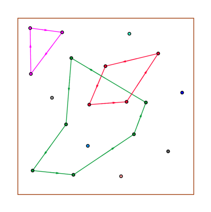
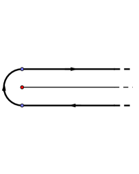
where is the usual (Euclidean) norm in , is the inverse temperature, and a constant term in (1.11) insures the normalization condition (1.10). According to formula (1.9), particles in a random spatial configuration interact with one another via the spatial potential only along cycles of an auxiliary permutation (see Fig. 1), whereby the existence of a cycle of length is either promoted or penalized depending on whether or , respectively.
The link between formulas (1.7) and (1.8) is provided by the function defined by the Fourier transform
| (1.12) |
where denotes the inner product in . For example, the Gaussian potential (1.11) leads to a quadratic function (with ).
From the assumptions on , it readily follows that , (), () and, by the Riemann–Lebesgue lemma, . Since the Fourier transform (1.12) is positive, a simple lemma (see [9, Theorem 9, p. 20] or [18, Lemma 7.2.1, p. 162]) yields that
| (1.13) |
hence the Fourier inversion formula implies the dual relation
Finally, let us assume that the function is regular enough as , so that the integrability condition (1.13) implies the convergence (for any ) of the series
| (1.14) |
For the latter, it is sufficient that, for large enough, is non-decreasing in each of the variables , or that there is a lower bound , with some and . Importantly, the condition (1.14) ensures that the spatial measure (1.7) is well defined.
The model (1.8), (1.9) is motivated by the Feynman–Kac representation of the dilute Bose gas (at least in the Gaussian case), and it has been proposed in connection with the study of the Bose–Einstein condensation (for more details and the background, see [3], [4], [5] and further references therein). An important question in this context, which is also interesting from the combinatorial point of view, is the possible emergence of an infinite cycle under the thermodynamic limit, that is, by letting while keeping constant the particle density . The (expected) fraction of points contained in infinitely long cycles can be defined as
| (1.15) |
Betz and Ueltschi have shown in [6] that in the model (1.7), under certain assumptions on the coefficients , the quantity is identified explicitly as
| (1.16) |
where is the critical density given by
| (1.17) |
That is to say, infinite cycles emerge (in the thermodynamic limit) when the density is greater than the critical density (see further details in [6]).
However, the computations in [6] for the original spatial measure are quite complicated, and it may not be entirely clear as to why the asymptotic behaviour of cycles is drastically different for and (even though intuition does suggest such a phase transition; see a heuristic explanation in [6, p. 1175]).
1.3. Surrogate-spatial model as an approximation of the spatial model
A simple observation that has motivated the present work is that the sum in (1.7) can be viewed, for each fixed , as a Riemann sum (with mesh size ) for the corresponding integral appearing in (1.17). Using Euler–Maclaurin’s (multidimensional) summation formula (see, e.g., [8, § A.4]) and recalling that , this suggests the following plausible approximation of the cycle weights in formula (1.7),
| (1.18) |
with the coefficients
| (1.19) |
(Note that, due to the condition (1.13), the integral in (1.19) is finite for all .) Thus, neglecting the -terms in (1.18), we arrive at the surrogate-spatial model (1.4).
The ansatz (1.18) demands a few comments. In the Gaussian case, with , it can be checked with the help of the Poisson summation formula [10, § 3.12, p. 52] that the expansion (1.18) holds true for any fixed with and (see Section 6.1 below). In general, however, it may not be obvious that the leading correction to the principal term in (1.18) is necessarily constant in .
More importantly, the expansion (1.18) with the integral coefficients (1.19) may fail to be adequate if the index grows fast enough with . For instance, again assuming the Gaussian case, for the sum in (1.18) with we have in dimension
whereas the integral counterpart (see (1.19)) is asymptotic to . This suggests that for close to the relation (1.18) holds with the universal (potential-free) coefficients , . That is to say, the (Gaussian) spatial model dynamically interpolates (up to asymptotically small correction terms) between the surrogate-spatial model with , (for small ) and the one with , (for large ).
We postpone a detailed comparison of the models (1.5) and (1.7) until Section 6. For now let us just point out that both models, after a suitable calibration, share the same critical density and the expected fraction of points in infinite cycles (see (1.17)); there are also qualitative similarities in the transition from the Poisson–Dirichlet distribution of large cycles to a single giant cycle (see Section 5).
1.4. Synopsis and layout
As will be demonstrated in this paper, the class of surrogate-spatial measures defined by (1.5) produces a rich picture of the asymptotic statistics of permutation cycles as , being at the same time reasonably tractable analytically. Thus, despite lacking direct physical relevance, it can be used as an efficient exploratory tool in the analysis of more complicated spatial models.
More specifically, the asymptotics of the surrogate-spatial model can be characterized using the singularity analysis of the generating functions of the sequences and ,
| (1.20) |
In particular, the emergence of criticality is determined by the condition , where is the radius of convergence of the power series ; this inequality defines the supercritical regime, with the subcritical counterpart represented by the opposite inequality, . In the limit , the criticality is manifested as a phase transition in the cycle statistics when the system passes through the critical point.
Remark 1.1.
The phase transition can be parameterized by scaling the coefficients (). Then the critical value of the parameter is given by , with the subcritical and supercritical domains corresponding to the intervals and , respectively. We will argue in Section 6.2 below that the scaling parameter can be viewed as an analogue of the particle density (cf. (1.19)).
Remark 1.2.
We will routinely assume that is analytic in the disk , which allows us to distill the role of the leading sequence in the surrogate-spatial model (1.4). However, will be permitted to have a singularity at (usually of a logarithmic type), which may have significant impact on the asymptotic statistics of long cycles (see Section 5).
The first evidence of the different asymptotic statistics of cycles in the subcritical vs. supercritical regimes is provided by the (weak) law of large numbers for individual cycle counts, as , where is the (unique) root of the equation if and otherwise (see Theorem 4.1).
This result is heuristically matched by the law of large numbers for the total number of cycles , stating that . In all cases, fluctuations of appear to be of order of , and a central limit theorem holds in both subcritical and supercritical regimes (Theorem 4.4 (a), (b)). The critical case can be studied as well (see Theorem 4.4 (c)), but the situation there is more complicated, being controlled by the analytic structure of the generating functions and at the singularity point ; in particular, if has a non-degenerate logarithmic singularity (e.g., with , which corresponds to a geometric sequence ), then it is possible that the limiting distribution of includes an independent gamma-distributed correction to a Gaussian component (see Theorem 4.4 (c-iii)).
The criticality is further manifested by a phase transition in the fraction of points contained in long cycles (cf. (1.15)); namely, we will see (Theorems 4.2 and 4.3) that such a fraction is asymptotically given by and so is strictly positive in the supercritical regime. The quantity can also be interpreted (see Theorem 4.6) as the full mass of the limiting distribution of individual cycle lengths (under a convenient ordering called lexicographic).
The statistics of long cycles emerging in the supercritical regime will be investigated in Section 5. Our main result there is Theorem 5.9 stating that if the generating function has a logarithmic singularity at with (cf. above), then the cycle lengths, arranged in decreasing order and normalized by , converge to the Poisson–Dirichlet distribution with parameter . Furthermore, if then the limiting distribution of the cycle order statistics is reduced to the deterministic vector , meaning that there is a single giant cycle of length (see Theorem 5.13).
The rest of the paper is organized as follows. Section 2 contains the necessary preliminaries concerning certain generating functions, including a basic identity deriving from Pólya’s Enumeration Theorem (see Lemma 2.2). In Section 3, with the help of complex analysis we prove some basic theorems enabling us to compute the asymptotics of (the coefficients of) the corresponding generating functions. In Section 4, we apply these techniques to study the cycle counts, the total number of cycles and also the asymptotics of lexicographically ordered cycles. In Section 5, we study the asymptotic statistics of long cycles. Finally, we compare our surrogate-spatial model with the original spatial model in Section 6.
2. Preliminaries
2.1. Generating functions
We use the standard notation and for the sets of integer and natural numbers, respectively, and also denote .
For a sequence of complex numbers , its (ordinary) generating function is defined as the (formal) power series
| (2.1) |
As usual [15, § I.1, p. 19], we define the extraction symbol , that is the coefficient of in the power series expansion (2.1) of .
The following simple lemma known as Pringsheim’s Theorem (see, e.g., [15, Theorem IV.6, p. 240]) is important in the singularity analysis of asymptotic enumeration problems, where generating functions with non-negative coefficients are usually involved.
Lemma 2.1.
Assume that for all , and let the series expansion (2.1) have a finite radius of convergence . Then the point is a singularity of the function .
The generating functions with the coefficients (cf. and introduced in (1.20)) are instrumental in the context of permutation cycles due to the following important result. Recall that the cycle counts are defined as the number of cycles of length in the cycle decomposition of permutation (see the Introduction). The next well-known identity is a special case of the general Pólya’s Enumeration Theorem [29, § 16, p. 17]; we give its proof for the reader’s convenience (cf., e.g., [24, p. 5]).
Lemma 2.2.
Let be a sequence of (real or complex) numbers. Then there is the following (formal) power series expansion
| (2.2) |
where are the cycle counts. If either of the series in (2.2) is absolutely convergent then so is the other one.
Proof.
Dividing all permutations into classes with the same cycle type , that is, such that (), we have
| (2.3) |
where means summation over non-negative integer arrays satisfying the condition (see (1.1)), and denotes the number of permutations with cycle type .
Furthermore, allocating the elements to form a given cycle type ) and taking into account that (i) each cycle is invariant under cyclic rotations (thus reducing the initial number of possible allocations by a factor of ), and (ii) cycles of the same length can be permuted among themselves (which leads to a further reduction by a factor of ), it is easy to obtain Cauchy’s formula (see, e.g., [1, § 1.1])
| (2.4) |
Hence, using (2.3) and (2.4) and noting that , the right-hand side of (2.2) is rewritten as
which coincides with the left-hand side of (2.2).
The second claim of the lemma follows by the dominated convergence theorem. ∎
Lemma 2.2 can be used to obtain a convenient expression for the normalization constant involved in the definition of the surrogate-spatial measure (see (1.5), (1.6)). More generally, set and
| (2.5) |
In particular (see (1.6)) we have . By Lemma 2.2 (with ), it is immediately seen that the generating function of the sequence is given by
| (2.6) |
where we define the function
| (2.7) |
with the generating functions and defined in (1.20). Hence, the coefficients can be represented as
| (2.8) |
In particular, for formula (2.8) specializes to
| (2.9) |
2.2. Some simple properties of the cycle distribution
In what follows, we use the Pochhammer symbol for the falling factorials,
| (2.10) |
Denote by the expectation with respect to the measure (see (1.5)).
Lemma 2.3.
For each and any integers , we have
| (2.11) |
where and .
Proof.
Next, let be the total number of cycles,
| (2.13) |
Lemma 2.4.
For each , the probability generating function of is given by
| (2.14) |
where the expansion of the function on the right-hand side of (2.14) is understood as a formal power series.
Proof.
One convenient way to list the cycles (and their lengths) is via the lexicographic ordering, that is, by tagging them with a suitable increasing subsequence of elements starting from .
Definition 2.1.
For permutation decomposed as a product of cycles, let be the length of the cycle containing element , the length of the cycle containing the smallest element not in the previous cycle, etc. The sequence is said to be lexicographically ordered.
It is easy to compute the joint (finite-dimensional) distribution of the lengths .
Lemma 2.5.
For each and any (with ), we have
| (2.15) |
In particular, for
| (2.16) |
Proof.
Note that there are cycles of length containing the element , and the choice of such a cycle does not influence the cycle lengths of the remaining cycles. Using the definition (2.5) of we get
which proves the lemma for (see (2.16)). Similarly, for
| (2.17) |
(cf. (2.15)). The general case is handled in the same manner. ∎
3. Asymptotic Theorems for the Generating Function
In this section, we develop complex-analytic tools for computing the asymptotics of the coefficient in the power series expansion of (see (2.8)). More generally, it is useful to consider expansions of the function , with some parameter . From Lemma 2.3 it is clear that the case is of primary importance, but Lemma 2.4 suggests that information for will also be needed for the sake of limit theorems for cycles (see Sections 4 and 5). General considerations in Sections 3.1 – 3.4 below are illustrated by a few important examples (Section 3.5).
3.1. Preliminaries and motivation
Let us introduce notation for the “modified” derivatives of a function ,
| (3.1) |
For the generating functions , (see (1.20)) it is easy to see that, for each ,
| (3.2) |
where is the Pochhammer symbol defined in (2.10).
Let (possibly ) be the radius of convergence of the power series , and hence of each of its (modified) derivatives . If then, according to Pringsheim’s Theorem (see Lemma 2.1), is a point of singularity of (and each , see (3.2)). We write , with if this limit is divergent. For , let us also denote
| (3.3) |
The following simple lemma will be useful.
Lemma 3.1.
For any ,
| (3.4) |
where the inequality is in fact strict unless for all .
Proof.
To avoid trivial complications (or simplifications), let us impose
Assumption 3.1.
The sequence is assumed to be non-arithmetic, that is, there is no integer such that the inequality would imply that is a multiple of . We also suppose that is non-degenerate, in that for some .
Remark 3.1.
The assumption of non-arithmeticity simplifies the analysis by ensuring there is a unique maximum of (the real part of) the generating function (see Lemma 3.2 below). However, a more general case (with multiple maxima) can be treated as well, without too much difficulty. Note also that in the original spatial model (see (1.18), (1.19)) all coefficients are positive, hence such a sequence is automatically non-arithmetic.
In what follows, denotes the real part of a complex number , and is the principal value of its argument.
Lemma 3.2.
(a) Under Assumption 3.1, for each there is a unique maximum of the function over , attained at and equal to . If then this claim is also true with .
(b) The same statements hold for the function , .
Proof.
(a) Since the coefficients are non-negative, is always a point of global maximum of the function . It is easy to see that the uniqueness of this maximum over is equivalent to the property that cannot be written as with a holomorphic function and some integer , and the latter is true because the sequence is non-arithmetic due to Assumption 3.1.
(b) The same considerations are valid for the function which is again a power series with non-negative non-arithmetic coefficients. ∎
Remark 3.2.
The uniqueness part of Lemma 3.2 (b) may fail for with , because the non-arithmeticity property may cease to hold, like in the following example: , , ().
Remark 3.3.
Setting with , , let us consider the Taylor expansion of near with respect to ,
| (3.5) |
where , are defined in (3.3). Note that and the function is real analytic and strictly increasing for (of course, provided that is not identically zero). Thus, the inverse of exists for . For , let be the (unique) solution of the equation
| (3.6) |
In particular, for we have .
Definition 3.2.
The cases and are termed “subcritical” and “supercritical”, respectively.
This terminology will be justified in Section 4 below, in particular by Theorem 4.2, where we will demonstrate that the limiting fraction of points in infinite cycles is positive if and only if . In Section 6, it will also be shown that the dichotomy in Definition 3.2 corresponds to the cases and , respectively, with standing for the system “density” (see Section 6.2 below).
The analytical reason for such a distinction becomes clear from the following observation. Proceeding from the expression (2.9) for , with the function defined in (2.7), Cauchy’s integral formula with the contour () gives
| (3.7) |
Hence, the classical saddle point method (see, e.g., [10, Ch. 5]) suggests that the asymptotics of the integral (3.7) are determined by the maximum of the function . In turn, by Lemma 3.2 (a) this is reduced to finding the maximum of the function for real , leading to the equation
which, in view of Lemma 3.2 (b), is solvable if and only if .
3.2. The subcritical case
In what follows, we shall frequently use a standard shorthand for , or equivalently . The same symbol will have a similar meaning for other limits (e.g., as ).
Theorem 3.3.
Proof.
First of all, according to (2.9) formula (3.9) readily follows from (3.8) by setting and , whereby . To handle the general case, apply Cauchy’s integral formula with the contour to obtain
| (3.10) |
where , and are the corresponding integrals arising upon splitting the interval into three parts, with . Choosing with and small enough, we estimate each of the integrals in (3.10) as follows.
(i) By Taylor’s expansion (3.5) at , with (see (3.3), (3.6)), we have
| (3.11) |
On the change of variables , the integral in (3.11) becomes
as long as . Hence, returning to (3.11) we get
| (3.12) |
3.3. The supercritical case
3.3.1. The domain
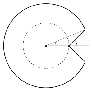
Recall (see Definition 3.2) that the supercritical case occurs when , whereby the equation is no longer solvable. To overcome this difficulty, we have to allow the contour of integration in Cauchy’s integral formula akin to (3.7) to go outside the disk of convergence . To make this idea more precise, we give the following definition (see Fig. 2).
Definition 3.3.
For and , define an open domain in the complex plane by
We also introduce the notation for the radius of the outer circle, , and the angle , so that .
Lemma 3.4.
Suppose that Assumption 3.1 holds, and let be holomorphic in a domain as defined above, with . Then there exist constants , such that, for all with , ,
| (3.15) |
Proof.
By Lemma 3.2 (b), if and then
| (3.16) |
Along with , the function is also analytic in , and in particular it is continuous in a vicinity of the punctured circle . Hence, by a compactness argument the inequality (3.16) also holds on a closed domain
with small enough. Moreover, by the continuity of the strict inequality (3.16) implies that
Therefore, for any we have
| (3.17) |
On the other hand,
| (3.18) |
Hence, combining (3.17) and (3.18) we obtain
and the inequality (3.15) readily follows in view of Lemma 3.2 (a). ∎
Motivated by the model choice (see Section 3.5.2 below), in the supercritical asymptotic theorems that follow we allow the generating function to have a logarithmic singularity at , of the form as (). It turns out that there is a significant distinction between the cases and .
3.3.2. Case
We first handle the case with a non-degenerate log-singularity of .
Theorem 3.5.
Let the generating functions and both have radius of convergence and be holomorphic in some domain as in Definition 3.3. Assume that and the following asymptotic formulas hold as (), with some , ,
| (3.19) | ||||
| (3.20) |
Finally, let be a holomorphic function such that for some
| (3.21) |
Then, provided that , we have, as ,
| (3.22) |
uniformly in for any . In particular, for
| (3.23) |
Proof.
In view of the identity (2.9), formula (3.23) is obtained from (3.22) by setting (so that ) and . Let us also observe that, according to (3.19) and (3.21),
Thus, accounting for the pre-exponential factor just leads to the change . With this in mind, it suffices to consider the basic case (but now with ).
Without loss of generality, we may and will assume (by slightly reducing the original domain if necessary) that both and are continuous on the boundary of except at . By virtue of Lemma 3.4 (and again reducing as appropriate), we may also assume that the inequality (3.15) is fulfilled for all such that and , with some , where (see Definition 3.3).
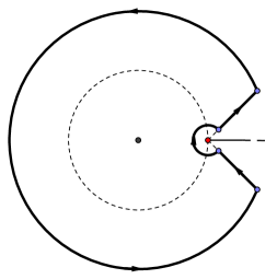
Consider a continuous closed contour (see Fig. 3(a)), where
| (3.24) | ||||
According to the chosen parameterization in (3.24), the contour is traversed anti-clockwise. Then Cauchy’s integral formula yields
| (3.25) |
Now, we estimate each of the integrals in (3.25). Denote for short
| (3.26) |
(i) Let us first show that the integral over the circular arc (see (3.24)) is negligible as . Indeed, by an absolute value inequality we have
| (3.27) |
where and, by Lemma 3.4,
| (3.28) |
Hence, the right-hand side of the bound (3.27) is further estimated by
| (3.29) |
(see the notation (3.26)), which is exponentially small as compared to the right-hand side of (3.22), thanks to the inequalities and . Thus,
| (3.30) |
(ii) For (see (3.24)), we have
| (3.31) |
Then formulas (3.19) and (3.20) yield the uniform asymptotics, as ,
| (3.32) | ||||
| (3.33) |
We also have
| (3.34) |
Collecting (3.32), (3.33) and (3.34), we obtain from (3.25) via the change of variables (3.31)
| (3.35) |
(iii) By the symmetry between the contours and , it is easy to see that the corresponding integrals and are complex conjugate to one another. Hence, it suffices to consider, say, . Similarly to (3.31), we reparameterize the contour (see (3.24)) as
| (3.36) |
Let us split the contour into three parts corresponding to , with , as , and denote the respective parts of the integral by , and . Because the substitutions (3.31) and (3.36) are formally identical to one another, it is clear that the estimates (3.32), (3.33) and (3.34) hold true for (3.36) and, moreover, are uniform in such that , with small enough. Hence, the asymptotics of the integral is given by a formula analogous to (3.35),
| (3.37) |
where (cf. (3.36))
| (3.38) |
Similarly, the integral is asymptotically estimated as
| (3.39) |
provided that and (see (3.26)).
By the continuity of , for in (3.36) with there is a uniform bound
| (3.40) |
On the other hand, the estimate (3.15) of Lemma 3.4 takes the form
| (3.41) |
whereby
| (3.42) |
Hence, using (3.34) and (3.40) – (3.42) we can adapt the estimation in (3.39) to obtain
| (3.43) |
because and (see (3.26)).
Finally, collecting the contributions from (see (3.30), (3.35) and (3.44)) and returning to (3.25) yields, upon the change of the integration variable ,
| (3.45) |
with , where is defined via (3.31) and (3.38) (see Fig. 3(b)).
The integral on the right-hand side of (3.45) can be explicitly computed. Indeed, by virtue of a simple estimate
one can apply a standard contour transformation argument to replace the contour in (3.45) by the “loop” contour starting from , winding clockwise about the origin and proceeding towards (see Fig. 3(c)), which leads to the equality
| (3.46) |
according to the well-known Hankel’s loop representation of the reciprocal gamma function (see, e.g., [15, § B.3, Theorem B.1, p. 745]). This completes the proof of Theorem 3.5. ∎
3.3.3. Case
Note that the deceptively simple case (leading to in (3.19)) is not covered by Theorem 3.5, unless . The reason is that, in the lack of a logarithmic singularity of at , the main term in the asymptotic formula (3.22) vanishes (as suggested by the formal equality ). Thus, in the case the singularity of at should become more prominent in the asymptotics. The full analysis of the competing contributions from the singularities of and can be complicated (however, see Remark 3.4 below), so for simplicity let us focus on the role of assuming that is regular (e.g., ).
Theorem 3.6.
Let the generating function have radius of convergence and be holomorphic in a domain as in Definition 3.3. Assume that and, furthermore, there is a non-integer such that for all while for , and the following asymptotic expansion holds as (),
| (3.47) |
with some , . As for the generating function , it is assumed to be holomorphic in the domain and, moreover, regular at point . Finally, let be a holomorphic function such that, with some and , as (),
| (3.48) |
Then, depending on the relationship between and , the following asymptotics hold as , uniformly in for any .
(i) If then
| (3.49) |
(ii) If is non-integer and then
| (3.50) |
(iii) If then
| (3.51) |
In particular,
| (3.52) |
Proof.
The proof proceeds along the lines of the proof of Theorem 3.5, with suitable modifications indicated below. In what follows, we may and will assume that .
Under the change of variables , with (see (3.31)), by virtue of the expansions (3.47), (3.48) and the regularity of we obtain the uniform asymptotics (cf. (3.32), (3.33))
| (3.53) | ||||
| (3.54) | ||||
with . We can also write (cf. (3.34))
Substituting these expansions into the integral over the contour (see (3.25)), we obtain similarly to (3.35)
| (3.55) |
where (see (3.26)) and , are polynomials in ,
Noting that uniformly in , we can Taylor expand the exponential under the integral in (3.55) keeping the terms up to the order . Thus, we obtain
where is the resulting polynomial in .
A similar estimation holds for the integral (cf. (3.44)). As a result, we get (cf. (3.45))
| (3.56) |
Since is an entire function of , its contribution to the integral (3.56) vanishes,
| (3.57) |
Furthermore, changing the integration variable and transforming the contour to the loop contour (see before equation (3.46)), we obtain
| (3.58) |
according to Hankel’s identity akin to (3.46) (see [15, § B.3, Theorem B.1, p. 745]). As for the term in (3.56), if then its contribution also vanishes (cf. (3.57)), but if is non-integer then, similarly to (3.58), we have
| (3.59) |
It remains to note that the contributions (3.58) and (3.59) enter the asymptotic formula (3.56) with the weights and , respectively, so the relationship between the exponents and determines which of these two terms is the principal one in the limit as . Accordingly, retaining one of the power terms in (3.56) (or both, if ) and dividing everything by (cf. (3.25)) , we arrive at formulas (3.49), (3.50) and (3.51), respectively.
Remark 3.4.
Analogous considerations as in the proof of Theorem 3.6 can be used to handle the case with a power-logarithmic term () added to the expansion (3.47) of , where the index is now allowed to be integer; this is motivated by the choice with , leading to the polylogarithm with the asymptotics (3.115) (see Section 3.5.2 below). Furthermore, the condition of regularity of at imposed in Theorem 3.6 is also not essential, and may be extended to include a power singularity of the form (with and some non-integer ) and, possibly, a power-logarithmic singularity, similarly to what was said above about (with any ). We leave the details to the interested reader.
3.4. The critical case
3.4.1. First theorems
Here , and the equation is still solvable for all , with the unique root (see (3.6)). Thus, the same argumentation may be applied as in the proof of Theorem 3.3, but for this to cover the case one has to assume that , because the circle to be used in Cauchy’s integral formula passes through the singularity if (with ). Recall that the function is defined in (2.6), and is given by (3.3).
Theorem 3.7.
Assume that both and have radius of convergence , with , and, moreover, , . Let be a function holomorphic in the open disk and continuous up to the boundary . Then, uniformly in with an arbitrary constant , we have
| (3.60) |
In particular,
| (3.61) |
Proof.
Note that Taylor’s expansion (3.5) extends to , with , (see (3.3)). Then, on account of the continuity of and on each circle , it is easy to check that the proof of Theorem 3.3 is valid with any , thus leading to (3.60) (cf. (3.8)). As before, formula (3.61) follows from (3.60) by setting and , making . ∎
If has a logarithmic singularity at , we can still use the same argumentation as in Theorem 3.5 as long as .
Theorem 3.8.
Assume that and both have radius of convergence and are holomorphic in some domain as in Definition 3.3. Let , , and suppose that for some , , as (),
| (3.62) | ||||
| (3.63) |
Finally, let be a holomorphic function such that for some
Then, as ,
(a) uniformly in with arbitrary ,
| (3.64) |
(b) uniformly in with arbitrary , provided that ,
| (3.65) |
Proof.
Note that, unlike Theorem 3.7, both parts (a) and (b) of Theorem 3.8 do not cover the value and so do not provide the asymptotics of . Moreover, the asymptotic expressions on the right-hand side of (3.64) and (3.65) vanish as , which suggests that no uniform statements are possible on intervals (even one-sided) that contain the point . Nevertheless, the case can be handled by a more careful adaptation of the proof of Theorem 3.5. First, we need to compute some complex integrals emerging in the asymptotics.
3.4.2. Two auxiliary integrals
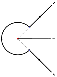
Let be a continuous contour composed of the parts defined as follows (see Fig. 3(b)),
| (3.66) | ||||
with and . For any real parameter , let us consider the contour integral
| (3.67) |
The determination of in (3.67) is defined by the principal branch when is negative real, and then extended uniquely by continuity along the contour. An absolute value estimate gives for
| (3.68) |
where according to the chosen range of . Hence, the integral (3.67) is absolutely convergent for all complex and, moreover, the function is holomorphic in the entire complex plane . An explicit analytic continuation from the domain is furnished through the following functional equation (which can be easily obtained from (3.67) by integration by parts),
From the estimate (3.68) it also follows that the integral (3.67) does not depend on the choice of the angle and the arc radius ; in the computation below, we will choose and take the limit .
It is straightforward to calculate a few values of , such as
A general formula for the integral (3.67) is established in the next lemma.
Lemma 3.9.
For any and all , there is the identity
| (3.69) |
In particular, for we have
| (3.70) |
Proof.
It suffices to prove (3.69) for real (an extension to arbitrary will follow by analytic continuation). As already mentioned, we can choose in (3.66), so that the parts of the original contour take the form
| (3.71) | ||||
Here the parameter is arbitrary, and the idea is to send it to zero.
First of all, since we have assumed that , the integral over vanishes as . Next, using the parameterization (3.71) of the contour we compute
| (3.72) |
A similar computation for gives
| (3.73) |
Combining (3.72) and (3.73), by using Euler’s formula and some elementary trigonometric identities we obtain
| (3.74) |
where
| (3.75) |
For the integrals (3.75) are given by (see [16, # 3.952 (7, 8), p. 503])
| (3.76) | ||||
| (3.77) |
where is the confluent hypergeometric function (see [16, # 9.210 (1), p. 1023]),
| (3.78) |
with . It is easy to see (e.g., using the ratio test) that the series (3.78) converges for all , and hence is an entire function of . In particular, .
Substituting the expressions (3.76), (3.77) into (3.74) and using (twice) the well-known complement formula for the gamma function (see, e.g., [15, § B.3, pp. 745–746])
| (3.79) |
we obtain
| (3.80) |
Furthermore, observe from (3.78) that
| (3.81) |
and similarly
| (3.82) |
Now, returning to (3.80) and combining the sums in (3.81) and (3.82) we arrive at (3.69).
There is a simple probabilistic representation of the power series part of the expression (3.69), which will be helpful in applications (see the proof of Theorem 4.4 (c-iii) below).
Lemma 3.10.
Let be a random variable with gamma distribution (), that is, with probability density , . Then the moment generating function of is given by
| (3.83) |
Proof.
A similar argumentation as in Lemma 3.9 may be applied to the integral
| (3.85) |
with the contour as defined in (3.66). Note that for the integral (3.85) is reduced to (3.70): . The general case is handled in the next lemma.
Lemma 3.11.
For any , the following identity holds
| (3.86) |
Proof.
Like in the proof of Lemma 3.9, it suffices to consider the case . Then, similarly to (3.72) and (3.73), we obtain (cf. (3.74))
| (3.87) |
Note that, according to the condition , we have . By the change of variable and with the help of some standard trigonometric identities, the integral on the right-hand side of (3.87) is rewritten as
| (3.88) |
where
These integrals can be explicitly computed as follows (see [16, # 3.944 (5, 6), p. 498])
where
Substituting this into (3.87) and (3.88) we get
again using the complement formula (3.79). Hence, the result (3.86) follows. ∎
3.4.3. Asymptotic theorems with
We are now in a position to obtain “dynamic” asymptotic results for the critical case in the neighbourhood of . For simplicity, we omit the pre-exponential factor (which will not be needed). First, let us consider a “regular” case where the second derivative of at is finite.
Theorem 3.12.
Proof.
Setting , we adapt the proof of Theorem 3.5 by making the following modifications:
Note that due to the criticality assumption, the quantity (see (3.26)) is reduced to zero for , so that the estimate (3.29) of the asymptotic contribution of the integral becomes void. This can be fixed by taking advantage of an enhanced version of the inequality (3.28) provided by Lemma 3.4 (see (3.15)), leading to an improved bound
Next, under the substitution , using (3.63) and the expansion
we have, as ,
| (3.91) |
Combined with the expansion (cf. (3.34))
| (3.92) |
this leads to the following asymptotics of the integral as (cf. (3.35))
| (3.93) |
where and .
The integral is asymptotically evaluated in a similar fashion (cf. (3.44)), leading to the same formula as (3.93) but with the contour of integration defined in (3.38). Note that the error terms (3.39) and (3.43), formally invalidated by , can be adapted by using Lemma 3.4 as described above.
As a result, collecting the principal asymptotic terms from formula (3.93) and its other counterparts (cf. (3.37)) produces the integral , according to the notation (3.67). Hence, we arrive at the expression (3.89), as claimed. Finally, (3.90) immediately follows from (3.89) by setting and on using formula (3.70). ∎
Remark 3.5.
Let us now study the case with an infinite second derivative of at .
Theorem 3.13.
Proof.
In what follows, we can assume that . Again setting , we adapt the proof of Theorem 3.12 by using the change of variables . Hence, the expansions (3.91) and (3.92) are replaced, respectively, by
and
Similarly as in the proof of Theorem 3.13, this leads to the asymptotics (cf. (3.93))
with the rescaled contour . The integral is estimated similarly (cf. (3.44)). As a result, recalling the notation (3.85) we obtain
3.5. Examples
Let us give a few simple examples to illustrate the conditions of the asymptotic theorems proved in Sections 3.2 – 3.4.
3.5.1. Constant coefficients
For all , let , . Then the corresponding generating functions specialize to
| (3.96) |
Recalling the expression (2.8) and using the binomial series expansion, we have explicitly
| (3.97) |
and with Stirling’s formula for the gamma function this yields, for any ,
| (3.98) |
To apply the general machinery developed in Section 3.2, from (3.96) we find
| (3.99) |
so that the expressions (3.3) specialize to
| (3.100) |
Here and , , so that, according to our terminological convention in Section 3.1 (see Definition 3.2), we are always in the subcritical regime. In view of (3.99), the solution of the equation (3.6) is explicitly given by
| (3.101) |
Setting , from (3.96), (3.100) and (3.101) we find
and Theorem 3.3 (with and readily yields the same result as (3.98).
Remark 3.6.
In the degenerate case with , (which is nothing more than the Ewens model), a direct calculation using (3.97) gives
| (3.102) |
3.5.2. Polylogarithm
To illustrate the supercritical and critical regimes, we need examples with . To this end, let us set () with , , so that the corresponding generating function is proportional to the polylogarithm (see, e.g., [23])
| (3.103) |
For the model (3.103) is reduced to the case considered in Section 3.5.1. Clearly, has the radius of convergence for any , and for , where is the Riemann zeta function. Differentiating (3.103) we get
| (3.104) |
and so the supercriticality condition reads
| (3.105) |
Similarly,
| (3.106) |
and so
Hence, substituting (3.104) and (3.106) into (3.3) we obtain
Furthermore, from (3.104) we find that the root of the equation (3.6) is given by
| (3.107) |
where is the inverse of . Differentiating the identity (3.107) we also obtain
In particular,
The supercritical case is more interesting. It is known (see, e.g., [15, § IV.9, p. 237, and § VI.8, p. 408] that the polylogarithm can be analytically continued to the complex plane slit along the ray . The asymptotic behaviour of near is specified as follows (see [15, Theorem VI.7, p. 408, and § VI.20, p. 411]).
Lemma 3.14.
With the notation
| (3.108) |
the polylogarithm satisfies the following asymptotic expansion as :
(a) if then
| (3.109) |
(b) if then
| (3.110) |
where (with ).
Remark 3.7.
The restriction in the sum (3.110) respects the fact that the zeta function has a pole at .
Remark 3.8.
In the simplest case the expansion (3.110) specializes to
which should be contrasted with the explicit expression (). Of course, there is no contradiction; the corresponding identity
| (3.111) |
with the left-hand side defined at by continuity as , can be verified using that , for odd and for even (see, e.g., [15, § B 11, p. 747]), where are the Bernoulli numbers (see, e.g., [15, p. 268]) defined by the generating function (note that , and for odd ). Indeed, (3.111) is then rewritten as
and the proof is completed by differentiation of both sides with respect to .
Explicit asymptotic expansion of in terms of , to any required order, can be obtained by substituting the series (3.108) into (3.109) or (3.110) as appropriate. In particular, for the generating function of the form (3.103) with (), from formulas (3.108) and (3.109) we get the Taylor-type expansion
| (3.112) |
where the coefficients
are expressible as linear combinations of the zeta functions (),
Furthermore, using similar arguments it is easy to see that the expansion (3.112) can be differentiated any number of times, yielding the asymptotics
| (3.113) | |||||
| (3.114) |
By virtue of formula (3.112), and by choosing suitable (non-integer) values of the parameter in (3.103), one can easily construct examples matching the assumptions of each of the asymptotic theorems in Sections 3.3 and 3.4. Moreover, the asymptotic formulas (3.113) and (3.114) make the polylogarithm example (3.103) suitable for the setting of Section 5 below (see the assumptions (5.1), (5.2)).
The case with integer leads to a logarithmic term in the singular part of the asymptotic expansion at . Indeed, if then formula (3.103) is reduced to
while corresponds to , so that using (3.108) and (3.110) one obtains with an arbitrary (cf. (3.112))
| (3.115) |
where is the coefficient of the term arising from the expansion (3.110) (with replaced by ) upon the substitution (3.108).
3.5.3. Perturbed polylogarithm
A natural extension of the polylogarithm example considered in the previous subsection is furnished by setting (), where , , for all , and the perturbation function is assumed to be analytic in the half-plane and to satisfy there the estimate , with some . It follows that the corresponding generating function
| (3.116) |
is analytic in the disk , with singularity at . Furthermore (see (3.104)),
| (3.117) |
As suggested by the principal term in (3.117), the criticality occurs if (cf. (3.105)); indeed, with a suitable constant we have for sufficiently small
| (3.118) |
Lemma 3.15.
Under the above conditions on (with ), the function can be analytically continued to the slit complex plane .
Proof.
Since the claim is valid for the polylogarithm (see Section 3.5.2), from (3.116) we see that it suffices to prove the lemma for the series , where . Clearly, for any we have the estimate . Hence, the Lindelöf theorem (see [15, § IV.8, p. 237] yields the integral representation
| (3.119) |
which provides an analytic continuation of the series to the domain . Since can be taken arbitrarily small, this implies the analyticity in slit along the ray . To complete the proof, it remains to recall that is analytic in . ∎
The next question is the asymptotic behaviour of the function (3.116) as with . Application of the asymptotic formulas (3.109) and (3.110) in the particular case (leading to ) motivates and illustrates the following expansions, which now have to be finite (up to the order of ) due to the limited information about the perturbation function .
Lemma 3.16.
Suppose that satisfies the same conditions as in Lemma 3.15, and let be such that . Then, as so that ,
(a) for (i.e., ),
| (3.120) |
where if , if , and is any number in if ;
(b) for ,
| (3.121) |
where is some constant, if and is any number in if .
Sketch of proof.
This result is of marginal significance for our purposes, as it will only be used for illustration in Section 6.3. Its full proof is quite tedious but follows very closely the proof of a similar result for the polylogarithm (see details in [15, § VI.8]). Thus, we opt to derive the expansion (3.120) only for real ; an extension to complex is based on the Lindelöf integral representation (3.119).
Observe that it suffices to prove (3.120) for ; the case of an arbitrary (non-integer) may then be handled via a suitable (-fold) integration over the interval . To this end, using the substitution (with as ), from (3.116) we obtain
| (3.122) |
The first series in (3.122) may be rewritten as a Riemann integral sum
| (3.123) |
where the asymptotics on the right-hand side can be obtained using Euler–Maclaurin’s summation formula. The integral in (3.123) is easily computed via integration by parts,
| (3.124) |
Next, using the estimate and assuming that , the second series in (3.122) is estimated, similarly to (3.123) and (3.124), by
| (3.125) |
4. Asymptotic Statistics of Cycles
Throughout this section, we assume that the generating functions and satisfy the hypotheses of a suitable asymptotic theorem in Section 3 — namely, Theorem 3.3 for the subcritical case (), Theorems 3.5 or 3.6 for the supercritical case (), and Theorems 3.7, 3.12 or 3.13 for the critical case (.
Remark 4.1.
The analytic conditions on the generating functions and employed in Section 3 are difficult to convert into general sufficient conditions on the underlying coefficients and , respectively. For a better orientation in the asymptotic results below, it should be helpful for the reader to bear in mind the examples (especially the polylogarithm) considered in Section 3.5.
Let us define the quantity as
| (4.1) |
where is the (unique) root of the equation (3.6) with , that is, . Thus, we have
| (4.2) | ||||
4.1. Cycle counts
Our first result treats the asymptotics of the cycle counts (i.e., the numbers of cycles of length , respectively, in a random permutation ).
Theorem 4.1.
Let be as defined in (4.1).
(a) For each and any integers , we have
| (4.3) |
In particular, the random variables are asymptotically independent and, for each , there is the convergence in probability
| (4.4) |
(b) If, for some , but then for any integer
| (4.5) |
Hence, converges weakly to a Poisson law with parameter . The asymptotic independence of with other cycle counts (normalized or not, as appropriate) is preserved.
Remark 4.2.
If both and then, by the definition (1.5) of the measure , almost surely (a.s.).
Proof of Theorem 4.1.
If all then Lemma 2.3 implies that for any
| (4.6) |
where . Furthermore, note that
| (4.7) |
Hence, applying one of Theorems 3.3, 3.5, 3.6, 3.7, 3.12 or 3.13 as appropriate (each one with the pre-exponential function ), we get
| (4.8) |
Combining (4.6) and (4.8) we obtain formula (4.3), which also entails the asymptotic independence. Finally, the convergence (4.4) follows from (4.3) by the method of moments.
Similarly, for , we have
where the limit is the -th factorial moment of the corresponding Poisson distribution. ∎
Remark 4.3.
If for all , then is ill-defined (see (4.1)) and our result does not apply. In this case, it has been proved by Nikeghbali and Zeindler [28, Corollary 3.2] that, under suitable analytic conditions on the generating function in the spirit of those used in Section 3, the cycle counts converge to mutually independent Poisson random variables with parameter , respectively. The latter is easy to see in a simple particular case with (the Ewens model), where by the asymptotics (3.102) and Lemma 2.3
See also Ercolani and Ueltschi [12, Theorem 6.1], where the asymptotically Ewens case has been studied.
Remark 4.4.
Formally, the limiting result (4.4) suggests that the total proportion of points contained in finite cycles, i.e., , is asymptotically given by (see (4.2))
which indicates the emergence of an “infinite” cycle in the supercritical case (i.e., , see Definition 3.2). This observation is elaborated below (see Theorems 4.2 and 4.3).
4.2. Fraction of points in long cycles
By analogy with the spatial case (see (1.15)), let us define the similar quantities in the surrogate-spatial model to capture the expected fraction of points in long cycles,
| (4.9) |
Theorem 4.2.
Proof.
Theorem 4.2 can be complemented by a similar statement about the convergence of the (random) proportion of points in long cycles, rather than its expected value.
Theorem 4.3.
Under the sequence of probability measures , for any finite there is the convergence in probability
| (4.12) |
where is identified in (4.10).
4.3. Total number of cycles
The next result is a series of weak limit theorems (in the subcritical, supercritical and critical cases, respectively) for fluctuations of the total number of cycles (see (2.13)). As stipulated at the beginning of Section 4, we work under the conditions of suitable asymptotic theorems from Section 3, which will be applied without the pre-exponential factor (i.e., with ). Note that in all but one case the limiting distribution is normal, whereas in the critical case with (part (c-iii)) the answer is more complicated (and more interesting).
In what follows, the notation indicates convergence in distribution (with respect to the sequence of measures ), and denotes the standard normal law (i.e., with mean and variance ).
Theorem 4.4.
(a) Let . Then, under the conditions of Theorem 3.3,
| (4.13) |
where is the root of (3.6) with , is defined in (3.3), and .
(c) Let .
(c-ii) Under the conditions of Theorem 3.13,
| (4.15) |
(c-iii) Under the conditions of Theorem 3.12 with ,
| (4.16) |
where is a standard normal random variable and is an independent random variable with gamma distribution .
Proof.
(a) Using Lemma 2.4 and applying Theorem 3.3 (see (3.8)) we obtain as , uniformly in in a neighbourhood of ,
| (4.17) |
where we set for short
| (4.18) |
Using the definition of (see (3.6)), from (4.18) we find
| (4.19) |
Differentiating (4.19) once more gives
| (4.20) |
On the other hand, differentiating the identity (see equation (3.6)), we get
which yields, on account of (3.1) and (3.3),
| (4.21) |
Hence, using (4.19), (4.20) and (4.21) we obtain the expansion of around ,
| (4.22) |
Substituting into (4.22) gives
Besides, for the function from (4.18) we have, for any ,
Therefore, returning to (4.17) we get, as ,
The statement (4.13) now follows by a standard convergence theorem based on convergence of moment generating functions and the well-known fact that if a random variable is standard normal then its moment generating function is given by .
It remains to check that the limit variance is positive. But this follows by Lemma 3.1, yielding
according to the definition of as the root of the equation (3.6) with .
(b) If then, similarly as in (4.17), (4.18), we use Lemma 2.4 and Theorem 3.5 to obtain as , uniformly in in a neighbourhood of ,
Again substituting , the rest of the proof proceeds similarly as in part (a), giving
| (4.23) |
and (4.14) follows.
Likewise, if then by Theorem 3.6 we have from (3.49) and (3.52)
| (4.24) |
and the substitution in (4.24) yields the same asymptotics (4.23).
(c-i) From (3.60), similarly as in part (a), we obtain the asymptotic relation (4.17) that holds uniformly in a right neighbourhood of . The rest of the proof is an exact copy of that in part (a), except that we must use the substitution with .
Remark 4.5.
To summarize the content of Theorem 4.4, the sequence of “phase transitions” manifested by the limit distribution of is as follows. In the subcritical domain (), is asymptotically normal with asymptotic variance (Theorem 4.4 (a)). This is consistent with the critical case () with finite and , whereby (Theorem 4.4 (c-i)). Quite surprisingly, if acquires logarithmic singularity with exponent , the central limit theorem breaks down as the existing normal component of the limit is reduced by the square root of an independent gamma-distributed random variable (Theorem 4.4 (c-iii)). In particular, the limit distribution of gets negatively skewed; for instance, its expected value equals whilst . Thus, although we prove weak convergence using the moment generating functions, the limit in this case cannot be established by the plain method of moments. However, when the function becomes more singular at , with , the limit of reverts to a normal distribution but with a bigger variance, (Theorem 4.4 (c-ii)), which continues to hold in the supercritical regime (Theorem 4.4 (b)).
Despite a complicated structure of the weak limit, the total number of cycles in all cases satisfies the following simple law of large numbers, as .
Corollary 4.5.
Remark 4.6.
4.4. Lexicographic ordering of cycles
We can now find the asymptotic (finite-dimensional) distribution of the cycle lengths (see Definition 2.1). Note that no normalization is needed.
Theorem 4.6.
For each , the random variables are asymptotically independent as and, moreover, for any
| (4.26) |
where is defined in (4.1).
Proof.
Note from (4.26) that the limiting distribution of each has the probability generating function
| (4.27) |
The right-hand side of (4.27) defines a proper probability distribution if (i.e., in the subcritical and critical cases), because then its total mass is given by (see (4.2)). But in the supercritical regime this distribution is deficient, since . Clearly, the reason for this is the emergence of infinite cycles as ; see Theorems 4.2 and 4.3, where the defect is identified precisely as the limiting fraction of points contained in infinite cycles.
However, conditioning on and passing to the limit as gives
which defines a proper distribution.
5. Long Cycles
The ultimate goal of Section 5 is to characterize the supercritical asymptotics of longest cycles (i.e., containing the fraction of points , see Section 4.2). Following the classical approach of Kingman [21] and Vershik and Shmidt [31], we study first the asymptotic extreme value statistics of cycles under lexicographic ordering (see Definition 2.1) and then deduce from this the limit distribution for cycles arranged in the decreasing order of their length.
More specifically, we will show (Theorem 5.6) that if the generating function has a non-vanishing logarithmic singularity at (i.e., with in formula (3.19)), then the lengths of lexicographically ordered cycles normalized by , converge (in the sense of finite-dimensional weak convergence) to the modified GEM distribution with parameter (cf. [1, p. 107]). The latter is constructed via the usual stick-breaking process but applied only to the breakable part of the unit stick , whereas the remaining part causes delays that contribute atoms at zero to the distribution of the output random sequence (see more details in Section 5.3). Using the well-known link between the descending extreme values of the and the Poisson–Dirichlet distribution (see [1, § 5.7]), and noting that delays in the stick-breaking process do not affect the upper order statistics of cycle lengths, Theorem 5.6 will readily imply that the ordered cycle lengths weakly converge to the corresponding Poisson–Dirichlet distribution (Theorem 5.9).
In the case , a similar argumentation works as well (see Theorem 5.12) but here the stick-breaking process of Section 5.3 is reduced to removal of the entire breakable part at first success in a chain of Bernoulli trials with success probability . Translated back to the language of descending order statistics , this means that there is a single giant cycle, with length , emerging in the limit (Theorem 5.13).
Remark 5.1.
Let us point out that although the supercritical regime is defined in terms of the generating function of the sequence , the limit distribution of long cycles (and in particular the distinction between the Poisson–Dirichlet distribution of Theorem 5.9 and the degenerate distribution of Theorem 5.13) is determined entirely by the generating function of the sequence .
5.1. Analytic conditions on the generating functions
For the most part (until Section 5.6), the generating functions and will be assumed to satisfy the hypotheses of Theorem 3.5, including the asymptotic formulas (3.19) and (3.20) (with some ). In particular, so we are in the supercritical regime. Furthermore, let us assume that there is a non-integer such that for all while for ; moreover, there exist a constant and a sequence such that, as , (see Definition 3.3),
| (5.1) | |||||
| (5.2) |
In addition to (3.19), we also assume that
| (5.3) |
In Section 5.6 we will also consider the case , using the results of Theorem 3.6.
5.2. Reminder: Poisson–Dirichlet distribution
Our aim is to show that, under the assumptions stated in Section 5.1 (most importantly, with ), the descending order statistics of the cycle lengths converge to the so-called Poisson–Dirichlet distribution .
Let us recall that the Poisson–Dirichlet distribution with parameter was introduced by Kingman [20, § 5] as the weak limit of order statistics of a symmetric Dirichlet distribution (with parameter ) on -dimensional simplex as , . Such a limit can be identified as the distribution law of the normalized points of a Poisson process on with rate ,
where (a.s.); note that the random variable has the gamma distribution and is independent of the sequence (see, e.g., [22, § 9.3] or [1, § 5.7] for more details).
An explicit formula for the finite-dimensional probability density of , first obtained by Watterson [32, § 2] (see also [1, p. 113]), is quite involved but is of no particular interest to us. There is, however, an equivalent descriptive definition of the Poisson-Dirichlet distribution through the so-called distribution (named after Griffiths, Engen and McCloskey; see, e.g., [1, p. 107]), which is the joint distribution of the random variables
| (5.4) |
where is a sequence of independent identically distributed (i.i.d.) random variables with the beta distribution (i.e., with the probability density , ). From the definition (5.4), it is straightforward to obtain the finite-dimensional probability density of (see [1, p. 107]),
Remark 5.3.
The remarkable link of the with the , discovered by Tavaré [30, Theorems 4 and 6] (see also [1, § 5.7]), is as follows.
Lemma 5.1.
The descending order statistics of the sequence (5.4) have precisely the distribution.
Note that since the joint distribution of ’s is continuous, the order statistics are in fact distinct (a.s.).
5.3. Modified stick-breaking process
Let , be two sequences of i.i.d. random variables each, also independent of one another, where ’s have uniform distribution on and ’s have beta distribution with parameter . Setting , let us define inductively the random variables
| (5.5) |
where () and denotes the indicator of event . Note that ’s are Bernoulli random variables (with values and ), adapted to the filtration and with the conditional distribution
| (5.6) |
where is a trivial -algebra. In particular, , .
Finally, let us consider the random variables
| (5.7) |
Noting that, for all , we have (a.s.), from (5.5) it is clear that
| (5.8) |
which also implies, due to (5.7), that
Remark 5.4.
The random sequence may be interpreted as a modified stick-breaking process with delays (cf. Remark 5.3), whereby the original interval (“stick”) is divided into two parts: (i) which is subject to a subsequent breaking, and (ii) which stays intact. At each step, the breaking is only enabled if an independent point chosen at random in the remaining stick falls in the breakable part, otherwise the process is idle; the breaking, when it occurs, acts as the removal of a fraction of the current breakable part, independently sampled from .
Lemma 5.2.
The random sequence satisfies the a.s.-identities
| (5.9) |
Proof.
Recalling (5.7), we have
| (5.10) |
which proves the first formula in (5.9). To establish the second one, in view of (5.10) we only need to check that a.s. To this end, note that , so that the sequence is non-increasing and therefore converges to a (possibly random) limit . To show that a.s., consider
| (5.11) |
Recalling the definition of (see (5.5)) and noting that and are mutually independent, with also independent of , we obtain, using (5.6) and replacing in the denominator with its upper bound ,
Returning to (5.11) and taking the expectation, we obtain
Passing to the limit as and using the monotone convergence theorem, we deduce that , hence a.s. This completes the proof of the lemma. ∎
Remark 5.5.
In terms of the modified stick-breaking process (see Remark 5.3), the second equality in (5.9) means that, with probability , the total fraction removed from the breakable part of the stick has full measure. This is a generalization of the similar property of the standard stick-breaking process (5.4).
Lemma 5.3.
With probability , infinitely many ’s are non-zero.
Proof.
By Lemma 5.2, (a.s.) as . In view of the last formula in (5.5), this implies that (a.s.), which is equivalent to (a.s.). Hence, infinitely often (a.s.), and the claim of the lemma now readily follows from (5.7) since a.s. (see (5.8)).
The fact that infinitely often (a.s.) can be established more directly as follows. Put and define inductively the successive hitting times
| (5.12) |
with the usual convention . Since (a.s.), from (5.5) we see that (a.s.), while for , so it remains to verify that is an a.s.-infinite sequence. Indeed, from the definition of it follows that
Together with formulas (5.5) and (5.6), this implies that, conditionally on , the random variable is time to first success in a sequence of independent Bernoulli trials with success probability (see (5.6)), so it has the geometric distribution
and in particular a.s. From the product structure of the filtration it is also clear that the waiting times are mutually independent (). Hence, it follows that all are a.s.-finite, as required. ∎
Let be the order statistics built from the sequence (see (5.7)) by arranging the entries in decreasing order. Recall that ; moreover, by Lemma 5.3 infinitely many entries are positive (a.s.) and, in addition, according to Lemma 5.2. It follows that, with probability , there is an infinite sequence of order statistics , each well defined up to possible ties of at most finite multiplicities (however, it will be clear from the next lemma and the continuity of the Poisson–Dirichlet distribution that positive order statistics are in fact a.s.-distinct).
In particular, the sequence is not affected by any zero entries among ’s, which therefore can be removed from prior to ordering. But, according to the definition of the random times (see (5.12)) and by formulas (5.5) and (5.7), successive non-zero entries among are precisely given by
| (5.13) |
where are i.i.d. random variables with beta distribution . The latter claim can be easily verified using the total probability formula and mutual independence of the waiting times pointed out in the alternative proof of Lemma 5.3; for instance,
Lemma 5.4.
The sequence of the descending order statistics has the Poisson–Dirichlet distribution with parameter .
In conclusion of this subsection, let us prove some moment identities for the random variables .
Lemma 5.5.
For each , as ,
| (5.14) |
Furthermore, for all
| (5.15) |
while for and any
| (5.16) |
Proof.
Using the definitions (5.5) and (5.7), we obtain
which proves the first part of formula (5.14). The second part follows by substituting the well-known representation .
To prove (5.15), let us first compute the conditional expectation
| (5.17) |
where, according to (5.5) and (5.6),
Hence, on taking the expectation of (5.17), we obtain
| (5.18) |
For we have , leading to
| (5.19) |
and the substitution of (5.19) into (5.18) gives the first line of formula (5.15). The second line can again be obtained by expressing the beta function through the gamma function.
5.4. Cycles under lexicographic ordering
The next theorem characterizes the asymptotic (finite-dimensional) distributions of normalized cycle lengths under the lexicographic ordering introduced in Definition 2.1. Owing to the normalization proportional to , only long cycles (i.e., of length comparable to ) survive in the limit as . This result should be contrasted with Theorem 4.6 that deals with non-normalized cycle lengths, thus revealing an asymptotic loss of mass in the supercritical regime due to the emergence of long cycles (see a comment after the proof of Theorem 4.6).
Theorem 5.6.
For the proof of the theorem, we first need to establish the following lemma.
Lemma 5.7.
For each ,
| (5.22) |
Furthermore, for any
| (5.23) |
while for and any
| (5.24) |
Remark 5.6.
The subtlety of Lemma 5.7 is hidden in the fact that the asymptotics (5.22), (5.23), (5.24) are invalidated if either of , , takes the value ; for instance, formula (5.24) cannot be readily deduced from (5.23) by setting . An explanation lies in the asymptotic separation of “short” and “long” cycles, leading to the emergence of an atom of mass at zero in the limiting distribution of for .
Proof of Lemma 5.7.
Let us first consider , where is the Pochhammer symbol defined in (2.10). Using the distribution of obtained in Lemma 2.5 (see (2.16)) and recalling formulas (2.8) and (3.2), we get for each
| (5.25) |
In view of the formula (see (4.11)), Theorem 3.5 with function and (see (5.3)) gives
| (5.26) |
Furthermore, using the asymptotic expansions (5.1), (5.2) and applying Theorem 3.5 with and , we obtain
| (5.27) |
due to the conditions , . Thus, substituting (5.26) and (5.27) into (5.25) yields
which implies (5.22).
We now turn to (5.24) and (5.23). Using the joint distribution of and (see (2.15)), it follows by a similar computation as in (5.25) that, for any integers , ,
| (5.28) |
As before, we can work out the asymptotics of (5.28) by using Theorem 3.5 with the function
| (5.29) |
The singularity of each term in (5.29) (and the respective index , see (3.21)) is specified from formulas (5.1), (5.2) and (5.3). First of all, using (5.3) we have
(i.e., ), so formulas (3.22), (3.23) of Theorem 3.5 give
| (5.30) |
which coincides with the asymptotics (5.23).
For , contributions from other terms in (5.29) are negligible as compared to . Indeed, from (5.1) and (5.2) we get
with
thanks to the condition . Hence, by Theorem 3.5 we have
| (5.31) |
Remark 5.7.
As should be clear from the proof, the factor is included in (5.23) and (5.24) in order to cancel the denominator in formula (2.17) of the two-dimensional distribution of . As suggested by the general formula (2.15) of Lemma 2.5, an extension of Lemma 5.7 to the -dimensional case requires the inclusion of the product . The corresponding calculations are tedious but straightforward, and follow the same pattern as for . A suitable extension is also possible for Lemma 5.5.
Proof of Theorem 5.6.
For the sake of clarity, we consider only the case (i.e., involving the joint distribution of ); computations in the general case require an extension of Lemmas 5.5 and 5.7 (see Remark 5.7) and can be carried out along the same lines.
By the continuous mapping theorem and according to the definitions (5.5) and (5.7), the convergence (5.21) with is equivalent to
By the method of moments, it suffices to show that for any , as ,
| (5.34) |
First, for the relation (5.34) is trivial, since both sides are reduced to . If and then (5.34) readily follows from the relations (5.14) (Lemma 5.5) and (5.22) (Lemma 5.7).
To cover the case , let us prove a more general asymptotic relation
| (5.35) |
valid for all and . We argue by induction on . For , the relation (5.35) is verified by comparing formulas (5.15) and (5.23) (for ) or (5.16) and (5.24) (for ). Now suppose that (5.35) is true for some . Expanding
and using the induction hypothesis (5.35), we get
which verifies (5.35) for , and therefore for all . This completes the proof of Theorem 5.6. ∎
5.5. Poisson–Dirichlet distribution for the cycle order statistics
Let us now consider the cycle lengths without the lexicographic ordering, and arrange them in decreasing order.
Definition 5.1.
For a permutation , let be the length of the longest cycle in , the length of the second longest cycle in , etc.
Let us first prove a suitable “cut-off” lemma for lexicographically ordered cycles.
Lemma 5.8.
For any , we have
| (5.36) |
Proof of Lemma 5.8.
Fix a and note that, for all ,
| (5.37) |
Furthermore, noting that
| (5.38) |
by Theorems 4.3 and 5.6 we have, as ,
Returning to (5.38), this gives
Hence, recalling that (see (4.9)), from (5.37) we obtain
Finally, passing here to the limit as and noting that, by Lemma 5.2, (a.s.), we arrive at (5.36), as claimed. ∎
The next theorem is our main result in this subsection. Recall that the parameter is involved in the assumption (5.3).
Theorem 5.9.
In the sense of convergence of finite-dimensional distributions,
where denotes the Poisson–Dirichlet distribution with parameter .
Proof.
By virtue of Lemma 5.4, it suffices to show that, for each ,
| (5.39) |
Let us first verify (5.39) for . Fix an integer and observe that, for any ,
Hence, by Theorem 5.6 and the continuous mapping theorem, it follows that
| (5.40) |
because as . On the other hand, we have an upper bound
and by Theorem 5.6 and Lemma 5.8 this yields (cf. (5.40))
| (5.41) |
Combining (5.40) and (5.41) and assuming that is a point of continuity of the distribution of (which is, in fact, automatically true owing to Lemma 5.4), we obtain
which proves (5.39) with .
The general case is handled in a similar manner, by using lower and upper estimates for the -dimensional probability through the similar probabilities for the order statistics of the truncated sample (), where the “discrepancy” term due to the contribution of the tail part may be shown to be asymptotically negligible as by virtue of the cut-off Lemma 5.8. ∎
Remark 5.8.
As already mentioned in Remark 3.4, the requirement imposed in Section 5.1 that the asymptotic expansion (3.47) of holds with a non-integer index may be extended to allow a power-logarithmic term (with any ). With the asymptotic formulas (5.1), (5.2) modified accordingly, the proof of Lemma 5.7 may be adapted as appropriate, implying that Theorems 5.6 and 5.9 remain true.
5.6. Case
Let us now turn to studying the asymptotic behaviour of cycles in the case (see (3.19)). More precisely, throughout this subsection we suppose that, as in Theorem 3.6, the generating function is holomorphic in a suitable domain (see Definition 3.3) and, moreover, is regular at point ; in particular, the successive (modified) derivatives of have Taylor-type asymptotic expansions, as (),
We also assume that the generating function admits the asymptotic expansion (3.47) of Theorem 3.6 (with a non-integer ), which may be differentiated any number of times to yield a nested family of expansions (with some , ),
| (5.42) |
where the first sum is understood to vanish if (cf. (5.1), (5.2)).
Let us now revisit the modified stick-breaking process underpinning our argumentation in the case in Section 5.3. Observe that if then the beta distribution of the random variables converges to Dirac delta measure , since for any
It is easy to see that, under this limit, equations (5.5) and (5.7) are greatly simplified to the following. Let be a sequence of i.i.d. Bernoulli random variables with success probability . Let (a.s.) be the random time until first success, with geometric distribution
| (5.43) |
Now, for we set
| (5.44) |
Remark 5.9.
The following analogue of Lemma 5.5 is formally obtained by substituting ; its proof is elementary by using the definition (5.44) and the distribution of (see (5.43)).
Lemma 5.10.
For any ,
Next, we prove an analogue of Lemma 5.7, which formally looks as its particular case with (cf. (5.22), (5.23) and (5.24)).
Lemma 5.11.
For any ,
| (5.45) | |||
| (5.46) | |||
| (5.47) |
Proof.
We use similar argumentation as in the proof of Lemma 5.7, but now exploiting Theorem 3.6. First of all, according to (5.25) we have, for any ,
| (5.48) |
Applying Theorem 3.6 (i) with and (see (3.49) and (3.52)) gives
| (5.49) |
On the other hand, on account of the asymptotic expansion (5.42) (with ), by Theorem 3.6 (ii) with and we obtain
| (5.50) |
recalling that (see (4.11)). Hence, substituting (5.49) and (5.50) into (5.48) yields , which implies (5.45).
We now turn to (5.46) and (5.47). Again considering the factorial moments, by formula (5.28) we have, for any integers , ,
| (5.51) |
where the product is expanded in (5.29). Note that, like in (5.49),
| (5.52) |
Suppose that . Then, similarly to (5.50), we have as
| (5.53) | ||||
| (5.54) |
Furthermore, applying Theorem 3.6 (ii) with and
and noting that , we obtain
| (5.55) |
Hence, collecting the estimates (5.52), (5.53), (5.54) and (5.55), we obtain the claim (5.46).
The same proof shows that the estimates (5.52) and (5.53) are valid with ; this is also true for (5.54), which can be proved using Theorem 3.6 (iii) with . Finally, applying Theorem 3.6 (ii) with , the estimate (5.55) is sharpened to
giving the leading term in the asymptotics of (5.51) (with ), which proves (5.47). ∎
Remark 5.10.
The next theorem is the corresponding version of Theorem 5.6.
Theorem 5.12.
Proof.
We finally obtain our main result about convergence of ordered cycles in the case , which is in sharp contrast with Theorem 5.9.
Theorem 5.13.
In the sense of convergence of finite-dimensional distributions,
| (5.56) |
Proof.
Corollary 5.14.
Weak convergence of the first component in (5.56) entails the following law of large numbers for the longest cycle in the case ,
Remark 5.11.
The result of Theorem 5.13 means that there is a single giant cycle (of size about ) emerging as .
Remark 5.12.
The condition of regularity of at imposed at the beginning of Section 5.6 is not essential; in the spirit of Remark 3.4, Lemmas 5.10 and 5.11 (underlying the proof of Theorem 5.12) may be extended to the case where has a power and possibly also a power-logarithmic singularity, , as long as . Furthermore, again alluding to Remark 3.4 it is not hard to see that all calculations can be adapted for the asymptotic expansion (3.47) of to include a power-logarithmic term , in which case the index is permitted to be integer.
Remark 5.13.
Ercolani et al. [11, Theorem 7.3], using a different method, have obtained the limit distribution of fluctuations of about (cf. Corollary 5.14) in the particular case of and for certain concrete sequences ; for instance, if and then converges weakly to a stable distribution with characteristic exponent , whereas if then is asymptotically normal as .
6. Comparison with the Spatial Model
The aim of this section is to bridge the gap between the surrogate-spatial () and spatial () models. First, in Section 6.1 we will explore in some detail the Euler–Maclaurin type approximation (1.18) of the Riemann sums arising in the definition of the measure (see (1.7)). More specifically, the opening general remarks based on the Poisson summation formula (Section 6.1.1) are followed by an in-depth analysis of three concrete examples including the basic Gaussian case (Sections 6.1.2 – 6.1.4), summarized in Section 6.1.5 by a heuristic discussion of limitations of the surrogate-spatial model and its possible improvements. In Section 6.2 we will show how the concept of the system “density” may be introduced and interpreted in our model. Finally, in Section 6.3 we will compare the asymptotic results for the cycle statistics obtained in the present paper and by Betz and Ueltschi [6].
6.1. Asymptotics of the Riemann sums
To justify the ansatz (1.18), which has motivated the surrogate-spatial model (1.5), we need to look more carefully at the Riemann integral sums in (1.7). Rather than using Euler–Maclaurin’s summation formula as suggested in Section 1.3, we take advantage of the link (1.12) between the functions and and deploy the powerful Poisson summation formula (see, e.g., [10, § 3.12, p. 52] or [14, § XIX.5, p. 630]) yielding the identity
| (6.1) |
where the functions and are the reciprocal Fourier transforms,
such that is a probability density and, moreover, is absolutely integrable on .
For simplicity, in higher dimensions we restrict ourselves to isotropic (radially symmetric) potentials,
leading to the decomposition
| (6.2) |
with the function defined by
| (6.3) |
Hence, the -dimensional sum in (1.7) (with ) is decomposable as a product,
| (6.4) |
and likewise
| (6.5) |
Relation (6.3) implies that the function is the Fourier transform of the -fold convolution (). Furthermore, from the Fourier inversion formula for (with ) we get
| (6.6) |
Hence, the Poisson formula (6.1) (with ) together with the product decompositions (6.4) and (6.5) yields the key representation
| (6.7) | ||||
| (6.8) |
on account of the thermodynamic calibration (see Section 1.2). On comparison with the conjectural approximation (1.18), we see that the expression (6.8) may be quite useful in providing information about the Riemann sums asymptotics.
Let us prove one general result in this direction. Recall that the probability density is always assumed to be symmetric, (). A symmetric function is called unimodal if it is non-increasing for .
Lemma 6.1.
Assume that is unimodal, then for each and any
| (6.9) |
Proof.
Remark 6.1.
By Lemma 6.1, from (6.6) and (6.8) we get for each the asymptotic equivalence
with the absolute error
| (6.11) | ||||
Obtaining more accurate asymptotics of (in particular, investigating if it converges to a constant as suggested by the term in (1.18)), as well as treating the case of growing with , requires more information about the tail of the density and its convolutions as , which will also translate into the behaviour of the function for needed for the asymptotics of the integral in (6.8), according to the Laplace method.
Remark 6.2.
Note that the integral in (6.9) can be written as the probability , where and are i.i.d. random variables each with density ; hence, one can use suitable results from the large deviations theory (see, e.g., [27]) to get further bounds on (6.9). We will use this idea below to treat the example in Section 6.1.3.
Rather then attempting to develop any further general results, we will illustrate some typical asymptotic effects by considering a few “exactly solvable” examples classified according to the type of the probability density : (i) (Gaussian); (ii) , (stable); (iii) , (exponential-power). In what follows, we write if .
6.1.1. Gaussian case
Here we have , , and the convolutions () are easily found,
| (6.12) |
Hence, the representation (6.8) specializes to
| (6.13) |
where and (see (6.6) and (6.12))
| (6.14) |
The analysis of the expression (6.13) is straightforward. Recall that the index ranges from to (see (1.7)). As long as (which is always true in dimension ), from (6.11) and (6.12) we obtain
which means that the approximation (1.18), (1.19) is valid in this range of , with . However, if (when ) then the sum on the left-hand side of (6.13) is of order of a constant; more specifically, if then
| (6.15) |
Note that the integral part in (1.18), (1.19) contributes to the limit (6.15) the amount
| (6.16) |
whilst the rest of it must come from additional positive constants (see (6.13)), leading accordingly to the coefficients in (1.18).
6.1.2. Stable case
Here with , which implies that the (symmetric) density is stable (see, e.g., [18, Theorem 2.2.2, p. 43]) and therefore unimodal [18, Theorem 2.5.3, p. 67]. The particular case corresponds to the Cauchy distribution, . The convolutions are easily found by rescaling,
In particular, note that (cf. (6.6))
| (6.18) |
Hence, the representation (6.8) takes the form
| (6.19) |
Furthermore, the tail asymptotics of the stable density are given by (see, e.g., [18, Theorem 2.4.1, p. 54, for and Theorem 2.4.2, p. 55, for ])
(The case is automatic in view of the explicit form of the Cauchy density , as mentioned above.) Therefore, in the range the error term (6.11) is estimated as
| (6.20) |
Since , the right-hand side of (6.20) tends to zero only if , which is always true for but false for (where in fact ); for we have if , while if and if . More precisely, if () then , which identifies the scale of in the “moderate” range from (with up to , when (6.20) is formally reduced to .
On the other hand, if then, using the product formula (6.4) and the expression , we see directly that
| (6.21) |
6.1.3. Exponential-power case
In this example, the density is specified as (), with and the normalization constant (cf. (6.18))
| (6.22) |
By the duality, from Section 6.1.2 we see that the Fourier transform of is given by , where is the (stable) density with Fourier transform .
Remark 6.3.
The case , which corresponds to a Gaussian density (see Section 6.1.1), is easily included in the analysis below.
To estimate the error term (6.11), let us use Lemma 6.1 together with Remark 6.2, giving
| (6.23) |
We have to distinguish two cases, (i) and (ii) .
(i) Consider the absolute moments of order (cf. (6.22))
| (6.24) |
We will need a simple lemma about the gamma function.
Lemma 6.2.
For any and all integers , the following inequality holds
| (6.25) |
Proof.
We argue by induction in . For the claim (6.25) is obvious (with the equality sign). Now, assume that (6.25) holds for some . Note that the gamma function is convex on , because
Since , the convexity implies that is monotone increasing on . On the other hand, it is easy to check that if and then
| (6.26) |
Hence, by the monotonicity (using (6.26)) and the induction hypothesis we obtain
which proves (6.25) for . Thus, the lemma is valid for all integer . ∎
In view of the expressions (6.24), the inequality (6.25) yields the following estimate on the growth of successive moments in the case ,
Thus, one can apply Bernstein’s inequality (in its enhanced modern form, see [2, Eq. (7), p. 38]), which gives for all
| (6.27) |
Noting that , from (6.27) we easily deduce a more convenient estimate
| (6.28) |
(ii) If , we utilize a different suitable bound from the large deviations theory (see [27, Eq. (2.32), p. 764]) yielding
| (6.29) |
where is a constant depending only on . Integrating by parts it is easy to find
Hence, for the bound (6.29) becomes
| (6.30) |
Returning to (6.23), from the estimates (6.28) and (6.30) we get, for any fixed ,
with some constants . In particular, is (exponentially) small as .
For , the asymptotics of represented as the integral (6.6) can be found using the Laplace method [10, Ch. 4]. Specifically, is the unique minimum of ; noting that , (see (6.24)), we have and hence
| (6.31) |
Consequently, the estimates (6.23), (6.28) and (6.30) give
| (6.32) |
where are some constants. Again, it is easy to see from (6.32) that in all cases as , provided that .
Consider now the opposite case where the index grows as or faster. If then the Poisson summation formula (6.7), by virtue of Lemma 6.1 and formula (6.31), yields
| (6.33) |
that is, as .
In the remaining case where , observe that the function is strictly increasing in the right neighbourhood of , and moreover as . This implies that for all (at least for large enough). Hence,
| (6.34) |
where the -term appears according to the estimate (6.33) with . Furthermore, using the expansion as and recalling that , we see that . Hence, the right-hand side of (6.34) tends to zero and therefore we get (cf. (6.17) and (6.21))
6.1.4. Behaviour of the function at the origin
Betz and Ueltschi [6, p. 1176] work under the condition that, with some , and ,
| (6.35) |
which guarantees that the critical density (1.17) is finite, .
For the examples considered in Sections 6.1.1 and 6.1.3 we have as , and so the condition (6.35) is fulfilled (with ) in dimensions .
For the “stable” example in Section 6.1.2, the function () is comparable with due to the well-known fact that any two norms in are equivalent; more explicitly, this follows from the elementary inequalities (see [17, Theorem 16, p. 26, and Theorem 19, p. 28])
Thus, here we have unless , .
Under the condition (6.35) it is easy to justify the universal behaviour of the Riemann sums in (1.7) for large indices (even without the condition of radial symmetry, see (6.2)).
Lemma 6.3.
Assume that (6.35) is satisfied, and suppose that . Then
| (6.36) |
Proof.
Note that and, since , the range of considered in the lemma is non-empty. Recalling that , for the proof of (6.36) it suffices to show that the sum over is asymptotically small. With as in the condition (6.35) we have
| (6.37) |
Using (6.35) and the condition , we obtain by dominated convergence
| (6.38) |
since (for large enough) and .
6.1.5. Some heuristic conclusions
Empirical evidence provided by the examples in Sections 6.1.1 – 6.1.3 suggests that the approximation picture is qualitatively universal in the class of probability densities with fast decaying tails (more precisely, Gaussian as in Section 6.1.1 or exponential-power as in Section 6.1.3). Namely, here the error is asymptotically small if is fixed or growing slower than ; in the transition zone , a bounded correction emerges (comparable with the contribution of the “main” integral term as defined in (1.19), cf. (6.16) and (6.31)), whereas with a faster growth of (possible in dimensions ) this is transformed into the flat asymptotics (in accordance with Lemma 6.3), but now with a polynomially small error arising entirely due to the integral contribution, (see (6.31)).
For polynomially decaying distribution tails as exemplified in Section 6.1.2, the situation is more complex: here, the range produces an extended scale of the power asymptotics , which is unbounded in sharp contrast with the ansatz (1.18) unless or , . In the transition zone this is naturally transformed into , and furthermore, if then we have the universal (distribution-free) asymptotics , similarly to the exponential tails (and again in line with Lemma 6.3).
It should be clear from this discussion that the naïve use of any specific surrogate-spatial model as a proxy to the spatial model cannot be correct in the entire range of the cycle lengths . For instance, in the simplest Gaussian case, taking works well for moderate values of (i.e., asymptotically smaller than ) but fails above this threshold; on the other hand, choosing is adequate for cycles of size above but would incorrectly enhance the weighting of shorter cycles.
One might attempt to achieve a better approximation to by choosing the coefficients in formula (1.18) so as to emulate the different asymptotics of the correction term (in particular, allowing to depend on ). For instance, noting that the Gaussian case is essentially characterized in terms of the natural order parameter (see Section 6.1.1), the following phenomenological formula may be suggested,
| (6.39) |
where
| (6.40) |
Similarly, in the stable case (see Section 6.1.2) a plausible approximation is given by
| (6.41) |
where the parameter in (6.40) is now re-defined as (see (6.20)).
The corresponding generating function (see (1.20)) for the coefficients (6.39) or (6.41) may be too complicated to deal with, but if we opt to ignore the transitional details in the narrow zone or , respectively, then we get much simpler heuristic formulas
We intend to study such modifications of the surrogate-spatial model in another paper.
6.2. Density dependence in the surrogate-spatial model
6.2.1. Introducing an analogue of the particle density
Although the surrogate-spatial model (1.5), (1.6) is defined with no reference to any underlying spatial structure, an analogue of the density (cf. Section 1.2) can be incorporated in the system using the expression (1.19), which provides a heuristic link between the surrogate-spatial and spatial models. Namely, by analogy with formula (1.19), let us write the coefficients in the form
| (6.42) |
where the parameter is interpreted as “density” and the constants
| (6.43) |
are treated as the baseline (density-free) coefficients that define a specific subclass of the models (1.5). For the corresponding generating function this gives
| (6.44) |
hence
| (6.45) |
6.2.2. Critical density
At the singularity point , formula (6.45) specializes to
| (6.46) |
According to Definition 3.2 (see also Section 4), the critical case is determined by the condition ; therefore, (6.43) and (6.46) imply that the critical density is given by
| (6.47) |
This is consistent with the sub- and supercritical regimes as introduced in Definition 3.2:
Hence, we can express the expected fraction of points in infinite cycles (see (4.11)) as
which exactly reproduces the formula (1.16) for the spatial model.
Under natural assumptions on the coefficients , the expression (6.47) recovers the formula for the critical density obtained in [6, Eq. (2.9), p. 1177].
Lemma 6.4.
Suppose that the coefficients satisfy the bounds
| (6.48) |
with some positive constants , and . Then and formula (6.47) is reduced to
6.2.3. Total number of cycles
Ansatz (6.42) also enables us to investigate the -dependence of the asymptotic statistics of cycles. For instance, it is easy to check that the total number of cycles, , stochastically decreases with the growth of the density , as one would expect. Indeed, according to Corollary 4.5 and formula (4.1), converges to if (i.e., ) or if (i.e., ), and to verify the claim it suffices to show that the -derivative of the limit is negative.
Differentiating with respect to and using the representation (6.44), we readily obtain
Similarly,
| (6.51) |
On the other hand, differentiation of the equation , rewritten for convenience as , gives
whence we find
| (6.52) |
Hence, returning to (6.51) and again using the identity , we get
where the inequality follows from Lemma 3.1.
6.2.4. Cycle counts
Let us now investigate the asymptotic trend of the individual cycle counts (for each ) with the growth of the density . Assuming that all , by Theorem 4.1 and formula (4.1) we know that converges to (for ) or (for ).
First, consider the supercritical domain, . Using the representation (6.42) we obtain
which means that the asymptotic proportion of cycles of any finite length has the tendency to decrease with the growth of (whilst the infinite cycle stays infinite).
In the subcritical domain (), again invoking (6.42) and also using formula (6.52) for the derivative , we get
Thus, with the growth of the density , as long as , the limiting proportions of short cycles (with lengths ) decrease whereas those of longer cycles (with lengths ) increase.
Note, however, that the threshold varies itself, and it is natural to expect that it is increasing with , which is corroborated heuristically by the limiting case , with and . More precisely, observing that
and
| (6.53) |
we differentiate the right-hand side of (6.53) to obtain
according to (6.52) and the Cauchy–Schwarz inequality (cf. Lemma 3.1).
6.3. Comparison of the asymptotic results for long cycles
6.3.1. Choosing a suitable surrogate-spatial model
As was stressed in Section 6.1.5, the surrogate-spatial model defined by (1.5) – (1.6) cannot approximate correctly the spatial model (1.7) in the entire range of the cycle lengths . However, if we focus on the asymptotics of long cycles only (i.e., with lengths ), then the discussion in Section 6.1 suggests the following choice of the coefficients in the surrogate-spatial model,
| (6.54) |
with some index . Here we suppress the dependence on the density (cf. (6.42), (6.43)), which is not essential for the comparison. The expression (6.54) for bears on the asymptotics of the integral (6.5) as , exemplified by the Gaussian and the exponential-power cases (both with , see (6.14) and (6.31), respectively) and the stable case (with , see (6.19)). The expression for in (6.54) picks up on the universal behaviour of the correction term to the integral approximation of the Riemann sum in (1.7) (for large enough, see Lemma 6.3).
Remark 6.5.
It would be interesting to compare the measures and with regard to the asymptotic statistics of short cycles (say, with fixed lengths as in Theorem 4.1). According to the discussion in Section 6.1, a better match between the two models may be expected when the expression for in (6.54) is replaced by . The asymptotics of the total number of cycles are also of significant interest, especially in the critical case (cf. Theorem 4.4). However, such information is currently not available under the spatial measure (see [6] and further references therein).
6.3.2. Convergence to the Poisson–Dirichlet distribution
For the coefficients entering the definition of the spatial measure (see (1.7)), Betz and Ueltschi [6, p. 1176] have considered inter alia the following two classes,
| (i) | (6.55) | |||
| (ii) | (6.56) |
With either of these assumptions, they prove for [6, Theorem 2.1 (b), p. 1177] that in the supercritical regime (i.e., ), the ordered cycle lengths (see Definition 5.1) converge to the Poisson–Dirichlet distribution with parameter ,
| (6.57) |
This resonates well with our Theorem 5.9. Indeed, let the coefficients have the form
| (6.58) |
where the function satisfies the analyticity conditions of Section 3.5.3, together with the estimate (). The simplest example is , leading to as . Let us stress that, as opposed to (6.55) – (6.56), the sign of in (6.58) is not important, and also that the difference satisfies the series convergence condition (6.56), but not necessarily (6.55) (which only holds for ).
With (6.58), the coefficients (6.54) take the form
| (6.59) |
Let , which ensures the existence of the supercritical regime (see (3.118)), and suppose first that is non-integer, (); without loss of generality (by reducing if necessary) we can assume that . Then, using Lemma 3.16 (more precisely, its part (a) for and part (b) with and for ), it is not hard to see that the generating functions , satisfy all the conditions of Theorem 3.5, including the asymptotic formulas (3.19) and (3.20) with . Hence, Theorem 5.9 may be applied, thus replicating the convergence (6.57) for the surrogate-spatial measure (of course, with in place of ).
6.3.3. Emergence of a giant cycle
The third and last specific class of the coefficients considered by Betz and Ueltschi [6, p. 1177] is given by
| (6.60) |
where . Then it is proven [6, Theorem 2.2 (b), p. 1178] that, under the supercritical spatial measure , there is asymptotically a single giant cycle,
| (6.61) |
This is directly analogous to the convergence (5.56) in the statement of Theorem 5.13. Indeed, substituting the expression (6.60) into (6.54) we get
| (6.62) |
so that the corresponding generating functions are given by
| (6.63) |
Although Theorem 5.13 is not immediately applicable here (because the function has singularity at ), the result (5.56) is valid for (6.63) in view of Remark 5.12.
6.4. Summary of the comparison
To wrap up the discussion in Section 6, we have demonstrated that, under natural conditions on the coefficients and , the surrogate-spatial model successfully reproduces the main features of the spatial model, including the formulas for the critical density and the limiting fraction of points in infinite clusters, as well as the asymptotic convergence of the descending cycle lengths either to the Poisson–Dirichlet distribution or to the degenerate distribution (with a single giant cycle), depending on the asymptotic behaviour of the modulating coefficients (i.e., convergent vs. divergent ’s); in our terms, this is translated into the distinction between the type of singularity of the generating function (i.e., purely logarithmic or power-logarithmic, respectively). Overall, our analysis shows that the surrogate-spatial model, being of significant interest in its own right, proves to be a flexible and efficient approximation of the spatial model, providing at the same time a much greater analytical tractability thus making it a useful exploratory tool.
Acknowledgements
Partial support from SFB 701 and ZiF (Bielefeld) is gratefully acknowledged. L.V. B. was also partially supported by a Leverhulme Research Fellowship and by the Hausdorff Research Institute for Mathematics (Bonn). The authors would like to thank Joseph Najnudel, Ashkan Nikeghbali and Anatoly Vershik for stimulating discussions on the topic of random permutations. D. Z. is also grateful to Volker Betz and Daniel Ueltschi for enlightening comments on the model of spatial permutations.
References
- [1] Arratia, R., Barbour, A.D. and Tavaré, S. Logarithmic Combinatorial Structures: a Probabilistic Approach. EMS Monographs in Mathematics. European Mathematical Society, Zürich, 2003. MR2032426
- [2] Bennett, G. Probability inequalities for the sum of independent random variables. J. Amer. Statist. Assoc. 57 (1962), 33–45.
- [3] Betz, V. and Ueltschi, D. Spatial random permutations and infinite cycles. Comm. Math. Phys. 285 (2009), 469–501. MR2461985
- [4] Betz, V. and Ueltschi, D. Critical temperature of dilute Bose gases. Phys. Rev. A 81 (2010), 023611.
- [5] Betz, V. and Ueltschi, D. Spatial random permutations with small cycle weights. Probab. Theory Related Fields 149 (2011), 191–222. MR2773029
- [6] Betz, V. and Ueltschi, D. Spatial random permutations and Poisson–Dirichlet law of cycle lengths. Electron. J. Probab. 16 (2011), 1173–1192. MR2820074
- [7] Betz, V., Ueltschi, D. and Velenik, Y. Random permutations with cycle weights. Ann. Appl. Probab. 21 (2011), 312–331. MR2759204
- [8] Bhattacharya, R. N. and Ranga Rao, R. Normal Approximation and Asymptotic Expansions, corrected printing. Robert E. Krieger Publ. Co., Malabar, FL, 1986. MR0855460
- [9] Bochner, S. and Chandrasekharan, K. Fourier Transforms. Annals of Mathematics Studies, vol. 19. Princeton University Press, Princeton, NJ; Oxford University Press, London, 1949. MR0031582
- [10] de Bruijn, N.G. Asymptotic Methods in Analysis, 2nd ed. Bibliotheca Mathematica, vol. IV. North-Holland, Amsterdam; Noordhoff, Groningen, 1961. MR0177247
- [11] Ercolani, N.M., Jansen, A. and Ueltschi, D. Random partitions in statistical mechanics. Preprint (2014), http://arxiv.org/abs/1401.1442 (last accessed 17.02.2014).
- [12] Ercolani, N.M. and Ueltschi, D. Cycle structure of random permutations with cycle weights. Random Structures Algorithms 44 (2014), 109–133. MR3143592
- [13] Ewens, W.J. The sampling theory of selectively neutral alleles. Theoret. Population Biology 3 (1972), 87–112. MR0325177
- [14] Feller, W. An Introduction to Probability Theory and Its Applications, Vol. II, 2nd ed. Wiley Series in Probability and Mathematical Statistics. Wiley, New York, 1971. MR0270403
- [15] Flajolet, P. and Sedgewick, R. Analytic Combinatorics. Cambridge University Press, New York, 2009. MR2483235
- [16] Gradshteyn, I.S. and Ryzhik, I.M. Table of Integrals, Series, and Products, 7th ed. Elsevier/Academic Press, Amsterdam, 2007. MR2360010
- [17] Hardy, G.H., Littlewood, J.E. and Pólya, G. Inequalities, 2nd ed. Cambridge Mathematical Library. At the University Press, Cambridge, 1952. MR0046395
- [18] Ibragimov, I.A. and Linnik, Yu.V. Independent and Stationary Sequences of Random Variables. Wolters-Noordhoff, Groningen, 1971. MR0322926
- [19] Ishwaran, H. and Zarepour, M. Exact and approximate sum representations for the Dirichlet process. Canad. J. Statist. 30 (2002), 269–283. MR1926065
- [20] Kingman, J.F.C. Random discrete distributions. J. Roy. Statist. Soc. Ser. B 37 (1975), 1–22. MR0368264
- [21] Kingman, J.F.C. The population structure associated with the Ewens sampling formula. Theoret. Population Biology 11 (1977), 274–283. MR0682238
- [22] Kingman, J.F.C. Poisson Processes. Oxford Studies in Probability, vol. 3. Clarendon Press, Oxford University Press, Oxford, 1993. MR1207584
- [23] Lewin, L. Polylogarithms and Associated Functions. North-Holland, New York, 1981. MR0618278
- [24] Macdonald, I.G. Symmetric Functions and Hall Polynomials, 2nd ed. Oxford Mathematical Monographs. Oxford University Press, New York, 1995. MR1354144
- [25] Manstavičius, E. Mappings on decomposable combinatorial structures: Analytic approach. Combin. Probab. Comput. 11 (2002), 61–78. MR1888183
- [26] Maples, K., Nikeghbali, A. and Zeindler, D. On the number of cycles in a random permutation. Electron. Commun. Probab. 17 (2012), no. 20, 13 pp. MR2943103
- [27] Nagaev, S.V. Large deviations of sums of independent random variables. Ann. Probab. 7 (1979), 745–789. MR0542129
- [28] Nikeghbali, A. and Zeindler, D. The generalized weighted probability measure on the symmetric group and the asymptotic behavior of the cycles. Ann. Inst. H. Poincaré Probab. Statist. 49 (2013), 961–981. MR3127909
- [29] Pólya, G. Kombinatorische Anzahlbestimmungen für Gruppen, Graphen und chemische Verbindungen. (German) Acta Math. 68 (1937), 145–254; English transl. in: Pólya, G. and Read, R.C. Combinatorial Enumeration of Groups, Graphs, and Chemical Compounds. Springer, New York, 1987, pp. 1–95. MR0884155
- [30] Tavaré, S. The birth process with immigration, and the genealogical structure of large populations. J. Math. Biol. 25 (1987), 161–168. MR0896431
- [31] Vershik, A.M. and Shmidt, A.A. Limit measures arising in the asymptotic theory of symmetric groups. I. (Russian) Teor. Veroyatnost. i Primenen. 22 (1977), 72–88; English transl. in: Theory Probab. Appl. 22 (1977), 70–85. MR0448476
- [32] Watterson, G.A. The stationary distribution of the infinitely-many neutral alleles diffusion model. J. Appl. Probab. 13 (1976), 639–651. MR0504014