Using the Coulomb correction to the screening angular parameter of the Molière multiple scattering theory, we obtained analytically and numerically the Coulomb corrections to the parameters of the Migdal LPM effect theory. We showed that these corrections allow to eliminate the discrepancy between the predictions of the LPM effect theory and its measurement at least for high Z targets and also to further improve the agreement between the predictions of the LPM effect theory analogue for a thin layer of matter and experimental data.

PACS: 11.80.La, 12.20.Fv, 32.80.Wr, 41.60.-m

Introduction

Landau and Pomeranchuk were the first to show [2] that multiplicity of electron scattering processes by atomic nuclei in an amorphous medium results in the suppression of soft bremsstrahlung. The quantitative theory of this phenomenon was created by Migdal [3, 4]. Therefore, it received the name Landau–Pomeranchuk–Migdal (LPM) effect.

The next step in the development of the quantitative theory of the LPM effect was made in [6] on the basis of the quasi-classical operator method in QCD [7]. One of the basic equations of this method is the Schrödinger equation in the external field with an imaginary potential, which admits of formal solution in the form of the path integral. The path integral treatment of the LPM effect was proposed and developed in [7–12].

It was shown that analogous effects are possible also at coherent radiation of relativistic electrons and positrons in a crystalline medium [14], in cosmic-ray physics [15] (e.g. in applications motivated by extremely high energy IceCubes neutrino-induced showers with energies above 1 PeV [16]). Effects of this kind should manifest themselves in scattering of protons by the nuclei, which has recently been shown in Groning by the AGOR collaboration [17], as well as at penetration of quarks and partons through the nuclear matter [18]. The QCD analogue of the LPM effect was examined in [9, 19, 20]; a possibility studying the LPM effect in oriented crystal at GeV energy was analyzed in [21]; theoretically, an analogue of the LPM effect was considered for nucleon-nucleon collisions in the neutron stars, supernovae [22], and relativistic plasmas [23].

The results of a series of experiments at the SLAC [24, 25, 26] and CERN-SPS [27, 28] accelerators on detection of the Landau–Pomeranchuk effect confirmed the basic qualitative conclusion that multiple scattering of ultrarelativistic charged particles in matter leads to suppression of their bremsstrahlung in the soft part of the spectrum. However, attempts to quantitatively describe the experimental data [24] faced an unexpected difficulty. For achieving satisfactory agreement of data with theory [3, 4], the authors [24] had to multiply the results of their calculations in the Born approximation by the normalization factor $R$ equal to $0.94\pm 0.01\pm 0.032$, which had no reasonable explanation.

The alternate calculations [10, 12] gave a similar result despite different computational basis [24]. The theoretical predictions are in agreement with the spectrum of photon bremsstrahlung measured for 25 GeV electron beam and $0.7-6.0\%L_{\scriptscriptstyle\mathrm{R}}$ gold target over the range $30<\omega<500$ MeV of the emitted photon frequency $\omega$ only within a normalization factor $0.93$ [10] – $0.94$ [24]. The origin of the above small but significant disagreement between data and theory needs to be better understood [25]. In [11] the further development of the light-cone path integral approach to PLM effect was performed. The Coulomb effects as well as multiphoton emission and absorbtion was taken into account. A detailed comparison with SLAC E-146 data was carried out. Nevertheless, the problem of normalization remained and is still not clear. The other authors, except [10, 11], do not discuss normalization [26].

The aim of this work is to show that the discussed discrepancy between data and theory can be explained at least for high Z targets if the corrections to the results of the Born approximation (i.e., the Coulomb corrections) are appropriately considered on the basis of a revised version of the Molière multiple scattering theory [29, 30]. The paper is organized as follows. In Section 1 we consider the basic formulae of the quantitative LPM effect theory for finite-size targets obtained by the kinetic equation method and also the small-angle approximation of this theory which is used further for analytical and numerical calculations. In Section 2 we present the results of the conventional [31] and a revised Molière multiple scattering theory [29, 30] applied in the next Section to the theory of the LPM effect and its analogue for a thin target [33, 34]. In Section 3 we obtain the analytical and numerical results for Coulomb corrections to the quantities of the LPM effect theory and its analogue for a thin layer of matter in some asymptotic cases and also in the regimes corresponding to the conditions of the experiment [29, 30]. Finally, we summarize our findings and state our conclusions.

1 LPM effect theory for finite targets

There exist two methods that allow one to develop a rigorous quantitative theory of the Landau–Pomeranchuk effect. This is Migdal’s method of kinetic equation [3, 4] and the method of functional integration [7–12,31]. Neglecting numerically small quantum-mechanical corrections, we will adhere to version of the Landau–Pomeranchuk effect theory, developed in [3, 5, 36].

1.1 Basic formulae

Simple though quite cumbersome calculations using the results [3, 5] yield the following formula for the electron spectral bremsstrahlung intensity averaged over various trajectories of electron motion in an amorphous medium (hereafter the units $\hbar=c=1$, $e^{2}=1/137$ are used) [36]:

$$\left\langle\frac{dI}{d\omega}\right\rangle=2\sum_{\boldsymbol{\epsilon}}\biggl{\{}n_{0}L\int f^{\ast}(\mathbf{n}_{2})\nu(\mathbf{n}_{2}-\mathbf{n}_{1})f(\mathbf{n}_{1})d\mathbf{n}_{1}d\mathbf{n}_{2}$$

$$-(n_{0}v)^{2}\int\limits_{0}^{T}dt_{1}\int\limits_{t_{1}}^{T}dt_{2}\,\,\mbox{Re}\biggl{[}\int f^{\ast}(\mathbf{n}_{2})\nu(\mathbf{n}_{2}-\mathbf{n}_{2}^{\prime})f(\mathbf{n}_{1})$$

$$\times\nu(\mathbf{n}_{1}^{\prime}-\mathbf{n}_{1})w(t_{2},t_{1},\mathbf{n}_{2}^{\prime},\mathbf{n}_{1}^{\prime},\mathbf{k})d\mathbf{n}_{1}d\mathbf{n}_{1}^{\prime}d\mathbf{n}_{2}d\mathbf{n}_{2}^{\prime}\biggl{]}\biggl{\}},$$ (1)

where

$$f(\mathbf{n}_{1,2})=\frac{e}{2\pi}\cdot\frac{\boldsymbol{\epsilon}\mathbf{v}_{1,2}}{1-\mathbf{n}\cdot\mathbf{v}_{1,2}}\ ,$$

$$\mathbf{v}_{1,2}=v\cdot\mathbf{n}_{1,2}\ ,\quad\mathbf{n}=\frac{\mathbf{k}}{\omega}\ ,\quad d\mathbf{n}_{1,2}\equiv do_{1,2}\ ,\quad T=\frac{L}{v}\ ,$$

$$\nu(\mathbf{n}_{2}-\mathbf{n}_{1})=\delta(\mathbf{n}_{2}-\mathbf{n}_{1})\int\sigma_{0}(\mathbf{n}_{2}^{\prime}-\mathbf{n}_{1})d\mathbf{n}_{2}^{\prime}-\sigma_{0}(\mathbf{n}_{2}-\mathbf{n}_{1})\ ,$$

$$w(t_{2},t_{1},\mathbf{n}_{2},\mathbf{n}_{1},\mathbf{k})=\int\tilde{w}(t_{2},t_{1},\mathbf{r}_{2}-\mathbf{r}_{1},\mathbf{n}_{2},\mathbf{n}_{1})\exp\left[i\omega(t_{2}-t_{1})-i\mathbf{k}(\mathbf{r}_{2}-\mathbf{r}_{1})\right]d\mathbf{r}_{2}\ .$$

Here $\boldsymbol{\epsilon}$ and $\mathbf{k}$ are the polarization vector and the wave vector of the emitted photon; $n_{0}$ denotes the density of the scattering centers per unit length of fast scattered particle trajectory, $L$ is the target thickness, $\mathbf{n}_{1,2}$ are the unit vectors in the electron motion direction, $\mathbf{v}$ and $v$ are the electron velocity assumed to be invariant during the interaction with the target (the quantum-mechanical recoil effect is negligibly small) and its modulus, $e$ is the electron charge, $\sigma_{0}(\mathbf{n}_{2}-\mathbf{n}_{1})\,=\,d\sigma/do_{\mathbf{n}_{2}}$ presents the differential Born cross section of the electron scattering by target atoms. The direction of motion $\mathbf{n}_{2}$ at time $t_{2}$ provided that at the time $t_{1}$ the electron had the coordinate $\mathbf{r}_{1}$ and moved in the direction characterized by the unit vector $\mathbf{n}_{1}$. The electron distribution function in the coordinate $\mathbf{r_{2}}$, $w(t_{2},t_{1},\mathbf{r}_{2}-\mathbf{r}_{1},\mathbf{n}_{2},\mathbf{n}_{1})$, satisfies the kinetic equation

$$\frac{\partial w(t_{2},t_{1},\mathbf{r}_{2}-\mathbf{r}_{1},\mathbf{n}_{2},\mathbf{n}_{1})}{\partial t_{2}}=-\mathbf{v}_{2}\cdot\boldsymbol{\nabla}_{\mathbf{r}_{2}}\cdot w(t_{2},t_{1},\mathbf{r}_{2}-\mathbf{r}_{1},\mathbf{n}_{2},\mathbf{n}_{1})$$

$$-n_{0}\int\nu(\mathbf{n}_{2}-\mathbf{n}_{2}^{\prime})\tilde{w}(t_{2},t_{1},\mathbf{r}_{2}-\mathbf{r}_{1},\mathbf{n}_{2}^{\prime},\mathbf{n}_{1})d\mathbf{n}_{2}^{\prime}$$ (2)

with the boundary condition

$$\tilde{w}(t_{2},t_{1},\mathbf{r}_{2}-\mathbf{r}_{1},\mathbf{n}_{2},\mathbf{n}_{1})|_{t_{2}=t_{1}}=\delta(\mathbf{r}_{2}-\mathbf{r}_{1})\delta(\mathbf{n}_{2}-\mathbf{n}_{1}).$$ (3)

The term of (1) linear in $n_{0}$ is a ‘usual’ (incoherent) contribution to the intensity of the electron bremsstrahlung in the medium, derived by summation of the radiation intensities of the electron interaction with separate atoms of the target. The term quadratic in $n_{0}$ includes the contribution from the interference of the bremsstrahlung amplitudes on various atoms. The destructive character of this interference leads to suppression of the soft radiation intensity, i.e. to the Landau–Pomeranchuk effect.

For $\omega$ larger than $\omega_{cr}=4\pi\gamma^{2}/(e^{2}L_{\scriptscriptstyle\mathrm{R}})$, where $\gamma$ is the Lorentz factor of the scattered particle and $L_{\scriptscriptstyle\mathrm{R}}$ is the radiation length of the target material (for estimation of $\omega_{cr}$, see [2, 3, 11, 33]), the interference term becomes negligibly small, and radiation is of pure incoherent character.

1.2 Small-angle approximation

For ultra-relativistic particles $(1-v\ll 1)$ it is convenient to pass in (1) to the small-angle approximation ($\vartheta_{1,2}\ll 1$) according to the scheme

$$\mathbf{n}_{1,2}=\biggl{(}1-\frac{\vartheta_{1,2}^{2}}{2}\biggl{)}\mathbf{n}+\boldsymbol{\vartheta}_{1,2},\quad d\mathbf{n}_{1,2}=d\boldsymbol{\vartheta}_{1,2}\ ;$$

$$f(\mathbf{n}_{1,2})=f(\boldsymbol{\vartheta_{1,2}})=\frac{e}{\pi}\cdot\frac{\boldsymbol{\epsilon}\,\boldsymbol{\vartheta}_{1,2}}{\vartheta_{1,2}^{2}+\lambda^{2}},\quad\lambda=\frac{m}{E}=\gamma^{-1}\ ;$$ (4)

$$\sigma_{0}(\mathbf{n}_{2}-\mathbf{n}_{1})=\sigma_{0}(\boldsymbol{\vartheta}_{2}-\boldsymbol{\vartheta}_{1}),\quad\delta(\mathbf{n}_{2}-\mathbf{n}_{1})=\delta(\boldsymbol{\vartheta}_{2}-\boldsymbol{\vartheta}_{1})\ ,$$

$$\nu(\mathbf{n}_{2}-\mathbf{n}_{1})=\nu(\boldsymbol{\vartheta}_{2}-\boldsymbol{\vartheta}_{1}),\quad\boldsymbol{\vartheta}_{2}-\boldsymbol{\vartheta}_{1}=\boldsymbol{\theta}\ ;$$

$$w(t_{2},t_{1},\mathbf{n}_{2},\mathbf{n}_{1},\mathbf{k})=w(t_{2},t_{1},\boldsymbol{\vartheta}_{2},\boldsymbol{\vartheta}_{1},\omega)$$

and further to the Fourier transforms of $f,\,\nu\,,w$

$$f(\boldsymbol{\eta})=\frac{1}{2\pi}\int\tilde{f}(\boldsymbol{\theta})\exp[i\boldsymbol{\eta}\boldsymbol{\theta}]d\boldsymbol{\theta}=\frac{ie\lambda\boldsymbol{\epsilon}\,\boldsymbol{\eta}}{\pi\eta}K_{1}(\lambda\eta)\ ;$$

$$\nu(\eta)=\int\tilde{\nu}(\boldsymbol{\theta})e^{i\boldsymbol{\eta}\boldsymbol{\theta}}d\boldsymbol{\theta}=2\pi\int\sigma_{0}(\boldsymbol{\theta})[1-J_{0}(\eta\theta)]\boldsymbol{\theta}d\boldsymbol{\theta};$$ (5)

$$w(t_{2},t_{1},\boldsymbol{\eta}_{2},\boldsymbol{\eta}_{1},\omega)=\frac{1}{(2\pi)^{2}}\int\tilde{w}(t_{2},t_{1},\boldsymbol{\vartheta}_{2},\boldsymbol{\vartheta}_{1},\omega)$$

$$\times\exp[i\boldsymbol{\eta}_{2}\boldsymbol{\vartheta}_{2}-i\boldsymbol{\eta}_{1}\boldsymbol{\vartheta}_{1}]d\boldsymbol{\vartheta}_{1}d\boldsymbol{\vartheta}_{2}\ ,$$

where $\boldsymbol{\vartheta}_{1(2)}$ denotes a two-dimensional electron scattering angle in the plane orthogonal to the electron direction at instant of time $t_{1(2)}$, $m$ and $E$ are the electron mass and its energy, $\boldsymbol{\theta}$ presents the electron multiple scattering angle over the time interval $t_{2}-t_{1}$, $\lambda$ is the characteristic frequency of the emitted photon, $J_{0}$ and $K_{1}$ are the Bessel and Macdonald functions, respectively.

Consequently, expression (1) is reduced to

$$\left\langle\frac{dI}{d\omega}\right\rangle = \frac{2\lambda^{2}e^{2}}{\pi^{2}}\biggl{\{}n_{0}L\int K^{2}_{1}(\lambda\eta)\nu(\eta)d\boldsymbol{\eta}$$ (6)

$$-n_{0}^{2}\int\limits_{0}^{L}dt_{1}\int\limits_{0}^{L}dt_{2}\int\frac{(\boldsymbol{\eta}_{1}\boldsymbol{\eta}_{2})}{\eta_{1}\eta_{2}}K_{1}(\lambda\eta_{1})K_{1}(\lambda\eta_{2})\nu(\eta_{1})\nu(\eta_{2})$$

$$\times\mbox{Re}[w(t_{2},t_{1},\boldsymbol{\eta}_{2},\boldsymbol{\eta}_{1},\omega)]d\boldsymbol{\eta}_{1}d\boldsymbol{\eta}_{2}\biggl{\}}\ ,$$

where $w$ satisfies the kinetic equation

$$\frac{\partial w(t_{2},t_{1},\boldsymbol{\eta}_{2},\boldsymbol{\eta}_{1},\omega)}{\partial t_{2}} = \frac{i\omega}{2}\,(\lambda^{2}-\Delta_{\boldsymbol{\eta}_{2}})w(t_{2},t_{1},\boldsymbol{\eta}_{2},\boldsymbol{\eta}_{1},\omega)$$ (7)

$$-n_{0}\nu(\eta_{2})w(t_{2},t_{1},\boldsymbol{\eta}_{2},\boldsymbol{\eta}_{1},\omega)$$

or, equivalently,

$$i\,\frac{\partial w(t_{2},t_{1},\boldsymbol{\eta}_{2},\boldsymbol{\eta}_{1},\omega)}{\partial t_{2}} = \left[\frac{\omega}{2}\Delta_{\boldsymbol{\eta}_{2}}-\frac{\omega}{2}\lambda^{2}-in_{0}\nu(\eta_{2})\right]$$ (8)

$$\times w(t_{2},t_{1},\boldsymbol{\eta}_{2},\boldsymbol{\eta}_{1},\omega)$$

with the boundary condition

$$w(t_{2},t_{1},\boldsymbol{\eta}_{2},\boldsymbol{\eta}_{1},\omega)=\delta(\boldsymbol{\eta}_{2}-\boldsymbol{\eta}_{1}).$$ (9)

The form of (8) is similar to the equation for Green’s function of the two-dimensional Schrödinger equation with the mass $\omega^{-1}$ and the complex potential

$$U(\eta)=-\frac{\omega\lambda^{2}}{2}-i\,n_{0}\nu(\eta)$$ (10)

and therefore admits of a formal solution in the form of a continual integral (see, e.g., [35]). The analysis of (6) will be continued in Section 3.

2 Multiple scattering theory

The theory of the multiple scattering of charged particles has been treated by several authors. However, most widespread at present is the multiple scattering theory of Molière [31, 32]. The results of this theory are employed nowadays in most of the transport codes. It is of interest for numerous applications related to particle transport in matter, and it also presents the most used tool for taking into account the multiple scattering effects in experimental data processing.

As the Molière theory is currently used roughly for $10-300$ GeV electron beams, the role of the high-energy corrections to the parameters of this theory becomes significant. Of special importance is the Coulomb correction to the screening angular parameter, as this parameter also enters into other important quantities of the Molière theory.

2.1 Molière’s theory of multiple scattering

Let $w_{\scriptscriptstyle\mathrm{M}}(\vartheta,L)$ be a spatial-angle particle distribution function in a homogenous medium, and $\boldsymbol{\vartheta}$ is a two-dimensional particle scattering angle in the plane orthogonal to the incident particle direction. For small-angle approximation $\vartheta\ll 1$ ($\sin\vartheta\sim\vartheta$), the above distribution function is the number of particles scattered in the angular interval $d\vartheta$ after traveling through the target of thickness $L$. In the notation of Molière, it reads

$$w_{\scriptscriptstyle\mathrm{M}}(\vartheta,L)=\int\limits_{0}^{\infty}J_{0}(\vartheta\eta)\exp[-n_{0}L\cdot\nu(\eta)]\eta\,d\eta\ ,$$ (11)

where

$$\nu(\eta)=2\pi\int\limits_{0}^{\infty}\sigma_{0}(\boldsymbol{\theta})[1-J_{0}(\theta\eta)]\boldsymbol{\theta}d\boldsymbol{\theta}\ .$$ (12)

The function (11) satisfies the well-known Boltzmann transport equation, written here with the small-angle approximation

$$\frac{\partial w(\vartheta,L)}{\partial L} = -n_{0}\,w_{\scriptscriptstyle\mathrm{M}}(\vartheta,L)\int\sigma_{0}(\boldsymbol{\theta})d^{2}\boldsymbol{\theta}+n_{0}\int w_{\scriptscriptstyle\mathrm{M}}(\boldsymbol{\vartheta}+\boldsymbol{\theta},L)\sigma_{0}(\boldsymbol{\theta})d^{2}\boldsymbol{\theta}$$ (13)

$$= n_{0}\int\left[w_{\scriptscriptstyle\mathrm{M}}(\boldsymbol{\vartheta}+\boldsymbol{\theta},L)-w_{\scriptscriptstyle\mathrm{M}}(\vartheta,L)\right]\sigma_{0}(\boldsymbol{\theta})d^{2}\boldsymbol{\theta}\ .$$

The Gaussian particle distribution function used in the Migdal LPM effect theory, which differs from (11), can be derived from the Boltzmann transport equation by the method of Fokker and Planck [37].

One of the most important results of the Molière theory is that the scattering is described by a single parameter, the so-called screening angle ($\theta_{a}$ or $\theta_{a}^{\,\prime}$)

$$\theta_{a}^{\,\prime}=\sqrt{1.167}\,\theta_{a}=\left[\exp\left(C_{\scriptscriptstyle\mathrm{E}}-0.5\right)\right]\theta_{a}\approx 1.080\,\theta_{a}\ ,$$ (14)

where $C_{\scriptscriptstyle\mathrm{E}}=0.577\ldots$  is the Euler constant.

More precisely, the angular distribution depends only on the logarithmic ratio $b$,

$$b=\ln\left(\frac{\theta_{c}}{\theta_{a}^{\,\prime}}\right)^{2}\equiv\ln\left(\frac{\theta_{c}}{\theta_{a}}\right)^{2}+1-2C_{\scriptscriptstyle E}\ ,$$ (15)

of the characteristic angle $\theta_{c}$ describing the foil thickness

$$\theta_{c}^{2}=4\pi n_{0}L\left(\frac{Z\alpha}{\beta p}\right)^{2},\quad p=mv\ ,$$ (16)

to the screening angle $\theta_{a}^{\,\prime}$, which characterizes the scattering atom.

In order to obtain a result valid for large angles, Molière defines a new parameter $B$ by the transcendental equation

$$B-\ln B=b\ .$$ (17)

The angular distribution function can then be written as

$$w_{\scriptscriptstyle\mathrm{M}}(\vartheta,B)=\frac{1}{\overline{\vartheta^{2}}}\int\limits_{0}^{\infty}ydyJ_{0}(\vartheta y)e^{-y^{2}/4}$$

$$\times\exp\left[\frac{y^{2}}{4B}\ln\left(\frac{y^{2}}{4}\right)\right],\quad y=\theta_{c}\eta\ .$$ (18)

The Molière expansion method is to consider the term $y^{2}\ln(y^{2}/4)/4B$ as a small parameter. Then, the angular distribution function is expanded in a power series in $1/B$:

$$w_{\scriptscriptstyle\mathrm{M}}(\vartheta,L)=\sum\limits_{n=0}^{\infty}\frac{1}{n!}\frac{1}{B^{n}}w_{n}(\vartheta,L)\ ,$$ (19)

in which

$$w_{n}(\vartheta,L)=\frac{1}{\overline{\vartheta^{\,2}}}\int\limits_{0}^{\infty}ydyJ_{0}\left(\frac{\vartheta}{\sqrt{\overline{\vartheta^{2}}}}\,y\right)e^{-y^{2}/4}\left[\frac{y^{2}}{4}\ln\left(\frac{y^{2}}{4}\right)\right]^{n}\ ,$$ (20)

$$\overline{\vartheta^{\,2}}=\theta_{c}^{2}B=4\pi n_{0}L\left(\frac{Z\alpha}{\beta p}\right)^{2}B(L)\ .$$ (21)

This method is valid for $B\geq 4.5$ and $\overline{\vartheta^{\,2}}<1$.

The first function $w_{0}(\vartheta,L)$ has a simple analytical form

$$w_{0}(\vartheta,L)=\frac{2}{\overline{\vartheta^{\,2}}}\exp\left(\!\!-\frac{\vartheta^{2}}{\overline{\vartheta^{\,2}}}\right),$$ (22)

$$\overline{\vartheta^{\,2}}\mathop{\sim}\limits_{\;\;L\,\to\,\infty}\;\frac{L}{L_{\scriptscriptstyle\mathrm{R}}}\ln\left(\frac{L}{L_{\scriptscriptstyle\mathrm{R}}}\right).$$ (23)

For small angles, i.e., $\vartheta/\overline{\vartheta}=\vartheta/(\theta_{c}\sqrt{B})$ less than about 2, the Gaussian (22) is the dominant term. In this region, $w_{1}(\vartheta,L)$ is in general less than $w_{0}(\vartheta,L)$, so that the correction to the Gaussian is of order of $1/B$, i.e., about $10\%$.

A good approximate representation of the distribution at any angle is

$$w_{\scriptscriptstyle\mathrm{M}}(\vartheta,L)=w_{0}(\vartheta,L)+\frac{1}{B}w_{1}(\vartheta,L)$$ (24)

with

$$w_{1}(\vartheta,L)=\frac{1}{\overline{\vartheta^{\,2}}}\int\limits_{0}^{\infty}ydyJ_{0}\left(\frac{\vartheta}{\sqrt{\overline{\vartheta^{2}}}}\,y\right)e^{-y^{2}/4}\left[\frac{y^{2}}{4}\ln\left(\frac{y^{2}}{4}\right)\right]\ .$$ (25)

This approximation was applied by authors of [34] to the analysis of data [24, 25] over the region $\omega<30$ MeV that will be shown in Section 3.

Let us notice that the expression (12) for the function $\nu(\eta)$ is identical to (5). As was shown in classical works of Molière [31], this quantity can be represented in the area of the important $\eta$ values $0\leq\eta\leq 1/\theta_{c}$ as

$$\nu(\eta)=-4\pi\Bigg{(}\frac{Z\alpha}{\beta p}\Bigg{)}^{2}\eta^{2}\,\left[\ln\left(\frac{\eta\,\theta_{a}}{2}\right)+C_{\scriptscriptstyle\mathrm{E}}-\frac{1}{2}\right]\ ,$$ (26)

where the screening angle $\theta_{a}$ depends both on the screening properties of the atom and on the $\sigma_{0}(\boldsymbol{\theta})$ approximation used for its calculation.

Using the Thomas–Fermi model of the atom and an interpolation scheme, Molière obtained $\theta_{a}$ for the cases where $\sigma_{0}(\boldsymbol{\theta})$ is calculated within the Born and quasi-classical approximations:

$$\theta_{a}^{\scriptscriptstyle\mathrm{B}}=1.20\cdot\alpha\cdot Z^{1/3}\ ,$$ (27)

$$\theta_{a}^{\scriptscriptstyle\mathrm{M}}=\theta_{a}^{\scriptscriptstyle\mathrm{B}}\sqrt{1+3.34\,(Z\alpha/\beta)^{2}}\ .$$ (28)

The latter result is only approximate (see critical remarks on its derivation in [37]). Below we will present an exact analytical and numerical result for this angular parameter.

2.2 Coulomb correction to the screening angular parameter

Recently, it has been shown [30] by means of [6] that for any model of the atom the following rigorous relation determining the screening angular parameter $\theta^{\prime}_{a}$ is valid:

$$\ln(\theta^{\prime}_{a})=\ln(\theta^{\prime}_{a})^{\scriptscriptstyle\mathrm{B}}+\mbox{Re}\left[\psi(1+iZ\alpha/\beta)\right]+C_{\scriptscriptstyle\mathrm{E}}$$

or, equivalently,

$$\Delta_{\scriptscriptstyle\mathrm{CC}}[\ln\big{(}\theta_{a}^{\,\prime}\big{)}]\equiv\ln(\theta^{\prime}_{a})-\ln(\theta^{\prime}_{a})^{\scriptscriptstyle\mathrm{B}}=f(Z\alpha/\beta)\ ,$$ (29)

where $\Delta_{\scriptscriptstyle\mathrm{CC}}$ is the so-called Coulomb correction to the Born result, $\psi$ is the logarithmic derivative of the gamma function $\Gamma$, and $f(Z\alpha/\beta)$ is an universal function of the Born parameter $\xi=Z\alpha/\beta$ which is also known as the Bethe–Maximon function:

$$f(\xi)=\xi^{2}\sum_{n=1}^{\infty}\frac{1}{n(n^{2}+\xi^{2})}\ .$$ (30)

To compare the approximate Molière result (28) for the Coulomb correction with the exact one (29), we first present (28) in the form

$$\delta_{\scriptscriptstyle\mathrm{M}}[\theta_{a}]\equiv\frac{\theta^{\scriptscriptstyle\mathrm{M}}_{a}-\theta_{a}^{\scriptscriptstyle\mathrm{B}}}{\theta_{a}^{\scriptscriptstyle\mathrm{B}}}=\sqrt{1+3.34\,\xi^{2}}-1$$ (31)

and also rewrite (29) as follows:

$$\delta_{\scriptscriptstyle\mathrm{CC}}[\theta_{a}]\equiv\frac{\theta_{a}-\theta_{a}^{\scriptscriptstyle\mathrm{B}}}{\theta_{a}^{\scriptscriptstyle\mathrm{B}}}=\frac{\theta_{a}^{\,\prime}-\big{(}\theta_{a}^{\,\prime}\big{)}^{\scriptscriptstyle\mathrm{B}}}{\big{(}\theta_{a}^{\,\prime}\big{)}^{\scriptscriptstyle\mathrm{B}}}=\exp\left[f\left(\xi\right)\right]-1\ .$$ (32)

Then we get

$$\Delta_{\scriptscriptstyle\mathrm{CCM}}[\delta] \equiv \delta_{\scriptscriptstyle\mathrm{CC}}[\theta_{a}]-\delta_{\scriptscriptstyle\mathrm{M}}[\theta_{a}]\ ,$$ (33)

$$\delta_{\scriptscriptstyle\mathrm{CCM}}[\delta] \equiv \frac{\Delta_{\scriptscriptstyle\mathrm{CCM}}[\delta]}{\delta_{\scriptscriptstyle\mathrm{M}}[\theta_{a}]}\,.$$ (34)

In order to obtain relative difference between the approximate $\theta_{a}^{\scriptscriptstyle\mathrm{M}}$ and exact $\theta_{a}$ results for the screening angle

$$\delta_{\scriptscriptstyle\mathrm{CCM}}[\theta_{a}] \equiv \frac{\theta_{a}-\theta_{a}^{\scriptscriptstyle\mathrm{M}}}{\theta_{a}^{\scriptscriptstyle\mathrm{M}}}=\frac{\theta_{a}}{\theta_{a}^{\scriptscriptstyle\mathrm{M}}}-1$$ (35)

$$= R_{\scriptscriptstyle\mathrm{CCM}}[\theta_{a}]-1\ ,$$ (36)

we rewrite definitions (31), (32) in the following form

$$\delta_{\scriptscriptstyle\mathrm{CC}}[\theta_{a}]+1=\frac{\theta_{a}}{\theta_{a}^{\scriptscriptstyle\mathrm{B}}}\ ,\qquad\delta_{\scriptscriptstyle\mathrm{M}}[\theta_{a}]+1=\frac{\theta^{\scriptscriptstyle\mathrm{M}}_{a}}{\theta_{a}^{\scriptscriptstyle\mathrm{B}}}$$ (37)

and obtain for the ratio $R_{\scriptscriptstyle\mathrm{CCM}}[\theta_{a}]$ the expression

$$R_{\scriptscriptstyle\mathrm{CCM}}[\theta_{a}] \equiv \frac{\theta_{a}}{\theta_{a}^{\scriptscriptstyle\mathrm{M}}}=\frac{\delta_{\scriptscriptstyle\mathrm{CC}}[\theta_{a}]+1}{\delta_{\scriptscriptstyle\mathrm{M}}[\theta_{a}]+1}$$ (38)

$$=\delta_{\scriptscriptstyle\mathrm{CCM}}[\delta]+1\ .$$ (39)

We can also represent the relative difference (35) by the equation

$$\delta_{\scriptscriptstyle\mathrm{CCM}}[\theta_{a}]=\frac{\Delta_{\scriptscriptstyle\mathrm{CCM}}[\delta]}{\delta_{\scriptscriptstyle\mathrm{M}}[\theta_{a}]+1}\ .$$ (40)

For some high Z targets used in [25] and $\beta=1$, we obtain the following values of the relative Molière $\delta_{\scriptscriptstyle\mathrm{M}}[\theta_{a}]$ (31) and Coulomb $\delta_{\scriptscriptstyle\mathrm{CC}}[\theta_{a}]$ (32) corrections and also the sizes of the relative differences $\delta_{\scriptscriptstyle\mathrm{CCM}}[\delta]$ (34), $\delta_{\scriptscriptstyle\mathrm{CCM}}[\theta_{a}]$ (36 and the ratio $R_{\scriptscriptstyle\mathrm{CCM}}[\theta_{a}]$ (38) (Table 1).

Table 1. Numerical results for the relative corrections (31), (32), relative differences (34), (36), and the ratio (38) in the range of nuclear charge $73\leq Z\leq 92$.

Target	Z	$\delta_{\scriptscriptstyle\mathrm{M}}[\theta_{a}]$	$\delta_{\scriptscriptstyle\mathrm{CC}}[\theta_{a}]$	$\delta_{\scriptscriptstyle\mathrm{CCM}}[\delta]$	$10\,\delta_{\scriptscriptstyle\mathrm{CCM}}[\theta_{a}]$	$R_{\scriptscriptstyle\mathrm{CCM}}[\theta_{a}]$
Ta	73	0.396	0.318	$-0.198$	$-0.562$	0.944
W	74	0.404	0.325	$-0.196$	$-0.565$	0.943
Pt	78	0.443	0.359	$-0.189$	$-0.582$	0.942
Au	79	0.452	0.367	$-0.188$	$-0.585$	0.941
Pb	82	0.482	0.393	$-0.185$	$-0.600$	0.940
U	92	0.583	0.485	$-0.169$	$-0.622$	0.938

From the Table 1 it is evident that the Coulomb correction $\delta_{\scriptscriptstyle\mathrm{CC}}[\theta_{a}]$ has a large value, which ranges from around $30\%$ for $Z\sim 70$ up to $50\%$ for $Z\sim 90$. The relative difference between the approximate and exact results for this Coulomb correction varies from 17 up to $20\%$ over the range $73\leq Z\leq 92$. The relative difference $\delta_{\scriptscriptstyle CCM}[\theta_{a}]$ between the approximate $\theta^{\scriptscriptstyle\mathrm{M}}_{a}$ and exact $\theta_{a}$ results for the screening angle as well $R_{\scriptscriptstyle CCM}[\theta_{a}]=\theta_{a}/\theta^{\scriptscriptstyle\mathrm{M}}_{a}$ value does not vary significantly from one target material to another. Their sizes are $5.86\pm 0.22\%$ for $-\delta_{\scriptscriptstyle\mathrm{CCM}}[\theta_{a}]$ and $0.941\pm 0.002$ for $R_{\scriptscriptstyle\mathrm{CCM}}[\theta_{a}]$ in the Z range studied.

It is interesting that the latter value coincides with the normalization constant $R=0.94\pm 0.01$ found in [24]. We show further that the above discrepancy between theory and experiment [10, 24, 25] can be eliminated on the basis of these Coulomb corrections to the screening angular parameter at least for heavy target elements.

3 Coulomb corrections in the LPM effect theory and its analogue for a thin layer of matter

3.1 Coulomb corrections to the parameters of the LPM effect theory for finite targets

Analytical solving (7) with arbitrary values of $\omega$ is only possible within the Fokker–Planck approximation

$$\nu(\eta)=a\cdot\eta^{2},$$ (41)

at $\omega=0$ it is also possible for arbitrary $\nu(\eta)$.

In the latter case $(\omega=0)$

$$w(t_{2},t_{1},\boldsymbol{\eta}_{2},\boldsymbol{\eta}_{1},0)=\delta(\boldsymbol{\eta}_{2}-\boldsymbol{\eta}_{1})\exp[-n_{0}\nu(\eta_{2})(t_{2}-t_{1})]~{},$$ (42)

and integration over $t_{1},\,t_{2}$ in (6) is carried out trivially, leading to the simple result

$$\left\langle\frac{dI}{d\omega}\right\rangle\biggl{|}_{\omega=0}=\frac{4\lambda^{2}e^{2}}{\pi}\int K^{2}_{1}(\lambda\eta)\left\{1-\exp[{-n_{0}}L\nu(\eta)]\right\}\eta d\eta\ .$$ (43)

Considering the aforesaid, in the other limiting case $(\omega\gg\omega_{cr})$ we get

$$\left\langle\frac{dI}{d\omega}\right\rangle\biggl{|}_{\omega\gg\omega_{cr}}=n_{0}L\lambda^{2}e^{2}\int K^{2}_{1}(\lambda\eta)\nu(\eta)\eta d\eta\ .$$ (44)

3.1.1 Case $\boldsymbol{\omega}\mathbf{\gg}\boldsymbol{\omega}_{cr}$

After the substitution of $\nu(\eta)$ (26) into (44), the integration is carried out analytically, leading to the following result:

$$\left\langle\frac{dI}{d\omega}\right\rangle\biggl{|}_{\omega\gg\omega_{cr}}=\frac{16}{3\pi}\cdot\frac{Z^{2}\alpha^{3}}{m^{2}}\cdot\biggl{(}\ln\frac{\lambda}{\theta_{a}}+\frac{7}{12}\biggl{)}\cdot\,n_{0}\,L\ .$$ (45)

Let us find an analytical expression for the Coulomb correction to the Born spectral bremsstrahlung rate (45):

$$\Delta_{\scriptscriptstyle\mathbf{CC}}\big{[}\left\langle dI/d\omega\right\rangle\big{]}\equiv\left\langle\frac{dI}{d\omega}\right\rangle-\left\langle\frac{dI}{d\omega}\right\rangle^{\scriptscriptstyle\mathrm{B}}$$

$$=-\frac{16\,Z^{2}\alpha^{3}\,n_{0}L}{3\pi\,m^{2}}\cdot\biggl{[}\ln(\theta^{\prime}_{a})-\ln(\theta^{\prime}_{a})^{\scriptscriptstyle\mathrm{B}}\biggl{]}=-\frac{16\,Z^{2}\alpha^{3}\,n_{0}L}{3\pi\,m^{2}}\cdot f(\xi)\ .$$ (46)

Then the corresponding relative Coulomb correction reads

$$\delta_{\scriptscriptstyle\mathrm{CC}}\big{[}\left\langle dI/d\omega\right\rangle\big{]}\equiv\frac{\left\langle dI/d\omega\right\rangle-\left\langle dI/d\omega\right\rangle^{\scriptscriptstyle\mathrm{B}}}{\left\langle dI/d\omega\right\rangle^{\scriptscriptstyle\mathrm{B}}}$$

$$=-\frac{f(\xi)}{0.583-\ln\left(1.2\,\alpha\,Z^{1/3}\right)}\ .$$ (47)

Let us enter the ratio

$$R_{\scriptscriptstyle\mathrm{CC}}(\omega)=\frac{\left\langle dI(\omega)/d\omega\right\rangle}{\,\,\left\langle dI(\omega)/d\omega\right\rangle^{\scriptscriptstyle\mathrm{B}}}=\delta_{\scriptscriptstyle\mathrm{CC}}\big{[}\!\left\langle dI/d\omega\right\rangle\!\big{]}+1\ .$$ (48)

We will now estimate the numerical values of (47) and (48) (Table 2).

It will seen from Table 2 that the relative correction to the Born spectral bremsstrahlung rate is about $-8\%$. Whereas the calculations of Blancenbeckler and Drell [12] reproduce the Migdal results for thick targets with the $+8\%$ higher emission probability when the interference term vanishes. Therefore it is natural to normalize these calculations by means of the obtained Coulomb correction $\bar{\delta}_{\scriptscriptstyle\mathrm{CC}}\big{[}\left\langle dI/d\omega\right\rangle\big{]}=-7.97\pm 0.71\%$. The corresponding ratio $R(\omega)|_{\omega\gg\omega_{cr}}$ is approximately 0.92 for the gold target discussed in [24].

Table 2. The relative Coulomb correction $\delta_{\scriptscriptstyle\mathrm{CC}}\big{[}\left\langle dI/d\omega\right\rangle\big{]}$ to the Born spectral bremsstrahlung rate for some high Z targets, $\omega\gg\omega_{cr}$, and $\beta=1$.

Target​​	​​Z	$Z\alpha$	$f(Z\alpha)$	$-\delta_{\scriptscriptstyle\mathrm{CC}}$	$R_{\scriptscriptstyle\mathrm{CC}}$
W	74	0.540	0.281	$0.072$	0.928
Au	79	0.577	0.313	$0.081$	0.919
Pb	82	0.598	0.332	$0.086$	0.914

$\bar{\delta}_{\scriptscriptstyle\mathrm{CC}}\big{[}\left\langle dI/d\omega\right\rangle\big{]}=-7.97\pm 0.71\%$

This value coincides within the $3.2\%$ systematic error with the value of normalization factor $R=0.94\pm 0.1\pm 0.32$, which was obtained in [24] for the $0.7-6\%L_{\scriptscriptstyle\mathrm{R}}$ gold target in the region $450<\omega<500$ MeV.

3.2 Case $\boldsymbol{\omega}\mathbf{=0}$

In the other limiting case the performance of numerical integration in (43) get the following results for the relative Coulomb correction $-\delta_{\scriptscriptstyle\mathrm{CC}}\big{[}\left\langle dI/d\omega\right\rangle\big{]}$ and the ratio $R(\omega)|_{\omega=0}$ (Table 3) at thicknesses $L=0.7-6\%L_{\scriptscriptstyle\mathrm{R}}$ of experimental gold targets [24].

Table 3. The relative correction $\delta_{\scriptscriptstyle\mathrm{CC}}\big{[}\left\langle dI/d\omega\right\rangle\big{]}$ for $Z=79$ and $\omega=0$.

L(cm)	$-\delta_{\scriptscriptstyle\mathrm{CC}}\big{[}\left\langle dI/d\omega\right\rangle\big{]}$	$R_{\scriptscriptstyle\mathrm{CC}}\big{[}\left\langle dI/d\omega\right\rangle\big{]}$
$0.060\,L_{\scriptscriptstyle\mathrm{R}}$	0.018	0.982
$0.007\,L_{\scriptscriptstyle\mathrm{R}}$	0.039	0.961

Here $L_{\scriptscriptstyle\mathrm{R}}\approx 0.33$ cm is the radiation length of the target material $(Z=79)$

$$L_{\scriptscriptstyle\mathrm{R}}=\frac{4Z^{2}e^{6}n_{0}}{m^{2}}\ln\left(183Z^{1/3}\right)\ .$$ (49)

3.3 Case $\boldsymbol{\omega}_{cr}\mathbf{>}\boldsymbol{\omega}$

When $\omega_{cr}>\omega>0$, it is obvious from general considerations that

$$R_{\scriptscriptstyle\mathrm{CC}}(\omega)|_{\omega>\omega_{cr}}\leq R_{\scriptscriptstyle\mathrm{CC}}(\omega)|_{\omega_{cr}>\omega}\leq R_{\scriptscriptstyle\mathrm{CC}}(\omega)|_{\omega=0}\ .$$ (50)

From Table 3 and (50) it follows that the calculation results for $\left\langle dI/d\omega\right\rangle$ cannot be obtained from the Born approximation results by multiplying them by the normalization constant, which is independent of the frequency $\omega$ and target thickness $L$.

However, considering a nearly $3.2\%$ systematic error of the experimental data [24] in the range $500>\omega>30$ MeV, it is clear why multiplication by the normalization factor helped the authors of [10, 24] to get reasonable agreement of the Born calculation results with the experimental data.

In the conditions of the experiment [24, 25, 26], it is permissible to draw conclusions about the size of the normalization factor based on the corrections to the Bethe–Heitler spectrum in the frequency range approximately from 244 to 500 MeV (for 25 GeV beam and $0.7\%L_{\scriptscriptstyle\mathrm{R}}$ gold target). It is, although some caution is advisable, since 244 to 500 MeV is a rather narrow range. Therefore, let us consider also the second limiting case in order to obtain some interpolation values for $R_{\scriptscriptstyle\mathrm{CC}}(\omega)|_{\omega_{cr}>\omega}$ from Tables 2 and 3 (Table 4).

Table 4. The interpolation values of the ratio $R_{\scriptscriptstyle\mathrm{CC}}(\omega,L)$ for $\omega<\omega_{cr}$, $Z=79$ (Au), and $\beta=1$.

L(cm)	$R_{\scriptscriptstyle\mathrm{CC}}|_{\omega>\omega_{cr}}\leq R_{\scriptscriptstyle\mathrm{CC}}|_{\omega_{cr}>\omega}\leq R_{\scriptscriptstyle\mathrm{CC}}|_{\omega=0}$	$\bar{R}_{\scriptscriptstyle\mathrm{CC}}(\omega)|_{\omega<\omega_{cr}}$
$0.007\,L_{\scriptscriptstyle\mathrm{R}}$	$0.920\leq R_{\scriptscriptstyle\mathrm{CC}}(\omega,L)|_{\omega<\omega_{cr}}\leq 0.961$	0.940
$0.060\,L_{\scriptscriptstyle\mathrm{R}}$	$0.920\leq R_{\scriptscriptstyle\mathrm{CC}}(\omega,L)|_{\omega<\omega_{cr}}\leq 0.982$	0.951

$\bar{R}_{\scriptscriptstyle\mathrm{CC}}(\omega,L)|_{\omega<\omega_{cr}}=0.945\pm 0.08~{}~{}~{}~{}~{}$

So for $0.007\,L_{\scriptscriptstyle\mathrm{R}}$ to $0.060\,L_{\scriptscriptstyle\mathrm{R}}$ gold targets, the mean value of the ratio $R_{\scriptscriptstyle\mathrm{CC}}(\omega,L)|_{\omega<\omega_{cr}}$ is approximately $0.945\pm 0.008$, which coincides within the experimental error with the normalization factor value $0.94\pm 0.01\pm 0.032$ introduced in [24] for obtaining agreement of the calculations performed in the Born approximation with experiment. The obtained result means that the normalization is not required for the spectral density of radiation $\left\langle dI(\omega)/d\omega\right\rangle$ calculated on the basis of the refined screening angle.

We will now obtain the analytical expressions and numerical estimations for the Coulomb corrections to the function $\nu(\eta)=2\pi\int\sigma_{0}(\boldsymbol{\theta})[1-J_{0}(\eta\theta)]\boldsymbol{\theta}d\boldsymbol{\theta}$ (5) and the complex potential $U(\eta)=-\omega\lambda^{2}/2-i\,n_{0}\nu(\eta)$ (41).

For the first quantity, using (26), we have

$$\Delta_{\scriptscriptstyle\mathrm{CC}}[\nu(\eta)]\equiv\nu(\eta\,)-\nu^{\scriptscriptstyle\mathrm{B}}(\eta\,)$$

$$=-4\pi\eta^{\,2}\left(Z\alpha/\beta p\right)^{2}\Delta_{\scriptscriptstyle CC}[\ln\big{(}\theta_{a}^{\,\prime}\big{)}]=-4\pi\eta^{\,2}\left(Z\alpha/\beta p\right)^{2}f(\xi).$$ (51)

The Coulomb correction to the potential (41) reads

$$\Delta_{\scriptscriptstyle\mathrm{CC}}[U(\eta)]\equiv U(\eta\,)-U^{\scriptscriptstyle\mathrm{B}}(\eta\,)=-4\pi in_{0}\eta^{\,2}\left(Z\alpha/\beta p\right)^{2}f(\xi)\ .$$ (52)

Now we obtain the corresponding relative Coulomb corrections. Using (5), we get

$$\delta_{\scriptscriptstyle\mathrm{CC}}\big{[}U(\eta)\big{]}\equiv\frac{\Delta_{\scriptscriptstyle\mathrm{CC}}[U(\eta)]}{U^{\scriptscriptstyle\mathrm{B}}(\eta\,)}=\frac{\Delta_{\scriptscriptstyle\mathrm{CC}}[\nu(\eta)]}{\nu^{\scriptscriptstyle\mathrm{B}}(\eta\,)}\equiv\delta_{\scriptscriptstyle\mathrm{CC}}\big{[}\nu(\eta)\big{]}\ .$$ (53)

Then (26), (27), and (51) give

$$\delta_{\scriptscriptstyle\mathrm{CC}}\big{[}\nu(\eta)\big{]}=\frac{f(Z\alpha/\beta)}{\ln\eta+\ln\left(\theta_{a}^{\scriptscriptstyle\mathrm{B}}\right)-\ln 2+C_{\scriptscriptstyle\mathrm{E}}-0.5}=-\frac{f(Z\alpha/\beta)}{0.615-\ln\left(1.2\,\alpha\,Z^{1/3}\right)-\ln\eta}\ .$$ (54)

We see from (54) and (47) that

$$\delta_{\scriptscriptstyle\mathrm{CC}}\big{[}\nu(\eta)\big{]}=\delta_{\scriptscriptstyle\mathrm{CC}}\big{[}U(\eta)\big{]}<\delta_{\scriptscriptstyle\mathrm{CC}}\big{[}\left\langle dI/d\omega\right\rangle\big{]}\ ,$$ (55)

and we can estimate the $\delta_{\scriptscriptstyle\mathrm{CC}}\big{[}\nu(\eta)\big{]}$ values using (54) for $\eta\ll 1$. Their numerical values are presented in Table 5.

Table 5. The relative Coulomb corrections $\delta_{\scriptscriptstyle\mathrm{CC}}\big{[}\nu(\eta)\big{]}$ and $\delta_{\scriptscriptstyle\mathrm{CC}}\big{[}U(\eta)\big{]}$ for the gold, lead, and uranium targets.

Target	Z	$a\leq\eta\leq b$	$-\delta_{\scriptscriptstyle\mathrm{CC}}\big{[}\nu(\eta)\big{]}=-\delta_{\scriptscriptstyle\mathrm{CC}}\big{[}U(\eta)\big{]}$
Au	79	$0.01\leq\eta\leq 0.1$	$3.7\%\leq-\delta_{\scriptscriptstyle\mathrm{CC}}\big{[}\nu(\eta)\big{]}\leq 5.0\%$
Pb	82	$0.01\leq\eta\leq 0.1$	$3.9\%\leq-\delta_{\scriptscriptstyle\mathrm{CC}}\big{[}\nu(\eta)\big{]}\leq 5.3\%$
U	92	$0.01\leq\eta\leq 0.1$	$5.5\%\leq-\delta_{\scriptscriptstyle\mathrm{CC}}\big{[}\nu(\eta)\big{]}\leq 8.0\%$

Thus, e.g., $-\delta_{\scriptscriptstyle\mathrm{CC}}\big{[}\nu(\eta)\big{]}=-\delta_{\scriptscriptstyle\mathrm{CC}}\big{[}U(\eta)\big{]}\sim 4.3\%<-\delta_{\scriptscriptstyle\mathrm{CC}}\big{[}\left\langle dI/d\omega\right\rangle\big{]}\sim 8.0\%$ for $Z=79$ (Au).

Let us consider the spectral bremsstrahlung intensity (6) in the form proposed by Migdal:

$$\left\langle\frac{dI}{d\omega}\right\rangle=\Phi(s)\left(\frac{dI}{d\omega}\right)_{0}\ ,$$ (56)

where $(dI/d\omega)_{0}$ is the spectral bremsstrahlung rate without accounting for the multiple scattering effects in the radiation,

$$\left(\frac{dI}{d\omega}\right)_{0}=\frac{2e^{2}}{3\pi}\gamma^{2}q\,L\ ,$$ (57)

$$q=\overline{\vartheta^{2}}/L\ .$$ (58)

The function $\Phi(s)$ accounts for the multiple scattering influence on the bremsstrahlung rate,

$$\Phi(s)=24s^{2}\left[\int\limits_{0}^{\infty}dx\,e^{-2sx}\mbox{cth}(x)\sin(2sx)-\frac{\pi}{4}\right],$$ (59)

$$s^{2}=\lambda^{2}/\overline{\vartheta^{2}}\ .$$ (60)

It has simple asymptotes at the small and large values of the argument:

$$\Phi(s)\rightarrow\left\{\begin{array}[]{cl}6s,&s\;\rightarrow\;0\;,\\ 1,&s\;\rightarrow\infty,\end{array}\right.$$ (61)

$$s=\frac{1}{4\gamma^{2}}\sqrt{\frac{\omega}{q}}\ .$$ (62)

For $s\ll 1$, the suppression is large, and $\Phi(s)\approx 6s$. The intensity of radiation in this case is much less, than the corresponding result of Bethe and Heitler. If $s\geq 1$ (i.e. $\omega\geq\omega_{cr}$), the function $\Phi(s)$ is close to a unit, and the following approximation is valid [14]:

$$\Phi(s)\approx 1-0.012/s^{4}\ .$$ (63)

The formula (56) is obtained with the logarithmic accuracy. At $s\gg 1$, (57) coincides to the logarithmic accuracy with the Bethe–Heitler result

$$\left\langle\frac{dI}{d\omega}\right\rangle_{\scriptscriptstyle\mathrm{BH}}=\frac{L}{L_{\scriptscriptstyle\mathrm{R}}}\left[1+\frac{1}{12\ln\left(183Z^{-1/3}\right)}\right]\ .$$ (64)

If $s\ll 1$, we have the LPM suppression in comparison with (64).

Now we obtain analytical and numerical results for the Coulomb corrections to these quantities. In order to derive an analytical expression for the Coulomb correction to the Born spectral bremsstrahlung rate $(dI/d\omega)_{0}$, we first write

$$\Delta_{\scriptscriptstyle\mathrm{CC}}\left[\left(\frac{dI}{d\omega}\right)_{0}\right]\equiv\left(\frac{dI}{d\omega}\right)_{0}-\left(\frac{dI}{d\omega}\right)^{\scriptscriptstyle\mathrm{B}}_{0}=\frac{2e^{2}}{3\pi}\gamma^{2}L\cdot\Delta_{\scriptscriptstyle\mathrm{CC}}[q]\ ,$$ (65)

$$\Delta_{\scriptscriptstyle\mathrm{CC}}[q]\equiv q-q^{\scriptscriptstyle\mathrm{B}}=\frac{1}{L}\cdot\Delta_{\scriptscriptstyle\mathrm{CC}}\left[\overline{\vartheta^{2}}\right]\ .$$ (66)

Accounting for $\overline{\vartheta^{2}}=\theta_{c}^{2}B$ (21), we get

$$\Delta_{\scriptscriptstyle\mathrm{CC}}\left[\overline{\vartheta^{2}}\right]\equiv\overline{\vartheta^{2}}-\left(\overline{\vartheta^{2}}\right)^{\scriptscriptstyle\mathrm{B}}=\theta_{c}^{2}\cdot\Delta_{\scriptscriptstyle\mathrm{CC}}\left[B\right]\ .$$ (67)

Then, using (15) and (17), we arrive at

$$\Delta_{\scriptscriptstyle\mathrm{CC}}[b]=-f(\xi)=\left(1-\frac{1}{B^{\scriptscriptstyle\mathrm{B}}}\right)\cdot\Delta_{\scriptscriptstyle\mathrm{CC}}[B]\ ,$$ (68)

$$\Delta_{\scriptscriptstyle\mathrm{CC}}[B]=\frac{f(\xi)}{1/B^{\scriptscriptstyle\mathrm{B}}-1}\ .$$ (69)

In doing so, (65) becomes

$$\Delta_{\scriptscriptstyle\mathrm{CC}}\left[\left(\frac{dI}{d\omega}\right)_{0}\right]=\frac{2(e\gamma\theta_{c})^{2}}{3\pi\,(1/B^{\scriptscriptstyle\mathrm{B}}-1)}\cdot f(\xi)\ ,$$ (70)

and the relative Coulomb correction reads

$$\delta_{\scriptscriptstyle\mathrm{CC}}\left[(dI/d\omega)_{0}\right]=\delta_{\scriptscriptstyle\mathrm{CC}}\left[q\right]=\delta_{\scriptscriptstyle\mathrm{CC}}\left[\overline{\vartheta^{2}}\right]=\delta_{\scriptscriptstyle\mathrm{CC}}\left[B\right]$$

$$=R_{\scriptscriptstyle\mathrm{CC}}\left[(dI/d\omega)_{0}\right]-1=\frac{f(\xi)}{1-B^{\scriptscriptstyle\mathrm{B}}}\ .$$ (71)

Next, in order to obtain the relative Coulomb correction to the Migdal function $\Phi(s)$, we first derive corresponding correction to the quantity $s^{2}$ (60):

$$\Delta_{\scriptscriptstyle\mathrm{CC}}\left[s^{2}\right] = \frac{\omega}{16\gamma^{4}}\left(\frac{1}{q}-\frac{1}{q^{\scriptscriptstyle\mathrm{B}}}\right)\ ,$$ (72)

$$\delta_{\scriptscriptstyle\mathrm{CC}}\left[s^{2}\right] = \frac{q^{\scriptscriptstyle\mathrm{B}}}{q}-1=\frac{\big{(}\overline{\vartheta^{2}}\big{)}^{\scriptscriptstyle\mathrm{B}}}{\overline{\vartheta^{2}}}-1$$ (73)

$$=\frac{1}{\delta_{\scriptscriptstyle\mathrm{CC}}\big{[}\overline{\vartheta^{2}}\big{]}+1}-1=\frac{1}{R_{\scriptscriptstyle\mathrm{CC}}\left[(dI/d\omega)_{0}\right]}-1\ .$$ (74)

This leads to the following relative Coulomb correction for $s$ (62):

$$\delta_{\scriptscriptstyle\mathrm{CC}}\left[s\right]=\frac{1}{\sqrt{\delta_{\scriptscriptstyle\mathrm{CC}}\big{[}\overline{\vartheta^{2}}\big{]}+1}}-1=\frac{1}{\sqrt{R_{\scriptscriptstyle\mathrm{CC}}\Big{[}(dI/d\omega)_{0}\Big{]}}}-1\ .$$ (75)

For the asymptote $\Phi(s)=6s$ (61), we get

$$\delta_{\scriptscriptstyle\mathrm{CC}}\left[\Phi(s)\right]=\delta_{\scriptscriptstyle\mathrm{CC}}\left[s\right]\ .$$ (76)

Then, the total relative Coulomb correction to $\langle dI/d\omega\rangle$ in this asymptotic case becomes:

$$\delta_{\scriptscriptstyle\mathrm{CC}}\left[\langle dI/d\omega\rangle\right]=\delta_{\scriptscriptstyle\mathrm{CC}}\left[(dI/d\omega)_{0}\right]+\delta_{\scriptscriptstyle\mathrm{CC}}\left[\Phi(s)\right]\ .$$ (77)

Numerical values of these corrections for some specified values of the Molière parameter $B^{\scriptscriptstyle\mathrm{B}}$ are presented in Table 6.

Table 6. Relative Coulomb corrections to the parameters of the Migdal LPM theory, $\delta_{\scriptscriptstyle\mathrm{CC}}\left[(dI/d\omega)_{0}\right]$ (71), $\delta_{\scriptscriptstyle\mathrm{CC}}\left[\Phi(s)\right]$ (76), and $\delta_{\scriptscriptstyle\mathrm{CC}}\left[\langle dI/d\omega\rangle\right]$ (77), in the regime of strong LPM suppression for $Z=79$ (Au) and $\beta=1$.

$B^{\scriptscriptstyle\mathrm{B}}$	$\delta_{\scriptscriptstyle\mathrm{CC}}\left[\left(\frac{dI}{d\omega}\right)_{\scriptscriptstyle 0}\right]$	$R_{\scriptscriptstyle\mathrm{CC}}\left[\left(\frac{dI}{d\omega}\right)_{\scriptscriptstyle 0}\right]$	$\delta_{\scriptscriptstyle\mathrm{CC}}\left[\Phi(s)\right]$	$\delta_{\scriptscriptstyle\mathrm{CC}}\left[\left\langle\frac{dI}{d\omega}\right\rangle\right]$	$R_{\scriptscriptstyle\mathrm{CC}}\left[\left\langle\frac{dI}{d\omega}\right\rangle\right]$
4.50	$-0.089$	0.911	$-0.048$	$-0.137$	0.863
4.90	$-0.080$	0.920	$-0.043$	$-0.123$	0.877
8.46	$-0.042$	0.958	$-0.022$	$-0.064$	0.936

As can be seen from Table 6, the moduli of the Coulomb corrections to the quantities $(dI/d\omega)^{\scriptscriptstyle\mathrm{B}}_{0}$ and $\Phi^{\scriptscriptstyle\mathrm{B}}(s)$ decrease from about 9 to 4% and from 5 to 2%, respectively, with an increase in the parameter $B^{\scriptscriptstyle\mathrm{B}}$ from a minimum value $4.5$ [31] to a value 8.46 corresponding to the conditions of experiment [34]; and the modulus of the total relative correction $\delta_{\scriptscriptstyle\mathrm{CC}}\left[\langle dI/d\omega\rangle\right]$ decreases from approximately 14 to 6%.

The average $\bar{R}_{\scriptscriptstyle\mathrm{CC}}=0.947\pm 0.015$ for the gold target at $B^{\scriptscriptstyle\mathrm{B}}=8.46$ from Table 6 is close to the corresponding $\bar{R}_{\scriptscriptstyle\mathrm{CC}}=0.945\pm 0.008$ from Table 4. This corresponds to the mean value $\bar{\delta}_{\scriptscriptstyle\mathrm{CC}}=-5.4\%$, which coincides with the value of the normalization correction $-5.5\pm 0.2\%$ for $6\%L_{\scriptscriptstyle R}$ gold target (Table II in [25]).

A comparison of the non-averaged ratio value $R_{\scriptscriptstyle\mathrm{CC}}\left[\left\langle dI/d\omega\right\rangle\right]=0.936$ from Table 6 with the normalization factor $R\sim 0.94$ would be incorrect, because the regime of strong suppression is not achieved in the analyzed SLAC experiment. For such a comparison, we will carry out now calculation for the regime of small LPM suppression (63).

In order to obtain the relative correction $\delta_{\scriptscriptstyle\mathrm{CC}}\left[\Phi(s)\right]$ in this regime, we first derive an expression for the Coulomb correction $\Delta_{\scriptscriptstyle\mathrm{CC}}\left[\Phi(s)\right]$ to the Migdal function $\Phi(s)$:

$$\Delta_{\scriptscriptstyle\mathrm{CC}}\left[\Phi(s)\right]=0.012\left(\frac{1}{\left(s^{4}\right)^{\scriptscriptstyle\mathrm{B}}}-\frac{1}{s^{4}}\right)=\frac{0.012}{s^{4}}\,\delta_{\scriptscriptstyle\mathrm{CC}}\left[s^{4}\right]\ ,$$ (78)

$$\delta_{\scriptscriptstyle\mathrm{CC}}\left[s^{4}\right]=\left(\frac{q^{\scriptscriptstyle\mathrm{B}}}{q}\right)^{2}-1=\left(\frac{\big{(}\overline{\vartheta^{2}}\big{)}^{\scriptscriptstyle\mathrm{B}}}{\overline{\vartheta^{2}}}\right)^{2}-1=1/\left(\delta_{\scriptscriptstyle\mathrm{CC}}\big{[}\overline{\vartheta^{2}}\big{]}+1\right)^{2}-1$$

$$=1/\Big{(}R_{\scriptscriptstyle\mathrm{CC}}\left[(dI/d\omega)_{0}\right]\Big{)}^{2}-1\ .$$ (79)

This leads to the following relative Coulomb correction for $\Phi(s)$ (63):

$$\delta_{\scriptscriptstyle\mathrm{CC}}\left[\Phi(s)\right]=\frac{0.012}{s^{4}}\,\delta_{\scriptscriptstyle\mathrm{CC}}\left[s^{4}\right]\cdot\frac{\left(s^{4}\right)^{\scriptscriptstyle\mathrm{B}}}{\left(s^{4}\right)^{\scriptscriptstyle\mathrm{B}}-0.012}=0.012\,\frac{\delta_{\scriptscriptstyle\mathrm{CC}}\left[s^{4}\right]}{\delta_{\scriptscriptstyle\mathrm{CC}}\left[s^{4}\right]+1}\cdot\frac{1}{\left(s^{4}\right)^{\scriptscriptstyle\mathrm{B}}-0.012}\ .$$ (80)

In Table 7 are listed the values of the relative Coulomb corrections to the quantities of (56) in the regime of small suppression (63) for some separate $s$ values (s=1.2, s=1.3).

Table 7. Relative Coulomb corrections to the quantities of the Migdal LPM theory, $\delta_{\scriptscriptstyle CC}\left[(dI/d\omega)_{0}\right]$ (71), $\delta_{\scriptscriptstyle CC}\left[\Phi(s)\right]$ (80), and $\delta_{\scriptscriptstyle CC}\left[\langle dI/d\omega\rangle\right]$ (77), in the regime of small LPM suppression for high Z targets of experiment [25]

1. for $\beta=1$, $B^{\scriptscriptstyle B}=8.46$, $s=1.2$

Target	Z	$\delta_{\scriptscriptstyle CC}\left[\left(\frac{dI}{d\omega}\right)_{\scriptscriptstyle 0}\right]$	$\delta_{\scriptscriptstyle\mathrm{CC}}\left[s^{4}\right]$	$\delta_{\scriptscriptstyle CC}\left[\Phi(s)\right]$	$\delta_{\scriptscriptstyle CC}\left[\left\langle\frac{dI}{d\omega}\right\rangle\right]$	$R_{\scriptscriptstyle CC}\left[\left\langle\frac{dI}{d\omega}\right\rangle\right]$
Au	79	$-0.0420$	$-0.0896$	$-0.0006$	$-0.0426$	0.9574
Pb	82	$-0.0445$	$-0.0953$	$-0.0006$	$-0.0451$	0.9549
U	92	$-0.0529$	$-0.1149$	$-0.0007$	$-0.0536$	0.9464

$\bar{R}_{\scriptscriptstyle CC}\left[\left\langle dI/d\omega\right\rangle\right]=0.953\pm 0.006;\qquad\bar{\delta}_{\scriptscriptstyle CC}\left[\left\langle dI/d\omega\right\rangle\right]=-4.71\pm 0.58\%$.

2. for $\beta=1$, $B^{\scriptscriptstyle B}=8.46$, $s=1.3$

Target	Z	$\delta_{\scriptscriptstyle CC}\left[\left(\frac{dI}{d\omega}\right)_{\scriptscriptstyle 0}\right]$	$\delta_{\scriptscriptstyle\mathrm{CC}}\left[s^{4}\right]$	$\delta_{\scriptscriptstyle CC}\left[\Phi(s)\right]$	$\delta_{\scriptscriptstyle CC}\left[\left\langle\frac{dI}{d\omega}\right\rangle\right]$	$R_{\scriptscriptstyle CC}\left[\left\langle\frac{dI}{d\omega}\right\rangle\right]$
Au	79	$-0.0420$	$-0.0896$	$-0.0004$	$-0.0424$	0.9576
Pb	82	$-0.0445$	$-0.0953$	$-0.0004$	$-0.0449$	0.9551
U	92	$-0.0529$	$-0.1149$	$-0.0005$	$-0.0534$	0.9466

$\bar{R}_{\scriptscriptstyle CC}\left[\left\langle dI/d\omega\right\rangle\right]=0.953\pm 0.006;\qquad\bar{\delta}_{\scriptscriptstyle CC}\left[\left\langle dI/d\omega\right\rangle\right]=-4.69\pm 0.58\%$.

Figure 1 demonstrates the $s$ dependence of the corrections $-\bar{\delta}_{\scriptscriptstyle CC}\left[\left\langle dI/d\omega\right\rangle\right]\,(\%)$ over the entire range $1.0\leq s\leq\infty$ of the parameter $s$, for which the regime of small LPM suppression is valid. Their sampling mean over this range $\bar{\delta}_{\scriptscriptstyle CC}\left[\left\langle dI/d\omega\right\rangle\right]=-4.70\pm 0.49\%$ gives Table 8. The asymptotic value of $\bar{\delta}_{\scriptscriptstyle CC}\left[\left(dI/d\omega\right)_{0}\right]$ is $-4.65\pm 0.45\%$.

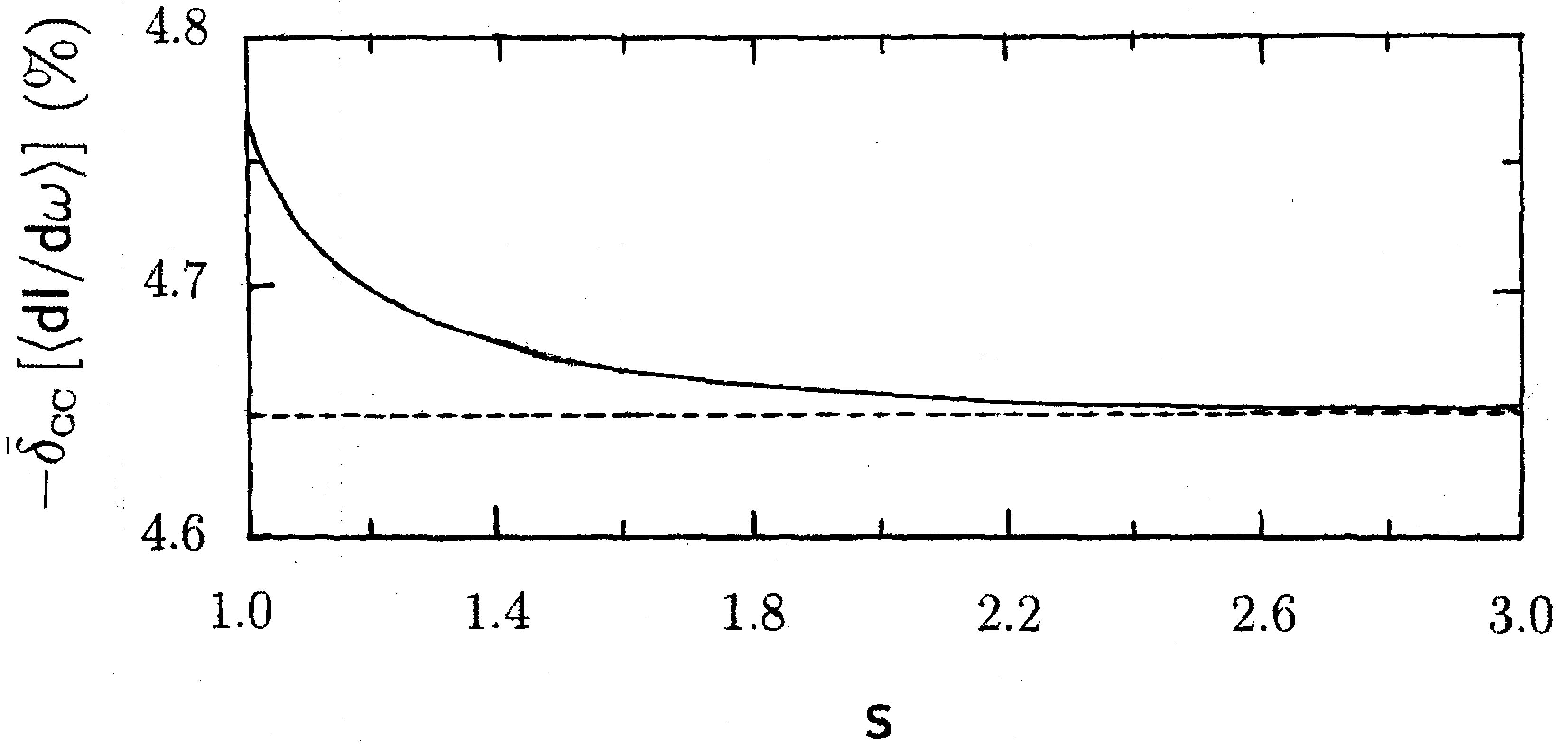
Figure 1: The $s$ dependence of the corrections $-\bar{\delta}_{\scriptscriptstyle CC}\left[\left\langle dI/d\omega\right\rangle\right]\,(\%)$ over the entire range $1.0\leq s\leq\infty$ of the parameter $s$.

Table 8 presents the values of the corrections $-{\delta}_{\scriptscriptstyle CC}\left[\left\langle dI/d\omega\right\rangle\right]\,(\%)$ for some separate high Z target elements over the range $1.0\leq s\leq\infty$.

Table 8. The dependence of $-\delta_{\scriptscriptstyle CC}\left[\langle dI/d\omega\rangle\right]$ values on the parameter $s$ in the regime of small LPM suppression for some high Z targets of experiment [25] at $\beta=1$ and $B^{\scriptscriptstyle B}=8.46$.

Target	$Z$	s=1.0	s=1.1	s=1.2	s=1.3	s=1.5	s=2.0	s=$\infty$
Au	79	0.0432	0.0428	0.0426	0.0424	0.0422	0.0421	0.0420
Pb	82	0.0458	0.0454	0.0451	0.0449	0.0447	0.0446	0.0445
U	92	0.0545	0.0540	0.0536	0.0534	0.0532	0.0530	0.0529

$\delta_{\scriptscriptstyle CC}\left[\left\langle\frac{dI}{d\omega}\right\rangle\right]$=$-4.50\pm 0.05\%$ ($Z$=$82$),   $\delta_{\scriptscriptstyle CC}\left[\left\langle\frac{dI}{d\omega}\right\rangle\right]$=$-5.35\pm 0.06\%$ ($Z$=$92$),

$\bar{\delta}_{\scriptscriptstyle CC}\left[\left\langle dI/d\omega\right\rangle\right]=-4.70\pm 0.49\%$.

Table 8 shows that averaging over the range $1.0\leq s\leq\infty$ corrections $\delta_{\scriptscriptstyle CC}\left[\langle dI/d\omega\rangle\right]$ for some separate high Z targets gives their sampling means $\delta_{\scriptscriptstyle CC}\left[\langle dI/d\omega\rangle\right]=-4.50\pm 0.05\%$ ($Z=82$) and $\delta_{\scriptscriptstyle CC}\left[\langle dI/d\omega\rangle\right]=-5.35\pm 0.06\%$ ($Z=92$), which coincide with the normalization correction values $-4.5\pm 0.2\%$ for $2\%L_{\scriptscriptstyle R}$ lead target and $-5.6\pm 0.3\%$ for $3\%L_{\scriptscriptstyle R}$ uranium target (Table II in [25]), respectively, within the experimental error.

Averaging over this range corrections $\bar{\delta}_{\scriptscriptstyle CC}\left[\left\langle dI/d\omega\right\rangle\right]$ gives the sampling mean $-4.70\pm 0.49\%$, which excellent agrees with the weighted average value $-4.7\pm 2\%$ of the normalization correction obtained in [25] for 25 GeV data. We believe that this allows one to understand the origin of the discussed in [24, 25] normalization problem for high Z targets.

3.4 Fokker–Planck approximation accuracy in the case $\boldsymbol{\omega}\mathbf{=0}$

Finally, let us briefly discuss the accuracy of the Fokker–Planck approximation that allows to obtain an analytical expression to be derived for the Migdal particle distribution function and the entire $\left\langle dI(\omega)/d\omega\right\rangle$ range to be rather simply calculate (using numerical calculation of triple integrals).

To this end, we will fix the parameter $a$ in expression (41) in such a way that the results of the exact calculation of $\left\langle dI(\omega)/d\omega\right\rangle\big{|}_{\omega\gg\omega_{cr}}$ and its calculation in the Fokker–Planck approximation coincide. As a result, we get

$$a=2\pi\biggl{(}\frac{Z\alpha\sigma}{m}\biggl{)}^{2}\biggl{(}\ln\frac{\sigma}{\theta_{a}}+\frac{7}{12}\biggl{)}\ .$$ (81)

Now we calculate $\left\langle dI(\omega)/d\omega\right\rangle\big{|}_{\omega=0}$ using the relations (41) and (81) and compare the result with the result obtained using ‘realistic’ (Molière) expression (26) for $\nu(\eta)$. Then for the ratio

$$R_{\scriptscriptstyle\mathrm{FPM}}=\frac{\left\langle dI(\omega)/d\omega\right\rangle_{\scriptscriptstyle\mathrm{FP}}}{\left\langle dI(\omega)/d\omega\right\rangle_{\scriptscriptstyle\mathrm{M}}}$$ (82)

we get the following values:

$$R_{\scriptscriptstyle\mathrm{FPM}}(\omega,L)=\left\{\begin{array}[]{cc}0.890,&L=0.007\,L_{\scriptscriptstyle\mathrm{R}}\\ 0.872,&L=0.060\,L_{\scriptscriptstyle\mathrm{R}}\end{array}\right.\ .$$ (83)

The values of corresponding relative corrections

$$\delta_{\scriptscriptstyle\mathrm{FPM}}\big{[}\!\left\langle dI/d\omega\right\rangle\!\big{]}=\frac{\left\langle dI(\omega)/d\omega\right\rangle_{\scriptscriptstyle\mathrm{FP}}-\left\langle dI(\omega)/d\omega\right\rangle_{\scriptscriptstyle\mathrm{M}}}{\left\langle dI(\omega)/d\omega\right\rangle_{\scriptscriptstyle\mathrm{M}}}$$ (84)

in percentage are given in Table 9.

Table 9. The relative correction $\delta_{\scriptscriptstyle\mathrm{FPM}}\big{[}\left\langle dI/d\omega\right\rangle\big{]}$ for $Z=79$ and $\omega=0$.

​L(cm)	$-\delta_{\scriptscriptstyle\mathrm{FPM}}\big{[}\left\langle dI/d\omega\right\rangle\big{]}\!$	$\!R_{\scriptscriptstyle\mathrm{FPM}}\big{[}\left\langle dI/d\omega\right\rangle\big{]}\!$
$\!0.007\,L_{\scriptscriptstyle\mathrm{R}}$	0.110​	​0.890​
$\!0.060\,L_{\scriptscriptstyle\mathrm{R}}$	0.128​	​0.872​

It is obvious that the relative difference between the Fokker–Planck approximation and the description based on the Molière theory $\delta_{\scriptscriptstyle\mathrm{FPM}}\big{[}\left\langle dI/d\omega\right\rangle\big{]}$ is about 12%, which is noticeably higher than the $3.2\%$ characteristic systematic experimental error [24].

Thus, the Fokker–Planck approximation and Gaussian distribution can not be used for describing the experimental data [24, 25] at low frequencies $\omega<30$ MeV. For their description the application of the Molière multiple scattering theory is advisable.

3.5 Coulomb corrections in the LPM effect theory analogue for a thin target

In [34] it is shown that the region of the emitted photon frequencies $\omega_{cr}>\omega>0$ naturally splits into two intervals, $\omega_{cr}>\omega>\omega_{c}$ and $\omega_{c}>\omega>0$, in first of which the LPM effect for sufficiently thick targets takes place, and in the second, there is its analogue for thin targets. The quantity $\omega_{c}$ is defined here as $\omega_{c}=2E^{2}/(m^{2}L)$.

Application of the Molière multiple scattering theory to the analysis of experimental data [24, 25] for a thin target in the second $\omega$ range is based on the use of the expression for the spatial-angle particle distribution function (11) which satisfies the standard Boltzmann transport equation for a thin homogeneous foil, and it differs significantly from the Gaussian particle distribution of the Migdal LPM effect theory.

Besides, it determines another expression for the spectral radiation rate in the context of the coherent radiation theory [34], which reads

$$\,\left\langle\frac{dI}{d\omega}\right\rangle=\int w_{\scriptscriptstyle\mathrm{M}}(\vartheta)\frac{dI(\vartheta)}{d\omega}d^{2}\vartheta\ .$$ (85)

Here

$$\frac{dI(\vartheta)}{d\omega}=\frac{2e^{2}}{\pi}\left[\frac{2\chi^{2}+1}{\chi\sqrt{\chi^{2}+1}}\ln\left(\chi+\sqrt{\chi^{2}+1}\right)-1\right]$$ (86)

with $\chi=\gamma\vartheta/2$. The latter expression is valid for consideration of the particle scattering in both amorphous and crystalline medium.

The formula (86) has simple asymptotes at the small and large values of parameter $\chi=\gamma\vartheta/2$:

$$\frac{dI(\vartheta)}{d\omega}=\frac{2e^{2}}{3\pi}\left\{\begin{array}[]{cl}\gamma^{2}\vartheta^{2},&\gamma\vartheta\ll 1\;,\\ 3\left[\ln(\gamma^{2}\vartheta^{2})-1\right],&\gamma\vartheta\gg 1\;,\end{array}\right.$$ (87)

Replacing $\vartheta^{2}$ by the average square value of the scattering angle $\overline{\vartheta^{2}}$ in this formula, we arrive at the following estimates for the average radiation spectral density:

$$\left\langle\frac{dI}{d\omega}\right\rangle=\frac{2e^{2}}{3\pi}\left\{\begin{array}[]{cl}\gamma^{2}\overline{\vartheta^{2}},&\gamma^{2}\overline{\vartheta^{2}}\ll 1\;,\\ 3\left[\ln(\gamma^{2}\overline{\vartheta^{2}})-1\right],&\gamma^{2}\overline{\vartheta^{2}}\gg 1\;.\end{array}\right.$$ (88)

In the experiment [24, 25], the above frequency intervals correspond roughly to the following $\omega$ ranges: $(\omega_{cr}>\omega>\omega_{c})\sim(244\,\mbox{MeV}>\omega>30\,\mbox{MeV})$ and $(\omega_{c}>\omega>0)\sim(30\,\mbox{MeV}>\omega>5\,\mbox{MeV})$ for 25 GeV electron beam and $0.7-6.0\%L_{\scriptscriptstyle\mathrm{R}}$ gold target. Whereas in the first area the discrepancy between the LPM theory predictions and data is about 3.2 to 5%, in the second area this discrepancy reaches $\sim 15\%$.

Using the approximate second-order representation of the Molière distribution function (24), (25) for computing the spectral radiation rate (85) the authors of [34] succeeded to agree satisfactorily theory and 25 GeV and $0.7\%L_{\scriptscriptstyle\mathrm{R}}$ data over the $\omega$ range 5 to 30 MeV.

This result can be understood by considering the fact that the correction to the Gaussian first-order representation of the distribution function $w_{\scriptscriptstyle\mathrm{M}}(\vartheta)$ of order of $1/B^{\scriptscriptstyle\mathrm{B}}$ is about 12% for the value used in calculations $B^{\scriptscriptstyle\mathrm{B}}=8.46$ [34].

Let us obtain the relative Coulomb correction to the averaged value of the spectral density of radiation for two limiting cases (88).

In the first case $\gamma^{2}\overline{\vartheta^{2}}\ll 1$, taking into account the equality

$$\delta_{\scriptscriptstyle\mathrm{CC}}[\gamma^{2}\overline{\vartheta^{2}}]=\delta_{\scriptscriptstyle\mathrm{CC}}[\overline{\vartheta^{2}}]\ ,$$ (89)

(71), and (88), we get

$$\delta_{\scriptscriptstyle\mathrm{CC}}\left[\left\langle\frac{dI}{d\omega}\right\rangle\right]=\delta_{\scriptscriptstyle\mathrm{CC}}\left[\left(\frac{dI}{d\omega}\right)_{0}\right]=\frac{f(\xi)}{1-B^{\scriptscriptstyle\mathrm{B}}}\ ,$$ (90)

where $B^{\scriptscriptstyle\mathrm{B}}\approx 8.46$ in the conditions of the discussed experiment [34].

In the second case $\gamma^{2}\overline{\vartheta^{2}}\gg 1$, we have

$$\Delta_{\scriptscriptstyle\mathrm{CC}}\left[\ln\left(\gamma^{2}\overline{\vartheta^{2}}\right)-1\right]=\Delta_{\scriptscriptstyle\mathrm{CC}}\left[\ln\left(\overline{\vartheta^{2}}\right)\right]=\Delta_{\scriptscriptstyle\mathrm{CC}}\big{[}\ln\left(B\right)\big{]}\ .$$ (91)

For the latter quantity, one can obtain

$$\Delta_{\scriptscriptstyle\mathrm{CC}}[\ln\left(B\right)]=\Delta_{\scriptscriptstyle\mathrm{CC}}[B]+f(Z\alpha)=\delta_{\scriptscriptstyle\mathrm{CC}}[B]\ .$$ (92)

The Coulomb correction then becomes

$$\Delta_{\scriptscriptstyle\mathrm{CC}}\left[\ln\left(\gamma^{2}\overline{\vartheta^{2}}\right)-1\right]=\frac{\delta_{\scriptscriptstyle\mathrm{CC}}[B]}{\left[\ln(\gamma^{2}\overline{\vartheta^{2}})^{\scriptscriptstyle\mathrm{B}}-1\right]}\ .$$ (93)

Taking into account (71), we arrive at a result:

$$\delta_{\scriptscriptstyle\mathrm{CC}}\left[\left\langle\frac{dI}{d\omega}\right\rangle\right]=\frac{f(\xi)}{\left[\ln(\gamma^{2}\overline{\vartheta^{2}})^{\scriptscriptstyle\mathrm{B}}-1\right]\Big{(}1-B^{\scriptscriptstyle\mathrm{B}}\Big{)}}\ .$$ (94)

The numerical values of these corrections are presented in Table 10.

Table 10. The relative Coulomb correction $\delta_{\scriptscriptstyle\mathrm{CC}}\big{[}\left\langle dI/d\omega\right\rangle\big{]}$ to the asymptotes of the Born spectral radiation rate over the range $\omega<\omega_{c}$ for $\beta=1$, $B^{\scriptscriptstyle\mathrm{B}}\approx 8.46$, and $\left(\gamma^{2}\overline{\vartheta^{2}}\right)^{\scriptscriptstyle\mathrm{B}}\approx 7.61$ [34].

Target	Z	$\gamma^{2}\overline{\vartheta^{2}}$	$-\delta_{\scriptscriptstyle\mathrm{CC}}\big{[}\left\langle dI/d\omega\right\rangle\big{]}$	$R_{\scriptscriptstyle\mathrm{CC}}$
Au	79	$\gamma^{2}\overline{\vartheta^{2}}\ll 1$	$0.042$	0.958
Au	79	$\gamma^{2}\overline{\vartheta^{2}}\gg 1$	$0.040$	0.960

The second asymptote is not reached [34] in the experiment [24, 25]. Therefore, we will now consider another limiting case corresponding to the experimental conditions and taking into account the second term of the Molière distribution function expansion (19).

Substituting the second-order expression (24) for the distribution function in (85) and integrating its second term (25), we can arrive at the following expression for the electron radiation spectrum at $\mu^{2}=\gamma^{2}\overline{\vartheta^{2}}\gg 1$ [34]:

$$\left\langle\frac{dI}{d\omega}\right\rangle=\frac{2e^{2}}{\pi}\left\{\ln\left(\mu^{2}\right)-C_{\scriptscriptstyle\mathrm{E}}\left(1+\frac{2}{\mu^{2}}\right)+\frac{2}{\mu^{2}}+\frac{C_{\scriptscriptstyle\mathrm{E}}}{B}-1\right\}\ .$$ (95)

In order to obtain the Coulomb correction to the Born spectral radiation rate from (95), we first calculate its numerical value at $(\mu^{2})^{\scriptscriptstyle\mathrm{B}}\approx 7.61$ and $B^{\scriptscriptstyle\mathrm{B}}\approx 8.46$, and we become $\left\langle dI/d\omega\right\rangle^{\scriptscriptstyle\mathrm{B}}=0.00542$. The Bethe–Heitler formula in the Born approximation gets $\left\langle dI/d\omega\right\rangle_{\scriptscriptstyle\mathrm{BH}}^{\scriptscriptstyle\mathrm{B}}=0.00954$.

Then, we calculate the numerical values of $B$ and $\mu^{2}$ parameters including the Coulomb corrections. From

$$\Delta_{\scriptscriptstyle\mathrm{CC}}[B]=\frac{f(\xi)}{1/B^{\scriptscriptstyle\mathrm{B}}-1}=-0.355\ ,$$ (96)

we obtain $B\approx 8.105$ for $Z=79$ and $B^{\scriptscriptstyle\mathrm{B}}\approx 8.46$. The equality

$$\Delta_{\scriptscriptstyle\mathrm{CC}}\left[\ln\mu^{2}\right]=\Delta_{\scriptscriptstyle\mathrm{CC}}\left[\ln B\right]=\Delta_{\scriptscriptstyle\mathrm{CC}}[B]+f(\xi)=\delta_{\scriptscriptstyle\mathrm{CC}}[B]=-0.042$$ (97)

gets $\ln\mu^{2}=1.987$ and $\mu^{2}=7.295$. Substituting these values in (95), we have $\left\langle dI/d\omega\right\rangle=0.00531$. The relative Coulomb corrections to these parameters are presented in Table 11. These corrections are not large. Their sizes are between two to four percent, i.e., of order of the experimental error.

Table 11. The relative Coulomb corrections in the analogue of the LPM effect theory for $0.07\,L_{\scriptscriptstyle\mathrm{R}}$ gold target, $\omega<\omega_{c}$, and $\beta=1$.

$\delta_{\scriptscriptstyle\mathrm{CC}}[B]$	$\delta_{\scriptscriptstyle\mathrm{CC}}\left[\ln\mu^{2}\right]$	$\delta_{\scriptscriptstyle\mathrm{CC}}\left[\left(dI/d\omega\right)_{\scriptscriptstyle 0}\right]$	$\delta_{\scriptscriptstyle\mathrm{CC}}\big{[}\left\langle dI/d\omega\right\rangle\big{]}$	$\delta_{\scriptscriptstyle\mathrm{CC}}\left[\Phi(s)\right]$
$-0.042$	$-0.021$	$-0.042$	$-0.020$	$-0.021$

Accounting for the relative Coulomb correction to the Bethe–Heitler spectrum of bremsstrahlung, we find $\left(dI/d\omega\right)_{\scriptscriptstyle\mathrm{BH}}=0.00916$. So we get

$$\left\langle\frac{dI}{d\omega}\right\rangle=0.580\left(\frac{dI}{d\omega}\right)_{\scriptscriptstyle\mathrm{BH}}\ .$$ (98)

This leads to the value of the spectral radiation rate in terms of $dN/[d(\log\omega)]$ $\times 1/L_{\scriptscriptstyle\mathrm{R}}$, where $N$ is the number of events per photon energy bin per incident electron, $dN/[d(\log\omega)/L_{\scriptscriptstyle\mathrm{R}}]=0.118\times 0.580=0.068$, which agrees very well with the experimental result over the frequency range $\omega<30$ MeV for 25 GeV and $0.7\%L_{\scriptscriptstyle\mathrm{R}}$ gold target. This result additionally improves the agreement between the theory and experiment (see Fig. 2). It is close to the Zakharov result [11] and coincides with the result of Blancenbeckler and Drell obtained in the eikonal approximation, which excellent agrees with $0.7\%L_{\scriptscriptstyle\mathrm{R}}$ 25 GeV data for $\omega>5$ MeV (see Figs. 12a in [25] and 20a in [26]).

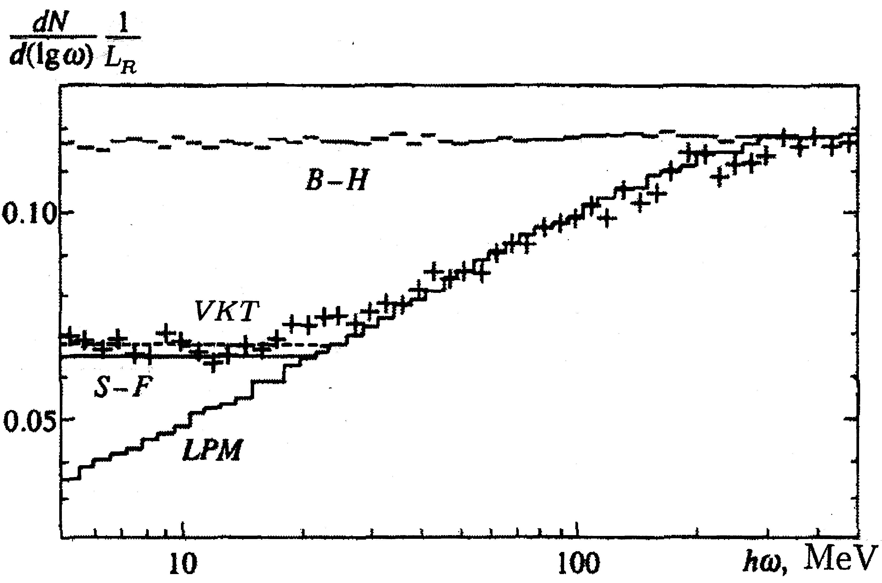
Figure 2: Measurement of the LPM effect over the range $30<\omega<500$ MeV and its analogue in the range $5<\omega<30$ MeV for the $0.7\%L_{\scriptscriptstyle R}$ gold target and 25 GeV electron beam. The signs ‘+’ denote the experimental data; the histograms B–H and LPM give the Bethe–Heitler and the LPM Monte Carlo predictions [24]. The solid and dashed lines (S–F and VKT) over the range $\omega<30$ MeV are the results of calculations without [34] and with the obtained Coulomb corrections.

Summary and conclusions

• Within the theory of LPM effect for finite-size targets, we calculated the Coulomb corrections to the Born bremsstrahlung rate and estimated the ratio $\left\langle dI(\omega)/d\omega\right\rangle/\left\langle dI(\omega)/d\omega\right\rangle^{\scriptscriptstyle\mathrm{B}}=R(\omega,L)$ for the gold target based on results of the revised Molière multiple scattering theory for the Coulomb corrections to the screening angle.

• We demonstrated that this $R(\omega,L)$ value is close to the normalization constant $R$ value for $0.7-6\%L_{\scriptscriptstyle\mathrm{R}}$ (25 GeV) data over the $\omega$ range 30 to 500 MeV from [10, 24]; however, the latter ignores the dependence of the ratio on $\omega$ and $L$.

• We obtained the analytical and numerical results for the Coulomb corrections to the function $\nu(\eta)=2\pi\int\sigma_{0}(\boldsymbol{\theta})[1-J_{0}(\eta\theta)]\boldsymbol{\theta}d\boldsymbol{\theta}$ and complex potential $U(\eta)=-\omega\lambda^{2}/2-i\,n_{0}\nu(\eta)$, and we showed that $-\delta_{\scriptscriptstyle\mathrm{CC}}\big{[}\nu(\eta)\big{]}=-\delta_{\scriptscriptstyle\mathrm{CC}}\big{[}U(\eta)\big{]}\sim 4.3\%<-\delta_{\scriptscriptstyle\mathrm{CC}}\big{[}\left\langle dI/d\omega\right\rangle\big{]}\sim 8.0\%$ for $Z=79$ ($\beta=1$).

• Additionally, we found Coulomb corrections to the quantities of the classical Migdal LPM theory, i.e., $\Delta_{\scriptscriptstyle\mathrm{CC}}\!\left[s\right]$, $\Delta_{\scriptscriptstyle\mathrm{CC}}\!\left[s^{2}\right]$, $\Delta_{\scriptscriptstyle\mathrm{CC}}\!\left[s^{4}\right]$, $\Delta_{\scriptscriptstyle\mathrm{CC}}\left[q\right]$, $\Delta_{\scriptscriptstyle\mathrm{CC}}\left[(dI/d\omega)_{0}\right]$, $\Delta_{\scriptscriptstyle\mathrm{CC}}\left[\Phi(s)\right]$, $\Delta_{\scriptscriptstyle\mathrm{CC}}\left[\langle dI/d\omega\rangle\right]$.

• We calculated relative Coulomb corrections $\delta_{\scriptscriptstyle\mathrm{CC}}\left[(dI/d\omega)_{0}\right]=\delta_{\scriptscriptstyle\mathrm{CC}}\left[q\right]$, $\delta_{\scriptscriptstyle\mathrm{CC}}\left[\Phi(s)\right]=\delta_{\scriptscriptstyle\mathrm{CC}}\left[s\right]$, and $\delta_{\scriptscriptstyle\mathrm{CC}}\left[\langle dI/d\omega\rangle\right]$ in the regime of strong LPM suppression for $Z=79$ ($\beta=1$). We showed that the latter correction $\delta_{\scriptscriptstyle\mathrm{CC}}\left[\langle dI/d\omega\rangle\right]$ comprises the order of $-14\%$ at minimum $B^{\scriptscriptstyle\mathrm{B}}$ value 4.5.

• We demonstrated that the average value $-5.4\%$ of the relative Coulomb correction for $Z=79$ coincides with the normalization correction value $-5.5\pm 0.2\%$ for $6\%L_{\scriptscriptstyle R}$ gold target obtained in experiment [25].

• We have performed the analogous calculations for the regime of small LPM suppression over the entire range $1\leq s\leq\infty$, and we found that the values of the Coulomb corrections $\delta_{\scriptscriptstyle CC}\left[\langle dI/d\omega\rangle\right]=-4.50\pm 0.05\%$ ($Z=82$) and $\delta_{\scriptscriptstyle CC}\left[\langle dI/d\omega\rangle\right]=-5.35\pm 0.06\%$ ($Z=92$) coincides with the values of the normalization correction $-4.5\pm 0.2\%$ for $2\%L_{\scriptscriptstyle R}$ lead target and $-5.6\pm 0.3\%$ for $3\%L_{\scriptscriptstyle R}$ uranium target, respectively, within the experimental error.

• The sample average over the range $1\leq s\leq\infty$, $\bar{\delta}_{\scriptscriptstyle CC}\left[\langle dI/d\omega\rangle\right]=-4.70\pm 0.49\%$, excellent agrees in the regime of small LPM suppression with the mean normalization correction $-4.7\pm 2\%$ obtained for 25 GeV data in the experiment [25].

• Thus, we managed to show that the discussed discrepancy between theory and experiment can be explained on the basis of the obtained Coulomb corrections to the Born bremsstrahlung rate within the Migdal LPM effect theory.

• This means that applying the revised multiple scattering theory by Molière allows one to avoid multiplying theoretical results by above normalization factor and leads to agreement between the Migdal LPM effect theory and experimental data [24, 25] for sufficiently thick high Z targets over the range $20<\omega<500$ MeV.

• We evaluated the accuracy of the Fokker–Planck approach and the Gaussian first-order representation of the distribution function $w_{0}(\boldsymbol{\vartheta})$ in the limiting case $\omega=0$, and we showed the need of the second-order correction of order of $1/B^{\scriptscriptstyle\mathrm{B}}\sim 12\%$ for $w(\boldsymbol{\vartheta})$ to eliminate the discrepancy between the theory and experimental data over the frequency range $5<\omega<30$ MeV for 25 GeV beam and $0.7\%L_{\scriptscriptstyle\mathrm{R}}$ gold target of the experiment [24, 25].

• Finally, we found the numerical results for the relative corrections $\delta_{\scriptscriptstyle\mathrm{CC}}\left[(dI/d\omega)_{0}\right]$, $\delta_{\scriptscriptstyle\mathrm{CC}}\left[\Phi(s)\right]$, and $\delta_{\scriptscriptstyle\mathrm{CC}}\left[\langle dI/d\omega\rangle\right]$ in the LPM effect theory analogue for a thin target over the range $5<\omega<30$ and demonstrated that these corrections additionally improve the agreement between the theory [33, 34] and experiment [24, 25].

Acknowledgments. This work is devoted to the memory of Alexander Tarasov. We would like to thank Spencer Klein (Lawrence Berkeley National Laboratory, USA) for valuable information and useful comments about some aspects of the SLAC E-146 experiment. We thank Bronislav Zakharov for drawing our attention to his more recent works [11]. We are grateful to Alexander Dorokhov for his attention to this work and reading the manuscript.

References

• [1]
• [2] Landau L.D., Pomeranchuk I.Ya. The limits of applicability of the theory of bremsstrahlung by electrons and of the creation of pairs at large energies // Dokl. Akad. Nauk. SSSR. 1953. V. 92. P. 535;
Landau L.D., Pomeranchuk I.Ya. Electron-cascade processes at ultra-high energies // Dokl. Akad. Nauk. SSSR. 1953. V. 92. P. 735.
• [3] Migdal A.B. The influence of the multiple scattering on the bremsstrahlung at high energies // Dokl. Akad. Nauk. SSSR. 1954. V. 96. P. 49.
• [4] Migdal A.B. Bremsstrahlung and pair production in condensed media at high energies // Phys. Rev. 1956. V. 103. P. 1811.
• [5] Goldman I.I. Bremsstrahlung at the boundary of a medium with account of multiple scattering // JETP. 1960. V. 38. P. 1866.
• [6] Baier V.N., Katkov V.M., Strakhovenko V.M. Radiation at collision of relativistic particles in media in the presence of external field // JETP. 1988. V. 67. P. 70;
Baier V.N., Katkov V.M. The theory of the Landau, Pomeranchuk, Migdal effect // Phys. Rev. D. 1998. V. 57. P. 3146.
• [7] Baier V.N., Katkov V.M., Fadin V.S. Radiation from Relativistic Electrons (in Russian). Atomizdat, Moscow: Atomizdat, 1973;
Baier V.N., Katkov V.M., Strakhovenko V.M. Electromagnetic Processes at High Energies in Oriented Single Crystals. Singapore: World Scientific Publishing Co, 1997.
• [8] Laskin N.V., Mazmanishvili A.S., Shul’ga N.F. Continual method in the problem of multiple scattering effect on radiation by high energy particle in amorphous media and crystals // Dokl. Akad. of Science of SSSR. 1984. V. 277. P. 850;
Laskin N.V., Mazmanishvili A.S., Shul’ga N.F. A method of path integration and Landau-Pomeranchuk effect of suppression of fast particle radiation in matter // Phys. Lett. A. 1985. V. 112. P. 240;
Akhiezer A.I., Laskin N.V., N.F. Shul’ga N.F. Method of functional integration in quantum theory of radiation by fast charged particles in matter // Dokl. Akad. of Science of SSSR. 1987. V. 295. P. 1363.
• [9] Zakharov B.G. Fully quantum treatment of the Landau–Pomeranchuk–Migdal effect in QED and QCD // JETP Lett. 1996. V. 63. P. 952;
Zakharov B.G. Light-cone path integral approach to the Landau–Pomeranchuk–Migdal effect // Phys. Atom. Nucl. 1998. V. 61. P. 838.
• [10] Zakharov B.G. Landau–Pomeranchuk–Migdal effect for finite-size targets // JETP Lett. 1996. V. 64. P. 781.
• [11] Zakharov B.G. Light-cone path integral approach to the Landau–Pomeranchuk–Migdal effect and the SLAC data on bremsstrahlung from high energy electrons // Yad. Fiz. 1999. V. 62. P. 1075.
• [12] Blancenbeckler R., Drell S.D. The Landau–Pomeranchuk–Migdal effect for finite targets // Phys. Rev. D. 1996. V. 53. P. 6265;
Blancenbeckler R. Structured targets and the Landau–Pomeranchuk–Migdal effect // Phys. Rev. D. 1997. V. 55. P. 190.
• [13] Blancenbeckler R. Multiple scattering and functional integrals // Phys. Rev. D. 1997. V. 55. P. 2441.
• [14] Shul’ga N.F., Fomin S.P. Suppression of radiation in an amorphous medium and in a crystal // JETP. Lett. 1978. V. 27. P. 117;
Shul’ga N.F., Fomin S.P. Theoretical and experimental investagations of the Landau–Pomeranchuk-Migdal effect in amorphous and crystalline matter // Probl. Atom. Sci. Technol. 2003. No. 2. P. 11;
Shul’ga N.F. Advances in Coherent Bremsstrahlung and LPM-Effect Studies // Int. J. Mod. Phys. A. 2010. V. 25. P. 9.
• [15] Gerhardt L., Klein S.R. Electron and Photon Interactions in the Regime of Strong LPM Suppression // Phys. Rev. D. 2010. V. 82. P. 074017.
• [16] Abbasi R. et al. (IceCube Collaboration). First Observation of PeV-energy Neutrinos with IceCube // Phys. Rev. Lett. 2013. V. 111. P. 021103;
Klein S.R. Radiodetection of Neutrinos // Nucl. Phys. B. Proc. Suppl. 2010. V. 00. P. 1–5.
• [17] Van Goethem M.J., Aphecetche L., Bacelar J.C.S. et al. Suppression of soft nuclear bremsstrahlung in proton-nucleus collisions // Phys. Rev. Lett. 2002. V. 88 P. 122302.
• [18] Sørensen, A.H. On the suppression of the gluon radiation for quark jets penetrating a dense quark gas // Z. Phys. C. 1992. V. 53. P. 595;
Brodsky S.J., Hoyer P. A bound on the energy loss of partons in nuclei // Phys. Lett. B. 1993. V. 298. P. 165;
Kopeliovich B.Z., Tarasov A.V., Schafer A. Bremsstrahlung of a quark propagating through a nucleus // Phys. Rev. C. 1999. V. 59. P. 1609.
• [19] Gyulassy M., Wang X.N. Multiple collisions and induced gluon bremsstrahlung in QCD // Nucl. Phys. B. 1994. V. 420. P. 583;
Gyulassy M., Levai P., Vitev I. Reaction operator approach to non-Abelian energy loss // Nucl. Phys. B. 2001. V. 594. P. 371.
• [20] Baier R., Dokshitzer Yu.L., Peignè S. et al. Induced gluon radiation in a QCD medium // Phys. Lett. B. 1995. V. 345. P. 277;
Baier R., Dokshitzer Yu.L., Mueller A.H. et al. The Landau–Pomeranchuk–Migdal effect in QED // Nucl. Phys. B. 1996. V. 478. P. 577;
Baier R., Dokshitzer Yu.L., Mueller A.H. et al. Medium-induced radiative energy loss; equivalence between the BDMPS and Zakharov formalisms // Nucl. Phys. B. 1998. V. 531. P. 403.
• [21] Baier V.N., Katkov V.M. Coherent and incoherent radiation from high-energy electron and the LPM effect in oriented single crystal // Phys. Lett. A. 2006. V. 353. P. 91.
• [22] Raffelt G., Seckel D. Multiple-scattering suppression of bremsstrahlung emission of neutrinos and axions in supernovae. // Phys. Rev. Lett. 1991. V. 67. P. 2605;
Pethick C.J., Thorsson V. Neutrino Pair Bremsstrahlung in Neutron Star Crusts: a Reappraisal // Phys. Rev. Lett. 1994. V. 72. P. 1964.
• [23] Baier R., Dokshitzer Yu.L., Mueller A.H. et al. Radiative energy loss of high energy quarks and gluons in a finite volume quark gluon plasma // Nucl. Phys. B. 1997. V. 483. P. 291;
Peignè S., Smilga A.V. Energy losses in relativistic plasmas: QCD versus QED // Phys. Usp. 2009. V. 179. P. 697.
• [24] Anthony P.L., Becker-Szendy R., Bosted P.E. et al. An accurate measurement of the Landau–Pomeranchuk–Migdal effect // Phys. Rev. Lett. 1995. V. 75. P. 1949;
Anthony P.L., Becker-Szendy R., Bosted P.E. et al. Measurement of dielectric suppression of bremsstrahlung // Phys. Rev. Lett. 1996. V. 76. P. 3550.
• [25] Anthony P.L., Becker-Szendy R., Bosted P.E. et al. Bremsstrahlung suppression due to the LPM and dielectric effects in a variety of targets // Phys. Rev. D. 1997. V. 56. P. 1373.
• [26] Klein S.R. Suppression of Bremsstrahlung and Pair Production due to Environmental Factors // Rev. Mod. Phys. 1999. V. 71. P. 1501.
• [27] Hansen H.D., Uggerhoj U.I., Biino C. et al. Landau–Pomeranchuk–Migdal effect for multihundred GeV electrons // Phys. Rev. D. 2004. V. 69. P. 032001.
• [28] Andersen J.U., Kirsebom K., Moller S.P. et al. (CERN-NA63 Collaboration). Electromagnetic Processes in Strong Cristalline Fields // Phys. Lett. B. 2009. V. 672. P. 323.
• [29] Tarasov A.V., Voskresenskaya O.O. An Improvement of the Molière–Fano Multiple Scattering Theory // Alexander Vasilievich Tarasov: To the 70th Birth Anniversary. Dubna: JINR, 2012. P. 276.
• [30] Kuraev E.A., Voskresenskaya O.O., Tarasov A.V. Coulomb Correction to the Screening Angle of the Molière Multiple Scattering Theory. JINR Preprint E2-2012-135. Dubna, 2012. 14 p.
• [31] Molière G. Theorie der Streuung schneller geladener Teilchen I. Einzelstreuung am abgeschirmten Coulomb-Feld // Z. Naturforsch. 1947. V. 2a. P. 133;
Molière G. Theorie der Streuung schneller geladener Teilchen II. Mehrfach- und Vielfachstreuung // Z. Naturforsch. 1948. V. 3a. P. 78.
• [32] Bethe H.A. Molière’s Theory of Multiple Scattering // Phys. Rev. 1953. V. 89. P. 256.
• [33] Shul’ga N.F., Fomin S.P. On the experimental verification of the Landau–Pomeranchuk–Migdal effect // JETP. Lett. 1996. V. 63. P. 873.
• [34] Shul’ga N.F., Fomin S.P. Effect of multiple scattering on the emission of ultrarelativistic electrons in a thin layer of matter // JETP. Lett. 1998. V. 113. P. 58.
• [35] Feynman R.P., Hibbs A.R. Quantum mechanics and path integrals. New York: McGrav-Hill, 1965.
• [36] Voskresenskaya O.O., Sisakian A.N., Tarasov A.V. et al. Theory of the Landau–Pomeranchuk Effect for Finite-Size Targets. JINR Preprint P2-97-308. Dubna, 1997. 8 p.; Tarasov A.V., Torosyan H.T., Voskresenskaya O.O. A quasiclassical approximation in the theory of the Landau–Pomeranchuk effect. ArXiv:1203.4853 [hep-ph].
• [37] Scott W.T. The Theory of Small-Angle Multiple Scattering of Fast Charged Particles // Rev. Mod. Phys. 1963. V. 35. P. 231.
• [38] Ter-Mikaelian M.L. Scatter of high energy electrons in crystals // Zh. Eksp. Teor. Fiz. 1953. V. 25. P. 289;
Ter-Mikaelian M.L. The interference emission of high-energy electrons // Zh. Eksp. Teor. Fiz. 1953. V. 25. P. 296;
Ter-Mikaelian M.L. High Energy Electromagnetic Processes in Condensed Media. New York: Wiley Interscience, 1972.
• [39]