Exploring Vortex Dynamics in the Presence of Dissipation: Analytical and Numerical Results

Abstract

In this paper, we examine the dynamical properties of vortices in atomic Bose-Einstein condensates in the presence of phenomenological dissipation, used as a basic model for the effect of finite temperatures. In the context of this so-called dissipative Gross-Pitaevskii model, we derive analytical results for the motion of single vortices and, importantly, for vortex dipoles which have become very relevant experimentally. Our analytical results are shown to compare favorably to the full numerical solution of the dissipative Gross-Pitaevskii equation in parameter regimes of experimental relevance. We also present results on the stability of vortices and vortex dipoles, revealing good agreement between numerical and analytical results for the internal excitation eigenfrequencies, which extends even beyond the regime of validity of this equation for cold atoms.

I Introduction

Much of the recent work regarding the emerging topic of nonlinear phenomena in Bose-Einstein condensates (BECs) has revolved around the theme of vortices. The latter constitute the prototypical two-dimensional (or quasi-two-dimensional) excitation that arises in BECs and bears a topological charge. The volume of work on BECs focusing on the theme of vortices can be well appreciated from the existence of many reviews on the subject fetter ; fetter2 ; newton_review ; our_review ; rcg:BEC_BOOK . Part of the fascination with vortices bears its roots in the significant connections of this field with other areas of Physics, including hydrodynamics nvortex_probl , superfluids Pismen1999 , and nonlinear optics yuri1 ; yuri2 .

While vortices chap01:vort2 ; chap01:vort3 ; foot and even robust lattices thereof chap01:latt1 ; chap01:latt2 ; chap01:latt3 were observed shortly after the experimental realization of BECs, recent years have shown a considerable increase in the interest in vortex dynamics. This is in good measure due to the activity of many experimental groups. Among them, we highlight the pioneering work of Ref. BPA_KZ enabling the formation of vortices through the so-called Kibble-Zurek mechanism kibble ; zurek2 ; the latter was originally proposed for the formation of large scale structure in the universe, by means of a quench through a phase transition. In Ref. BPA_KZ , the quench through the phase transition led to the BEC formation and hence to the spontaneous trapping of phase gradients and emergence of vortex excitations. In many of these experiments, not only single vortices, but also vortex dipoles were observed. This is where another remarkable contribution came to play freilich . By pumping a small fraction of the atoms to a different (unconfined by the magnetic trap) hyperfine state, it is possible to extract atoms (e.g. $\approx 5$% of the BEC) and image them, enabling for the first time (in BEC) a minimally destructive unveiling of the true vortex dynamics as it happens. This work and the follow-up efforts of Ref. pra_11 , as well as yet another remarkable experiment BPA_10 revealed the key dynamical relevance of multi-vortex clusters in the form of vortex dipoles (VDs). In the experiment of Ref. BPA_10 , the superfluid analogue of flow past a cylinder was realized, leading to the spontaneous emergence of such VDs. In Ref. pra_11 , the full (integrable at the level of two vortices) dynamics of the VD case was revealed. The theme of few-vortex crystals has garnered interest in the case of higher number-of-vortices variants in the works of Ref. bagnato (3 vortices) and in the very recent co-rotating (same charge) vortex case of Ref. corot (3 as well as 4 same charge vortices).

On the other hand, another topic of increasing attention has concerned the role of finite-temperature induced damping of the BEC Proukakis_Book that, in turn, leads to anti-damping in the motion of the coherent structures therein. In particular, the simpler case of dark solitons in single-component BECs has been studied at some length shl1 ; shl2 ; us ; ft1 ; ft2 ; ft3 ; ft4 ; gk ; ashton . In this context, the work of Ref. shl1 (see also Ref. shl2 ) provided originally a kinetic-equation along with a study of the Bogolyubov-de Gennes (BdG) equations. There, it was argued that the dark soliton obeys an anti-damped harmonic oscillator equation, resulting into trajectories of growing oscillating amplitudes around the center of the trap confining the BEC: the first experiments han1 ; han2 ; nist observed the motion of a dark soliton created by phase imprinting at the center of the trap towards the edge of the trap nist ; one/more full soliton oscillations were subsequently demonstrated in two distinct experiments bongs ; heidelberg (see also related theoretical work of Refs. ba00 ; freq ). More recently, the effect of anti-damping was actually directly observed for the first time  Zwierlein in the related context of dark soliton oscillations in the unitary Fermi gas.

Anti-damped dynamical equations for dark solitons (in the context of bosons) were derived in Ref. us by means of a Hamiltonian perturbation approach djf applied to the dissipative variant of the Gross-Pitaevskii equation (DGPE). The DGPE was originally introduced phenomenologically by Pitaevskii lp as a simplified means of accounting (through a damping term) for the role of finite temperature induced fluctuations in the condensate dynamics; see, e.g., Refs. penckw ; Proukakis_Book ; npprev ; blakie ; ZNG_Book for the microscopic interpretation of such a term. It should be noted here that, at least in the dark soliton context, the DGPE model was found us to yield predictions that compared favorably with more complex stochastic Gross-Pitaevskii equation (SGPE) stoof_sgpe ; stoch when comparing to appropriately averaged quantities with the same dissipation parameter; for this reason, we adopt the DGPE in what follows. The DGPE has been employed in more complex settings involving multiple dark solitons dcdss and dark-bright solitons in multiple component BECs njp , yet it has arguably received somewhat less attention in higher dimensions, and especially so in the case of single- and multiple vortex states. The dynamics of vortices under the influence of thermal effects, has been considered in some computational detail recently proukv1 ; proukv2 ; ourjpb ; ashtone ; tmwright , and a semi-classical limit case in the absence of a trap has been of mathematical interest as well spirn ; miot (see also Ref. stamp for the role of quantum effects, mostly relevant at extremely low temperatures, as well as atom numbers, where they dominate over thermal effects). While the case of a single trapped vortex has been considered in the pioneering work of Ref. stoof (see also Ref. ashtone2 ), a comparison of numerical computations to analytical results, and more importantly, its generalization to multi-vortex settings is still an open problem; it is the aim of the present work to contribute towards this direction.

We start by developing in Sec. II an energy-based method that provides a dynamical equation characterizing the single vortex dynamics, with our results also supplemented by another technique (cf. Appendix A) based on methods similar to the ones of Refs. spirn ; miot . We believe that our method provides a useful alternative to the approach of Ref. stoof (the relevant connections are discussed herein). The main focus of this paper (Sec. III) is to generalize this to the experimentally relevant case of a vortex dipole, using the relevant set of first-order ordinary differential equations (ODEs). The resulting ODEs are then compared to the full DGPE model. We also perform a linear stability analysis in the absence/presence of the phenomenological damping, and characterize the internal modes of the single and dipole vortex systems (cf. Appendix B). Our results for the single vortex and vortex dipole stability and dynamics reveal the following: already in the regime of small but experimentally-relevant chemical potentials, where the vortices can be well approximated as particles fully characterized by their position, the model provides a qualitatively accurate and semi-quantitative approximation of the relevant stability and dynamical properties of the original equation (DGPE) for typical low temperature BEC experiments. We summarize and discuss the broader context of our results in Sec. IV.

II Single Vortex Solutions of the Dissipative Gross-Pitaevskii Equation

The dissipative GPE model can be expressed in the following dimensionless form for a pancake shaped BEC (see e.g., Ref. ourjpb for the reductions that lead to such a quasi-two-dimensional description)

$$(i-\gamma)u_{t} = -\frac{1}{2}\Delta u+V(r)u+|u|^{2}u-\mu u.$$ (1)

Here, $u$ represents the quasi-two-dimensional BEC wavefunction, $\Delta$ represents the Laplacian operator, $V(r)=\frac{1}{2}\Omega^{2}r^{2}$ is the external harmonic trap ($\Omega$ is the normalized trap frequency, while $r^{2}=x^{2}+y^{2}$), and $\mu$ stands for the chemical potential. The latter is directly related to the number of atoms in the BEC, with the limit of large $\mu$ being suitable for a particle-based description of coherent structures (in a semi-classical fashion; see e.g., Ref. coles ). Finally, the dimensionless parameter $\gamma$ is associated with the system’s temperature, based on the earlier treatment of Ref. penckw —see also Refs. Proukakis_Book ; npprev ; blakie ; ZNG_Book ; stoof for more details. Physically relevant cases correspond to $\gamma\ll 1$ footnote1 , as also discussed in the specific applications of Refs. us ; ft1 ; ft3 .

In the case of a single vortex, the stationary state is well-known to exist at the center of the parabolic trap; in the Hamiltonian case of $\gamma=0$, upon displacement from the trap center, the vortex executes a circular precession around it fetter which has been also very accurately quantified experimentally freilich . However, for $\gamma\neq 0$, the anomalous (internal) mode of the vortex associated with the precessional motion becomes unstable. This anomalous mode, as explained, e.g., in Ref. ourjpb , is associated with the fact that the vortex does not represent the ground state of the system. Nevertheless, it is a dynamically stable entity in the absence of a dissipative channel, as it cannot shed energy away to spontaneously turn into the ground state. Yet, as was rigorously proved in Ref. sandst , the existence of any dissipation typically renders such anomalous modes (so-called negative Krein sign modes) immediately unstable, as it provides a channel enabling the expulsion of the coherent structure and the conversion of the system into its corresponding ground state. This is evident from the presence of a positive imaginary part of the eigenfrequency (i.e., a real part of the corresponding eigenvalue), which directly signals the relevant instability for any non-zero value of $\gamma$. This is discussed further in Appendix B, which also shows how the spectrum of the Hamiltonian ($\gamma=0$) case gets modified by $\gamma$.

Motivated by the above discussion (and corresponding numerical results in Appendix B), we now develop a systematic approach based on the time evolution of the vortex energy for accounting the effect of the anti-damping term proportional to $\gamma$. In particular, we will seek to identify the equations of motion for the center of a single vortex $(x_{0},y_{0})$ as a first step towards investigating the vortex dipole case.

In the case of $\gamma=0$, the energy of the system [i.e., the Hamiltonian associated with Eq. (1)] reads:

$$E=\frac{1}{2}\iint\left\{\left(|u_{x}|^{2}+|u_{y}|^{2}\right)+(|u|^{2}\!-\!\mu)^{2}+2V|u|^{2}\right\}dx\,dy.$$ (2)

It is then straightforward to confirm by means of direct calculation that, in the case of $\gamma\neq 0$,

$$\frac{dE}{dt}=-2\gamma\iint|u_{t}|^{2}dx\,dy,$$ (3)

which forms the starting point of our analysis.

II.1 Single Vortex Dynamics

For the case of a single vortex inside the BEC, it can be found lundh that the energy reads:

$$E= \frac{\pi\rho_{0}}{2}\left[\left(1-\frac{r_{0}^{2}}{R_{\rm TF}^{2}}\right)\log\left(\frac{R_{\rm TF}^{2}}{\xi_{0}^{2}}\right)\right.$$

$$+\left.\left(\frac{R_{\rm TF}^{2}}{r_{0}^{2}}+1-2\frac{r_{0}^{2}}{R_{\rm TF}^{2}}\right)\log\left(1-\frac{r_{0}^{2}}{R_{\rm TF}^{2}}\right)\right],$$ (4)

where $r_{0}=\sqrt{x_{0}^{2}+y_{0}^{2}}$ and $(x_{0},y_{0})$ is the location of the vortex center, $R_{\rm TF}=\sqrt{2\mu}/\Omega$ is the Thomas-Fermi radius, $\rho_{0}=\mu$ and $\xi_{0}=(2\mu)^{-\frac{1}{2}}$ are, respectively, the density and the value of the healing length at the trap center. For small $r_{0}/R_{\rm TF}$, i.e., for vortices close to the trap center, the first term in Eq. (4) dominates and thus:

$$E\approx\frac{\pi\rho_{0}}{2}\left(1-\frac{r_{0}^{2}}{R_{\rm TF}^{2}}\right)\log\left(\frac{R_{\rm TF}^{2}}{\xi_{0}^{2}}\right).$$ (5)

Then, we have

$$\frac{dE}{dt} \approx \frac{\pi\rho_{0}}{2}\left[\log\left(\frac{R_{\rm TF}^{2}}{\xi_{0}^{2}}\right)\left(-\frac{1}{R_{\rm TF}^{2}}\right)(2x_{0}\dot{x}_{0}+2y_{0}\dot{y}_{0})\right]$$ (6)

$$\approx -\omega_{\rm pr}(2x_{0}\dot{x}_{0}+2y_{0}\dot{y}_{0})$$

where $\omega_{\rm pr}=\frac{\pi\rho_{0}}{2}\log(\frac{R_{\rm TF}^{2}}{\xi_{0}^{2}})(\frac{1}{R_{\rm TF}^{2}})$ is an approximation to the vortex precession frequency.

Now, we turn our attention to the right hand side of Eq. (3). Starting from Eq. (1) with $\gamma=0$ and substituting the following polar representation of a single vortex $u(r,\theta)=\sqrt{\rho(r)}\,e^{i\theta}$ to Eq. (1), we obtain the familiar ODE for the radial vortex profile:

$$\rho^{\prime\prime}-\frac{\rho^{\prime 2}}{2\rho}+\frac{\rho^{\prime}}{r}-\frac{2\rho}{r^{2}}+4\left[\mu-\rho-V(r)\right]\rho = 0.$$ (7)

The proposed form for $\rho$ (from a Padé approximation —see e.g., Ref. berloff ) is:

$$\rho(r) = \frac{r^{2}(a_{1}+a_{2}r^{2})}{1+b_{1}r^{2}+b_{2}r^{4}}e^{-\Omega^{2}r^{2}},$$ (8)

where $a_{2}=\mu b_{2}$. The coefficients $a_{1}$, $b_{1}$, and $b_{2}$ computed by substitution for different choices of chemical potential $\mu$ considered before, and for a trap frequency of $\Omega=0.2$, are depicted in Table 1.

$\mu$	$a_{1}$	$a_{2}$	$b_{1}$	$b_{2}$
0.4	0.06698	0.01470	0.3795	0.03676
0.8	0.3676	0.05004	0.4961	0.0625
1	0.6021	0.0972	0.6215	0.0972
1.6	1.6359	0.4123	1.0121	0.2577

Table 1: Coefficients for the Padé approximation (8) of a unitary charge vortex for different values of the chemical potential $\mu$ for a trap strength of $\Omega=0.2$.

A subsequent substitution and direct evaluation for the right hand side of Eq. (3) reads as follows:

$$-2\gamma\iint|u_{t}|^{2}dx\,dy$$

$$\qquad=-2\gamma\iint|u_{t}(x-x_{0}(t),y-y_{0}(t))|^{2}dx\,dy$$

$$\qquad=-2\gamma\iint\left(\frac{\partial v}{\partial\xi}(-\dot{x}_{0})+\frac{\partial v}{\partial\eta}(-\dot{y}_{0})\right)$$

$$\quad\qquad\qquad\qquad\left(\frac{\partial v^{*}}{\partial\xi}(-\dot{x}_{0})+\frac{\partial v^{*}}{\partial\eta}(-\dot{y}_{0})\right)d\xi\,d\eta$$

$$\qquad=-2\gamma\left(\dot{x}_{0}^{2}s+\dot{y}_{0}^{2}s\right)$$ (9)

where

$$s=\iint\frac{\partial v}{\partial\xi}\frac{\partial v^{*}}{\partial\xi}=\iint\frac{\partial v}{\partial\eta}\frac{\partial v^{*}}{\partial\eta},$$ (10)

and ${\rm Re}(\iint\frac{\partial v}{\partial\eta}\frac{\partial v^{*}}{\partial\xi})=0$. Here, we have used the variables $\xi=x-x_{0}(t)$ and $\eta=y-y_{0}(t)$, so that $v(\xi,\eta)=u(x-x_{0}(t),y-y_{0}(t))$. The resulting integral constant $s$ can be directly evaluated using the above Padé approximation $u=\sqrt{\rho}\,e^{i\theta}$, finding that $s=0.5864,1.5977,2.1003,3.5911$ for $\mu=0.4,0.8,1,1.6$ respectively.

Using the above results at hand, one can combine the left and right hand side of Eq. (3) and obtain

$$\omega_{\rm pr}(x_{0}\dot{x}_{0}+y_{0}\dot{y}_{0})=s\gamma\left(\dot{x}_{0}^{2}+\dot{y}_{0}^{2}\right).$$ (11)

From this, we can infer the equations of motion of the single vortex state. Looking for equations of motion that correspond to rotation with anti-damping, we add a term proportional to $\dot{x}_{0}\dot{y}_{0}$ to both sides of Eq. (11) and split it into the following two equations:

$$\omega_{\rm pr}x_{0}+\dot{y}_{0} = s\gamma\dot{x}_{0},$$ (12)

$$\omega_{\rm pr}y_{0}-\dot{x}_{0} = s\gamma\dot{y}_{0}.$$ (13)

Then, the analytical expression for the complex eigenfrequency $\omega=\omega_{r}+i\,\omega_{i}$ is

$$\omega_{i} ={\rm Im}(\omega) =\frac{\omega_{\rm pr}s\gamma}{1+(s\gamma)^{2}},$$ (14)

$$\omega_{r} ={\rm Re}(\omega) =\frac{\omega_{\rm pr}}{1+(s\gamma)^{2}}.$$ (15)

At this level of approximation, the vortex (outward spiraling) trajectories can be given explicitly as:

$$x = e^{\omega_{i}t}\left[y_{0}\sin\left(\omega_{r}t\right)+x_{0}\cos\left(\omega_{r}t\right)\right],$$ (16)

$$y = e^{\omega_{i}t}\left[y_{0}\cos\left(\omega_{r}t\right)-x_{0}\sin\left(\omega_{r}t\right)\right].$$ (17)

This is a result which parallels the one derived for the case of the dark soliton (see, e.g., Ref. us ). We now provide a number of connections of this to earlier analytical considerations.

First, we should note that our approach here is based on a particle picture that is most suitable to use in the semi-classical or Thomas-Fermi limit of large $\mu$. As discussed, e.g., in Ref. coles , this is the regime where it is relevant to consider the vortex as a “particle” without internal structure, characterized solely by $(x_{0},y_{0})$. On the other hand, earlier works stoof ; ashtone2 have explored both dissipative and stochastic effects on the motion of the vortex, but in a different regime wherein the wavefunction can be approximated in a Gaussian form note . The latter is applicable closer to the linear regime of the system. In light of these differences, we will not attempt a direct comparison of these predictions, but we do note the close proximity of the final result of Eqs. (12)-(13) with, e.g., Eq. (25) in Ref. stoof . Moreover, using the dimensional estimates presented therein, we evaluate typical values of the parameter $\gamma$ in the regime $0.00023$–$0.0023$ for temperatures of the order of $10$–$100$ nK. Our present work will focus on the two cases of $\gamma=0$ (no damping), and $\gamma=0.0023$, which represents an upper “realistic” limit for experiments, beyond which the use of the DGPE may not be well justified for the particular physical system.

An additional class of techniques for deriving such effective equations, also based on conservation laws, has been developed from a rigorous perspective in Refs. spirn ; miot . However, the latter work considers settings where the vortices evolve on a homogeneous background in the absence of a trap. More recently, these rigorous methods have been explored in the presence of a trap as well jerrard . In Appendix A we provide an outline of how to utilize this class of methods in the current setting. This, in turn, leads to a result similar to the one obtained above in Eqs. (12)-(13) and thus further corroborates our theoretical predictions.

II.2 Vortex Dipole Dynamics

The above considerations can be generalized to the case of the vortex dipole following a similar approximation as the one used in Ref. pra_11 . In particular, if we assume that the effect of interaction of the “point vortices” (in the large chemical potential regime) is independent of the anti-damped motion of each single vortex, then the equations of motion combining the two effects for the vortices constituting the dipole state read:

$$\dot{x}_{1} = -S_{1}\omega_{\rm pr,1}y_{1}-BS_{2}\frac{y_{1}-y_{2}}{2\rho_{12}^{2}}+s\gamma\dot{y}_{1},$$ (18)

$$\dot{y}_{1} = \phantom{-}S_{1}\omega_{\rm pr,1}x_{1}+BS_{2}\frac{x_{1}-x_{2}}{2\rho_{12}^{2}}-s\gamma\dot{x}_{1},$$ (19)

$$\dot{x}_{2} = -S_{2}\omega_{\rm pr,2}y_{2}-BS_{1}\frac{y_{2}-y_{1}}{2\rho_{12}^{2}}-s\gamma\dot{y}_{2},$$ (20)

$$\dot{y}_{2} = \phantom{-}S_{2}\omega_{\rm pr,2}x_{2}+BS_{1}\frac{x_{2}-x_{1}}{2\rho_{12}^{2}}+s\gamma\dot{x}_{2},$$ (21)

where the centers of the vortices are $(x_{1},y_{1})$ and $(x_{2},y_{2})$, with respective charges $S_{1}=1$ and $S_{2}=-1$, and $s$ defined similarly as in the case of the single vortex case. For the rest of our analysis, in order to capture the precession frequency increase as we depart from the BEC center and approach its outer rim, we will consider a slightly modified form for the precession frequency for each vortex used by Ref. pra_11 :

$$\omega_{\rm pr,i}=\frac{\omega_{\rm pr}}{1-\frac{r_{i}^{2}}{R_{\rm TF}^{2}}},$$ (22)

where $r_{i}=\sqrt{x_{i}^{2}+y_{i}^{2}}$ is the distance of each vortex to the trap center, $\omega_{\rm pr}=\frac{\Omega^{2}}{2\mu}\log{\frac{A\mu}{\Omega}}$ is the precession frequency close to the trap center, and $A=8.88$. Finally, the coefficient $B$ is a factor that takes into account the screening of the vortex interaction due to the modulation of the density within the Thomas-Fermi background cloud in which the vortices are seeded. In the case of a homogeneous background, $B=2$ which will be adopted for cases of sufficiently large chemical potential (such as $\mu=4$) herein. For modulated densities this value needs to be suitably modified; see, e.g., Ref. busch for the form of the interaction in the latter case. Here, adopting an approach similar to that of Ref. middel2 , we use an effective $B=1.35$ for computations with considerably lower chemical potentials (such as $\mu\leq 1.6$). This approach has been shown to yield accurate results for multi-vortices in the case of $\gamma=0$ pra_11 .

The effective equations of motion for two opposite charge vortices (18)–(21) admit a steady state solution corresponding to a stationary VD pra_11 . The equilibrium positions for the VD are $(x_{\rm eq},y_{\rm eq})=(0,\pm\frac{B}{4\omega_{\rm pr}+{B}/{R_{\rm TF}^{2}}})$. In the next section we investigate the dynamics of single vortices and VDs in the presence of the phenomenological dissipation and we compare them with predictions from the analytical results obtained in this section.

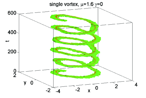
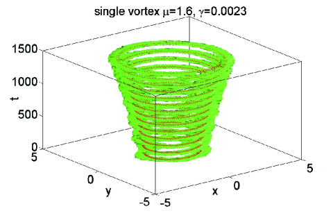
Figure 1: (Color online) Isosurfaces of anti-damped single vortex motion for $\gamma=0$ (left) and $\gamma=0.0023$ (right), showing the full PDE [Eq. (1)] numerical results (green) and the analytical result obtained from the vortex ODEs (red). Here, the initial position is $(x_{0},y_{0})=(0,1.5)$, the chemical potential $\mu=1.6$ and the trap frequency $\Omega=0.2$.

We now turn to numerical computations to examine the validity of our analytical approximations.

III Numerical Results

We start by briefly discussing the key findings concerning the predictions of the eigenfrequencies of the unstable system and their dependence on the phenomenological dissipation parameter, with further details left to Appendix B.

Both in the cases of a single vortex and a symmetric vortex dipole, we observe good agreement of our theoretical prediction with the anomalous mode (complex) frequency associated with the vortex motion over the regime of physical relevance of the DGPE; mathematically, this agreement actually extends far beyond the physically relevant $\gamma\ll 1$ regime, a feature presumably associated with the non-perturbative nature of our approach. On the other hand, we find the method to be most accurate in the case of large chemical potential, where the vortex can be characterized as a highly localized “particle” (a nearly point vortex without internal structure), while it is less successful very close to the linear limit of the problem. Moreover, the relevant complex pair of eigenfrequencies corresponding to the anomalous mode never becomes real, i.e., the motion always remains a spiral one independently of the strength of the dissipation parameter. We highlight this here, as it is in contrast to what is known in one-dimension for the case of the dark soliton: in the latter case, for sufficiently large $\gamma$, an over-damped regime of exponential expulsion of the dark soliton emerges us .

We now turn to the dynamical evolution of both the single vortex and the counter-rotating vortex pair. To that effect, we resort to direct numerical integration of Eq. (1) for these states. In order to determine the position of the vortex as a function of time, we compute the fluid velocity

$$v_{s} = -\frac{i}{2}\frac{u^{*}\nabla{u}-u\nabla{u^{*}}}{|u|^{2}}$$ (23)

and the fluid vorticity is defined as $\omega_{\rm vor}=\nabla\times v_{s}$. Since the direction of the fluid vorticity is always the $z$-direction, we can treat it as a scalar. We can determine the position of the vortex via a local center of mass of the vorticity $\omega_{\rm vor}$ (around its maxima or minima). However, in what follows, we represent the vorticity iso-contours, which also enables us to explore the full (2+1)-dimensional space-time motion $(x,y,t)$ of the vortex.

Figure 1 compares the full space-time vorticity dynamics of the single vortex for $\gamma=0$ (i.e., the Hamiltonian case of pure condensate) with the “finite temperature” case of $\gamma=0.0023$. The figure compares the actual vorticity isocontours (thick green lines) to the theoretical prediction based on our ODEs of Eqs. (12)-(13) for the respective $\gamma$ (red lines). On the whole, agreement for the single vortex case is extremely good in all cases studied. As evident from the figure for any $\gamma>0$, the “particle” ODEs yield a well-defined anti-damped pattern, whereas the full numerical simulation reveals a small amount of modulation on top of the underlying trajectory —this is presumably related to the (nonlinear) role of continuous vortex-sound interactions within a trap (anticipated to be at most of order few $\%$ ft1 ) which is not accounted for in our analytical model. In addition to this, closer inspection reveals a very slight deviation (typically less than $1\%$ in the case of a single vortex) in the evolution timescales, associated with tiny shifts in both the amplitude and the frequency of the anti-damped motion. As anticipated, the agreement improves further with increasing values of $\mu$, and as such deviations are not expected to lead to any experimentally noticeable effects, they will not be discussed any further here.

The situation becomes slightly more complicated in the case of a vortex dipole (Fig. 2), as both the vortex anti-damped motion and the vortex-sound interactions acquire an additional channel associated with the vortex-vortex (and, indirectly, sound-sound) interactions prouk12 . Here we need to distinguish two cases, based on the symmetry of the case under study (or its absence).

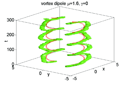
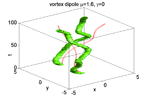
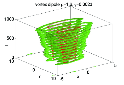
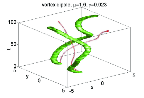
Figure 2: (Color online) Motion for a symmetric (left column) and an asymmetric (right column) vortex dipole in the absence (top panels) and presence (bottom panels) of dissipation. The initial positions of the two vortices are: Left Column: $(x_{1},y_{1})=(0,1.75),(x_{2},y_{2})=(0,-1.75)$, Right Column: $(x_{1},y_{1})=(0,3.00),(x_{2},y_{2})=(0,-1.25)$, while the chemical potential $\mu=1.6$ and the trap frequency $\Omega=0.2$. Other parameters as in Fig. 1.

Figure 3: (Color online) Left four panels: Analytical versus numerical trajectories of the vortex dipole epicycle for $\mu=4$, $\gamma=0$, $\Omega=0.1$, $B=2$ case. In particular, the upper left subpanel is the three-dimensional comparison of the vortex instantaneous positions $(x,y)$ versus $t$, the upper right subpanel is the projection of the motion on the $(x,y)$ plane, the bottom left subpanel is the projection on the $(y,t)$ plane and the bottom right subpanel is the projection on the $(x,t)$ plane. Here the thick blue and green lines correspond to the analytical predictions while the thin red and black lines correspond to the numerical results. Right four panels: As in the left panels, but with $\gamma=0.0023$.

Initially, we consider the case of a symmetric vortex dipole (Fig. 2, left column), focusing for consistency on the same parameters as for the single-vortex case (Fig. 1), where excellent agreement has already been reported; here, we effectively excite the epicyclic precession mode of the vortex dipole. We find that for the relatively small chemical potentials $\mu\sim O(1)$ considered here, there is a small noticeable deviation even for $\gamma=0$; this is presumably due to the neglect of vortex-sound interactions in the analytical model. We note that in the case of finite $\gamma$, the epicyclic trajectory will continue to expand outward until the vortices essentially merge with the vanishing background of the cloud and disappear thereafter; here, the corresponding analytical anti-damped pattern ($\gamma\neq 0$) consistently predicts a slightly lower amplitude of oscillations, with the discrepancy increasing with increasing $\gamma$ (at constant small value of $\mu$). However, a slight increase in the value of $\mu$ can considerably suppress such differences (see subsequent Fig. 3 and related discussion).

Fig. 2 also shows the case of an asymmetric vortex dipole (right columns), revealing that this deviation becomes more pronounced in this case, with an increase in the relative difference in off-centered locations of the two vortices amplifying such an effect. To display this effect, we have chosen to show here a highly asymmetric initial VD configuration, which nonetheless yields reasonable qualitative agreement.

In particular, Fig. 2 (top right panel) shows that in the Hamiltonian case of $\gamma=0$, one of the vortices rotates closer to the trap center, while the other one precesses further outside. On the other hand, in the presence of anti-damping (bottom right panel), the vortices rapidly spiral towards the Thomas-Fermi radius and cannot be accurately tracked thereafter. It is important to note that in this case, involving dynamics of the vortices fairly close to the Thomas-Fermi radius, we have generally found (in dynamical evolutions not shown herein) that our theoretical analysis and particle model are least likely to properly capture the vortex dynamics. This is because in this case the condensate’s density modulation in fact affects most significantly both of the dynamical elements contained in our model, namely the precession and the inter-vortex interaction. As regards the precession, we have found that Eq. (22) is progressively less accurate for distances approximately satisfying $r>0.7R_{\rm TF}$. At the same time, this density modulation most significantly affects the screening effect discussed above (and detailed, e.g., in Ref. busch ). As a result, in settings such as those of Fig. 2 (right column) we may expect a rough qualitative agreement between the numerical observations and our simple ODE model, but a quantitative match would require a considerably more complex particle model accounting for the above traits, which is beyond the scope of the present work.

We note that this trend seen in the dependence of the VD motion is in qualitative agreement with previous findings in the related case of two interacting dark solitons in a single harmonic trap. In particular, Ref. allen_soliton , highlighted the increased role of soliton-sound interactions for two solitons located in asymmetric positions in a one-dimensional harmonic trap, which allowed significant energy exchange.

In the spirit of exploring the relevance of the model to other parametric regimes, we have also attempted to probe similar features, as e.g. in Fig. 2, for different sets of parameter values. Our conclusion from this study is that for larger values of the chemical potential and smaller values of the trap frequency $\Omega$, the model becomes generally and progressively more accurate. This is confirmed not only by the eigenvalue computations and more accurate linearization predictions (see Appendix B), but also by direct numerical computations of the vortex dynamics as, e.g., in the dipole epicyclic evolution of Fig. 3. The figure shows two epicyclic evolution examples for the cases of $\gamma=0$ (left) and $\gamma=0.0023$ (right), while reducing $\Omega$ to $0.1$ and increasing the chemical potential $\mu$ to $4$ footnote2 . Both the fully three-dimensional evolution of $(x,y)$ as a function of $t$ and the cross sections in the $(x,y)$, $(x,t)$ and $(y,t)$ planes reveal a very accurate capturing of the motion of the vortices. Nevertheless, we should note here that even slight “detunings” from the exact vortex motion (e.g. due to the imperfect capturing of the screening effect) lead to a cumulative effect over the long integration times displayed e.g. in Fig. 3. This renders more difficult (and, arguably, less meaningful) the introduction of a quantitative measure of the proximity of the trajectories as measured at any given time instance, such as a relative position error.

IV Conclusions and Future Challenges

In this work, we have provided an energy-based, semi-analytic method for deriving the effective dynamics of vortices in the presence of both an inhomogeneous background, and importantly, a damping term that accounts phenomenologically for the qualitative effect of the thermal cloud. In the context of the simple, yet accurate at sufficiently low temperatures, dissipative Gross-Pitaevskii equation, the single vortices were confirmed (in accordance with earlier reported works) both analytically and numerically to spiral outwards towards the rim of the condensate, disappearing in the corresponding background. While this DGPE model is only valid far from the critical temperature due to the result of ignoring fluctuations, this is nonetheless a relevant regime for numerous experiments given the excellent experimental control currently available. Starting from such a model (and ignoring stochastic fluctuations which are expected to become significant at higher temperatures and closer to the critical region as discussed, e.g., in Refs. stoof ; ashtone2 ), our considerations provide an explicit analytical description of such spiraling (for a given dissipation parameter), enabling the quantification of the relevant effect in the Thomas-Fermi regime where the vortex can be considered as a “particle”. In fact, one can envision a “reverse” process, whereby from experiments such as the ones of Ref. freilich , one can quantitatively infer an “effective” value of such a dissipation coefficient $\gamma$, through comparison with the analytical predictions of Eqs. (12)-(13). Importantly, we have subsequently generalized such considerations to the case of a vortex dipole, a setting of intense recent physical interest also experimentally BPA_10 ; pra_11 . We have illustrated in the latter how the internal epicyclic motion of the vortices is also converted into an outward spiraling. In this setting, the analytical approximation provided a qualitative description of the corresponding dynamics, with deviations becoming generally less pronounced with larger condensates and more symmetric initial vortex configurations.

The present work paves the way for a multitude of future possibilities. On the one hand, one can consider more complex two-dimensional settings including larger vortex clusters, and co-rotating vortex patterns (see recent experimental and theoretical results in Ref. corot ), instead of purely counter-rotating ones, such as the dipoles considered herein. An additional direction that could be very relevant to explore, particularly in the case of asymmetric vortex dipoles, concerns the interplay of vortices with sound waves as the sound emitted from each of the vortices could be affecting the motion of the other vortex within the pair, in a way reminiscent of the recent analysis of Ref. prouk12 . On the other hand, a very natural extension would be to attempt to provide effective equations for a single vortex ring in the context of a three-dimensional space-time generalization of the dissipation considered herein. Such vortex rings may appear even spontaneously in three-dimensional space-time BECs bpa_vr and even their interactions have been experimentally monitored hau (see also the relevant review of Ref. komineas ), hence the development of a particle based formulation for their motion seems like a particularly exciting topic for future study.

Appendix A An Alternative approach to the vortex center dynamics

We start by considering the PDE of the form of Eq. (1). We then define the following quantities

$$j(u) :=-{i\over 2}\left(u^{*}\nabla u-u\nabla u^{*}\right),$$ (24)

$$J(u) :={1\over 2}\operatorname{curl}j(u).$$ (25)

which correspond, respectively, to the momentum density and (half of) the vorticity, but we will treat them here as mathematical quantities.

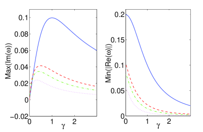
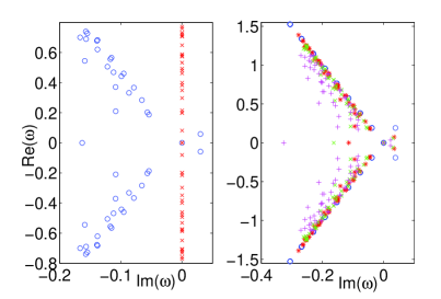
Figure 4: (Color online) Left Images: The left subpanel shows the non-vanishing imaginary part of the eigenfrequency associated with the anomalous mode, as soon as the dissipative prefactor $\gamma$ is non-zero for $\mu=0.4$, $0.8$, $1$, and $1.6$ (respective curves from top to bottom). The right subpanel is similar but now for the real part of the eigenfrequency. Here $\Omega=0.2$. Right Images: The left subpanel illustrates the linearization (so-called BdG) spectrum of the case $\gamma=0$ (red crosses) and that of $\gamma=0.2$ (blue circles) for $\mu=1$ and $\Omega=0.2$. The right subpanel shows the spectrum for $\mu=0.4$ (blue circles), $\mu=0.8$ (red stars), $\mu=1$ (green crosses) and $\mu=1.6$ (magenta pluses) for $\gamma=0.2$.

It can then be shown directly that:

$$\begin{split}\partial_{t}J(u)&=\gamma\operatorname{curl}(\partial_{t}u,\nabla u)-{1\over 2}\operatorname{curl}\operatorname{div}(\nabla u\otimes\nabla u)\\ &\quad-{1\over 2}\operatorname{curl}(|u|^{2}\nabla V),\end{split}$$ (26)

where $(a,b)={1\over 2}(ab^{*}+a^{*}b)$ is the complex inner-product and $\otimes$ denotes the tensor product.

We will now examine the magnitude of the different terms in the identity (26) by direct calculation based on an ansatz of the form $u(x,t)=\sqrt{\rho_{\rm TF}(x)}v(x-a(t))$ where $v=\sqrt{\rho}e^{i\theta}$ will denote the vortex of the homogeneous problem; in turn, the Thomas-Fermi density $\rho_{\rm TF}(x)=\mu(1-{|x|^{2}\over R^{2}_{\rm TF}})$. Then we have for the momentum term: $j(v)(x)=\rho(x)\nabla\theta(x)={1\over|x|}\rho(|x|)\tau$ where $\tau=(-y,x)/|x|$. Notice that for the spatial scales of interest to this calculation, we will have: $r=(2\mu)^{-{1\over 2}}$ with $r,|a|\ll R_{\rm TF}$, i.e., $r$ denotes a spatial scale of the order of the healing length of the vortex. In particular $\rho(r)\approx 1$. The symbol $a$ will be used to denote the vector position of the vortex, which is assumed to be well within the Thomas-Fermi radius $R_{\rm TF}$.

Integrating $J(u)$ against a spatial variable $x_{k}$ (where the subscript index $k=1,2$ denotes the two dimensions) yields

$$\int_{B_{r}(a)}x_{k}J(u)dx ={\rho^{2}(r)\over 2r}\int_{\partial B_{r}}(x_{k}+a_{k})\rho_{\rm TF}(x+a)d\ell$$

$$\quad+{1\over 2}\int_{B_{r}}\rho_{\rm TF}(x+a)\rho(|x|)\nabla\theta\times e_{k}dx.$$

Here $B_{r}(a)$ is a ball of radius $r$ around the center position $(a)$ of the vortex and $\partial B_{r}(a)$ denotes the boundary of such a region. The first among these terms yields:

$${\rho(r)\mu\over 2r}\left[2\pi ra_{k}\left[1-{r^{2}+|a|^{2}\over R_{\rm TF}^{2}}\right]-{\pi r^{3}a_{k}\over R_{\rm TF}^{2}}\right]$$

$$=\pi\rho(r)\mu a_{k}\left(1-{|a|^{2}\over R_{\rm TF}^{2}}\right)+O\left({\mu r^{2}|a|\over R_{\rm TF}^{2}}\right),$$

and the second term is found to be also of $O({\mu r^{2}|a|\over R_{\rm TF}^{2}})$. From the time derivative of the Jacobian term, we thus obtain to leading order:

$$\partial_{t}\int_{B_{r}(a)}x_{k}J(u)dx=\pi\rho(r)\mu\dot{a}.$$ (27)

A longer calculation for the moment of the dissipative term in Eq. (26) leads to an integral of the form $\int_{B_{r}(a)}x_{k}\operatorname{curl}(\partial_{t}u,\nabla u)dx$. Based on the ansatz, we get a dominant contribution of the form

$$-\gamma\mu\left[{1\over 2}\int_{B_{r}}\left|\nabla v\right|^{2}dx-\pi\rho(r)\right]\dot{a}\times e_{k}$$ (28)

with error terms bounded by $O({\mu|a|^{2}|\dot{a}|\over R_{\rm TF}^{2}})$.

The interaction term can be reshaped using the following identity: $\operatorname{curl}\operatorname{div}(\nabla u\otimes\nabla u)=\operatorname{curl}\left[(\Delta u,\nabla u)+{1\over 2}\nabla|\nabla u|^{2}\right]=\operatorname{curl}(\Delta u,\nabla u)$, and a calculation shows

$$\int_{B_{r}(a)}x_{k}\operatorname{curl}\operatorname{div}\left(\nabla u\otimes\nabla u\right)dx$$

$$\qquad=\int_{\partial B_{r}}(x_{k}+a_{k})\left(\Delta u,\partial_{\tau}u\right)d\ell$$

$$\qquad\quad+\int_{\partial B_{r}}\left(\partial_{\nu}u,\nabla u\times e_{k}\right)d\ell$$

$$\qquad\quad-\int_{\partial B_{r}}{1\over 2}\tau\cdot e_{k}\left|\nabla u\right|^{2}d\ell.$$

Using that $\int_{\partial B_{r}}(\partial_{\nu}v,\partial_{k}v)d\ell=\int_{\partial B_{r}}\tau\cdot e_{k}|\nabla v|^{2}d\ell=0$, then a similar calculation shows that in the absence of a second vortex the terms on the right hand side can be bounded by $O({\mu\over R_{\rm TF}^{2}})$.

Finally, a critical contribution is made by the potential term. If $V(x)={\Omega^{2}\over 2}|x|^{2}$ then $\partial_{j}V(x)=\Omega^{2}x_{j}$ and

$$-{1\over 2}\int_{B_{r}(a)}x_{k}\operatorname{curl}(|u(x)|^{2}\nabla V)dx$$

$$=-{\Omega^{2}\over 2}\int_{\partial B_{r}}(x_{k}+a_{k})|u(x+a)|^{2}\tau\cdot a\,d\ell$$

$$\quad-{\Omega^{2}\over 2}\int_{B_{r}}|u(x+a)|^{2}(x+a)\times e_{k}\,dx$$

which comes to

$${\Omega^{2}\over 2}\mu\left[\pi\rho(r)r^{2}-\int_{B_{r}}\rho(x)dx\right](a\times e_{k})$$ (29)

up to an error of $O({\Omega^{2}\mu|a|^{5}\over R_{\rm TF}^{2}})$.

Putting the different contributions together from Eqs (27)–(29) and dividing by $\pi\rho(r)\mu=\pi\mu$, we arrive at an effective ODE for the motion of the vortex,

$$\dot{a}+\gamma A(\dot{a}\times e_{k})=-{\Omega^{2}\over\mu}B{(a\times e_{k})},$$

where

$$A ={1\over 2\pi}\int_{B_{(2\mu)^{-{1\over 2}}}}\left|\nabla v\right|^{2}dx-1,$$

$$B ={1\over 4\pi\mu^{-1}}\int_{B_{(2\mu)^{-{1\over 2}}}}\rho(x)dx-1.$$

Since $(1-{|a|^{2}\over R_{\rm TF}^{2}})\dot{a}=\dot{a}$ up to $O({1\over R_{\rm TF}^{2}})$, we achieve the analogous ODE to the result of Eqs. (12)-(13), up to terms logarithmic in $\mu/\Omega$ and errors of $O({1\over R_{\rm TF}^{2}})$. Thus, this higher order moment method yields a similar conclusion to the one obtained by the energy methods earlier in the text. In order to discern the higher order corrections using this method, one should look at the situation when the healing length is significantly smaller than the vortex position, $r\ll|a|$.

Appendix B Stability analysis of vortices and vortex dipoles in the DGPE framework

We present here some further details related to the eigenfrequency spectrum of the single vortex and vortex dipole cases; for mathematical completeness, we present our results for values of $\gamma$ in the range $0\leq\gamma\leq 3$, noting that values of $\gamma$ well beyond the interval outlined previously (in the main text) have no physical relevance for the particular problem.

First, Fig. 4 (left plots) depicts real and imaginary parts of the eigenfrequency associated with the anomalous mode of the vortex centered at the origin for different values of $\mu$ versus $\gamma$ for the DGPE [Eq. (1)]. This shows that the mode has a positive imaginary part of the eigenfrequency (i.e., a real part of the corresponding eigenvalue, directly signaling the relevant instability) for any non-zero value of $\gamma$. In Fig. 4 (right plots), we show how the spectrum of the Hamiltonian case ($\gamma=0$) gets modified by a $\gamma\neq 0$ term depicting also the “trajectory” of the relevant eigenvalues of the spectrum for different values of the chemical potential $\mu$.

Next, turning to numerical computations based on our analytical approximations, we now examine the linearization (BdG) analysis around a single vortex (Fig. 5, left plots), as well as around a stationary VD (Fig. 5, right plots). In the former case, we observe the good agreement of our theoretical prediction of Eqs. (12)-(13) in comparison with the anomalous mode (complex) frequency associated with the single vortex spiraling outward motion; note that the real part of the relevant eigenfrequency is associated with the precession around the center, while its imaginary part with the growing radius of the relevant motion.

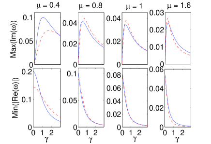
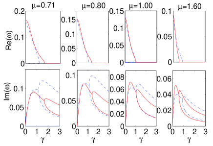
Figure 5: (Color online) Left Images: The upper four subpanels show the comparison of the imaginary (growth) part of the vortex linearization eigenfrequency associated with the anomalous mode from the BdG numerical analysis (solid blue) with the analytical results $\omega_{i}$ [see Eq. (14)] (red dashed). The lower four subpanels show the comparison of the real (oscillatory) part of the eigenfrequency associated with the anomalous mode from the BdG numerical analysis (solid blue) with the analytical results $\omega_{r}$ [see Eq. (15)] (red dashed). From the left to the right, the cases shown are for $\mu=0.4,0.8,1,1.6$, respectively, and $\Omega=0.2$. Notice the progressively improving agreement as $\mu$ increases and the Thomas-Fermi regime of vortex particle motion is reached. Right Images: Shown are the internal mode eigenfrequencies of the vortex dipole state associated with the anomalous mode from the BdG numerical analysis (dashed blue) against the dissipation term $\gamma$ for $\mu=0.71,0.80,1,1.6$ versus the analytical prediction (solid red), for $\Omega=0.2$.

As an aside, we note in passing that for sufficiently large $\gamma$ in the vortex dipole case, there is a collision of the relevant vortex pair epicyclic internal mode eigenfrequencies. This, in turn, results in the exponential expulsion of the VD constituents, a feature that is never possible to observe for isolated vortices. However, a note of caution should be added here. The values of $\gamma$ [of $O(1)$] where such phenomenology arises are roughly 3 orders of magnitude above the physically relevant values at least for the thermal damping DGPE model of BECs considered herein. Consequently, such phenomenology is simply of mathematical, rather than physical relevance.

Recall that in the case of the VD, in accordance to what was shown in Ref. middel2 , there is a pair of internal modes of the two-vortex bound state. One of these is a Goldstone mode of vanishing frequency associated with the free rotation of the pair around the trap center. However, the second mode refers to the epicyclic motion around the vortex dipole equilibrium observed in Ref. pra_11 ; this motion is also hinted at by the vortex dynamics of Ref. BPA_10 . It is the latter motion that leads to the instability (oscillatory or purely exponential, for small or large $\gamma$, respectively) observed herein. Finally, it is reassuring to note that in the dipole case, as in the single vortex case of Fig. 5, the theoretical approximation for the eigenfrequency becomes more accurate as the chemical potential $\mu$ gets larger where the vortices behave more like point particles.

References

- (1) A. L. Fetter and A. A. Svidzinsky, J. Phys. Condens. Matter 13, R135 (2001).
- (2) A. L. Fetter, Rev. Mod. Phys. 81, 647 (2009).
- (3) P. K. Newton and G. Chamoun, SIAM Rev. 51, 501 (2009).
- (4) P. G. Kevrekidis, R. Carretero-González, D. J. Frantzeskakis, and I. G. Kevrekidis, Mod. Phys. Lett. B 18 (2004) 1481–1505.
- (5) P. G. Kevrekidis, D. J. Frantzeskakis, and R. Carretero-González, Emergent Nonlinear Phenomena in Bose-Einstein Condensates: Theory and Experiment. Springer Series on Atomic, Optical, and Plasma Physics, Vol. 45 (2008).
- (6) P. K. Newton, The N-vortex problem: Analytical techniques, Springer-Verlag (New York, 2001).
- (7) L. M. Pismen, Vortices in Nonlinear Fields (Clarendon, UK, 1999).
- (8) Y. S. Kivshar, J. Christou, V. Tikhonenko, B. Luther-Davies, and L. Pismen, Opt. Comm. 152, 198 (1998).
- (9) A. Dreischuh, S. Chervenkov, D. Neshev, G. G. Paulus, and H. Walther, J. Opt. Soc. Am. B 19, 550 (2002).
- (10) K. W. Madison, F. Chevy, W. Wohlleben, and J. Dalibard, Phys. Rev. Lett. 84, 806 (2000).
- (11) S. Inouye, S. Gupta, T. Rosenband, A. P. Chikkatur, A. Görlitz, T. L. Gustavson, A. E. Leanhardt, D. E. Pritchard, and W. Ketterle, Phys. Rev. Lett. 87, 080402 (2001).
- (12) E. Hodby, G. Hechenblaikner, S. A. Hopkins, O. M. Maragò, and C. J. Foot, Phys. Rev. Lett. 88, 010405 (2001).
- (13) J. R. Abo-Shaeer, C. Raman, J. M. Vogels, and W. Ketterle, Science 292, 476 (2001).
- (14) J. R. Abo-Shaeer, C. Raman, and W. Ketterle, Phys. Rev. Lett. 88, 070409 (2002).
- (15) P. Engels, I. Coddington, P. C. Haljan, and E. A. Cornell, Phys. Rev. Lett. 89 (2002) 100403.
- (16) C. N. Weiler, T. W. Neely, D. R. Scherer, A. S. Bradley, M. J. Davis, and B. P. Anderson, Nature 455, 948 (2008).
- (17) T. W. B. Kibble, J. Phys. A 9, 1387 (1976).
- (18) W. H. Zurek, Nature 317, 505 (1985).
- (19) D. V. Freilich, D. M. Bianchi, A. M. Kaufman, T. K. Langin, and D. S. Hall, Science 320, 1182 (2010).
- (20) S. Middelkamp, P. J. Torres, P. G. Kevrekidis, D. J. Frantzeskakis, R. Carretero-González, P. Schmelcher, D. V. Freilich, and D. S. Hall Phys. Rev. A 84, 011605 (2011).
- (21) T. W. Neely, E. C. Samson, A. S. Bradley, M. J. Davis, and B. P. Anderson, Phys. Rev. Lett. 104, 160401 (2010).
- (22) J. A. Seman, E. A. L. Henn, M. Haque, R. F. Shiozaki, E. R. F. Ramos, M. Caracanhas, P. Castilho, C. Castelo Branco, P. E. S. Tavares, F. J. Poveda-Cuevas, G. Roati, K. M. F. Magalhaes, and V. S. Bagnato Phys. Rev. A 82, 033616 (2010).
- (23) R. Navarro, R. Carretero-González, P. J. Torres, P. G. Kevrekidis, D. J. Frantzeskakis, M. W. Ray, E. Altuntaş, and D. S. Hall, Phys. Rev. Lett. 110, 225301 (2013).
- (24) N. P. Proukakis, S. A. Gardiner, M. J. Davis, and M. H. Szymanska (Eds.), Quantum Gases: Finite Temperature and Non-Equilibrium Dynamics (Imperial College Press, London, 2013).
- (25) P. O. Fedichev, A. E. Muryshev, and G. V. Shlyapnikov, Phys. Rev. A 60, 3220 (1999).
- (26) A. Muryshev, G. V. Shlyapnikov, W. Ertmer, K. Sengstock, and M. Lewenstein, Phys. Rev. Lett. 89, 110401 (2002).
- (27) S. P. Cockburn, H. E. Nistazakis, T. P. Horikis, P. G. Kevrekidis, N. P. Proukakis, and D. J. Frantzeskakis, Phys. Rev. Lett. 104, 174101 (2010); ibid. Phys. Rev. A 84, 043640 (2011).
- (28) N. P. Proukakis, N. G. Parker, C. F. Barenghi, and C. S. Adams, Phys. Rev. Lett. 93, 130408 (2004).
- (29) B. Jackson, N. P. Proukakis, and C. F. Barenghi, Phys, Rev. A 75, 051601 (2007); B. Jackson, C. F. Barenghi, and N. P. Proukakis, J. Low Temp. Phys. 148, 387 (2007);
- (30) W. H. Zurek, Phys. Rev. Lett. 102, 105702 (2009); B. Damski, and W. H. Zurek, Phys. Rev. Lett. 104, 160404 (2010).
- (31) A. D. Martin and J. Ruostekoski, Phys. Rev. Lett. 104, 194102 (2010); A. D. Martin and J. Ruostekoski, New J. Phys. 12, 055018 (2010).
- (32) D. M. Gangardt and A. Kamenev, Phys. Rev. Lett. 104, 190402 (2010).
- (33) K. J. Wright and A. S. Bradley, arXiv:1104.2691.
- (34) S. Burger, K. Bongs, S. Dettmer, W. Ertmer, K. Sengstock, A. Sanpera, G. V. Shlyapnikov, and M. Lewenstein, Phys. Rev. Lett. 83, 5198 (1999).
- (35) K. Bongs, S. Burger, S. Dettmer, D. Hellweg, J. Arlt, W. Ertmer, and K. Sengstock, C. R. Acad. Sci. Paris 2, 671 (2001).
- (36) J. Denschlag, J. E. Simsarian, D. L. Feder, C. W. Clark, L. A. Collins, J. Cubizolles, L. Deng, E. W. Hagley, K. Helmerson, W. P. Reinhardt, S. L. Rolston, B. I. Schneider, and W. D. Phillips, Science 287, 97 (2000).
- (37) C. Becker, S. Stellmer, P. Soltan-Panahi, S. Dörscher, M. Baumert, E. M. Richter, J. Kronjäger, K. Bongs, and K. Sengstock, Nature Physics 4, 496 (2008); S. Stellmer, C. Becker, P. Soltan-Panahi, E. M. Richter, S. Dörscher, M. Baumert, J. Kronjäger, K. Bongs, and K. Sengstock, Phys. Rev. Lett. 101, 120406 (2008)
- (38) A. Weller, J. P. Ronzheimer, C. Gross, J. Esteve, M. K. Oberthaler, D. J. Frantzeskakis, G. Theocharis, and P. G. Kevrekidis, Phys. Rev. Lett. 101, 130401 (2008); G. Theocharis, A. Weller, J. P. Ronzheimer, C. Gross, M. K. Oberthaler, P. G. Kevrekidis, and D. J. Frantzeskakis, Phys. Rev. A, 81, 063604 (2010)
- (39) Th. Busch and J. R. Anglin Phys. Rev. Lett. 84, 2298 (2000).
- (40) G. Theocharis, P. G. Kevrekidis, M. K. Oberthaler, and D. J. Frantzeskakis, Phys. Rev. A 76, 045601 (2007).
- (41) T. Yefsah, A. T. Sommer, M. J. H. Ku, L. W. Cheuk, W. J. Ji, W. S. Bakr, and M. W. Zwierlein, Nature 499, 426 (2013)
- (42) D. J. Frantzeskakis, J. Phys. A: Math. Theor. 43, 213001 (2010).
- (43) L. P. Pitaevskii, Zh. Eksp. Teor. Fiz. 35, 408 (1958) [Sov. Phys. JETP 35, 282 (1959)].
- (44) A. A. Penckwitt, R. J. Ballagh, and C. W. Gardiner, Phys. Rev. Lett. 89, 260402 (2002).
- (45) B. Jackson and N. P. Proukakis, J. Phys. B: At. Mol. Opt. Phys. 41, 203002 (2008).
- (46) P. B. Blakie, A. S. Bradley, M. J. Davis, R. J. Ballagh, and C. W. Gardiner, Adv. Phys. 57, 363 (2008).
- (47) A. Griffin, T. Nikuni, and E. Zaremba, Bose-Condensed Gases at Finite Temperatures (Cambridge University Press, Cambridge, 2009).
- (48) H. T. C. Stoof, J. Low Temp. Phys. 114, 11 (1999); H. T. C. Stoof, and M. J. Bijlsma, J. Low Temp. Phys 124, 431 (2001).
- (49) S. P. Cockburn and N. P. Proukakis, Laser Phys. 19, 558 (2009).
- (50) P. G. Kevrekidis and D. J. Frantzeskakis, Discr. Cont. Dyn. Sys. S 4, 1199 (2011).
- (51) V Achilleos, D Yan, P G Kevrekidis, and D J Frantzeskakis, New J. Phys. 14, 055006 (2012).
- (52) B. Jackson, N. P. Proukakis, C. F. Barenghi, and E. Zaremba, Phys. Rev. A 79, 053615 (2009).
- (53) A. J. Allen, E. Zaremba, C. F. Barenghi, N. P. Proukakis, Phys. Rev. A 87, 013630 (2013).
- (54) S. Middelkamp, P. G. Kevrekidis, D. J. Frantzeskakis, R. Carretero-González, P. Schmelcher J. Phys. B 43, 155303 (2010).
- (55) S. J. Rooney, A. S. Bradley, and P. B. Blakie Phys. Rev. A 81, 023630 (2010).
- (56) T. M. Wright, A. S. Bradley, and R. J. Ballagh, Phys. Rev. A 80, 053624 (2009)
- (57) M. Kurzke, C. Melcher, R. Moser, and D. Spirn, Indiana Univ. J. Math. 58, 2597 (2009).
- (58) E. Moit, Anal. PDE 2, 159 (2009)
- (59) L. Thompson and P. C. E. Stamp, Phys. Rev. Lett. 108, 184501 (2012); T. Cox and P. C. E. Stamp, arXiv:1207.4237 [cond-mat.quant-gas]
- (60) R. A. Duine, B. W. A. Leurs, and H. T. C. Stoof, Phys. Rev. A 69, 053623 (2004).
- (61) A. S. Bradley, C. W. Gardiner, http://xxx.lanl.gov/abs/cond-mat/0509592.
- (62) D. E. Pelinovsky and P. G. Kevrekidis Nonlinearity 24, 1271 (2011); see also for the case of dark solitons M. P. Coles, D. E. Pelinovsky, and P. G. Kevrekidis Nonlinearity 23, 1753 (2010).
- (63) As this model is of broader mathematical interest, for completeness, our analysis in Appendix B also extends beyond this regime, even if not directly relevant to cold atoms.
- (64) T. Kapitula, P. G. Kevrekidis, and B. Sandstede, Phys. D 195, 263 (2004).
- (65) E. Lundh and P. Ao, Phys. Rev. A 61, 063612 (2000).
- (66) N. G. Berloff, J. Phys. A 37, 1617 (2004).
- (67) In a very recent work, the motion of a single vortex and of a vortex dipole was explored numerically in the framework of the stochastic GPE in S. Gautam et al, arXiv:1309.6205.
- (68) R. L. Jerrard and D. Smets, arXiv:1301.5213.
- (69) S. McEndoo and Th. Busch Phys. Rev. A 79, 053616 (2009).
- (70) S. Middelkamp, P. G. Kevrekidis, D. J. Frantzeskakis, R. Carretero-González, and P. Schmelcher Phys. Rev. A 82, 013646 (2010).
- (71) N. G. Parker, A. J. Allen, C. F. Barenghi, and N. P. Proukakis, Phys. Rev. A 86, 013631 (2012).
- (72) A. J. Allen, D. P. Jackson, C. F. Barenghi, and N. P. Proukakis, Phys. Rev. A 83, 013613 (2011).
- (73) It should be noted that in this case the condensate is sufficiently wide that the homogeneous case value of has been utilized.
- (74) B. P. Anderson, P. C. Haljan, C. A. Regal, D. L. Feder, L. A. Collins, C. W. Clark, and E. A. Cornell, Phys. Rev. Lett. 86, 2926 (2001).
- (75) N. S. Ginsberg, J. Brand, and L. V. Hau, Phys. Rev. Lett. 94, 040403 (2005).
- (76) S. Komineas, Eur. Phys. J. Spec. Top. 147, 133 (2007).