A Holographic Path to the Turbulent Side of Gravity

Abstract

We study the dynamics of a $2+1$ dimensional relativistic viscous conformal fluid in Minkowski spacetime. Such fluid solutions arise as duals, under the “gravity/fluid correspondence”, to $3+1$ dimensional asymptotically anti-de Sitter (AAdS) black brane solutions to the Einstein equation. We examine stability properties of shear flows, which correspond to hydrodynamic quasinormal modes of the black brane. We find that, for sufficiently high Reynolds number, the solution undergoes an inverse turbulent cascade to long wavelength modes. We then map this fluid solution, via the gravity/fluid duality, into a bulk metric. This suggests a new and interesting feature of the behavior of perturbed AAdS black holes and black branes, which is not readily captured by a standard quasinormal mode analysis. Namely, for sufficiently large perturbed black objects (with long-lived quasinormal modes), nonlinear effects transfer energy from short to long wavelength modes via a turbulent cascade within the metric perturbation. As long wavelength modes have slower decay, this lengthens the overall lifetime of the perturbation. We also discuss various implications of this behavior, including expectations for higher dimensions, and the possibility of predicting turbulence in more general gravitational scenarios.

I Introduction

The AdS/CFT correspondence Maldacena (1998); Aharony et al. (2000) proposes a remarkable connection between quantum gravity in $d+1$ dimensions and quantum field theory in $d$ dimensions. In a certain classical limit, this correspondence can be utilized to link the behavior of perturbed asymptotically anti-de Sitter (AAdS) black branes in general relativity to that of viscous conformal fluids on the AdS boundary, provided the perturbations are of sufficiently long wavelength Baier et al. (2008); Bhattacharyya et al. (2008a, b); Van Raamsdonk (2008). This limit of the AdS/CFT correspondence is known as the gravity/fluid correspondence.

The gravity/fluid correspondence can also be derived on its own in a purely classical manner without any appeal to AdS/CFT, as a derivative expansion within general relativity (see, e.g., Ref. Bhattacharyya et al. (2008a)). This derivation provides an explicit perturbative mapping between solutions, which can be exploited to relate gravitational and fluid behavior. In particular, interesting known phenomena on one side of the duality should have counterparts on the other, which can lead to new predictions, or to new methods of analysis. This has been used as a means to frame fluid dynamics questions in terms of gravitational physics. For example, Ref. Oz and Rabinovich (2011) explored the relation between the Penrose inequalities – which predict the onset of naked singularities in general relativity – and finite-time blowup of solutions in hydrodynamics. In Ref. Eling et al. (2010), it was suggested that a gravity dual could be utilized to understand the complex phenomenon of fluid turbulence. In the present work, following the analysis presented in Ref. Carrasco et al. (2012), we follow the opposite route, namely to study the implications that turbulent phenomena – that can arise in fluid dynamics – have for our understanding of general relativity.

Turbulence is a ubiquitous property of fluid flows observed in nature at sufficiently high Reynolds number, $R$. Such behavior has recently been shown to also arise in inviscid conformal relativistic hydrodynamics Carrasco et al. (2012); Radice and Rezzolla (2013). While the actual fluid dual to an AAdS black brane has nonzero shear viscosity, this viscosity is subleading in the black hole temperature, so the inviscid approximation is valid at sufficiently high temperature Carrasco et al. (2012). This suggests that there should be a corresponding regime where long-wavelength black hole perturbations in asymptotically AdS spacetimes behave in a turbulent manner. Furthermore, in $2+1$ dimensions such inviscid conformal fluids display an inverse cascade of energy to large scales Carrasco et al. (2012), in accord with intuition from Navier-Stokes fluids Kraichnan (1967). This ensures that provided the initial condition falls within the regime of applicability of the gravity/fluid correspondence (i.e., sufficiently long wavelength perturbations), so should its time evolution, and therefore there should exist a black brane that behaves in a dual manner. The intuition described here has been borne out in very recent ground-breaking work Adams et al. (2013), which demonstrated the development of turbulence in gravitational perturbations in $3+1$ spacetime dimensions. Thus, gravitational behavior in this regime is effectively captured by a hydrodynamic analysis.

Drawing again on intuition from fluids, one should also expect on the gravity side, behavior akin both to turbulent and laminar flow. It is important to emphasize that these two phenomena can arise on the fluid side irrespective of the velocity of the background flow alone. Rather, the behavior depends on the value of the Reynolds number,

$$R\sim\frac{\rho vL}{\eta},$$ (1)

where $\rho$, $v$, $L$, and $\eta$ are the characteristic energy density, velocity fluctuation, distance scale, and shear viscosity, describing the flow, respectively. For high values of $R$, turbulence occurs, whereas for small values the flow is laminar.

These results and observations concerning the turbulent nature of perturbed AAdS black branes appear to be in tension with the standard expectation that such perturbations decay exponentially via quasinormal modes Berti et al. (2009); Morgan et al. (2009). Indeed, for small-amplitude gravitational perturbations (which are dual to fluid flows with small velocity fluctuations $v$), a linear analysis should be valid. Due to the symmetries of the black brane, a mode decomposition is then possible. Such an analysis indicates that the modes decay in time as radiation is absorbed by the black brane (the only place where energy is lost, as the AdS boundary acts a mirror). Quasinormal modes of black branes in AdS can be grouped into three “channels” based upon their transformation properties under rotations: the sound, shear, and scalar channels. The longest lived families of modes within the sound and shear channels, in turn, are known as the “hydrodynamic” quasinormal modes of the black brane Kovtun and Starinets (2005). The dual fluid captures the behavior associated with these quasinormal modes. (Of course, the fluid satisfies nonlinear equations, whereas quasinormal modes are solutions to linear equations.) Higher quasinormal modes decay more rapidly, and are neglected in the gravity/fluid correspondence.

Of course, any behavior dual to quasinormal mode decay is surely absent in analyses of fluids with vanishing viscosity. In this paper, in order to examine this issue more closely, we extend the previous analysis of Ref. Carrasco et al. (2012) to include viscosity, which captures the role of the black brane as a sink of energy. We numerically study turbulent (and laminar) solutions for the viscous relativistic conformal fluid (in $d=2+1$) which arises in the gravity/fluid correspondence. We then contrast our results with the expectations we have laid out for the gravity dual, and we draw conclusions about the regime of applicability of linear perturbation theory about black holes.

In the following section we review the gravity/fluid correspondence in more detail. We sketch the perturbative derivation from general relativity, and we write down the relevant equations for our work. The dissipative relativistic hydrodynamic equations are closely related to those of Israel and Stewart Israel (1976); Israel and Stewart (1976, 1979), and are thus suitable for numerical implementation Baier et al. (2008). In Sec. III we proceed to describe our numerical setup, as well as the initial data. We work in Minkowski spacetime on $\mathbb{R}\times T^{2}$, which is dual to a (periodically identified) black brane in a Poincaré patch of AdS. Our initial data consists of a shear flow, which corresponds on the gravity side to a hydrodynamic shear quasinormal mode of the black brane. Due to the presence of viscosity, the shear flow is expected to decay exponentially in the absence of turbulence, until the fluid reaches an equilibrium state, corresponding to a (uniformly boosted) black brane.

We present our results in Sec. IV. Our simulations confirm that turbulent behavior and the inverse cascade continue to manifest beyond a critical Reynolds number $R_{c}$, which we determine numerically. For $R>R_{c}$, the background decaying shear flow is linearly unstable to perturbations. Such perturbations can grow until they reach the amplitude of the background shear flow, at which point fully developed turbulence is attained. As in the inviscid case Carrasco et al. (2012), an inverse cascade of energy is observed, eventually leaving two large counter-rotating vortices. On the other hand, for $R<R_{c}$, the shear flow is stable to perturbations, and it decays exponentially.

Finally, in Sec. V (as well as Appendices A and B) we use the gravity/fluid correspondence to relate our results for the fluid to the AAdS black brane. The case of laminar shear flow corresponds directly to the ordinary decay of the hydrodynamic shear quasinormal mode of the black brane. However, for $R>R_{c}$, the instability of the fluid flow corresponds to an instability of the quasinormal mode. (We stress that this does not imply an instability of the black brane, since an overall decay continues to occur.) Once the growing mode becomes of order the original quasinormal mode, the original decay is interrupted and the overall behavior is strongly modified by a fully developed turbulent behavior. In the 4-dimensional bulk, the energy cascades to the longest wavelength that fits within our torus.

We conclude that ordinary perturbation theory about the uniform black brane background is not the most suitable method of analysis for capturing such effects analytically. In fact, the instability is only clearly apparent if one linearizes the Einstein equation about the decaying quasinormal mode solution itself. (Perturbation theory about the uniform black brane would have to be implemented to higher orders before the exponential growth could be recognized.) Physically, the reason for this behavior is that, for high-temperature black branes in AdS, the lowest lying quasinormal modes become very long lived. Thus, for a given perturbation, as the temperature is increased, the linear viscous damping term becomes small compared with nonlinear terms in the Einstein equation. The regime of applicability of linear perturbation theory is thus pushed to very small metric perturbations. On the fluid side, such properties are conveniently captured by the Reynolds number (although, as noted above, a relativistic generalization is desirable for relativistic fluids). Thus it would be very interesting to obtain a geometrical realization of the Reynolds number, in order to predict the onset of turbulence in gravity Evslin (2012).

More generally, the unstable nature of certain long-lived quasinormal modes suggests that the decay of a sufficiently perturbed black brane can deviate from the picture suggested by ordinary perturbation theory. Rather than being describable by quasinormal decay, the black brane can undergo a turbulent cascade with a power law decay. Only after the energy cascades to long wavelengths will a quasinormal mode decay take hold.

In this work, we follow all notation and sign conventions of Wald (1984). We use lower case Greek letters $(\mu,\nu=0,1,\ldots,d-1)$ for indices of boundary quantities, and we upper case Latin letters $(M,N=0,1,\ldots,d)$ in the bulk. Boundary indices are raised and lowered with the boundary Minkowski metric $\eta_{\mu\nu}$.

II Gravity/Fluid Correspondence

In this section we review the basic results of the gravity/fluid correspondence. We sketch the derivation from Einstein’s equation in the bulk. We also discuss issues concerning the well-posedness of viscous relativistic fluids, and we write down suitable equations of motion that will be used in our simulations Baier et al. (2008). The derivation which we review below follows that of Bhattacharyya et al Bhattacharyya et al. (2008a).

As noted in the introduction, we restrict to boundary fluids in Minkowski spacetime, which are dual to perturbed AAdS black branes. Our simulations adopt $d=3$, but in this section we keep $d$ arbitrary. We also take the boundary manifold to be $\mathbb{R}\times T^{2}$; that is, we impose periodic boundary conditions along boundary spatial directions. Results in $d=3$ were derived in Ref. Van Raamsdonk (2008), while the arbitrary $d$ case whose equations we write down was analyzed in Refs. Haack and Yarom (2008); Bhattacharyya et al. (2008b).

The starting point for the derivation of the gravity/fluid correspondence is a uniform boosted black brane spacetime, which, written in ingoing Eddington-Finkelstein coordinates, reads,

$$ds^{2}_{[0]}=-2u_{\mu}dx^{\mu}dr+r^{2}\left(\eta_{\mu\nu}+\frac{1}{(br)^{d}}u_{\mu}u_{\nu}\right)dx^{\mu}dx^{\nu}.$$ (2)

Here, the fields $b$ and $u_{\mu}$ (satisfying $u^{\mu}u_{\mu}=-1$) are constants. This is a solution to the bulk Einstein equation,

$$G_{AB}+\Lambda g_{AB}=0,$$ (3)

with the cosmological constant $\Lambda=-d(d-1)/2$. The boosted black brane is related to the static black brane by a coordinate transformation. The coordinates $x^{\mu}=(t,x,y)$ are to be thought of as “boundary” coordinates, while the coordinate $r$ is the “bulk” radial coordinate.

To each asymptotically AdS bulk solution, is associated a metric and conserved stress-energy tensor on the timelike boundary of the spacetime at $r\to\infty$ (see, e.g., Ref. Balasubramanian and Kraus (1999) or Appendix A for the precise definition). The boundary metric, in the case of (2) is $\eta_{\mu\nu}$, while the boundary stress-energy tensor is

$$T_{\mu\nu}^{[0]}=\frac{1}{16\pi G_{d+1}b^{d}}(du_{\mu}u_{\nu}+\eta_{\mu\nu}).$$ (4)

This is a fluid stress-energy tensor, so one may read off the energy density and pressure,

$$\rho =\frac{d-1}{16\pi G_{d+1}b^{d}},$$ (5)

$$P =\frac{1}{16\pi G_{d+1}b^{d}}.$$ (6)

The stress-energy tensor is traceless, with equation of state

$$P=\frac{\rho}{d-1},$$ (7)

as required by conformal invariance. Imposing the first law of thermodynamics, $\mathrm{d}\rho=T\mathrm{d}s$, as well as the relation $\rho+P=sT$, gives the entropy density $s$ and fluid temperature $T$,

$$s =AT^{d-1},$$ (8)

$$\rho =\frac{d-1}{d}AT^{d}.$$ (9)

Here, $A$ is a constant of integration. This is fixed to $A\equiv(4\pi)^{d}/(16\pi G_{d+1}d^{d-1})$ by equating $T$ with the Hawking temperature $T_{Hawking}=d/(4\pi b)$ of the black brane.

To move beyond the uniform fluid, $b$ and $u_{\mu}$ are promoted to functions of the boundary coordinates $x^{\mu}$, which are slowly varying; that is, if $L$ is the length scale of variation of these fields, then $L\gg b$. At this point, the metric (2) is no longer a solution to Einstein’s equation. However, due to the fact that the fields are slowly varying, it is possible to systematically correct the metric order by order in a derivative expansion, so that Einstein’s equation is solved to any given order in derivatives. One can then compute the boundary stress-energy tensor corresponding to the metric at each order, and take this as defining the boundary fluid.

In this setup, the boundary metric is fixed to $\eta_{\mu\nu}$ throughout. This can be thought of as a “Dirichlet condition” on the boundary. The Einstein equation reduces to a set of “constraints” along the timelike boundary of AdS, as well as evolution equations into the bulk. The “momentum constraint” gives rise to conservation of boundary stress-energy, while the “Hamiltonian constraint” ensures tracelessness. The “evolution equations” reduce to ordinary differential equations along $r$. Regularity at the future black brane horizon is imposed as one of the boundary conditions for these ODEs. This corresponds to the imposition of an ingoing boundary condition, and it is responsible for the breaking of time-reversal symmetry inherent in the fluid viscosity term. The “Landau frame” gauge condition,

$$u^{\nu}T_{\mu\nu}\propto u_{\mu},$$ (10)

is also imposed.

After a rather long, but direct, calculation, the resulting boundary stress-energy tensor – to second order in derivatives – is found to be

$$T_{\mu\nu}^{[0+1+2]}=\frac{\rho}{d-1}\left(du_{\mu}u_{\nu}+\eta_{\mu\nu}\right)+\Pi_{\mu\nu},$$ (11)

where the viscous part, $\Pi_{\mu\nu}$, is (see Eq. (3.11) of Ref. Baier et al. (2008), Eq. (1.5) of Ref. Haack and Yarom (2008), or Eq. (1.3) of Ref. Bhattacharyya et al. (2008b))

$$\Pi_{\mu\nu}={} -2\eta\sigma_{\mu\nu}$$

$$+2\eta\tau_{\Pi}\left(\langle u^{\alpha}\partial_{\alpha}\sigma_{\mu\nu}\rangle+\frac{1}{d-1}\sigma_{\mu\nu}\partial_{\alpha}u^{\alpha}\right)+\langle\lambda_{1}\sigma_{\mu\alpha}\sigma_{\nu}^{\phantom{\nu}\alpha}+\lambda_{2}\sigma_{\mu\alpha}\omega_{\nu}^{\phantom{\nu}\alpha}+\lambda_{3}\omega_{\mu\alpha}\omega_{\nu}^{\phantom{\nu}\alpha}\rangle.$$ (12)

The shear and vorticity tensors are given by

$$\sigma_{\mu\nu} \equiv\langle\partial_{\mu}u_{\nu}\rangle,$$ (13)

$$\omega_{\mu\nu} \equiv P_{\mu}^{\phantom{\mu}\alpha}P_{\nu}^{\phantom{\nu}\beta}\partial_{[\alpha}u_{\beta]}.$$ (14)

The angled brackets denote the symmetric traceless part of the projection orthogonal to $u^{\mu}$,

$$\langle A_{\mu\nu}\rangle\equiv\left(P_{(\mu}^{\phantom{(\mu}\alpha}P_{\nu)}^{\phantom{\nu)}\beta}-\frac{1}{d-1}P_{\mu\nu}P^{\alpha\beta}\right)A_{\alpha\beta},$$ (15)

while $P_{\mu\nu}$ is the spatial projector orthogonal to $u^{\mu}$,

$$P_{\mu\nu}\equiv\eta_{\mu\nu}+u_{\mu}u_{\nu}.$$ (16)

It may be verified that $\Pi_{\mu\nu}$ is symmetric and satisfies

$$\Pi^{\mu}_{\phantom{\mu}\mu} =0,$$ (17)

$$u^{\nu}\Pi_{\mu\nu} =0.$$ (18)

The transport coefficients $\{\eta,\,\tau_{\Pi},\,\lambda_{i}\}$ have been worked out explicitly in various dimensions Van Raamsdonk (2008); Haack and Yarom (2008); Bhattacharyya et al. (2008b),

$$\eta =\frac{s}{4\pi},$$ (19)

$$\tau_{\Pi} =b\left[1-\int_{1}^{\infty}\frac{y^{d-2}-1}{y(y^{d}-1)}\,\mathrm{d}y\right]\xrightarrow{d=3}b\left(1-\frac{1}{2}\log 3+\frac{\pi}{6\sqrt{3}}\right),$$ (20)

$$\lambda_{1} =\frac{\eta b}{2},$$ (21)

$$\lambda_{2} =-2\eta b\int_{1}^{\infty}\frac{y^{d-2}-1}{y(y^{d}-1)}\,\mathrm{d}y\xrightarrow{d=3}-\eta b\left(\log 3-\frac{\pi}{3\sqrt{3}}\right),$$ (22)

$$\lambda_{3} =0.$$ (23)

Thus, the boundary fluid has a nonzero shear viscosity $\eta$, but the bulk viscosity vanishes, so that the stress-energy tensor remains traceless. Conformal invariance can also be used to deduce the presence of the particular nonzero second order transport coefficients directly Baier et al. (2008). For completeness, we note that conservation of the boundary stress-energy tensor leads to the equations of motion for $\rho$ and $u^{\mu}$,

$$0 =u^{\mu}\partial_{\mu}\rho+\frac{d}{d-1}\rho\partial_{\mu}u^{\mu}-u^{\mu}\partial^{\nu}\Pi_{\mu\nu},$$ (24)

$$0 =\frac{d}{d-1}\rho u^{\mu}\partial_{\mu}u^{\alpha}+\frac{1}{d-1}\partial^{\alpha}\rho-\frac{d}{(d-1)^{2}}u^{\alpha}\rho\partial_{\mu}u^{\mu}+\frac{1}{d-1}u^{\alpha}u^{\mu}\partial^{\nu}\Pi_{\mu\nu}+P^{\alpha\mu}\partial^{\nu}\Pi_{\mu\nu}.$$ (25)

It is easy to see that in this derivative expansion, $\Pi_{\mu\nu}$ is subleading in $b/L$, as compared with the perfect fluid stress-energy tensor $T_{\mu\nu}^{(0)}$. Thus, given a fixed $L$, the viscous part may be neglected for small $b$, or, equivalently, large $T$. This is the limit which was taken in Ref. Carrasco et al. (2012). In this work, however, we wish to move beyond the $T\to\infty$ limit, so viscosity must be included in our simulations. As explained in the introduction, this corresponds on the gravity side to the effects of energy losses through the horizon.

At this point, one may wonder why we have bothered to include terms to second order in derivatives, since the shear viscosity appears at first order. The reason is that relativistic viscous fluid formulations which are first order in derivatives, as originally laid out by Eckart Eckart (1940), lead to acausal propagation, and are generally ill-posed Israel (1976). It turns out to be possible to resolve these issues and to produce a hyperbolic system by including second order terms; in particular, the term involving $\tau_{\Pi}$ Israel and Stewart (1976); Israel (1976); Israel and Stewart (1979); Hiscock and Lindblom (1983). The second order terms which appear in Eq. (II) resolve the problems introduced by the viscosity, but they bring about analogous issues at higher order. To fully resolve these difficulties, it is necessary to promote $\Pi_{\mu\nu}$ to an independent field. Then, one reduces the order of the system of equations by substituting $-2\eta\sigma_{\mu\nu}\to\Pi_{\mu\nu}$ on the second line of (II). This substitution is consistent to the order to which we are working in the derivative expansion. Furthermore, this assumption will remain valid in $2+1$ dimensions under time evolution by virtue of the expected inverse cascade Carrasco et al. (2012). Therefore, following Baier et al Baier et al. (2008), we obtain

$$\Pi_{\mu\nu}={} -2\eta\sigma_{\mu\nu}$$

$$-\tau_{\Pi}\left(\langle u^{\alpha}\partial_{\alpha}\Pi_{\mu\nu}\rangle+\frac{d}{d-1}\Pi_{\mu\nu}\partial_{\alpha}u^{\alpha}\right)+\langle\frac{\lambda_{1}}{\eta^{2}}\Pi_{\mu\alpha}\Pi_{\nu}^{\phantom{\nu}\alpha}-\frac{\lambda_{2}}{\eta}\Pi_{\mu\alpha}\omega_{\nu}^{\phantom{\nu}\alpha}+\lambda_{3}\omega_{\mu\alpha}\omega_{\nu}^{\phantom{\nu}\alpha}\rangle.$$ (26)

The formulation we have described above also includes additional second order terms with coefficients $\{\lambda_{i}\}$. We have decided to include these in the interest of completeness, although we find that they have no effect on our results. Indeed, as discussed by Geroch Geroch (1995, 2001), all hyperbolic relativistic theories of fluids with viscosity should be physically equivalent. By this, one means that any additional terms in the equations of motion, when evaluated within the domain of applicability of the theory, should be small, as compared with the lower order terms. That is, if the higher order terms became important, then there would be no justification in not including even higher order terms, and the perturbative expansion would break down. This also means that the specific value of $\tau_{\Pi}$ is unimportant, so long as it is sufficiently large that the theory is causal. (We will use this fact later to increase its value in order to speed up our numerical simulations.)

To summarize, the system of interest is described by Eqs. (24), (25), and (II). These equations, however, require further manipulation prior to numerical implementation. For comparison, we recall that in the context of inviscid hydrodynamics, it is covenient to express the hydrodynamic equations in conservation form (see, e.g., LeVeque (2002)). That is, $t$-derivatives of energy and momentum density are equated with $x^{i}$-derivatives of fluxes. Such a form of the equations is particularly advantageous when studying solutions that can develop sharp gradients or discontinuities, and was employed in Ref. Carrasco et al. (2012). However, a simple extension of this approach is not possible in the presence of viscosity since the evolution equation (II) for $\Pi_{\mu\nu}$ is not of the desired form. In particular, since $P_{\mu\nu}$ projects orthogonally to $u^{\mu}$ rather than to $\partial_{t}^{\mu}$, this equation contains a $t$-derivative of $u^{\mu}$ in addition to that of $\Pi_{\mu\nu}$. However, since the presence of viscocity prevents the development of steep gradients and discontinuities in our solutions, adopting a conservative form is not necessary.

We therefore follow an approach similar to that employed in Luzum and Romatschke (2008); Romatschke (2010) within the context of heavy ion collisions. To begin, we note that in $d=3$ the conditions $u_{\mu}u^{\mu}=-1$, $u^{\nu}\Pi_{\mu\nu}=0$, and $\Pi^{\mu}_{\phantom{\mu}\mu}=0$ reduce the number of dynamical variables to five. We take these to be $\mathcal{U}\equiv(\rho,u_{x},u_{y},\Pi_{xx},\Pi_{xy})$. Equations (24), (25), and (II) are quite complicated when expressed in terms of $\mathcal{U}$, and in order to evolve the equations numerically, one must solve for the $t$-derivatives of the fields. Using computational algebra software, we can write our equations in the desired form,

$$\partial_{t}\mathcal{U}=\mathcal{F}(\mathcal{U},\partial_{i}\mathcal{U});$$ (27)

and these are the equations we implement in our code.

III Simulations

In this section we describe our choice of initial data and details of our numerical setup.

III.1 Initial data

As described in the introduction, we choose initial data corresponding to a shear hydrodynamic quasinormal mode of the black brane. Our studies concentrate on nonlinear phenomena described by the system; however, for future reference, in this subsection we analyse the evolution under the linearized equations of motion.

Consider perturbations about a uniform fluid solution,

$$\rho_{(0)} =\text{constant},$$ (28)

$$u_{(0)}^{\mu} =(1,0,0),$$ (29)

$$\Pi^{(0)}_{\mu\nu} =0,$$ (30)

which is dual to a non-boosted uniform black brane in the bulk. Solutions to the linearized equations of motion whose only nonzero perturbed fields are $u_{(1)}^{x}=u_{(1)}^{x}(t,y)$ and $\Pi^{(1)}_{xy}=\Pi^{(1)}_{yx}=\Pi^{(1)}_{xy}(t,y)$ describe shear flow. That is, fluid flow orthogonal to the velocity gradient Baier et al. (2008). The linearized equations of motion for shear flow reduce to

$$0 =\frac{3}{2}\rho_{(0)}\partial_{t}u^{x}_{(1)}+\partial_{y}\Pi^{(1)}_{xy},$$ (31)

$$\Pi_{xy} =-\eta_{(0)}\partial_{y}u_{x}^{(1)}-\tau_{\Pi}^{(0)}\partial_{t}\Pi^{(1)}_{xy},$$ (32)

which may be solved by expanding in Fourier modes. Considering one mode, with spacetime dependence the form $\sim e^{-i\omega t+iky}$, Eqs. (31) and (32) give Baier et al. (2008)

$$0=\omega^{2}+\frac{i}{\tau_{\Pi}^{(0)}}\omega-\frac{2k^{2}\eta_{(0)}}{3\rho_{(0)}\tau_{\Pi}^{(0)}}.$$ (33)

This has two solutions for small $k$,

$$\omega_{1}\approx-i\frac{2k^{2}\eta_{(0)}}{3\rho_{(0)}}=-i\frac{k^{2}}{4\pi T_{(0)}},\qquad\omega_{2}\approx-\frac{i}{\tau_{\Pi}^{(0)}},$$ (34)

both of which describe pure exponential decay. The first solution corresponds, in the bulk, to the hydrodynamic shear quasinormal mode of the black brane Baier et al. (2008); Bhattacharyya et al. (2008a); Kovtun and Starinets (2005). (The second solution shows that $\tau_{\Pi}$ is the decay timescale for $\Pi_{\mu\nu}$ to approach $-2\eta\sigma_{\mu\nu}$.)

Thus, since we are interested in understanding the corresponding black brane quasinormal mode in a nonlinear context, we choose initial data with

$$\rho(t=0) =\rho_{0}=\text{constant},$$ (35)

$$u_{x}(t=0) =v_{0}\sin\left(\frac{2\pi ny}{D}\right),$$ (36)

and all other fields zero. We vary the background energy density $\rho_{0}$, velocity amplitude $v_{0}$, the number of modes $n$, and the torus size $[0,D]^{2}$. The reason $n$ and $D$ are varied separately (rather than as the wavelength $\lambda=D/n$) is that effects due to the finite size of the box can come into play for small $n$.

Moving from the linear to nonlinear level, we expect the pure decay of this shear flow to persist, at least for small velocities. That this is the case will be verified in Sec. IV. We also keep the velocities small in most of our simulations in order to match to the linear predictions.

Our main reason for setting up this flow, of course, is to study its stability. In order to do so, we also initially seed $u_{x}$ with a very small random perturbation. By studying the effects of this perturbation, one can learn about the robustness (or lack thereof) of pure quasinormal mode decay.

III.2 Numerical setup

Equation (27) was solved numerically using the method of lines. To perform the spatial discretization, fourth order accurate spatial derivatives were used, while third order Runge-Kutta was used for time integration (see, e.g., Calabrese et al. (2003, 2004)). Consequently, third order convergence is expected when turbulence does not arise. To confirm that this is the case, we studied laminar flows (with $\rho_{0}=10^{7}$, $v_{0}=0.02$, $n=10$ and $D=10$), and adopted grid spacings $\Delta x_{N}=\Delta y_{N}=0.1/N$ with $N=1,2,4$. We computed the convergence rate $\|\mathcal{U}(N=1)-\mathcal{U}(N=2)\|_{2}/\|\mathcal{U}(N=4)-\mathcal{U}(N=2)\|_{2}\equiv 2^{p}$, and found $p\approx 3$. Typical simulations were thus performed on $201\times 201$ grids (with periodic boundary conditions). With the torus size $D$ (typically, $D=10$), the corresponding grid spacing was then $\Delta x=\Delta y=(D/10)\times 0.05$.

We note that the presence of the short viscous timescale $\tau_{\Pi}$ [see Eq. (34) in the previous subsection] imposes a harsh constraint on the timestep length for an explicit integration method,

$$\Delta t\propto\tau_{\Pi}.$$ (37)

For our simulations, this is a much stronger constraint than that arising from the finite propagation speeds of the solution (i.e., the CFL condition). However, as we discussed in Sec. II, the precise value of $\tau_{\Pi}$ should not have physical significance, as long as the equations of motion remain hyperbolic. Therefore, to allow for a more efficient numerical integration, we increased $\tau_{\Pi}$ by a factor of 100 for many of our runs. We verified that this had no significant effects on any of the physical properties we measured.

IV Results and Analysis

In this section we present and analyze results. We first define the Reynolds number for the shear flow, which we find to accurately predict the onset of instability. We then describe the three observed “phases” of a fully developed turbulent flow: initial growth of instabilities, inverse turbulent energy cascade, and final exponential decay (see Fig. 1 for a preview). Our results are largely consistent with expectations drawn from solutions to the Navier-Stokes equations in $2+1$ dimensions.

IV.1 Reynolds number

For steady flows, the Reynolds number is a useful dimensionless quantity which can be used to predict stability (see, e.g., Landau and Lifshitz (1987)). It is generally true that for sufficiently low Reynolds numbers, the flow is stable with respect to small perturbations, in which case it is said to be laminar. In contrast, for large Reynolds numbers the flow is unstable, which eventually leads to turbulence. The critical Reynolds number which separates these two regimes depends upon the particular flow under consideration.

The shear flow that we study is not steady, causing the Reynolds number to change with time. [The shear viscosity causes it to decay according to Eq. (34).] Nevertheless, it is a useful quantity to consider, as the decay can be treated in a quasi-stationary manner. In this case, the stability properties of the flow depend only upon the instantaneous value of the Reynolds number.

For our flow, we define the Reynolds number to be

$$R\equiv\frac{\rho\lambda}{\eta}\max(u_{x}).$$ (38)

Substituting for $\eta$ and $\lambda$,

$$R=6\pi T\frac{D}{n}\max(u_{x})=\left(\frac{3}{2A}\right)^{1/3}6\pi\rho^{1/3}\frac{D}{n}\max(u_{x}).$$ (39)

Thus initially,

$$R(t=0)=\left(\frac{3}{2A}\right)^{1/3}6\pi\rho_{0}^{1/3}\frac{D}{n}v_{0},$$ (40)

and with time, $R$ decays with $\max(u_{x})$. ($\rho$, $D$ and $n$ are all either constants, or nearly constant.) Later in this section, we will verify that there exists a critical Reynolds number $R_{c}$, and we will determine its value.

Strictly speaking, flows which have different values of $n$ are not geometrically similar, meaning that they are not related by a universal scaling of distances. This is due to the presence of two independent associated length scales (the wavelength $\lambda$, and box size $D$). So, one should exercise caution when comparing the Reynolds numbers of two such flows. However, for large values of $n$, the finite box size should not play an important role in governing stability, and our definition (38) makes sense. (We will address effects at small $n$ later in this section.) Our definition of $R$, and our decision to compare flows at different $n$, is motivated both by simplicity, as well as the desire to address the infinite brane limit ($n,D\to\infty$ while holding $\lambda$ fixed).

We note that, for fluids dual to black holes with compact spatial sections, one should also be careful when using a value of $R_{c}$ for high angular quantum number flows, to predict stability of low-$l$ flows. In particular, as we will discuss further, we would expect $l=2$ shear modes to be stable for any value of $R$.

IV.2 Stability of shear flow

In this subsection we analyze the early stages of the flow, where the overall properties are governed by the shear decay in $u_{x}$.

Recall that, in addition to the shearing configuration, the initial data is seeded with a small-amplitude random perturbation. This has the potential to grow or decay, depending on the Reynolds number of the flow. To track the presence of growing instabilities, we monitored the $u_{y}$ field. In the linear analysis of Sec. III.1, $u_{y}$ remains exactly zero, so its growth reflects the growing unstable mode. (In addition, even for stable flows, $u_{y}$ becomes nonzero due to nonlinearities; but this remains small.) As expected, as we varied the initial data we found that the various solutions could be categorized into several groups, based on the growth of $\|u_{y}\|_{2}$.

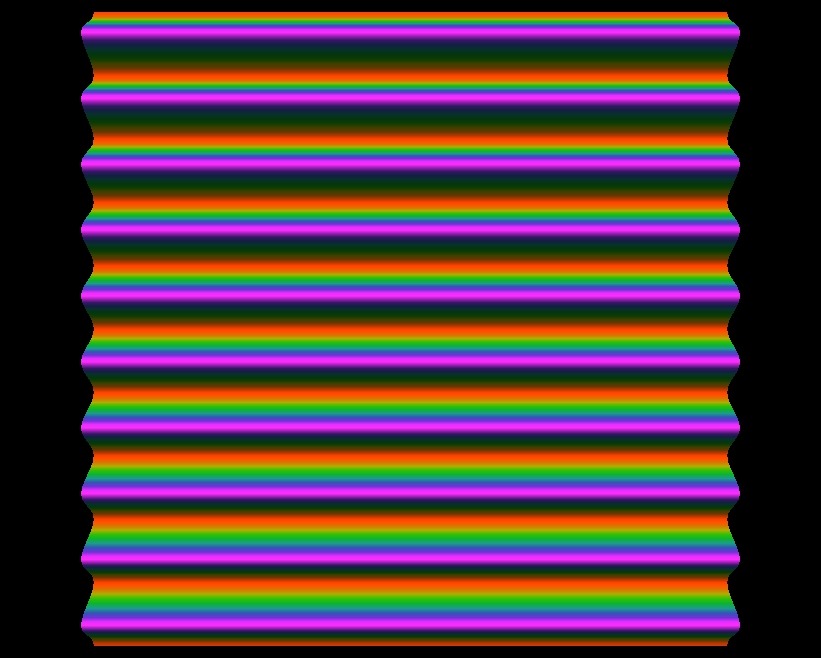
(a) $t=0$

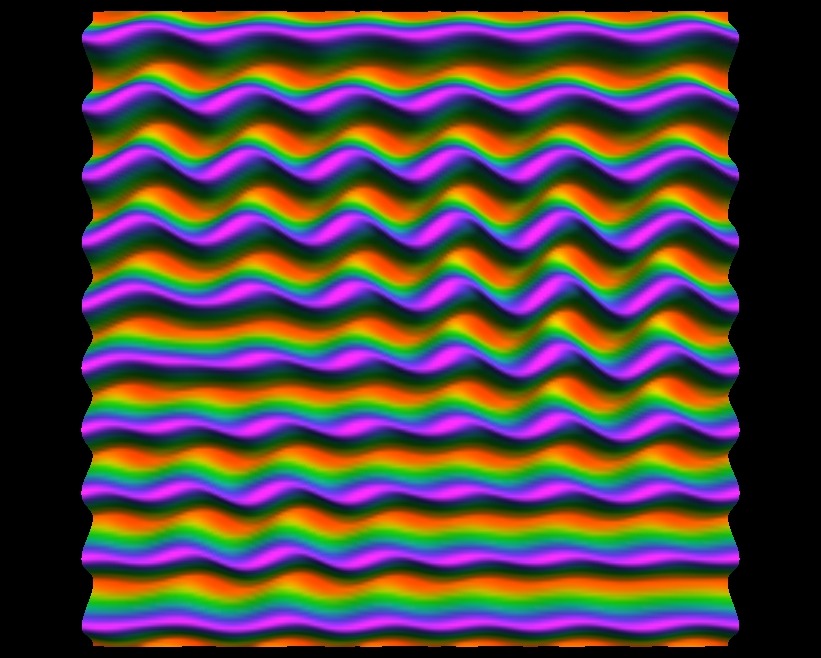
(b) $t=350$

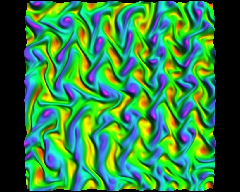
(c) $t=500$

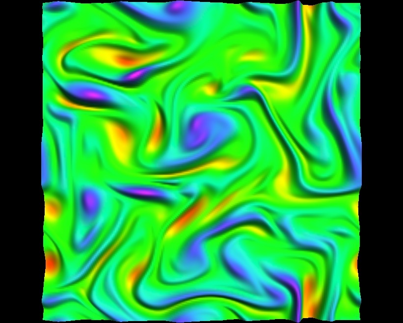
(d) $t=900$

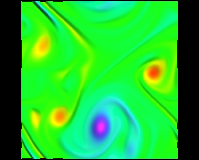
(e) $t=2500$

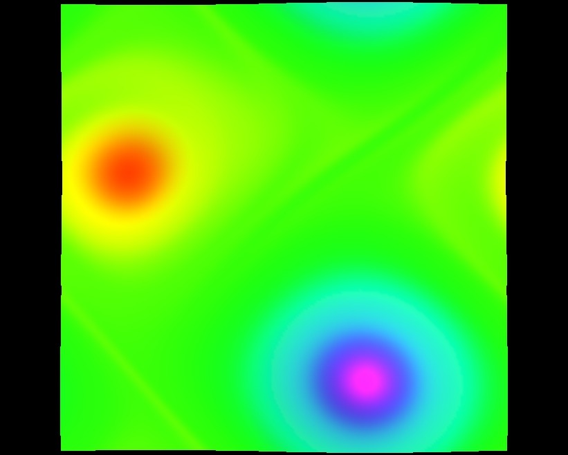
(f) $t=7000$

Figure 1: Vorticity field at various times for a turbulent run ($\rho_{0}=10^{10}$, $v_{0}=.05$, $D=10$, $n=10$). The inverse cascade behavior is evident, leading to two counter-rotating, and slowly decaying, vortices at late times.

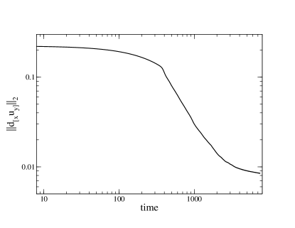
(a) Vorticity

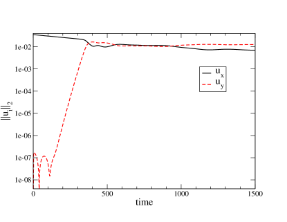
(b) Velocity

Figure 2: $L_{2}$ norms of (a) vorticity, and (b) $u_{i}$, as a function of time for turbulent flow (same run as Fig. 1). In (a) there is an initial exponential decay, followed by a power law during the inverse cascade, followed by a slower exponential decay. In (b) $u_{y}$ grows exponentially until it is of similar amplitude to $u_{x}$.

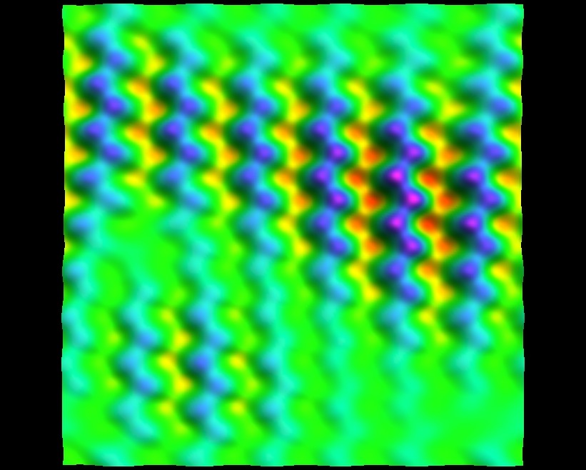
Figure 3: $u_{y}$ field at $t=300$ for the same run as Fig. 1.

At one extreme, the typical turbulent run is illustrated in Fig. 1. This shows the vorticity field at several times. In Fig. 2, we show the corresponding $L_{2}$ norms of the vorticity and the components of $u_{i}$. We see that initially, the vorticity and $u_{x}$ decay exponentially in the manner expected for shear flow. However, during that time, $\|u_{y}\|_{2}$ undergoes exponential growth, until it reaches the same amplitude as $\|u_{x}\|_{2}$. This brings the solution into an equipartition of energy between $u_{x}$ and $u_{y}$. At this point the initial decay has been disrupted, and turbulence sets in, as we will describe in more detail in the following subsections. The onset of this behavior is known as the Kelvin-Helmholtz instability in fluid dynamics.

Visual inspection of the $u_{y}$ field (see Fig. 3) indicates that the growing mode itself is also very roughly a shear mode,

$$u_{y}\approx f(t)\sin\left(\frac{2\pi my}{D}+\phi\right),$$ (41)

typically with $n/2<m<n$. As we have alluded to earlier, the finite box size plays a role at small $n$, and it comes into play here. For example, we find that the $n=1$ case is stable, even for large $R$, because the box does not admit a mode with $m<1$. This is the expected behavior as there is no room for an inverse cascade, given an $n=1$ initial configuration. For large $n$, there is no obstacle in fitting the growing mode into the box, and the box size $D$ plays no role. Thus, fixing $\lambda$ and extrapolating to the infinite box ($D\to\infty$), the instability should be present for sufficiently large $R$.

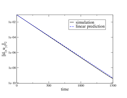
(a) Vorticity

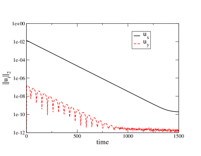
(b) Velocity

Figure 4: $L_{2}$ norms of (a) vorticity, and (b) $u_{i}$, as a function of time for a laminar flow. The norm of $u_{y}$ remains small throughout the decay. ($\rho_{0}=10^{7}$, $v_{0}=.02$, $D=10$, $n=10$)

At the other extreme, at low values of $R$, the flow is laminar. This is illustrated in Fig. 4. In contrast to the turbulent case, $\|u_{y}\|_{2}$ remains small throughout the run. ($u_{y}$ is being continuously driven nonlinearly by $u_{x}$, so its amplitude decays with $u_{x}$.) With small initial velocities, the linear analysis of Sec. III.1 is applicable, and the measured decay rate should be consistent with the prediction (34). Fig. 4a shows that this is indeed the case.

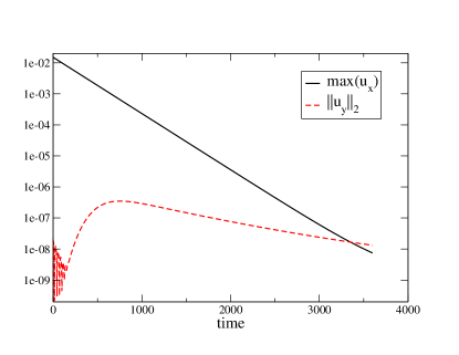
(a) Velocity

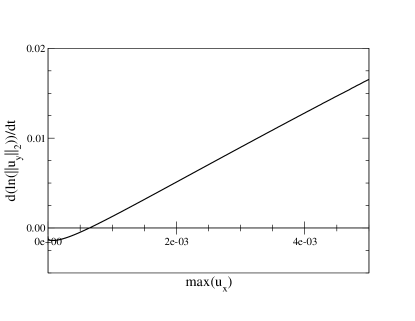
(b) Growth rate of $\|u_{y}\|_{2}$

Figure 5: Intermediate flow: (a) $u_{i}$, as a function of time for laminar flow, and (b) growth rate of $\|u_{y}\|_{2}$ versus $\max u_{x}$. The zero of (b) corresponds to the critical Reynolds number. ($\rho_{0}=10^{7}$, $v_{0}=.015$, $D=4$, $n=10$)

Between these two extremes, we found that there were certain intermediate flows which provided important physical information. Such an example is illustrated in Fig. 5. In this case, the flow begins at high Reynolds number but it decays before turbulence can fully develop. The plot of $\|u_{y}\|_{2}$ shows initially small perturbations growing nearly exponentially for some time – as in the turbulent case – before peaking, then decaying exponentially.

The time dependence of $R$ in such runs is clearly evident, as it is directly proportional to $\max(u_{x})$ (also plotted). Initially, $R>R_{c}$, but as time progresses, $R$ decreases. Since the background flow is slowly varying, we assume that the instantaneous growth rate of $\|u_{y}\|_{2}$ depends only on the background value of $\max(u_{x})$. Thus, at the peak of $\|u_{y}\|_{2}$, $R=R_{c}$, while for $R<R_{c}$, $\|u_{y}\|_{2}$ decays. This allows us to extract $R_{c}$. Indeed in Fig. 5b we plot the growth rate of $\|u_{y}\|_{2}$ versus $\max(u_{x})$. Where the curve crosses through zero corresponds to the peak of $\|u_{y}\|_{2}$ in Fig. 5a, and the value of $R_{c}$ may be read off. Thus, such intermediate runs provide detailed information on the stability of the background flow.

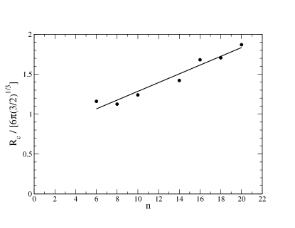
Figure 6: Critical Reynolds number as a function of wave number $n$ (dark circles). The solid line is the linear fit (42).

By searching for such critical runs (by adjusting $v_{0}$) for different values of $(\rho_{0},\,D,\,n)$, we found that the critical Reynolds number of the shear flow is

$$R_{c}\approx\left(\frac{3}{2}\right)^{1/3}6\pi\times 0.7\left(1+0.07n\right).$$ (42)

The dependence upon $n$ (see also Fig. 6) is due to the finite size of the box, as discussed above. We measured this within the range $6\leq n\leq 20$. (We verified, by varying also $\rho_{0}$ and $D$, that $R_{c}$ is independent of these quantities.) For large $n$, we expect $R_{c}$ to approach a limit, as the finite box size should play no role.

Fig. 5b also provides some information about the growth rate of $u_{y}$ away from its zero value at $R=R_{c}$. Fixing $n$ and $\rho_{0}$, this shows that for $R>R_{c}$, higher $R$ [higher $\max(u_{x})$] gives faster growth. For $R\gg R_{c}$, the growth rate is linear in $\max(u_{x})$. In contrast, as $R$ is lowered, there is a bound on the decay rate. This can be understood as a competition between a driving effect from the background shear flow in $u_{x}$, and a viscous decay (34) associated with the shear mode (41) in $u_{y}$. Once the driving term drops to the point of irrelevancy, all that is left is the decay term, which gives a fixed decay rate, as it is a property of the mode in $u_{y}$. Indeed, the asymptotic value of the growth rate of $\|u_{y}\|_{2}$ in Fig. 5b is -0.0013. This matches very nicely the prediction from Eq. (34) using the observed $m=6$.

We also found that for large $R$, the growth rate of $\|u_{y}\|_{2}$ is inversely proportional to $\lambda$, at fixed $\max(u_{x})$. Together with the above, this points to the contribution of the driving term to the growth rate as being proportional to $\partial_{y}u_{x}$.

IV.3 Turbulent regime

We now turn our attention back to the turbulent case, at the point where equipartition of energy is reached between $u_{y}$ and $u_{x}$ (i.e., just subsequent to Fig. 1b). As seen in Fig. 1c, the overall flow is completely disrupted, and the vorticity field displays a number of turbulent eddies. The exponential decay of vorticity in Fig. 2a ceases, and is replaced with a power law decay. We typically observed $\|\omega\|_{2}\propto t^{-\alpha}$, with $\alpha\simeq 1.2\pm 0.2$. There have been several previous studies of unforced turbulent decay of Navier-Stokes fluids in $d=3$, which have also found power law decays (e.g., Matthaeus et al. (1991); Smith et al. (1993); Huang and Leonard (1994)).

During the power law decay, the eddies merge into vortices, which continue to merge into increasingly large vortices (Figs. 1d and 1e). This inverse energy cascade can be attributed to the conservation of enstrophy Kraichnan (1967). Co-rotating vortices merge, while counter-rotating vorticies repel. Thus, one is finally left with two counter-rotating vortices, as in the inviscid case Carrasco et al. (2012).

IV.4 Late time decay

The vortices which form are the relativistic analog of the Oseen vortex, which is an attractor solution to the Navier-Stokes equation Gallay and Wayne (2005). Its functional form is

$$v_{\theta}=\frac{C_{1}}{r}\left(1-e^{-r^{2}/C_{2}(t)^{2}}\right),$$ (43)

where the parameter $C_{2}(t)=\sqrt{4\nu t}$, and the kinematic viscosity $\nu=\eta/\rho$. A fit for the parameters $C_{1}$ and $C_{2}$ is shown in Fig. 7.

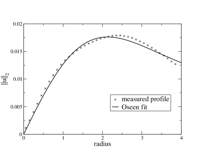
Figure 7: Velocity profile of one of the vortices in Fig. 1f. The solid line is the fit to the Oseen vortex profile.

We see that the vortex is close to, but does not match exactly, the Oseen profile. We attribute this to differences betwen Navier-Stokes fluids, and the relativistic compressible fluids we study. Fitting also in time, it is possible to extract $\nu$ from these profiles. As with the profile fit, we found a value of $\nu$ which, while not quite the predicted value, was within a factor of two.

At late times, the two vortices continue to decay in amplitude, until the fluid finally becomes linear. The solution is then the sum of long-wavelength shear and sound modes, which decay exponentially. We measured the decay rates at late times. The decay was slightly faster than the linear prediction, although the measured difference decreases at later times.

As a result of the increased wavelength, the decay rate at late times is lower than the decay rate of the initial flow. Thus, the presence of the turbulent cascade drastically lengthens the time period before the fluid settles down from its initial state to a uniform flow. In contrast, for $d>3$, where we expect a direct cascade, turbulence causes a more rapid decay than the linear behavior. This is due to higher modes decaying faster and strong dissipation at the viscous scale.

V Discussion: Black Branes and Turbulence

In the previous section, we have established conditions for the onset of turbulent phenomena in conformal, viscous relativistic fluids in $2+1$ dimensions, as well as the subsequent behavior once this develops. Having studied solutions to the dual hydrodynamic theory, we turn in this section to general relativity, and to the behavior of perturbed AAdS black holes and black branes.

V.1 Decay of perturbations and turbulence in the bulk

The decay properties of the shear fluid flow that we have analyzed in Sec. IV carry over directly to the shear hydrodynamic quasinormal mode of the black brane. Indeed, as described in the introduction, the gravity/fluid correspondence naturally captures the behavior of the lowest lying shear and sound families of quasinormal modes. (As illustrated in Ref. Adams et al. (2013), the higher order quasinormal modes typically decay very rapidly, and the metric produced via the duality is a very good approximation to a solution of Einstein’s equation.)

Translating to the black brane language, our results imply that, for $R>R_{c}$, hydrodynamic shear quasinormal modes are unstable to small perturbations (the “instability” refers to the quasinormal mode; not to the black brane). More precisely, certain deviations from the pure quasinormal mode undergo exponential growth until either they reach the amplitude of the quasinormal mode (fully developed turbulence) or the Reynolds number – which decays in time – becomes smaller than $R_{c}$ and an exponential decay ensues. Once turbulence sets in, for 4-dimensional AAdS black branes, energy is transferred to longer wavelength modes and a polynomial decay is induced. Eventually, when metric deviations about the uniform black brane become small enough, exponential decay resumes. In both cases, the final decay is at a slower rate than the original decay, as the perturbation is of longer wavelength.

On the other hand, for $R<R_{c}$, the quasinormal mode is stable, so it exhibits the usual clean exponential decay. We stress that in all cases described, the global norm of the solution decays in time.

More generally, one is interested in the behavior of a generic black brane perturbation, containing many modes of small but comparable magnitude. The standard picture states that if the amplitude of the perturbation is small enough, then at sufficiently late times it asymptotically approaches a sum of quasinormal modes, which evolve in time independently. However, the question is how small the amplitude must be for this to be realized; this is determined by the Reynolds number. At high Reynolds number, certain quasinormal modes are unstable; and an unstable mode will never be realized in a decay. The new picture that emerges is that of both laminar and turbulent phases. The laminar phase corresponds to the standard quasinormal mode picture. At high Reynolds number, however, the decaying perturbation immediately enters the turbulent phase, which has been uncovered through the gravity/fluid correspondence.

This new turbulent phase displays a far richer phenomenology. Our results indicate that turbulence, when it develops, induces eddies. Eddies with vorticity of the same sign merge, leading to increasingly large vortices as time proceeds Melander et al. (1988). The form of the bulk metric [to leading order, Eq. (2)], indicates that the boundary fluid structure is carried unperturbed along ingoing null geodesic “tubes” Bhattacharyya et al. (2008b), connecting the boundary at spatial infinity to the black brane event horizon. Thus the Oseen-like vortices present at late times in the turbulent fluid solution describe rather compact distributions of gravitational radiation connecting the asymptotic and black hole regions. They can be regarded as natural realizations of “extended geons”, which extend through the bulk as “gravitational tornadoes” or “funnels”. The structure that we describe is illustrated in Fig. 8, where we plot the curvature invariants $I_{1}$ and $I_{2}$ (see Appendix B).

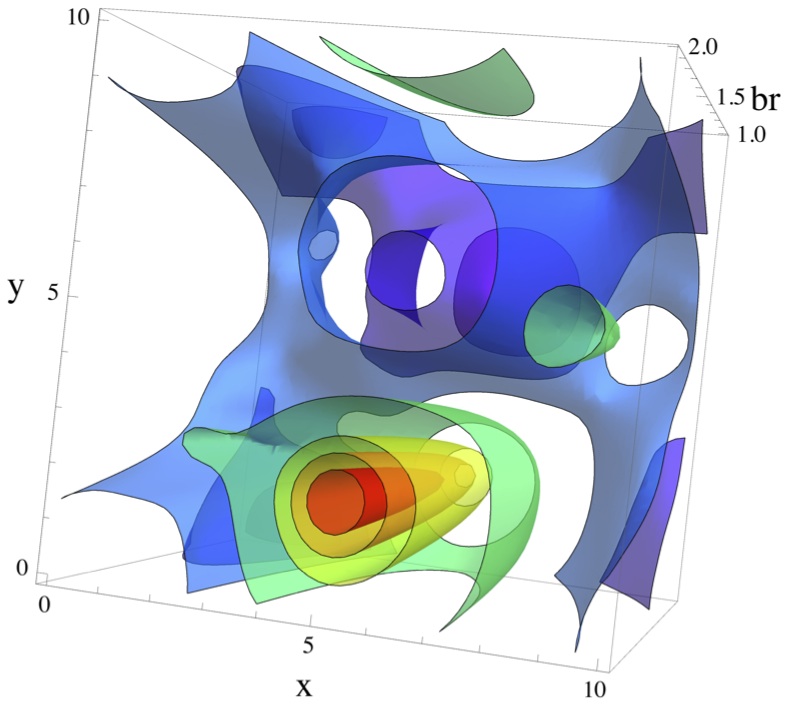
(a) $r^{6}\,C_{ABCD}C^{ABCD}$

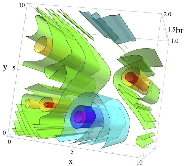
(b) $r^{7}\,{}^{*}C_{ABCD}C^{ABCD}$

Figure 8: Contour plots of principal invariants of the Weyl tensor in the bulk, computed from the zeroth order metric (2), from the simulation snapshot in Fig. 1e. Notice that (a) is representative of the energy density $\rho$, while (b) is representative of the vorticity, as expected from Eq. (89).

As discussed in Appendix A, a possible way to understand this behavior is related to the fact that a map to relativistic hydrodynamics is also possible away from the boundary, at suitably defined timelike surfaces in the bulk. Thus, the solution can also be analyzed at these surfaces to show, in particular, that a conserved quantity related to the enstrophy can be defined away from the boundary. Such a quantity is a key element needed to argue that an inverse energy cascade occurs.

Naturally, as already pointed out in Evslin (2012), it would be very useful to develop a spacetime definition of the Reynolds number. This would provide an intrinsic way to predict the onset of turbulence in gravity and could thus be applied in broader contexts. Using the gravity/fluid correspondence, this would also lead to a Reynolds number suitable for relativistic hydrodynamics. Based upon the form of the bulk metric (2), and the fluid Reynolds number (38), the form of the Reynolds number for black hole perturbations is, roughly,

$$R_{GR}\propto T_{\text{Hawking}}\left\|h_{AB}\left(\frac{\partial}{\partial r}\right)^{B}\right\|L,$$ (44)

where we have substituted (certain components of) the metric perturbation $h_{AB}\equiv g_{AB}-g_{AB}^{(0)}$ for the velocity fluctuation; and $L$ is the characteristic length scale of the perturbation. Of course, whether or not this is applicable in more general contexts would require further investigation. In particular, a suitable definition of $R$ should be gauge invariant.

As a final comment, we point out an important application of the fact that the inverse cascade guarantees the system stays within the domain of validity of the gravity/fluid correspondence. The relativistic hydrodynamic equations in $2+1$ dimensions are dual to (long-wavelength) perturbed black branes in the bulk. Thus, a Newtonian limit in the bulk – where time derivatives are taken to be one-order subleading to space derivatives and velocities are taken to also be small – corresponds to a Navier-Stokes limit on the boundary. Since we know that the Navier-Stokes equation admits global, well-behaved solutions Ladyzhenskaya (1969), one can surmise that general relativity is similarly well-behaved in the bulk.

V.2 Connection to ordinary perturbation theory

Linear perturbation theory predicts that small-amplitude metric perturbations can be decomposed (asymptotically) into independent modes which undergo simple exponential decay. On the other hand, the picture described in the previous section indicates the presence of a qualitatively distinct, turbulent, behavior for sufficiently high Reynolds numbers, regardless of the perturbation amplitude. How are these two notions reconciled? The short answer is that at very high black hole temperatures (in AdS), the regime of applicability of linear perturbation theory is very small. To study this further, we take a closer look at perturbation theory.

In ordinary perturbation theory, the full metric is expanded as

$$g_{AB}=g_{AB}^{(0)}+h_{AB}^{(1)}+h_{AB}^{(2)}+\ldots,$$ (45)

where $g_{AB}^{(0)}$ is taken to be the background metric; in our case, the uniform AdS black brane. The first order metric perturbation $h_{AB}^{(1)}$ satisfies the homogeneous partial differential equation,

$$G_{AB}^{(1)}(g^{(0)},h^{(1)})+\Lambda h_{AB}^{(1)}=0,$$ (46)

where $G_{AB}^{(1)}(g^{(0)},h^{(1)})$ is the linearized Einstein tensor. For the black brane, the symmetry properties admit a mode decomposition, and by solving Eq. (46), the quasinormal mode spectrum is determined. All of the modes decay for the AdS black brane Berti et al. (2009); Morgan et al. (2009).

At second order in perturbation theory,

$$G_{AB}^{(1)}(g^{(0)},h^{(2)})+\Lambda h_{AB}^{(2)}=-G^{(2)}_{AB}(g^{(0)},h^{(1)}),$$ (47)

where the second order Einstein tensor on the right hand side is quadratic in the first order perturbation $h^{(1)}_{AB}$. Since the homogeneous part of this equation is unchanged from the first order case, the quasinormal mode spectrum of $h_{AB}^{(2)}$ is also unchanged. These decaying modes are excited by the inhomogeneous source term. At any finite order in perturbation theory, the same applies. Thus, the growth we describe can be only captured by carrying out the analysis to sufficiently high orders in perturbation theory to recognize the underlying exponential behavior.

If, rather than taking the background metric $g_{AB}^{(0)}$ to be the uniform AdS black brane, it is instead taken to be the AdS black brane plus the shear hydrodynamic quasinormal mode, then the growth is easily seen to be possible at the linearized level (46). This is best illustrated through a simple toy model of ordinary differential equations (inspired by a local analysis of the Navier-Stokes equations) which exhibits similar mode-coupling properties, namely

$$\frac{dx}{dt}+\alpha x =0,$$ (48)

$$\frac{dy}{dt}+\beta y-\gamma xy =0,$$ (49)

with $\alpha$, $\beta$, and $\gamma$ all positive constants. The variable $x(t)$ in this system corresponds to $u_{y}$ in the black brane system, which initially describes a shear mode. On the other hand, $y(t)$ corresponds to the initially zero $u_{y}$. Both $x$ and $y$ are subject to dissipation (in the black brane case, $\alpha\approx\beta$), and we have included a mode-coupling $\gamma xy$ in (49).

Let us solve the system (48)–(49) perturbatively in two different ways. We expand both $x$ and $y$ as

$$x =x_{(0)}+x_{(1)}+x_{(2)}+\ldots,$$ (50)

$$y =y_{(0)}+y_{(1)}+y_{(2)}+\ldots.$$ (51)

The exact solution to (48) is $x\propto e^{-\alpha t}$. In a manner analogous to perturbation theory about the uniform black brane, we take the “background solution” to be $x_{(0)}=y_{(0)}=0$, while the “linearized solution” corresponds to the quasinormal mode, i.e., $x_{(1)}=a_{1}e^{-\alpha t}$. Then, the equation for $y_{(1)}$ is

$$\frac{dy_{(1)}}{dt}+\beta y_{(1)}=0,$$ (52)

with solution $y_{(1)}=b_{1}e^{-\beta t}$. At second order,

$$\frac{dy_{(2)}}{dt}+\beta y_{(2)}=\gamma x_{(1)}y_{(1)}=\gamma a_{1}b_{1}e^{-(\alpha+\beta)t}.$$ (53)

The solution to this is $y_{(2)}=-a_{1}b_{1}\gamma e^{-(\alpha+\beta)t}/\alpha+b_{2}e^{-\beta t}$; higher order corrections can be computed in a similar manner. At each order in perturbation theory the solution is a sum of decaying exponentials.

Suppose instead that we take $x_{(0)}=a_{0}e^{-\alpha t}$ and $y_{(0)}=0$. This is analogous to taking the black brane perturbed by a quasinormal mode as the “background solution”. Then, at linear order we have

$$\frac{dy_{(1)}}{dt}+\beta y_{(1)}=\gamma x_{(0)}y_{(1)}=\gamma a_{0}e^{-\alpha t}y_{(1)},$$ (54)

which has solution $y_{(1)}=b_{1}\exp\left[-\beta t+a_{0}\gamma\left(1-e^{-\alpha t}\right)/\alpha\right]$. In the limit of small $\alpha$, this becomes

$$y_{(1)}\xrightarrow{\alpha\to 0}b_{1}e^{-(\beta-a_{0}\gamma)t}.$$ (55)

Thus, if the “background” is long-lived, the growth rate of $y$ depends upon a competition between the driving term $\gamma xy$ and the dissipative term $\beta y$. For finite $\alpha>0$, the driving term decreases with time relative to the dissipative term. In this case, $y_{(1)}$ is eventually dominated by the exponential decay (cf. Fig. 5).

One can define a “Reynolds number” of the flow $x(t)$ in the toy model, by taking the ratio of the mode-coupling term $\gamma xy$, to the linear dissipative term, $\beta y$, in (49). If this “Reynolds number”, $\gamma a_{0}e^{-\alpha t}/\beta$, is large, then the nonlinear term $\gamma xy$ should be kept in any perturbative analysis, and one should solve Eq. (54) – rather than Eq. (52) – to determine $y$.

A similar story holds in for black brane perturbations in general relativity. The problem with trying to analyze high Reynolds number perturbations by performing ordinary perturbation theory about the uniform black brane background, is that this drops certain large nonlinear terms while keeping small linear terms. For the black brane, the dissipation rate (the analog of $\alpha\approx\beta$) depends inversely on the temperature. So, increasing the temperature, while holding fixed the amplitude and wavelength of a perturbation (i.e., increasing the Reynolds number), the linear term evantually becomes small relative to nonlinear terms. Thus, the regime of validity of ordinary perturbation theory is reduced as the Reynolds number is increased.

V.3 Beyond 4-d AAdS black branes

Here we discuss some possible implications and extensions of this work.

V.3.1 Higher dimensions

Based upon our results for 4-dimensional bulk spacetimes, together with the gravity/fluid correspondence established in arbitrary dimensions, as well as numerical results confirming the expectation of direct energy cascades for inviscid conformal relativistic fluids Radice and Rezzolla (2013), it is possible to anticipate properties of 5 (and higher) dimensional spacetimes (for an early discussion, see Van Raamsdonk (2008)). Three immediate consequences are:

• First, as with the 4-dimensional case, at sufficiently high Reynolds number, the quasinormal mode description fails to accurately describe the decay of black brane perturbations.

• Second, in contrast to the 4-dimensional case, turbulence is characterized by a direct energy cascade to short wavelengths. Since shorter wavelengths have a more rapid decay rate, thermalization in 5 dimensions will be attained in a shorter timescale than in an analog 4-dimensional case. Notice that a potential concern here is that the cascade to short wavelengths may cause the solution to exit the regime of validity of the gravity/fluid correspondence. Two comments are relevant here. (i) Even if this were the case, perturbations initially satisfying $LT\gg 1$ (as required by the correspondence) still undergo turbulent dynamics which induce structure at shorter wavelengths. Thus, at the moment of “exiting” the regime of validity, many modes would be present and their subsequent behavior should be studied within general relativity. (ii) It is also possible for the cascade to occur completely within the regime of validity of the correspondence if the viscous scale (again defined as in the non-relativistic case) $L_{\eta}=(\eta^{3}/\epsilon)^{1/4}$ (where $\epsilon$ is the rate of energy dissipation by viscosity) satisfies $L_{\eta}T\gg 1$. Notice that $L_{\eta}$ grows with temperature, so at sufficiently high $T$, this condition is satisfied. In this case energy would be expected to cascade down to the viscous scale, and then dissipate.

  As a consequence of the turbulent behavior on the hydrodynamical side – which displays a self-similar behavior – one would expect a similar (fractal) structure for black hole perturbations on the gravitational side. This structure is expected to smooth out in time yielding a slightly hotter, uniform black brane. If this is the case, then in this high temperature limit [case (ii)], a global solution to the dual relativistic hydrodynamics problem would seem to be a natural consequence. As in the $d=2+1$ fluid case, this would have obvious implications for global solutions to the Navier-Stokes equation. Establishing this decay result rigorously on the gravity side amounts to determining nonlinear stability of large black holes in AdS.

• Finally, a word of caution with regard to nonlinear numerical studies of gravitational perturbations in 5 dimensions: Due to the high computational cost of such simulations, symmetries are usually imposed on the solution, effectively reducing the number of dimensions which are actually simulated. However, this may restrict or affect the development of turbulence. In particular, 5-dimensional spacetimes which are dimensionally reduced to 4 dimensions will give rise to an inverse energy cascade – rather than a direct one – while 3-dimensional treatments will eliminate turbulence altogether. As one is often interested in using the AdS/CFT correspondence to describe high temperature CFTs through a gravitational analysis, it is important to bear in mind that the imposition of computation-saving symmetries can impact the extracted physics.

V.3.2 Black holes

We have investigated the decay of black branes in a Poincaré patch of AdS, with torus topology. However, it is also of interest to study black holes in global AdS. Based on earlier work in the inviscid case Carrasco et al. (2012), we expect a qualitatively similar turbulent behavior. One primary difference, though, is the final number of vortices which remain (e.g., fluids dual to Kerr-Schwarzschild settle down to two clockwise and two counter-clockwise rotating vortices, while Kerr-AdS settles to just one of each sign). Other particular details, such as the power law decay rate during turbulence, and the critical Reynolds number, may also differ. The power law behavior, $\|\omega\|_{2}\propto t^{-\alpha}$, can also be estimated in the inviscid case. An examination of results presented in Carrasco et al. (2012) indicates that for black holes, the decaying behavior is realized with a similar exponent to black branes, in the range $0.5<\alpha<1.5$.

V.3.3 Beyond AdS

At a speculative but certainly tantalizing level, that gravity displays turbulent behavior in AAdS spacetimes suggests that more general asymptotic conditions should also be investigated. Is this a special property of AdS, or could it arise in the asymptotically flat or de Sitter cases? What about Dirichlet boundary conditions, but without a cosmological constant? There are two elements to consider: The boundary conditions imposed on the solutions to the Einstein equation, and the presence of the cosmological constant in the equation of motion. From a partial differential equations point of view the cosmological constant introduces a lower order term in the equations, which does not affect local propagation.

On the other hand, it is well known that linearized perturbations of AAdS black hole spacetimes have a family of very slowly decaying modes (the hydrodynamic modes), which (as we have shown) play a key role in terms of being unstable to perturbations. Such modes are also present in certain vacuum solutions bounded by an accelerating mirror, which have been shown to be dual to Navier-Stokes fluids Bredberg et al. (2012). Interestingly, at least some hydrodynamic modes can also be connected to QNMs of asymptotically flat spacetimes Dias et al. (2013). However, in this regime, the modes decay rapidly, and therefore do not govern the long term behavior of the system. However, they could play a role in channeling energy in the transient stages. Furthermore, it is well known that massive fields introduce effective boundaries which could induce the long-lived mode behavior, and thus allow for turbulent-like phenomena. As discussed earlier, if a Reynolds number can be suitably defined for gravity, it would help predict the onset of turbulence in these varied scenarios.

V.4 Final words

As we have stressed throughout this work, the gravity/fluid correspondence translates intuition of fluid behavior into the realm of gravity. This has allowed us to identify key features of the behavior of perturbed AAdS black holes, including a new dynamical phase where fully developed “turbulence” gives rise to a polynomial decay. Furthermore, turbulent behavior also indicates that perturbed black holes can behave in a strongly dimensionally-dependent way, both qualitatively and quantitatively. Establishing that gravity can behave in a turbulent manner opens new doors to searching for other situations where this can take place. For instance, it provides motivation to look for scenarios where slowly decaying perturbations might give rise to interesting non-linear interactions. Finally, insights from turbulence may shed new light on particular systems known to exhibit related behavior, such as the chaotic behavior of spacelike singularities in early-universe mixmaster dynamics Evslin (2012).

Appendix A Spacetime Turbulence: Bulk Behavior and Radial Map to Relativistic Hydrodynamics

As mentioned, the gravity/fluid correspondence indicates that the boundary behavior is manifested throughout the bulk. Consequently, one expects an inverse cascade behavior which mirrors the behavior at the boundary. Here we provide further details on how this behavior can be seen to arise. In particular, we show how a conserved current (in the high temperature limit that approaches the inviscid case) gives rise to a conserved enstrophy.

A.1 Preliminary considerations: Boundary quantities and enstrophy

To first order, and now with an arbitrary boundary metric $\gamma_{\mu\nu}$, the bulk metric can be written in the form Bhattacharyya et al. (2008b)

$$ds^{2}_{[0+1]}=-2u_{\mu}dx^{\mu}(dr+r{\cal A}_{\nu}dx^{\nu})+r^{2}\left(\gamma_{\mu\nu}+\frac{1}{(br)^{d}}u_{\mu}u_{\nu}+2bF(br)\sigma_{\mu\nu}\right)dx^{\mu}dx^{\nu}.$$ (56)

Here, $\mathcal{A}_{\nu}\equiv a_{\nu}-\frac{1}{2}\Theta u_{\nu}$, where $\Theta\equiv\nabla_{\mu}u^{\mu}$ is the expansion of the velocity field $u^{\mu}$, and $a^{\mu}$ its acceleration.

At the AdS boundary, the following quantities can be defined:

• The stress-energy tensor Balasubramanian and Kraus (1999); Henningson and Skenderis (1998),

  $$T^{\mu}_{\phantom{\mu}\nu}\equiv\lim_{r\to\infty}\frac{r^{d}}{8\pi G_{d+1}}(K_{\phantom{\mu}\nu}^{\mu}-\delta^{\mu}_{\nu}K),$$ (57)

  where $K_{\phantom{\mu}\nu}^{\mu}$ is the extrinsic curvature of a constant-$r$ hypersurface. To first order in the derivative expansion, this is

  $$T_{\mu\nu}^{[0+1]}=(\rho+P)u_{\mu}u_{\nu}+P\gamma_{\mu\nu}-2\eta\sigma_{\mu\nu}.$$ (58)

• Conserved currents. In the high temperature limit, the effects of viscosity are subleading. Thus, if $\gamma_{\mu\nu}$ admits a timelike Killing vector field $\xi^{\mu}$, then in this limit, conservation of stress-energy gives rise to conservation of the energy current Carrasco et al. (2012),

  $$J^{\mu}_{\rho}\equiv\frac{1}{2}\rho(\gamma^{\mu\nu}+3u^{\mu}u^{\nu})\xi_{\nu}.$$ (59)

  Again in the inviscid limit, there is also a conserved enstrophy current Carrasco et al. (2012),

  $$J^{\mu}_{Z}\equiv\omega^{\alpha\beta}\omega_{\alpha\beta}u^{\mu}.$$ (60)

A.2 Bulk behavior: Radial map and enstrophy

The steps above can be extended into the bulk by considering $r=\text{constant}$ timelike hypersurfaces. Within the regime of validity of the gradient expansion, such hypersurfaces are timelike outside the black brane horizon.

It is possible to project the Einstein equation onto a constant-$r$ hypersurface, in order to obtain a fluid description on the hypersurface Brattan et al. (2011); Kuperstein and Mukhopadhyay (2011). As in the $r\to\infty$ limit addressed earlier, the “momentum constraint” gives rise to a conserved stress-energy tensor $\hat{T}_{\mu\nu}$. It turns out to be of the same form as the boundary stress-energy, with

$$\hat{T}_{\mu\nu}=(\hat{\rho}+\hat{P})\hat{u}_{\mu}\hat{u}_{\nu}+\hat{P}\hat{\gamma}_{\mu\nu}-2\eta\hat{\sigma}_{\mu\nu}+\ldots.$$ (61)

These new (hatted) fields $\hat{\gamma}_{\mu\nu}$, $\hat{p}$, $\hat{u}_{\mu}$, $\hat{\rho}$ and $\hat{\sigma}_{\mu\nu}$ are related to the original fields at the boundary through a map, which, to first order in derivatives, gives Brattan et al. (2011); Kuperstein and Mukhopadhyay (2011)

$$\hat{\gamma}_{\mu\nu} =\gamma_{\mu\nu}+\left(1-\frac{1}{\alpha^{2}}\right)u_{\mu}u_{\nu}+2bF(br)\sigma_{\mu\nu}-\frac{2}{r}u_{(\mu}\mathcal{A}_{\nu)}+\ldots,$$ (62)

$$\hat{\gamma}^{\mu\nu} =\gamma^{\mu\nu}+\left(1-\alpha^{2}-\frac{\alpha^{4}\Theta}{r}\right)u^{\mu}u^{\nu}-2bF(br)\sigma^{\mu\nu}+\frac{2\alpha^{2}}{r}u^{(\mu}a^{\nu)}+\ldots,$$ (63)

$$\hat{u}_{\mu} =\left(1-\frac{\alpha^{2}\Theta}{2r}\right)\frac{u_{\mu}}{\alpha}+\frac{\alpha}{r}a_{\mu},$$ (64)

$$\hat{u}^{\mu} =\left(1+\frac{\alpha^{2}\Theta}{2r}\right)\alpha u^{\mu}+\ldots,$$ (65)

$$\hat{\rho} =\frac{2\alpha}{\alpha+1}\rho,$$ (66)

$$\hat{P} =\frac{\alpha}{\alpha+1}(3\alpha-1)P,$$ (67)

$$\hat{\omega}_{\mu\nu} =\frac{1}{\alpha}\omega_{\mu\nu},$$ (68)

where $\alpha\equiv\left(1-\frac{1}{(br)^{3}}\right)^{-1/2}=\left(1-\frac{8\pi G_{4}}{r^{3}}\rho\right)^{-1/2}$.

A crucial difference with respect to the boundary fluid is that now the fluid “lives” on a background $\hat{\gamma}_{\mu\nu}$, which is dynamical. In addition, this fluid obeys a more complicated equation of state,

$$\hat{P}=\frac{(3\alpha(\hat{\rho})-1)}{4}\hat{\rho},$$ (69)

where $\alpha(\hat{\rho})=\left(1-\frac{4\pi G_{4}}{r^{3}}\hat{\rho}\right)^{-1}$. Connected with this last point, the stress-tensor is no longer traceless,

$$\hat{T}_{\phantom{\mu}\mu}^{\mu}=\frac{3\alpha(\alpha-1)}{(\alpha+1)}\rho=-r\frac{d\hat{\rho}}{dr}.$$ (70)

This has been interpreted as an RG flow Brattan et al. (2011); Kuperstein and Mukhopadhyay (2011, 2013), in which the radius $r$ plays the role of an energy scale from the field theory perspective.

Keeping in mind these differences, it is still the case that each constant-$r$ timelike hypersurface contains a relativistic fluid description, just like the AdS boundary. Thus, similar conservation laws can be derived. Of particular interest is the existence of an enstrophy which, in the high temperature limit, is conserved. To define this quantity for a general equation of state $\hat{P}(\hat{\rho})$, only a slight generalization of the previous derivation is required.

We begin with the inviscid fluid equations,

$$u^{\nu}\partial_{\nu}\rho =-(\rho+P)\nabla_{\mu}u^{\mu},$$ (71)

$$P^{\mu\nu}\partial_{\nu}P =-(\rho+P)u^{\nu}\nabla_{\nu}u^{\mu}.$$ (72)

Next, we will require a function $\tilde{\rho}(\rho)$ such that the 2-form $\Omega_{\mu\nu}\equiv 2\nabla_{[\mu}(\tilde{\rho}u_{\nu]})$ satisfies $\Omega_{\mu\nu}u^{\nu}=0$. This is accomplished by choosing

$$\tilde{\rho}(\rho)\propto(\rho+P)\exp\left[-\int\frac{d\rho^{\prime}}{\rho^{\prime}+P(\rho^{\prime})}\right],$$ (73)

where the exponent contains an indefinite integral, and we assumed the integration can be performed for a given equation of state $P(\rho)$.

Notice that $\Omega_{\mu\nu}$, is strongly conserved by the flow by virtue of Cartan’s identity. That is,

$$\textbf{\pounds}_{\lambda\mathbf{u}}\mathbf{\Omega}=\lambda\mathbf{u}\cdot\mathbf{d\Omega}+\mathbf{d}(\lambda\mathbf{u}\cdot\mathbf{\Omega})=0.$$ (74)

Motivated by this observation, we can construct a current of the form $J_{Z}^{\mu}\equiv\lambda\Omega^{2}u^{\mu}$, where we have denoted $\Omega_{\alpha\beta}\Omega^{\alpha\beta}\equiv\Omega^{2}$, and $\lambda$ a scalar field to be fixed by the conservation requirement. Computing the divergence of $J^{\mu}$ one obtains,

$$\nabla_{\mu}J_{Z}^{\mu} =\Omega^{2}\left[\lambda\nabla_{\mu}u^{\mu}+u^{\mu}\partial_{\mu}\lambda\right]+2\lambda\Omega^{\sigma\beta}u^{\mu}\partial_{\mu}\Omega_{\sigma\beta}$$

$$=\Omega^{2}\left[\lambda\nabla_{\mu}u^{\mu}+u^{\mu}\partial_{\mu}\lambda\right]-4\lambda\Omega^{\sigma\beta}\Omega_{\sigma\mu}(\nabla_{\beta}u^{\mu})$$

$$=\Omega^{2}\left[u^{\mu}\partial_{\mu}\lambda-\lambda\nabla_{\mu}u^{\mu}\right].$$ (75)

We have used the definition of the Lie derivative and (74) on the second line, and the third line follows from,

$$\Omega^{\mu\alpha}\Omega_{\mu\beta}=\frac{1}{2}\Omega^{2}P^{\alpha}_{\phantom{\alpha}\beta},$$ (76)

an identity which is valid in two spatial dimensions Carrasco et al. (2012). Clearly, the divergence in Eq. (A.2) vanishes if $\lambda(\rho)\propto\exp\left[-\int\frac{d\rho^{\prime}}{\rho^{\prime}+P(\rho^{\prime})}\right]$.

Notice also that $\Omega^{2}$ is related to the square vorticity ($\omega^{2}\equiv\omega_{\mu\nu}\omega^{\mu\nu}$) by $\Omega^{2}=4\tilde{\rho}^{2}\omega^{2}$. Finally, by integrating the current $J_{Z}^{\mu}$ over a constant-$t$ hypersurface $\Sigma_{t}$, the expression for the enstrophy takes the form

$$Z\equiv\int_{\Sigma_{t}}\gamma(\rho+P)^{2}\exp\left[-3\int\frac{d\rho^{\prime}}{\rho^{\prime}+P(\rho^{\prime})}\right]\omega^{2}dS^{2}.$$ (77)

It is straightforward to check that this expression reduces to the one reported previously in Carrasco et al. (2012) for the conformal fluid on the boundary,

$$Z_{\text{boundary}}=\int_{\Sigma_{t}}\gamma\omega^{2}dS^{2}\,,$$ (78)

when the equation of state is given by $P(\rho)=\frac{1}{2}\rho$.

We are now in a position to evaluate the enstrophy on an arbitrary $r=\text{constant}$ timelike hypersurface in terms of boundary variables,

$$Z(r)=\int_{\Sigma_{t}(r)}\hat{\omega}^{2}(\hat{\rho}+\hat{P})^{2}\exp\left[-3\int\frac{d\hat{\rho}^{\prime}}{\hat{\rho}^{\prime}+\hat{P}(\hat{\rho}^{\prime})}\right]\hat{u}^{\mu}d\hat{\Sigma}_{\mu}.$$ (79)

From Eqs. (69) and (66) we get,

$$(\hat{\rho}+\hat{P})^{2}\exp\left[-3\int\frac{d\hat{\rho}^{\prime}}{\hat{\rho}^{\prime}+\hat{P}(\hat{\rho}^{\prime})}\right]=\left(\frac{3}{8}\right)^{2}\alpha^{2},$$ (80)

while for the square vorticity we find that,

$$\hat{\omega}^{2}=\frac{1}{\alpha^{2}}\omega^{2}.$$ (81)

As a final remark, let us note that to zeroth order in the gradient expansion, the transformation from one surface element to the other is given by

$$\hat{u}^{\mu}d\hat{\Sigma}_{\mu}=u^{\mu}d\Sigma_{\mu}.$$ (82)

Consequently, the enstrophy calculated at any given radius $r$, not only is conserved, but is also equivalent (up to an unimportant constant factor which can be trivially absorbed into the definition) to the enstrophy of the boundary fluid. That is,

$$Z(r)\sim Z_{\text{boundary}}.$$ (83)

The fact that it is possible to define an enstrophy for the fluid on each slice of the bulk geometry, and that it has the same expression in all cases, is a natural consequence of the ultra-local character of the map. Thus, in a sense, the dynamics occurring at the boundary are reproduced throughout the bulk geometry (in a slightly distorted manner). At first sight, this enstrophy construction in the bulk seems to indicate that one could define an interesting local quantity from the spacetime perspective in the bulk. However, since this quantity is defined on a distorted (and dynamical) surface, one should exercise caution, especially in highly distorted scenarios.

Appendix B Bulk Behavior: Geometrical Quantities

It is also instructive to examine the bulk through geometrical quantities. This is particularly appealing as it could provide a geometrical way to understand fluid phenomena. Such a program, however, is delicate, since an unambiguous definition of local quantities is not generally possible in general relativity. One possible way to do so is to construct gauge invariant quantities, together with a judicious choice of coordinates to specify the points at which these quantities are evaluated. Two useful scalars can be constructed via the Riemann tensor. These are the Kretschmann $K_{1}\equiv R_{ABCD}R^{ABCD}$ and the Chern-Pontryagin $K_{2}\equiv{}^{*}R_{ABCD}R^{ABCD}$ scalars. Related to these, the principal invariants of the Weyl tensor are $I_{1}\equiv C_{ABCD}C^{ABCD}$ and $I_{2}\equiv{}^{*}C_{ABCD}C^{ABCD}$. In addition, Newman-Penrose scalars are useful to describe particular characteristics of the solution.

Here, we evaluate these quantities in the case of a single vortex on the boundary. Since the vortices we have seen are approximately axially symmetric, it is convenient to introduce boundary coordinates $(t,\varrho,\phi)$. The boundary functions then take the form $\rho=\rho(\varrho),u_{\varrho}=0,u_{\phi}=u_{\phi}(\varrho)$, where we set $\varrho=0$ at the center of the vortex. With this assumption, the zeroth order bulk metric (2) takes the form,

$$ds^{2}_{[0]}=-2u_{\mu}dx^{\mu}dr+\left(r^{2}P_{\mu\nu}-F(r,\varrho)u_{\mu}u_{\nu}\right)dx^{\mu}dx^{\nu}.$$ (84)

Here, $F(r,\varrho)=\frac{\rho(\varrho)}{r}$, and the horizon is located at $r=\rho(\varrho)$ to zeroth order.

We also introduce the following null tetrad:

$$l^{A} =\partial_{r}^{A},$$ (85)

$$n^{A} =u_{0}\partial_{t}^{A}-\frac{1}{2}(r^{2}-F(r,\varrho))\partial_{r}^{A}-\frac{u_{\phi}}{\varrho^{2}}\partial_{\phi}^{A},$$ (86)

$$m^{A} =\frac{u_{\phi}}{\sqrt{2}r\varrho}\partial_{t}^{A}+i\frac{1}{\sqrt{2}r}\partial_{\varrho}^{A}-\frac{u_{0}}{\sqrt{2}r\varrho}\partial_{\phi}^{A},$$ (87)

which satisfies $-l^{A}n_{A}=m^{A}\bar{m}_{A}=1$. With the tetrad, we construct the Newman-Penrose scalars, $\Psi_{0}=C_{ABCD}l^{A}m^{B}l^{C}m^{D}$, $\Psi_{1}=C_{ABCD}l^{A}n^{B}l^{C}m^{D}$, $\Psi_{2}=C_{ABCD}l^{A}m^{B}\bar{m}^{C}n^{D}$, $\Psi_{3}=C_{ABCD}l^{A}n^{B}\bar{m}^{C}n^{D}$, $\Psi_{4}=C_{ABCD}n^{A}\bar{m}^{B}n^{C}\bar{m}^{C}$, which are related to the mass aspect, angular momentum and radiation in the system.

We evaluate all of these quantities for our vortex solution to leading order, and in the non-relativistic case,

$$K_{1} \sim 12\left(2+\frac{\rho(\varrho)^{2}}{r^{6}}\right)\,\,,\,\,K_{2}\sim 36\frac{\rho(\varrho)^{2}}{r^{7}}\omega\,,$$ (88)

$$I_{1} \sim 12\frac{\rho(\varrho)^{2}}{r^{6}}\,\,,\,\,I_{2}\sim 36\frac{\rho(\varrho)^{2}}{r^{7}}\omega\,,$$ (89)

$$\Psi_{0}=0\,\,,\,\,\Psi_{1}\sim\frac{\sqrt{2}}{8\varrho r^{3}}\omega\,\,,\,\,\Psi_{2} \sim -\frac{\rho(\varrho)}{2r^{3}}-i\frac{3\rho(\varrho)}{4r^{4}}\omega\,\,,\,\,\Psi_{3}\sim-\frac{\sqrt{2}(r^{3}+\rho(\varrho))}{8\varrho r^{4}}\omega\,\,,\,\,\Psi_{4}\sim-i\frac{3\rho(\varrho)}{4r^{2}\varrho^{2}}(\varrho^{2}\omega-2u_{\phi})\,.$$ (90)

(evaluation of the horizon is obtained by $r\rightarrow\rho(\varrho)^{1/3}$). Notice that $\Psi_{4}$ is purely imaginary, which implies a single polarization of gravitational waves due to the axisymmetric structure of the vortex.

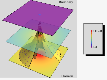
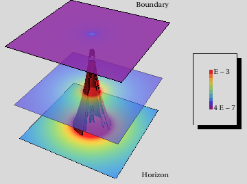
Figure 9: Contour plots for $\Psi_{1}$, $\Im(\Psi_{2})$ and $\Psi_{3}$ (left to right) illustrating the vortex structure from the horizon to the boundary. Note that the “conical” structure is a result of the dependence upon the radial coordinate of the plotted quantities (see Eq. (89)). (In contrast to Fig. 8, we are not rescaling here by any powers of $r$.)

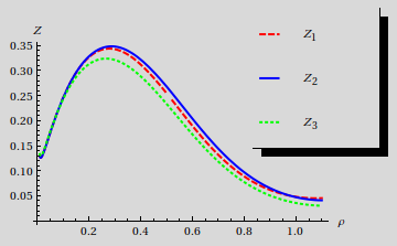
Figure 10: Radial profile of the “enstrophy” at the horizon, for a vortex solution, as calculated by Eq. (79), the square of the Pontryagin density Adams et al. (2013), and $[\Im(\Psi_{2})]^{2}$ Eling and Oz (2013) (labelled $Z_{1},Z_{2}$ and $Z_{3}$, respectively). Each curve has been rescaled by a trivial constant factor for easier comparison.

Notice that most of these curvature quantities depend to leading order on the vorticity. In fact, they are related through the identity $I_{1}-i\,I_{2}=16(3\,\Psi_{2}^{2}+\Psi_{0}\Psi_{4}-4\Psi_{1}\Psi_{3})$. Thus, there is some freedom in choosing which curvature quantities to use to analyze the structure which arises in the bulk. Fig. 9 displays the behavior of $\Psi_{1},\Im(\Psi_{2})$ and $\Psi_{3}$ as functions of $(r,\varrho,\phi)$ at fixed $t$, while Fig. 8 illustrates the behavior of $I_{1}$ and $I_{2}$ for one of the solutions we obtained in our simulations. Recent works have proposed several different curvature quantities to represent the enstrophy. For instance, at the horizon, the squares of $K_{2}$ and $\Im(\Psi_{2})$, respectively, have been suggested in Adams et al. (2013) and Eling and Oz (2013). These quantities can be extended throughout the bulk and compared with the quantity introduced in Appendix A.2. Fig. 10 illustrates the radial profile of the three quantities, showing good agreement.

References

- Maldacena (1998) J. M. Maldacena, Adv. Theor. Math. Phys. 2, 231 (1998), arXiv:hep-th/9711200 [hep-th] .
- Aharony et al. (2000) O. Aharony, S. S. Gubser, J. M. Maldacena, H. Ooguri, and Y. Oz, Phys. Rept. 323, 183 (2000), arXiv:hep-th/9905111 [hep-th] .
- Baier et al. (2008) R. Baier, P. Romatschke, D. T. Son, A. O. Starinets, and M. A. Stephanov, JHEP 0804, 100 (2008), arXiv:0712.2451 [hep-th] .
- Bhattacharyya et al. (2008a) S. Bhattacharyya, V. E. Hubeny, S. Minwalla, and M. Rangamani, JHEP 0802, 045 (2008a), arXiv:0712.2456 [hep-th] .
- Bhattacharyya et al. (2008b) S. Bhattacharyya, R. Loganayagam, I. Mandal, S. Minwalla, and A. Sharma, JHEP 0812, 116 (2008b), arXiv:0809.4272 [hep-th] .
- Van Raamsdonk (2008) M. Van Raamsdonk, JHEP 0805, 106 (2008), arXiv:0802.3224 [hep-th] .
- Oz and Rabinovich (2011) Y. Oz and M. Rabinovich, JHEP 1102, 070 (2011), arXiv:1011.5895 [hep-th] .
- Eling et al. (2010) C. Eling, I. Fouxon, and Y. Oz, (2010), arXiv:1004.2632 [hep-th] .
- Carrasco et al. (2012) F. Carrasco, L. Lehner, R. C. Myers, O. Reula, and A. Singh, Phys. Rev. D86, 126006 (2012), arXiv:1210.6702 [hep-th] .
- Radice and Rezzolla (2013) D. Radice and L. Rezzolla, Astrophys. J. 766, L10 (2013), arXiv:1209.2936 [astro-ph.HE] .
- Kraichnan (1967) R. H. Kraichnan, Physics of Fluids 10, 1417 (1967).
- Adams et al. (2013) A. Adams, P. M. Chesler, and H. Liu, (2013), arXiv:1307.7267 [hep-th] .
- Berti et al. (2009) E. Berti, V. Cardoso, and A. O. Starinets, Class. Quant. Grav. 26, 163001 (2009), arXiv:0905.2975 [gr-qc] .
- Morgan et al. (2009) J. Morgan, V. Cardoso, A. S. Miranda, C. Molina, and V. T. Zanchin, JHEP 0909, 117 (2009), arXiv:0907.5011 [hep-th] .
- Kovtun and Starinets (2005) P. K. Kovtun and A. O. Starinets, Phys. Rev. D72, 086009 (2005), arXiv:hep-th/0506184 [hep-th] .
- Israel (1976) W. Israel, Annals Phys. 100, 310 (1976).
- Israel and Stewart (1976) W. Israel and J. Stewart, Physics Letters A 58, 213 (1976).
- Israel and Stewart (1979) W. Israel and J. Stewart, Annals Phys. 118, 341 (1979).
- Evslin (2012) J. Evslin, Fortsch. Phys. 60, 1005 (2012), arXiv:1201.6442 [hep-th] .
- Wald (1984) R. M. Wald, General Relativity (University of Chicago Press, Chicago, IL, 1984).
- Haack and Yarom (2008) M. Haack and A. Yarom, JHEP 0810, 063 (2008), arXiv:0806.4602 [hep-th] .
- Balasubramanian and Kraus (1999) V. Balasubramanian and P. Kraus, Commun. Math. Phys. 208, 413 (1999), arXiv:hep-th/9902121 [hep-th] .
- Eckart (1940) C. Eckart, Phys. Rev. 58, 919 (1940).
- Hiscock and Lindblom (1983) W. A. Hiscock and L. Lindblom, Annals of Physics 151, 466 (1983).
- Geroch (1995) R. P. Geroch, J. Math. Phys. 36, 4226 (1995).
- Geroch (2001) R. P. Geroch, (2001), arXiv:gr-qc/0103112 [gr-qc] .
- LeVeque (2002) R. J. LeVeque, Finite-Volume Methods for Hyperbolic Problems (Cambridge University Press, 2002).
- Luzum and Romatschke (2008) M. Luzum and P. Romatschke, Phys. Rev. C78, 034915 (2008), arXiv:0804.4015 [nucl-th] .
- Romatschke (2010) P. Romatschke, Int. J. Mod. Phys. E19, 1 (2010), arXiv:0902.3663 [hep-ph] .
- Calabrese et al. (2003) G. Calabrese, L. Lehner, D. Neilsen, J. Pullin, O. Reula, et al., Class. Quant. Grav. 20, L245 (2003), arXiv:gr-qc/0302072 [gr-qc] .
- Calabrese et al. (2004) G. Calabrese, L. Lehner, O. Reula, O. Sarbach, and M. Tiglio, Class. Quant. Grav. 21, 5735 (2004), arXiv:gr-qc/0308007 [gr-qc] .
- Landau and Lifshitz (1987) L. D. Landau and E. M. Lifshitz, Fluid Mechanics (Butterworth-Heinemann, Oxford, UK, 1987).
- Matthaeus et al. (1991) W. H. Matthaeus, W. T. Stribling, D. Martinez, S. Oughton, and D. Montgomery, Phys. Rev. Lett. 66, 2731 (1991).
- Smith et al. (1993) M. R. Smith, R. J. Donnelly, N. Goldenfeld, and W. F. Vinen, Phys. Rev. Lett. 71, 2583 (1993).
- Huang and Leonard (1994) M.-J. Huang and A. Leonard, Physics of Fluids 6, 3765 (1994).
- Gallay and Wayne (2005) T. Gallay and C. E. Wayne, Commun. Math. Phys. 255, 97 (2005), arXiv:math/0402449 .
- Evslin and Krishnan (2010) J. Evslin and C. Krishnan, JHEP 1010, 028 (2010), arXiv:1007.4452 [hep-th] .
- Warnick (2013) C. M. Warnick, (2013), arXiv:1306.5760 [gr-qc] .
- Melander et al. (1988) M. Melander, N. Zabusky, and J. McWilliams, Journal of Fluid Mechanics 195, 303 (1988).
- Hubeny et al. (2010) V. E. Hubeny, D. Marolf, and M. Rangamani, Class. Quant. Grav. 27, 025001 (2010), arXiv:0909.0005 [hep-th] .
- Bhattacharyya et al. (2009) S. Bhattacharyya, S. Minwalla, and S. R. Wadia, JHEP 0908, 059 (2009), arXiv:0810.1545 [hep-th] .
- Bredberg et al. (2012) I. Bredberg, C. Keeler, V. Lysov, and A. Strominger, JHEP 1207, 146 (2012), arXiv:1101.2451 [hep-th] .
- Ladyzhenskaya (1969) O. A. Ladyzhenskaya, The mathematical theory of viscous incompressible flow, Second English edition, revised and enlarged. Translated from the Russian by Richard A. Silverman and John Chu. Mathematics and its Applications, Vol. 2 (Gordon and Breach Science Publishers, New York, 1969).
- Lehner and Pretorius (2010) L. Lehner and F. Pretorius, Phys. Rev. Lett. 105, 101102 (2010), arXiv:1006.5960 [hep-th] .
- Holzegel and Smulevici (2013) G. Holzegel and J. Smulevici, (2013), arXiv:1303.5944 [gr-qc] .
- Holzegel and Smulevici (2011) G. Holzegel and J. Smulevici, (2011), arXiv:1110.6794 [gr-qc] .
- Dias et al. (2013) O. J. Dias, G. S. Hartnett, J. E. Santos, V. Cardoso, and L. Lehner, in preparation (2013).
- Henningson and Skenderis (1998) M. Henningson and K. Skenderis, JHEP 9807, 023 (1998), arXiv:hep-th/9806087 [hep-th] .
- Eling and Oz (2013) C. Eling and Y. Oz, (2013), arXiv:1308.1651 [hep-th] .
- Brattan et al. (2011) D. Brattan, J. Camps, R. Loganayagam, and M. Rangamani, JHEP 1112, 090 (2011), arXiv:1106.2577 [hep-th] .
- Kuperstein and Mukhopadhyay (2011) S. Kuperstein and A. Mukhopadhyay, JHEP 1111, 130 (2011), arXiv:1105.4530 [hep-th] .
- Kuperstein and Mukhopadhyay (2013) S. Kuperstein and A. Mukhopadhyay, (2013), arXiv:1307.1367 [hep-th] .