Stationary Cycling Induced by Switched Functional Electrical Stimulation Control

Abstract

Functional electrical stimulation (FES) is used to activate the dysfunctional lower limb muscles of individuals with neuromuscular disorders to produce cycling as a means of exercise and rehabilitation. In this paper, a stimulation pattern for quadriceps femoris-only FES-cycling is derived based on the effectiveness of knee joint torque in producing forward pedaling. In addition, a switched sliding-mode controller is designed for the uncertain, nonlinear cycle-rider system with autonomous state-dependent switching. The switched controller yields ultimately bounded tracking of a desired trajectory in the presence of an unknown, time-varying, bounded disturbance, provided a reverse dwell-time condition is satisfied by appropriate choice of the control gains and a sufficient desired cadence. Stability is derived through Lyapunov methods for switched systems, and experimental results demonstrate the performance of the switched control system under typical cycling conditions.

I Introduction

Since the 1980s, cycling induced by functional electrical stimulation (FES) has been investigated as a safe means of exercise and rehabilitation for people with lower-limb paresis or paralysis [1], and numerous physiological and psychological benefits have since been reported [2]. Despite these benefits, FES-cycling is still metabolically inefficient and results in low power output compared to volitional cycling by able-bodied individuals [3], [4]. Many approaches have been taken in attempt to improve the efficiency and power output of FES-cycling, including optimization of the cycling mechanism [5], [6], alteration of the stimulation pattern [7, 8, 9, 10, 11], and variation of the stimulation strategy [12, 13, 14, 15]. Studies have explored the use of feedback control methods to automatically determine the appropriate stimulation parameters, but most use either linear approximations of the nonlinear cycle-rider system [16] or nonlinear methods lacking detailed stability analyses [17, 18, 19]. Previous approaches (cf. [20], [21]) often either determine the stimulation pattern manually by stimulating a particular muscle group and observing the resulting crank motion or base the stimulation pattern on electromyography recordings of able-bodied cyclists. Stimulation frequency is then fixed and stimulation intensity is typically controlled by varying the magnitude of a predefined trapezoidal stimulation signal proportional to the cycling cadence error. All of the aforementioned studies used stimulation patterns which switch between active muscle groups according to the crank position, resulting in a switched control system with autonomous state-dependent switching [22]. However, no study has yet investigated FES-cycling control in the context of switched systems theory. Switched systems may be unstable even if each subsystem is asymptotically stable [22], so the switching logic must be taken into account in the control design to guarantee stability of the system. In general, switched control of FES-cycling involves switching between stabilizable and unstable, uncertain, nonlinear dynamics, yet no previous studies have addressed this aspect of FES-cycling. Therefore, studying FES-cycling in this light could potentially reveal new control methods.

In this paper, a nonlinear model of the cycle-rider system is considered with parametric uncertainty and an unknown, time-varying, bounded disturbance, and the stability of the closed-loop switched control system is analyzed via Lyapunov methods. A stimulation pattern for the quadriceps femoris muscle groups of the rider is derived based on the kinematic effectiveness of knee joint torque at producing forward pedaling throughout the crank cycle. The stimulation pattern is designed so that stimulation is not applied in regions near the dead points of the cycle to bound the stimulation voltage, while everywhere else in the crank cycle either the right or left quadriceps are stimulated to produce forward pedaling. Since the quadriceps are stimulated without overlap, the crank cycle is composed of controlled and uncontrolled regions. Stimulation of additional muscle groups, e.g., the gluteal muscles, could eliminate the uncontrolled regions but it could also result in overlapping controlled regions and over-actuation; thus, only stimulation of the quadriceps is considered in this paper. In the controlled regions, a switched sliding-mode controller for the stimulation intensity is designed which guarantees exponentially stable tracking of the desired crank trajectory provided sufficient gain conditions are satisfied. In the uncontrolled regions, the tracking error is proven to be bounded provided a reverse dwell-time condition is satisfied, which requires that the system must not dwell in the uncontrolled region for an overly long time interval [23]. The reverse dwell-time condition is shown to be satisfied provided sufficient desired cadence conditions are satisfied. The tracking error is then proven to converge to an ultimate bound as the number of crank cycles approaches infinity. Experimental results are provided which demonstrate the performance of the switched controller for typical cycling conditions.

II Model

II-A Stationary Cycle and Rider Dynamic Model

The subsequent development is based on a stationary cycle and a two-legged rider that are modeled as a single degree-of-freedom system [24], which can be expressed as

$$M\ddot{q}+V\dot{q}+G+\tau_{d}-\tau_{b}-P=\sum_{s\in\mathcal{S}}B_{k}^{s}\Omega^{s}u^{s},$$ (1)

where $q\in\mathcal{Q}\subseteq\mathbb{R}$ denotes the crank angle, defined as the clockwise angle between the ground and the right crank arm, $M\in\mathbb{R}$ denotes inertial effects, $V\in\mathbb{R}$ represents centripetal and Coriolis effects, $G\in\mathbb{R}$ represents gravitational effects, $\tau_{d}\in\mathbb{R}$ represents an unknown, time-varying, bounded disturbance (e.g., changes in load), $\tau_{b}\triangleq-c\dot{q}$ represents viscous damping in the crank joint bearings where $c\in\mathbb{R}_{>0}$ is the unknown constant damping coefficient, $P\in\mathbb{R}$ captures the passive viscoelastic effects of the rider’s joints on the crank’s motion, $B_{k}\in\mathbb{R}$ is the Jacobian element relating torque about the knee to torque about the crank, and $\Omega\in\mathbb{R}$ is an uncertain nonlinear function relating the quadriceps stimulation voltage $u\in\mathbb{R}$ to the active torque at the knee. The superscript $s\in\mathcal{S}\triangleq\left\{R,\>L\right\}$ denotes right ($R$) and left ($L$) sides of the model (i.e., right and left legs and crank arms) and is omitted unless it adds clarity. The rider’s legs are modeled as planar rigid-body segments with revolute hip and knee joints (more complex models of the knee joint have a negligible effect on the linkage kinematics [25]). The ankle joint is assumed to be fixed in accordance with common clinical cycling practices for safety and stability [7]. When the rider’s feet are fixed to the pedals, the resulting system’s position and orientation can be completely described by the crank angle (or any other single joint angle measured with respect to ground), the kinematic parameters of the limb segments, and the horizontal and vertical components of the distance between the axes of rotation of the crank and hip joints, $l_{x},\>l_{y}\in\mathbb{R}_{\geq 0},$ respectively. The model in (1) has the following properties[26, 27, 28].

Property 1.

$c_{m}\leq M\leq c_{M},$ where $c_{m},\>c_{M}\in\mathbb{R}_{>0}$ are known constants. Property 2. $\left|V\right|\leq c_{V}\left|\dot{q}\right|$, where $c_{V}\in\mathbb{R}_{>0}$ is a known constant. Property 3. $\left|G\right|\leq c_{G},$ where $c_{G}\in\mathbb{R}_{>0}$ is a known constant. Property 4. $\left|\tau_{d}\right|\leq c_{d},$ where $c_{d}\in\mathbb{R}_{>0}$ is a known constant. Property 5. $\left|B_{k}^{s}\right|\leq c_{B}$ $\forall s\in\mathcal{S},$ where $c_{B}\in\mathbb{R}_{>0}$ is a known constant. Property 6. $\left|P\right|\leq c_{P1}+c_{P2}\left|\dot{q}\right|$, where $c_{P1},\>c_{P2}\in\mathbb{R}_{>0}$ are known constants. Property 7. $c_{\Omega 1}\leq\Omega^{s}\leq c_{\Omega 2}\>\forall s\in\mathcal{S},$ where $c_{\Omega 1},\>c_{\Omega 2}\in\mathbb{R}_{>0}$ are known constants. Property 8. $\frac{1}{2}\dot{M}-V=0.$

II-B Switched System Model

The torque transfer ratios $B_{k}^{s}$ give insight into how the quadriceps muscles of each leg should be activated during the crank cycle. By convention, the quadriceps can only produce a counter-clockwise torque about the knee joint that acts to extend the knee. Multiplication of the active knee torque by $B_{k}$ transforms the counter-clockwise torque produced by the quadriceps to a resultant torque about the crank. Therefore, since forward pedaling requires a clockwise torque about the crank, the quadriceps muscles should only be activated when they produce a clockwise torque about the crank, i.e., when $B_{k}$ is negative. The torque transfer ratio $B_{k}$ is negative definite for half of the crank cycle and the sign of the torque transfer ratio of one leg is always opposite that of the other leg (i.e., $B_{k}^{R}B_{k}^{L}\leq 0\>\forall q$), provided the crank arms are offset by $\pi$ radians. To induce pedaling using only FES of the quadriceps muscles, a controller must stimulate muscles on each leg in an alternating pattern, using the right quadriceps when $B_{k}^{R}<0$, the left quadriceps when $B_{k}^{L}<0$, and switching between muscle groups when $B_{k}=0.$ The torque transfer ratios $B_{k}^{s}$ are zero only at the so-called dead points $q^{*}\in\mathcal{Q}^{*}\subset\mathcal{Q}$, where $\mathcal{Q}^{*}\triangleq\left\{q\in\mathcal{Q}\>|\>q=\mbox{arctan}\left(l_{y}/l_{x}\right)+i\pi\right\},\>i\in\mathbb{Z}.$

Since the torque transfer ratios are minimal near the dead points, stimulation applied close to the dead points is inefficient in the sense that large knee torques yield small crank torques. Therefore, in the subsequent development, the uncontrolled region in which no stimulation is applied is defined as $\mathcal{Q}_{u}\triangleq\left\{q\in\mathcal{Q}\>|\>-B_{k}\left(q\right)\leq\varepsilon\right\}\subset\mathcal{Q},$ where $\varepsilon\in\mathbb{R}_{>0}$ is a scalable constant that can be increased to reduce the portion of the cycle trajectory where stimulation is applied. Specifically, $\varepsilon<\mbox{max}\left(-B_{k}\right).$ Also let the sets $\mathcal{Q}^{s}\subset\mathcal{Q}$ be defined as the regions where the right and left quadriceps muscle groups are stimulated, as

$$\mathcal{Q}^{s}\triangleq\left\{q\in\mathcal{Q}\>|\>-B_{k}^{s}\left(q\right)>\varepsilon\right\},$$ (2)

and denote the set $\mathcal{Q}_{c}\triangleq\cup_{s\in\mathcal{S}}\mathcal{Q}^{s}$ as the controlled region, where $\mathcal{Q}_{c}\cup\mathcal{Q}_{u}=\mathcal{Q}$ and $\mathcal{Q}^{R}\cap\mathcal{Q}^{L}=\textrm{\O},$ i.e., stimulation voltage is never applied to both legs at the same time. The stimulation pattern is then completely defined by the cycle-rider kinematics (i.e., $B_{k}$) and selection of $\varepsilon.$ Smaller values of $\varepsilon$ yield larger stimulation regions and vice versa. Some evidence in the FES-cycling literature (e.g., [8]) suggests that the stimulation region should be made as small as possible while maximizing stimulation intensity to optimize metabolic efficiency, motivating the selection of large values of $\varepsilon.$

Cycling is achieved by switching between stimulation of the left and right quadriceps muscle groups in an alternating pattern, where stimulation of the quadriceps occurs outside of $\mathcal{Q}_{u}$ to avoid the dead points and their neighborhoods where pedaling is inefficient. Specifically, the switched control input $u^{s}$ is designed as

$$u^{s}\triangleq\begin{cases}v&\mbox{if}\>q\in\mathcal{Q}_{c}\\ 0&\mbox{if}\>q\in\mathcal{Q}_{u}\end{cases},$$ (3)

where $v\in\mathbb{R}$ is the stimulation control input. Substitution of (3) into (1) yields a switched system with autonomous state-dependent switching as

$$M\ddot{q}+V\dot{q}+G+\tau_{d}-\tau_{b}-P=\begin{cases}B_{k}\Omega v&\mbox{if}\>q\in\mathcal{Q}_{c}\\ 0&\mbox{if}\>q\in\mathcal{Q}_{u}\end{cases}.$$ (4)

Assuming that $q$ starts inside $\mathcal{Q}_{c}$, the known sequence of switching states is defined as $\left\{q_{n}^{on},\>q_{n}^{off}\right\},$ $n\in\left\{0,\>1,\>2,\>...\right\}$, where $q_{0}^{on}$ is the initial crank angle and the switching states which follow are the limit points of $\mathcal{Q}_{u}.$ The subsequent analysis is facilitated by defining the corresponding sequence of switching times $\left\{t_{n}^{on},\>t_{n}^{off}\right\},$ which are unknown a priori, where each on-time $t_{n}^{on}$ and off-time $t_{n}^{off}$ occurs when $q$ reaches the corresponding on-angle $q_{n}^{on}$ and off-angle $q_{n}^{off},$ respectively. Fig. 1 illustrates controlled and uncontrolled regions, along with the switching states and dead points, throughout the crank cycle.

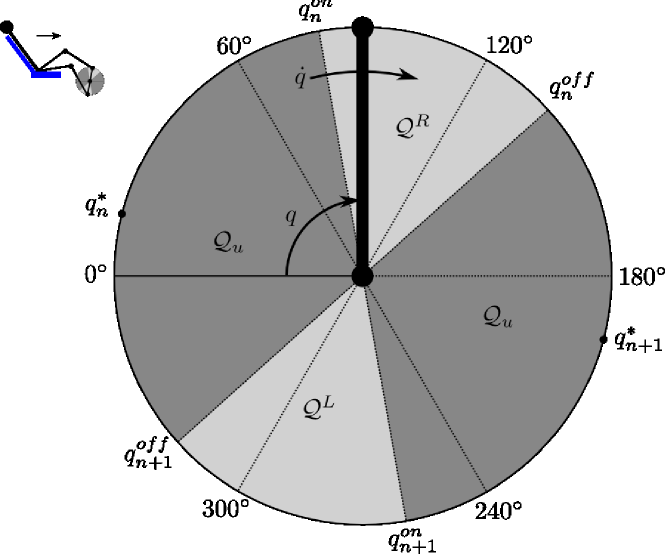
Figure 1: Controlled and uncontrolled regions throughout the crank cycle, along with the switching states and dead points. Lightly shaded regions are the controlled regions, and darkly shaded regions are the uncontrolled regions.

III Control Development

III-A Open-Loop Error System

The control objective is to track a desired crank trajectory with performance quantified by the tracking error signals $e_{1},\>e_{2}\in\mathbb{R}$, defined as

$$e_{1} \triangleq q_{d}-q,$$ (5)

$$e_{2} \triangleq \dot{e}_{1}+\alpha e_{1},$$ (6)

where $q_{d}\in\mathbb{R}$ is the desired crank position, designed so that its derivatives exist, and $\dot{q}_{d},\>\ddot{q}_{d}\in\mathcal{L}_{\infty},$ and $\alpha\in\mathbb{R}_{>0}$ is a selectable constant. Without loss of generality, $q_{d}$ is designed to monotonically increase, i.e., stopping or backpedaling is not desired. Taking the time derivative of (6), multiplying by $M,$ and using (4)-(6) yields the following open-loop error system:

$$M\dot{e}_{2}=\chi-Ve_{2}-\begin{cases}B_{k}\Omega v&\mbox{if}\>q\in\mathcal{Q}_{c}\\ 0&\mbox{if}\>q\in\mathcal{Q}_{u}\end{cases},$$ (7)

where the auxiliary term $\chi\in\mathbb{R}$ is defined as

$$\chi\triangleq M\left(\ddot{q}_{d}+\alpha\dot{e}_{1}\right)+V\left(\dot{q}_{d}+\alpha e_{1}\right)+G+\tau_{d}-\tau_{b}-P.$$ (8)

Based on (8) and Properties 1-6, $\chi$ can be bounded as

$$\left|\chi\right|\leq c_{1}+c_{2}\left\|z\right\|+c_{3}\left\|z\right\|^{2},$$ (9)

where $c_{1},\>c_{2},\>c_{3}\in\mathbb{R}_{>0}$ are known constants and the error vector $z\in\mathbb{R}^{2}$ is defined as

$$z\triangleq\left[\begin{array}[]{cc}e_{1}&e_{2}\end{array}\right]^{T}.$$ (10)

III-B Closed-Loop Error System

Based on (7) and the subsequent stability analysis, the control voltage input is designed as

$$v\triangleq-k_{1}e_{2}-\left(k_{2}+k_{3}\left\|z\right\|+k_{4}\left\|z\right\|^{2}\right)\mbox{sgn}\left(e_{2}\right),$$ (11)

where $\mbox{sgn}\left(\cdot\right)$ denotes the signum function and $k_{1},\>k_{2},\>k_{3},\>k_{4}\in\mathbb{R}_{>0}$ are constant control gains. After substituting (11) into the open-loop error system in (7), the following switched closed-loop error system for $q\in\mathcal{Q}_{c}$ is obtained:

$$M\dot{e}_{2} = \chi-Ve_{2}+B_{k}\Omega\biggl{[}k_{1}e_{2}$$ (12)

$$+\biggl{(}k_{2}+k_{3}\left\|z\right\|+k_{4}\left\|z\right\|^{2}\biggr{)}\mbox{sgn}\left(e_{2}\right)\biggr{]}.$$

The controller in (11) could also include $\left(B_{k}\right)^{-1}$ to cancel the preceding $B_{k}$ since it is known, resulting in less conservative gain conditions. However, doing so would cause sharp increases of the control input near the uncontrolled regions, depending on the choice of $\varepsilon$, resulting in undesirably large magnitude stimulation of the muscles in regions where their effectiveness is low.

IV Stability Analysis

Let $V_{L}\>:\>\mathbb{R}^{2}\rightarrow\mathbb{R}$ denote a continuously differentiable, positive definite, radially unbounded, common Lyapunov-like function defined as

$$V_{L}\triangleq\frac{1}{2}z^{T}Wz,$$ (13)

where the positive definite matrix $W\in\mathbb{R}^{2\times 2}$ is defined as

$$W\triangleq\left[\begin{array}[]{cc}1&0\\ 0&M\end{array}\right].$$ (14)

The function $V_{L}$ can be upper and lower bounded as

$$\lambda_{1}\left\|z\right\|^{2}\leq V_{L}\leq\lambda_{2}\left\|z\right\|^{2},$$ (15)

where $\lambda_{1},\>\lambda_{2}\in\mathbb{R}_{>0}$ are known constants defined as

$$\lambda_{1}\triangleq\mbox{min}\left(\frac{1}{2},\>\frac{c_{m}}{2}\right),\>\>\>\lambda_{2}\triangleq\mbox{max}\left(\frac{1}{2},\>\frac{c_{M}}{2}\right).$$

Theorem 1.

For $q\in\mathcal{Q}_{c}$, the closed-loop error system in (12) is exponentially stable in the sense that

$$\left\|z\left(t\right)\right\| \leq \sqrt{\frac{\lambda_{2}}{\lambda_{1}}}\left\|z\left(t_{n}^{on}\right)\right\|e^{-\frac{\gamma_{1}}{2\lambda_{2}}\left(t-t_{n}^{on}\right)}$$ (16)

$\forall t\in\left(t_{n}^{on},\>t_{n}^{off}\right)$ and $\forall n$, where $\gamma_{1}\in\mathbb{R}_{>0}$ is defined as

$$\gamma_{1}\triangleq\mathit{\mbox{min}}\left(\alpha-\frac{1}{2},\>\varepsilon c_{\Omega 1}k_{1}-\frac{1}{2}\right),$$ (17)

provided the following gain conditions are satisfied:

$$\alpha>\frac{1}{2},\>k_{1}>\frac{1}{2\varepsilon c_{\Omega 1}},\>k_{2}\geq\frac{c_{1}}{\varepsilon c_{\Omega 1}},$$

$$k_{3}\geq\frac{c_{2}}{\varepsilon c_{\Omega 1}},\>k_{4}\geq\frac{c_{3}}{\varepsilon c_{\Omega 1}}.$$ (18)

Proof:

Let $z\left(t\right)$ for $t\in\left(t_{n}^{on},\>t_{n}^{off}\right)$ be a Filippov solution to the differential inclusion $\dot{z}\in K\left[h\right]\left(z\right),$ where $K\left[\cdot\right]$ is defined as in [29] and where $h\>:\>\mathbb{R}\times\mathbb{R}\rightarrow\mathbb{R}^{2}$ is defined using (6) and (12) as

$$h\triangleq\left[\begin{array}[]{c}e_{2}-\alpha e_{1}\\ M^{-1}\biggl{\{}\chi-Ve_{2}+B_{k}\Omega\biggl{[}k_{1}e_{2}\\ \>\>\>+\left(k_{2}+k_{3}\left\|z\right\|+k_{4}\left\|z\right\|^{2}\right)\mbox{sgn}\left(e_{2}\right)\biggr{]}\biggr{\}}\end{array}\right].$$ (19)

The time derivative of (13) exists almost everywhere (a.e.), i.e., for almost all $t\in\left(t_{n}^{on},\>t_{n}^{off}\right),$ and $\dot{V}_{L}\left(z\right)\overset{a.e.}{\in}\dot{\tilde{V}}_{L}\left(z\right),$ where $\dot{\tilde{V}}_{L}$ is the generalized time derivative of (13) along the Filippov trajectories of $\dot{z}=h\left(z\right)$ and is defined as [30]

$$\dot{\tilde{V}}_{L}\triangleq\underset{\xi\in\partial V_{L}\left(z\right)}{\cap}\xi^{T}K\left[\begin{array}[]{c}h\left(z\right)\\ 1\end{array}\right],$$

where $\partial V_{L}$ is the generalized gradient of $V_{L}$. Since $V_{L}$ is continuously differentiable in $z$, $\partial V_{L}=\left\{\nabla V_{L}\right\};$ thus,

$$\dot{\tilde{V}}_{L}\subseteq\left[\begin{array}[]{c}z^{T}W\\ \frac{1}{2}z^{T}\dot{W}z\end{array}\right]^{T}K\left[\begin{array}[]{c}h\left(z\right)\\ 1\end{array}\right].$$

Using the calculus of $K$ from [30], substituting (19), and using (14) to simplify the resulting expression yields

$$\dot{\tilde{V}}_{L} \subseteq -\alpha e_{1}^{2}+e_{1}e_{2}+\chi e_{2}+\left(\frac{1}{2}\dot{M}-V\right)e_{2}^{2}$$ (20)

$$+B_{k}\Omega\left(k_{1}e_{2}^{2}\right)+B_{k}\Omega\biggl{(}k_{2}+k_{3}\left\|z\right\|$$

$$+k_{4}\left\|z\right\|^{2}\biggr{)}K\left[\mbox{sgn}\right]\left(e_{2}\right)e_{2},$$

where $K\left[\mbox{sgn}\right]\left(e_{2}\right)=1$ $\mbox{if}\>e_{2}>0,\>\left[-1,\>1\right]\>\mbox{if}\>e_{2}=0,$ and $-1\>\mbox{if}\>e_{2}<0.$ Using Property 8 and the fact that $\dot{V}_{L}\left(z\right)\overset{a.e.}{\in}\dot{\tilde{V}}_{L}\left(z\right)$ allows (20) to be rewritten as

$$\dot{V}_{L} \overset{a.e.}{=} -\alpha e_{1}^{2}+e_{1}e_{2}+\chi e_{2}+B_{k}\Omega\left(k_{1}e_{2}^{2}\right)$$ (21)

$$+B_{k}\Omega\left(k_{2}+k_{3}\left\|z\right\|+k_{4}\left\|z\right\|^{2}\right)\left|e_{2}\right|.$$

Note that $K\left[\mbox{sgn}\right]\left(e_{2}\right)$ is only set-valued for $e_{2}=0,$ so that $K\left[\mbox{sgn}\right]\left(e_{2}\right)e_{2}$ may be rewritten simply as $\left|e_{2}\right|,$ as was done in (21). By using Young’s inequality, (9), Property 7, and the fact that $B_{k}<-\varepsilon$ for $q\in\mathcal{Q}_{c}$, (21) can be upper bounded as

$$\dot{V}_{L} \overset{a.e.}{\leq} -\left(\alpha-\frac{1}{2}\right)e_{1}^{2}-\left(\varepsilon c_{\Omega 1}k_{1}-\frac{1}{2}\right)e_{2}^{2}$$ (22)

$$+\left(c_{1}-\varepsilon c_{\Omega 1}k_{2}\right)\left|e_{2}\right|+\left(c_{2}-\varepsilon c_{\Omega 1}k_{3}\right)\left\|z\right\|\left|e_{2}\right|$$

$$+\left(c_{3}-\varepsilon c_{\Omega 1}k_{4}\right)\left\|z\right\|^{2}\left|e_{2}\right|.$$

Provided the gain conditions in (18) are satisfied, (15) can be used to rewrite (22) as

$$\dot{V}_{L}\overset{a.e.}{\leq}-\frac{\gamma_{1}}{\lambda_{2}}V_{L},$$ (23)

where $\gamma_{1}$ was defined in (17). The inequality in (23) can be rewritten as

$$e^{\frac{\gamma_{1}}{\lambda_{2}}\left(t-t_{n}^{on}\right)}\left(\dot{V}_{L}+\frac{\gamma_{1}}{\lambda_{2}}V_{L}\right)\overset{a.e.}{\leq}0,$$

which is equivalent to the following expression:

$$\frac{d}{dt}\left(V_{L}e^{\frac{\gamma_{1}}{\lambda_{2}}\left(t-t_{n}^{on}\right)}\right)\overset{a.e.}{\leq}0.$$ (24)

Taking the Lebesgue integral of (24) and recognizing that the integrand on the left-hand side is absolutely continuous allows the Fundamental Theorem of Calculus to be used to yield

$$V_{L}e^{\frac{\gamma_{1}}{\lambda_{2}}\left(t-t_{n}^{on}\right)}\leq C,$$

where $C\in\mathbb{R}$ is a constant of integration equal to $V_{L}\left(z\left(t_{n}^{on}\right)\right)$. Therefore,

$$V_{L}\left(z\left(t\right)\right) \leq V_{L}\left(z\left(t_{n}^{on}\right)\right)e^{-\frac{\gamma_{1}}{\lambda_{2}}\left(t-t_{n}^{on}\right)}$$ (25)

$$\>\>\>\forall t\in\left(t_{n}^{on},\>t_{n}^{off}\right),\>\>\>\forall n.$$

Using (15) to rewrite (25) and performing some algebraic manipulation yields (16).∎

Remark 1.

Theorem 1 guarantees that desired crank trajectories can be tracked with exponential convergence, provided that the crank angle does not exit the controlled region. Thus, if the controlled regions and desired trajectories are designed appropriately, the controller in (11) yields exponential tracking of the desired trajectories for all time. However, if the crank position exits the controlled region, the system becomes uncontrolled and the following theorem details the resulting error system behavior.

Theorem 2.

For $q\in\mathcal{Q}_{u}$, the closed-loop error system in (12) can be upper bounded as

$$\left\|z\left(t\right)\right\| \leq \frac{1}{2a_{1}\sqrt{\lambda_{1}}}\Biggl{\{}a_{3}\mbox{tan}\Biggl{[}\frac{a_{3}}{4}\left(t-t_{n}^{off}\right)$$

$$+\mbox{tan}^{-1}\left(\frac{2a_{1}}{a_{3}}\sqrt{\lambda_{2}}\left\|z\left(t_{n}^{off}\right)\right\|+\frac{a_{2}}{a_{3}}\right)\Biggr{]}-a_{2}\Biggr{\}}$$

$\forall t\in\left[t_{n}^{off},\>t_{n+1}^{on}\right]$ and $\forall n,$ provided the time spent in the uncontrolled region $\Delta t_{n}^{off}\triangleq t_{n+1}^{on}-t_{n}^{off}$ is sufficiently small, in the sense that

$$\Delta t_{n}^{off} < \frac{1}{a_{3}}\biggl{[}2\pi-4\mbox{tan}^{-1}\biggl{(}\frac{2a_{1}}{a_{3}}\sqrt{\lambda_{2}}\left\|z\left(t_{n}^{off}\right)\right\|$$ (27)

$$\>\>\>\>\>\>\>\>\>\>\>\>\>\>\>\>+\frac{a_{2}}{a_{3}}\biggr{)}\Biggr{]}$$

$\forall n,$ where $a_{1},\>a_{2},\>a_{3}\in\mathbb{R}_{>0}$ are known constants defined as

$$a_{1}\triangleq\frac{c_{3}}{\left(\lambda_{1}\right)^{\frac{3}{2}}},\>\>\>a_{2}\triangleq\frac{c_{2}+\frac{1}{2}}{\lambda_{1}},\>\>\>a_{3}\triangleq\frac{4a_{1}c_{1}}{\sqrt{\lambda_{1}}}-a_{2}^{2}.$$ (28)

Proof:

The time derivative of (13) for all $t\in\left[t_{n}^{off},\>t_{n+1}^{on}\right]$ can be expressed using (6), (12), and Property 8 as

$$\dot{V}_{L}=-\alpha e_{1}^{2}+e_{1}e_{2}+\chi e_{2}.$$ (29)

Young’s inequality, (9), and (10) allow (29) to be upper bounded as

$$\dot{V}_{L}\leq c_{1}\left\|z\right\|+\left(c_{2}+\frac{1}{2}\right)\left\|z\right\|^{2}+c_{3}\left\|z\right\|^{3}.$$ (30)

Using (15), (30) can be upper bounded as

$$\dot{V}_{L}\leq\frac{c_{1}}{\sqrt{\lambda_{1}}}V_{L}^{\frac{1}{2}}+\frac{c_{2}+\frac{1}{2}}{\lambda_{1}}V_{L}+\frac{c_{3}}{\left(\lambda_{1}\right)^{\frac{3}{2}}}V_{L}^{\frac{3}{2}}.$$ (31)

The solution to (31) yields the following upper bound on $V_{L}$ in the uncontrolled region:

$$V_{L}\left(z\left(t\right)\right) \leq \frac{1}{4a_{1}^{2}}\Biggl{\{}a_{3}\mbox{tan}\Biggl{[}\frac{a_{3}}{4}\left(t-t_{n}^{off}\right)$$ (32)

$$+\mbox{tan}^{-1}\left(\frac{2a_{1}}{a_{3}}\sqrt{V_{L}\left(z\left(t_{n}^{off}\right)\right)}+\frac{a_{2}}{a_{3}}\right)\Biggr{]}$$

$$\>\>\>\>\>\>\>\>\>\>\>\>\>\>\>\>\>\>\>\>-a_{2}\Biggr{\}}^{2}$$

$\forall t\in\left[t_{n}^{off},\>t_{n+1}^{on}\right]$ and $\forall n,$ where $a_{1},\>a_{2},$ and $a_{3}$ were defined in (28). Using (15) to rewrite (32) and performing some algebraic manipulation yields (LABEL:eq:_z_growth). ∎

Remark 2.

The bound in (LABEL:eq:_z_growth) has a finite escape time, so $\left\|z\right\|$ may become unbounded unless the reverse dwell-time (RDT) condition in (27) is satisfied. In other words, the argument of $\mbox{tan}\left(\cdot\right)$ in (LABEL:eq:_z_growth) must be less than $\frac{\pi}{2}$ to ensure boundedness of $\left\|z\right\|$. The following propositions and subsequent proofs detail how the RDT condition may be satisfied.

Proposition 1.

The time spent in the $n^{th}$ controlled region $\Delta t_{n}^{on}\triangleq t_{n}^{off}-t_{n}^{on}$ has a known positive lower bound $\Delta t_{min}^{on}\in\mathbb{R}_{>0}$ such that

$$\underset{n}{\mbox{min}}\>\Delta t_{n}^{on}\geq\Delta t_{min}^{on}>0.$$

Proof:

The time spent in the $n^{th}$ controlled region $\Delta t_{n}^{on}$ can be described using the Mean Value Theorem as

$$\Delta t_{n}^{on}=\frac{\Delta q_{n}^{on}}{\dot{q}\left(\xi_{n}^{on}\right)},$$ (33)

where $\Delta q_{n}^{on}\triangleq q\left(t_{n}^{off}\right)-q\left(t_{n}^{on}\right)$ is the length of the $n^{th}$ controlled region, which is constant for all $n\geq 1$ and is smallest for $n=0$ in this development, and $\dot{q}\left(\xi_{n}^{on}\right)\in\mathbb{R}$ is the average crank velocity through the $n^{th}$ controlled region. Using (5) and (6), $\dot{q}$ can be upper bounded as

$$\dot{q}\leq\dot{q}_{d}+\left(1+\alpha\right)\left\|z\right\|.$$ (34)

Then, using the fact that $V_{L}$ monotonically decreases in the controlled regions together with (15) and (34) allows the average crank velocity $\dot{q}\left(\xi_{n}^{on}\right)$ to be upper bounded as

$$\dot{q}\left(\xi_{n}^{on}\right)\leq\underset{\forall t}{\mbox{max}}\>\dot{q}_{d}+\left(1+\alpha\right)\sqrt{\frac{\lambda_{2}}{\lambda_{1}}}\left\|z\left(t_{n}^{on}\right)\right\|.$$ (35)

Therefore, (33) can be lower bounded using (35) as

$$\Delta t_{n}^{on}\geq\frac{\Delta q_{n}^{on}}{\underset{\forall t}{\mbox{max}}\>\dot{q}_{d}+\left(1+\alpha\right)\sqrt{\frac{\lambda_{2}}{\lambda_{1}}}\left\|z\left(t_{n}^{on}\right)\right\|}.$$ (36)

For a given $\Delta t_{min}^{on}$, (36) can be used to determine that

$$\frac{\Delta q_{n}^{on}}{\underset{\forall t}{\mbox{max}}\>\dot{q}_{d}+\left(1+\alpha\right)\sqrt{\frac{\lambda_{2}}{\lambda_{1}}}\left\|z\left(t_{n}^{on}\right)\right\|}\geq\Delta t_{min}^{on},$$

which can be satisfied by selecting the desired trajectory as

$$\underset{\forall t}{\mbox{max}}\>\dot{q}_{d}\leq\frac{\Delta q_{n}^{on}}{\Delta t_{min}^{on}}-\left(1+\alpha\right)\sqrt{\frac{\lambda_{2}}{\lambda_{1}}}\left\|z\left(t_{n}^{on}\right)\right\|.$$ (37)

The inequality in (37) provides an upper bound on the desired velocity which guarantees that $\Delta t_{n}^{on}$ is greater than a given minimum $\Delta t_{min}^{on}$. ∎

Assumption 1.

Since $\Delta t_{n}^{off}\propto\dot{q}\left(t_{n}^{off}\right)^{-1}$, there exists a known initial velocity $\dot{q}\left(t_{n}^{off}\right),$ denoted as the critical velocity $\dot{q}^{crit}\in\mathbb{R}_{>0}$, which satisfies (27) for all $n$. This assumption is mild in the sense that, given a desired $\Delta t_{n}^{off},$ the critical velocity can be experimentally determined for an individual system configuration or numerically calculated for a wide range of individual or cycle configurations.

Proposition 2.

The time spent in the $n^{th}$ uncontrolled region $\Delta t_{n}^{off}$ has a known positive upper bound $\Delta t_{max}^{off}\in\mathbb{R}_{>0}$ that satisfies

$$\Delta t_{max}^{off} < \frac{1}{a_{3}}\Biggl{[}2\pi-4\mbox{tan}^{-1}\biggl{(}\frac{2a_{1}}{a_{3}}\sqrt{\lambda_{2}}\left\|z\left(t_{n}^{off}\right)\right\|$$ (38)

$$\>\>\>\>\>\>\>\>\>\>\>\>\>\>\>\>+\frac{a_{2}}{a_{3}}\biggr{)}\Biggr{]}\>\>\>\forall n.$$

Proof:

The crank’s entrance into the uncontrolled region can be likened to a ballistic event, where the crank is positioned at $q\left(t_{n}^{off}\right)$ and released with initial velocity $\dot{q}\left(t_{n}^{off}\right).$ Therefore, specifying a desired $\Delta t_{max}^{off}$ is equivalent to requiring the crank to ballistically (i.e., only under the influence of passive dynamics) traverse the length of the uncontrolled region, $\Delta q_{n}^{off}$, in a sufficiently short amount of time. The only controllable factors affecting the behavior of the crank in the uncontrolled region are the initial conditions. Since $q\left(t_{n}^{off}\right)$ is predetermined by selection of $\varepsilon$, then only the initial velocity $\dot{q}\left(t_{n}^{off}\right)$ can be used to guarantee that the total time spent in the $n^{th}$ uncontrolled region is less than $\Delta t_{max}^{off}.$ That is, using Assumption 1, it can be demonstrated that (27) is satisfied provided

$$\dot{q}\left(t_{n}^{off}\right)\geq\dot{q}^{crit}.$$ (39)

Using (5) and (6), $\dot{q}\left(t_{n}^{off}\right)$ can be lower bounded as

$$\dot{q}\left(t_{n}^{off}\right)\geq\dot{q}_{d}\left(t_{n}^{off}\right)-\left(1+\alpha\right)\left\|z\left(t_{n}^{off}\right)\right\|.$$ (40)

Combining (39) and (40), the following sufficient condition for the desired crank velocity at the $n^{th}$ off-time which guarantees (39) can be developed:

$$\dot{q}_{d}\left(t_{n}^{off}\right)\geq\dot{q}^{crit}+\left(1+\alpha\right)\left\|z\left(t_{n}^{off}\right)\right\|.$$ (41)

Furthermore, (16) can be used to obtain a sufficient condition for (41) in terms of the initial conditions of each cycle as

$$\dot{q}_{d}\left(t_{n}^{off}\right)\geq\dot{q}^{crit}+\left(1+\alpha\right)\sqrt{\frac{\lambda_{2}}{\lambda_{1}}}\left\|z\left(t_{n}^{on}\right)\right\|e^{-\frac{\gamma_{1}}{2\lambda_{2}}\Delta t_{min}^{on}}.$$ (42)

∎

Theorem 3.

The closed-loop error system in (12) is ultimately bounded in the sense that, as the number of crank cycles approaches infinity (i.e., as $n\rightarrow\infty$), $\left\|z\left(t\right)\right\|$ converges to a ball with constant radius $d\in\mathbb{R}_{>0}$.

Proof:

There are three possible scenarios which describe the behavior of $V_{L}$ with each cycle: (1) $V_{L}\left(z\left(t_{n+1}^{on}\right)\right)<V_{L}\left(z\left(t_{n}^{on}\right)\right),$ (2) $V_{L}\left(z\left(t_{n+1}^{on}\right)\right)>V_{L}\left(z\left(t_{n}^{on}\right)\right),$ and (3) $V_{L}\left(z\left(t_{n+1}^{on}\right)\right)=V_{L}\left(z\left(t_{n}^{on}\right)\right).$ The potential decay and growth of $V_{L}$ in the controlled and uncontrolled regions, respectively, dictates which of these three behaviors will occur. In scenario (1), the decay is greater than the growth, causing $V_{L}$ to decrease with each cycle. Conversely, in scenario (2), the growth is greater than the decay, causing $V_{L}$ to grow with each cycle. Since the amount of decay or growth is proportional to the initial conditions for each region, $V_{L}\left(z\left(t_{n}^{on}\right)\right)$ and $V_{L}\left(z\left(t_{n}^{off}\right)\right)$, eventually (as $n\rightarrow\infty$) the magnitude of the potential decay will equal the magnitude of the potential growth, resulting in scenario (3) and an ultimate bound on $V_{L}$.

Suppose $V_{L}\left(z\left(t_{n}^{on}\right)\right)$ reaches the ultimate bound $\overline{d}$ after $N$ cycles. Then, $V_{L}\left(z\left(t_{n+1}^{on}\right)\right)=\overline{d}$ $\forall n\geq N-1$. Then $\overline{d}$ can be found by considering the most conservative case where the minimum possible decay and the maximum possible growth are equal, i.e., by considering $V_{L}\left(z\left(t_{n+1}^{on}\right)\right)=\overline{d}$ with $\Delta t_{n}^{on}=\Delta t_{min}^{on}$ and $\Delta t_{n}^{off}=\Delta t_{max}^{off}$ for all $n.$ Therefore, the most conservative ultimate bound on $V_{L}$ can be found by solving the following equation for $\overline{d}$ using (25) with $\Delta t_{min}^{on}$ and (32) with $\Delta t_{max}^{off}:$

$$\overline{d} = \frac{1}{4a_{1}^{2}}\Biggl{\{}a_{3}\mbox{tan}\Biggl{[}\frac{a_{3}}{4}\Delta t_{max}^{off}$$

$$\>\>\>\>\>+\mbox{tan}^{-1}\left(\frac{2a_{1}}{a_{3}}\sqrt{\overline{d}}e^{-\frac{\gamma_{1}}{2\lambda_{2}}\Delta t_{min}^{on}}+\frac{a_{2}}{a_{3}}\right)\Biggr{]}-a_{2}\Biggr{\}}^{2}.$$

Algebraic manipulation of (LABEL:eq:_bound_equation) gives a quadratic polynomial in $\sqrt{\overline{d}}$ in the following form:

$$b_{1}\overline{d}+b_{2}\sqrt{\overline{d}}+b_{3}=0,$$ (44)

where $b_{1},\>b_{2},\>b_{3}\in\mathbb{R}$ are known constants defined as

$$b_{1} \triangleq -4a_{1}^{2}\mbox{tan}\left(\frac{a_{3}}{4}\Delta t_{max}^{off}\right)e^{-\frac{\gamma_{1}}{2\lambda_{2}}\Delta t_{min}^{on}},$$

$$b_{2} \triangleq 2a_{1}a_{3}\left(1-e^{-\frac{\gamma_{1}}{2\lambda_{2}}\Delta t_{min}^{on}}\right)$$

$$-2a_{1}a_{2}\mbox{tan}\left(\frac{a_{3}}{4}\Delta t_{max}^{off}\right)\left(1+e^{-\frac{\gamma_{1}}{2\lambda_{2}}\Delta t_{min}^{on}}\right),$$

$$b_{3} \triangleq -\left(a_{2}^{2}+a_{3}^{2}\right)\mbox{tan}\left(\frac{a_{3}}{4}\Delta t_{max}^{off}\right).$$

Solving (44) for $\overline{d}$, provided $b_{1},\>b_{2},\>b_{3}\neq 0,$ gives the resulting ultimate bound on $V_{L}\left(z\left(t_{n}^{on}\right)\right)\>\forall n\geq N$:

$$\overline{d}=\left(\frac{-b_{2}+\sqrt{b_{2}^{2}-4b_{1}b_{3}}}{2b_{1}}\right)^{2}.$$

Additionally, the ultimate bound on $V_{L}\left(z\left(t_{n}^{off}\right)\right)\>\forall n\geq N$ can be found by considering the minimum decay of $V_{L}$ in the controlled regions after the ultimate bound has been reached. This lower bound, denoted by $\underline{d}\in\mathbb{R}_{\geq 0}$, is $\underline{d}\triangleq\overline{d}e^{-\frac{\gamma_{1}}{\lambda_{2}}\Delta t_{min}^{on}}.$ Since the bounds on $V_{L}$ in the controlled and uncontrolled regions strictly decrease and increase, respectively, $V_{L}\left(z\left(t\right)\right)\leq\overline{d}\>\forall t\geq t_{N}^{on}$ when $V_{L}\left(z\left(t_{N}^{on}\right)\right)\leq\overline{d},$ or, equivalently, $\forall t\geq t_{N}^{off}$ when $V_{L}\left(z\left(t_{N}^{off}\right)\right)\leq\underline{d}.$ In other words, if the magnitude of $V_{L}$ is smaller than $\overline{d}$ when the controller is switched on or smaller than $\underline{d}$ when the controller is switched off, then $V_{L}$ will henceforth remain smaller than $\overline{d}$. From (15), $\left\|z\left(t\right)\right\|$ converges to a ball with constant radius, i.e., $\left\|z\left(t\right)\right\|\rightarrow d\>\>\>\mbox{as}\>\>\>n\rightarrow\infty,$ where $d\in\mathbb{R}_{>0}$ is a constant defined as $d\triangleq\sqrt{\overline{d}/\lambda_{1}}.$

∎

V Experimental Results

An FES-cycling experiment was performed on an able-bodied male subject age 24, height 186 cm, and weight 78 kg, with written informed consent approved by the University of Florida Institutional Review Board. The goal of this experiment was to demonstrate the tracking performance and robustness of the controller in (11). The experiment was ended if $90$ revolutions had been completed, the control input (pulse width) saturated at $400$ microseconds, or the subject reported significant discomfort. An able-bodied subject was recruited for this experiment as the response of nonimpaired subjects to electrical stimulation has been reported as similar to the response of paraplegic subjects [31, 32, 33, 34]. During the experiment, the subject was instructed to relax and was given no indication of the control performance.

A fixed-gear stationary recumbent cycle was equipped with an optical encoder to measure the crank angle and custom pedals upon which high-topped orthotic walking boots were affixed. The purpose of the boots was to fix the rider’s feet to the pedals, hold the ankle position at 90 deg, and maintain sagittal alignment of the legs. The cycle has an adjustable seat and a magnetically braked flywheel with sixteen levels of resistance. The cycle seat position was adjusted for the comfort of the rider, provided that the subject’s knees could not hyperextend while cycling. Geometric parameters of the stationary cycle and subject were measured prior to the experiment. The following distances were measured and used to calculate $B_{k}$ for the subject: greater trochanter to lateral femoral condyle (thigh length), lateral femoral condyle to pedal axis (effective shank length), and the horizontal and vertical distance from the greater trochanter to the cycle crank axis (seat position). The distance between the pedal axis and the cycle crank axis (pedal length) was also measured. Electrodes were then placed on the anterior distal-medial and proximal-lateral portions of the subject’s left and right thighs.

A current-controlled stimulator (RehaStim, Hasomed, GmbH, Germany) was used to stimulate the subject’s quadriceps femoris muscle groups through bipolar self-adhesive $3"\times 5"$ PALS${}^{\text{\textregistered}}$ Platinum oval electrodes (provided by Axelgaard Manufacturing Co.). A personal computer equipped with data acquisition hardware and software was used to read the encoder signal, calculate the control input, and command the stimulator. Stimulation was conducted at a frequency of $40$ Hz with a constant amplitude of $100$ mA and a variable pulsewidth dictated by the controller in (11).

The desired crank position and velocity were given in radians and radians per second, respectively, as

$$q_{d} \triangleq 3.665\left(t-t_{0}^{on}\right)-\dot{q}_{d}+q_{0}^{on},$$ (45)

$$\dot{q}_{d} \triangleq 3.665\left[1-\mbox{exp}\left(t_{0}^{on}-t\right)\right].$$ (46)

The trajectories in (45) and (46) ensured that the desired velocity started at 0 rpm and exponentially approached 35 rpm. The following control gains were found to be effective in preliminary testing and were used for the experiment:

$$\alpha=7,\>k_{1}=10,\>k_{2}=0.1,\>k_{3}=0.1,\>k_{4}=0.1.$$

The stimulation region was determined by defining $\varepsilon\triangleq\frac{1}{2}\mbox{max}\left(\left|B_{k}^{s}\right|\right)=0.2739$ for the subject.

Fig. 2 depicts the resulting crank position tracking error $e_{1}$, cadence tracking error $\dot{e}_{1},$ and switched control input $u^{s}$ from the experiment.

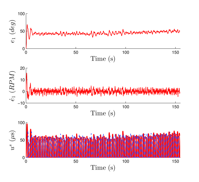
Figure 2: Tracking performance and input of the switched FES-cycling controller.

Note that the error is ultimately bounded and that the control input switches between muscle groups without overlap according to the stimulation regions defined in (2). Fig. 3 illustrates the switching behavior of the control input in (3)

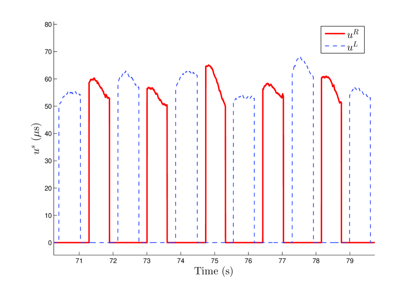
Figure 3: Switched control input $u^{s}$ over a subset of the total experiment runtime illustrating the switching behavior of the controller.

VI Conclusion

An FES-cycling stimulation pattern for the human quadriceps femoris muscle groups is derived from torque transfer ratios which define the effectiveness of knee torques at producing positive torque about a stationary cycle’s crank. The design of the stimulation pattern allows for arbitrary resizing of the stimulation regions through choice of the constant $\varepsilon$, provided they have nonzero length and do not contain the cycling dead points. The results of [8] suggest that $\varepsilon$ should be made as large as possible to minimize the stimulation region while maximizing stimulation intensity for optimal metabolic efficiency.

Since the controller switches between muscle groups based on the state-dependent stimulation pattern and there exist regions where no control is applied, the resulting system is a switched system with autonomous state-dependent switching which must satisfy a reverse dwell-time condition (RDT). The nonlinear nature of the system along with parametric uncertainty and the presence of an unknown bounded disturbance make the RDT condition uncertain, so a switched sliding-mode controller is designed and Lyapunov methods for switched systems are utilized to develop sufficient conditions on the control gains and the desired trajectory which ensure the RDT condition is satisfied. Specifically, if the desired trajectory is designed to satisfy (37) and (42), then (27) is satisfied and the result of Theorem 3 follows. Note that (42) only restricts the desired trajectory at the off-times, giving freedom to design the desired trajectory everywhere else, provided $q_{d}$ and $\dot{q}_{d}$ are continuously differentiable and that the maximum value of $\dot{q}_{d}$ satisfies (37).

The switched controller guarantees ultimately bounded tracking in the sense that the norm of the error vector, $\left\|z\left(t\right)\right\|,$ converges to a ball of constant radius $d,$ and experimental results are provided which demonstrate the performance of the controller. The size of the ultimate bound depends on $\varepsilon$, the control gains, and the system parameters. The stimulation pattern and switched controller may enable improved efficiency and power output in FES-cycling systems. Future work will focus on further experimental verification of this control strategy, its effect on efficiency and power output, and stimulation of additional muscle groups.

References

- [1] C. A. Phillips, J. S. Petrofsky, D. M. Hendershot, and D. Stafford, “Functional electrical exercise: A comprehensive approach for physical conditioning of the spinal cord injured patient,” Orthopedics, vol. 7, no. 7, pp. 1112–1123, 1984.
- [2] C.-W. Peng, S.-C. Chen, C.-H. Lai, C.-J. Chen, C.-C. Chen, J. Mizrahi, and Y. Handa, “Review: Clinical benefits of functional electrical stimulation cycling exercise for subjects with central neurological impairments,” J. Med. Biol. Eng., vol. 31, pp. 1–11, 2011.
- [3] K. J. Hunt, J. Fang, J. Saengsuwan, M. Grob, and M. Laubacher, “On the efficiency of FES cycling: A framework and systematic review,” Technol. Health Care, vol. 20, no. 5, pp. 395–422, 2012.
- [4] K. J. Hunt, D. Hosmann, M. Grob, and J. Saengsuwan, “Metabolic efficiency of volitional and electrically stimulated cycling in able-bodied subjects,” Med. Eng. Phys., vol. 35, no. 7, pp. 919–925, July 2013.
- [5] J. Szecsi, P. Krause, S. Krafczyk, T. Brandt, and A. Straube, “Functional output improvement in FES cycling by means of forced smooth pedaling,” Med. Sci. Sports Exerc., vol. 39, no. 5, pp. 764–780, May 2007.
- [6] B. S. K. K. Ibrahim, S. C. Gharooni, M. O. Tokhi, and R. Massoud, “Energy-efficient FES cycling with quadriceps stimulation,” in Proc. 13th Ann. Conf. of the Int. Funct. Electrical Stimulation Soc., Freiburg, Germany, September 2008.
- [7] M. Gföhler and P. Lugner, “Cycling by means of functional electrical stimulation,” IEEE Trans. Rehabil. Eng., vol. 8, no. 2, pp. 233–243, 2000.
- [8] E. S. Idsø, T. Johansen, and K. J. Hunt, “Finding the metabolically optimal stimulation pattern for FES-cycling,” in Proc. 9th Ann. Conf. of the Int. Funct. Electrical Stimulation Soc., Bournemouth, UK, September 2004.
- [9] R. D. Trumbower and P. D. Faghri, “Improving pedal power during semireclined leg cycling,” IEEE Eng. Med. Biol., vol. 23, no. 2, pp. 62–71, March-April 2004.
- [10] K. J. Hunt, C. Ferrario, S. Grant, B. Stone, A. N. McLean, M. H. Fraser, and D. B. Allan, “Comparison of stimulation patterns for FES-cycling using measures of oxygen cost and stimulation cost,” Med. Eng. Phys., vol. 28, no. 7, pp. 710–718, September 2006.
- [11] N. A. Hakansson and M. L. Hull, “Muscle stimulation waveform timing patterns for upper and lower leg muscle groups to increase muscular endurance in functional electrical stimulation pedaling using a forward dynamic model,” IEEE Trans. Biomed. Eng., vol. 56, no. 9, pp. 2263–2270, September 2009.
- [12] T. A. Perkins, N. N. Donaldson, N. A. C. Hatcher, I. D. Swain, and D. E. Wood, “Control of leg-powered paraplegic cycling using stimulation of the lumbro-sacral anterior spinal nerve roots,” IEEE Trans. Neur. Sys. and Rehab. Eng., vol. 10, no. 3, pp. 158–164, September 2002.
- [13] P. C. Eser, N. Donaldson, H. Knecht, and E. Stussi, “Influence of different stimulation frequencies on power output and fatigue during FES-cycling in recently injured SCI people,” IEEE Trans. Neur. Sys. and Rehab. Eng., vol. 11, no. 3, pp. 236–240, September 2003.
- [14] M. Decker, L. Griffin, L. Abraham, and L. Brandt, “Alternating stimulation of synergistic muscles during functional electrical stimulation cycling improves endurance in persons with spinal cord injury,” J. Electromyogr. Kinesiol., vol. 20, no. 6, pp. 1163 – 1169, 2010.
- [15] N. A. Hakansson and M. L. Hull, “Can the efficacy of eletrically stimulated pedaling using a commercially available ergometer be improved by minimizing the muscle stress-time integral?” Muscle Nerve, vol. 45, no. 3, pp. 393–402, March 2012.
- [16] K. J. Hunt, B. Stone, N.-O. Negård, T. Schauer, M. H. Fraser, A. J. Cathcart, C. Ferrario, S. A. Ward, and S. Grant, “Control strategies for integration of electric motor assist and functional electrical stimulation in paraplegic cycling: Utility for exercise testing and mobile cycling,” IEEE Trans. Neur. Sys. and Rehab. Eng., vol. 12, no. 1, pp. 89–101, March 2004.
- [17] J.-J. J. Chen, N.-Y. Yu, D.-G. Huang, B.-T. Ann, and G.-C. Chang, “Applying fuzzy logic to control cycling movement induced by functional electrical stimulation,” IEEE Trans. Neur. Sys. and Rehab. Eng., vol. 5, no. 2, pp. 158–169, June 1997.
- [18] C.-S. Kim, G.-M. Eom, K. Hase, G. Khang, G.-R. Tack, J.-H. Yi, and J.-H. Jun, “Stimulation pattern-free control of FES cycling: Simulation study,” IEEE Trans. Syst. Man Cybern. Part C Appl. Rev., vol. 38, no. 1, pp. 125–134, January 2008.
- [19] A. Farhoud and A. Erfanian, “Fully automatic control of paraplegic FES pedaling using higher-order sliding mode and fuzzy logic control,” IEEE Trans. Neur. Sys. and Rehab. Eng., vol. PP, no. 99, p. 1, January 2014.
- [20] D. J. Pons, C. L. Vaughan, and G. G. Jaros, “Cycling device powered by the electrically stimulated muscles of paraplegics,” Med. Biol. Eng. Comput., vol. 27, pp. 1–7, 1989.
- [21] J. S. Petrofsky, “New algorithm to control a cycle ergometer using electrical stimulation,” Med. Biol. Eng. Comput., vol. 41, no. 1, pp. 18–27, January 2003.
- [22] D. Liberzon, Switching in Systems and Control. Birkhauser, 2003.
- [23] J. P. Hespanha, D. Liberzon, and A. R. Teel, “Lyapunov conditions for input-to-state stability of implusive systems,” Automatica, vol. 44, no. 11, pp. 2735–2744, November 2008.
- [24] E. S. Idsø, “Development of a mathematical model of a rider-tricycle system,” Dept. of Engineering Cybernetics, NTNU, Tech. Rep., 2002.
- [25] L. M. Schutte, M. M. Rodgers, F. E. Zajac, and R. M. Glaser, “Improving the efficacy of electrical stimulation-induced leg cycle ergometry: An analysis based on a dynamic musculoskeletal model,” IEEE Trans. Rehabil. Eng., vol. 1, no. 2, pp. 109–125, 1993.
- [26] N. Sharma, K. Stegath, C. M. Gregory, and W. E. Dixon, “Nonlinear neuromuscular electrical stimulation tracking control of a human limb,” IEEE Trans. Neural Syst. Rehabil. Eng., vol. 17, no. 6, pp. 576–584, 2009.
- [27] M. Ferrarin and A. Pedotti, “The relationship between electrical stimulus and joint torque: A dynamic model,” IEEE Trans. Rehabil. Eng., vol. 8, no. 3, pp. 342–352, 2000.
- [28] T. Schauer, N. O. Negard, F. Previdi, K. J. Hunt, M. H. Fraser, E. Ferchland, and J. Raisch, “Online identification and nonlinear control of the electrically stimulated quadriceps muscle,” Control Eng. Pract., vol. 13, pp. 1207–1219, 2005.
- [29] A. Filippov, “Differential equations with discontinuous right-hand side,” Am. Math. Soc. Transl., vol. 42 no. 2, pp. 199–231, 1964.
- [30] B. Paden and S. Sastry, “A calculus for computing Filippov’s differential inclusion with application to the variable structure control of robot manipulators,” IEEE Trans. Circuits Syst., vol. 34 no. 1, pp. 73–82, 1987.
- [31] G.-C. Chang, J.-J. Lub, G.-D. Liao, J.-S. Lai, C.-K. Cheng, B.-L. Kuo, and T.-S. Kuo, “A neuro-control system for the knee joint position control with quadriceps stimulation,” IEEE Trans. Rehabil. Eng., vol. 5, no. 1, pp. 2–11, Mar. 1997.
- [32] K. Kurosawa, R. Futami, T. Watanabe, and N. Hoshimiya, “Joint angle control by FES using a feedback error learning controller,” IEEE Trans. Neural Syst. Rehabil. Eng., vol. 13, pp. 359–371, 2005.
- [33] S. Jezernik, R. Wassink, and T. Keller, “Sliding mode closed-loop control of FES: Controlling the shank movement,” IEEE Trans. Biomed. Eng., vol. 51, pp. 263–272, 2004.
- [34] J. Hausdorff and W. Durfee, “Open-loop position control of the knee joint using electrical stimulation of the quadriceps and hamstrings,” Med. Biol. Eng. Comput., vol. 29, pp. 269–280, 1991.