DPF2013-45 September 30, 2013

Measurements of $B\rightarrow DK$ decays to constrain the CKM Unitarity Triangle angle $\gamma$ and related results at LHCb

Daniel Craik

Department of Physics
University of Warwick, Coventry, UK

Constraints on the CKM angle $\gamma$ are presented from GLW, ADS, and GGSZ analyses of $B^{\pm}\rightarrow DK^{\pm}$ at the LHCb experiment. The branching fractions of $B^{0}\rightarrow\overline{D}^{0}K^{+}\pi^{-}$ and $B_{s}^{0}\rightarrow\overline{D}^{0}K^{-}\pi^{+}$ are also reported, measured relative to the related mode $B^{0}\rightarrow\overline{D}^{0}\pi^{+}\pi^{-}$.

PRESENTED AT

DPF 2013
The Meeting of the American Physical Society
Division of Particles and Fields
Santa Cruz, California, August 13–17, 2013

1 Measurements of $\gamma$ from $B^{\pm}\rightarrow DK^{\pm}$

The CKM angle $\gamma=\text{arg}(-V_{\text{ud}}V^{*}_{\text{ub}}/V_{\text{cd}}V^{*}_{\text{cb}})$ is currently the least well-constrained angle in the Unitarity Triangle. So far, the most-sensitive measurements of $\gamma$ from a single experiment have been performed by Belle [1] and BaBar [2]. These measurements yield values of $\left(68^{+15}_{-14}\right)^{\circ}$ and $\left(69^{+17}_{-16}\right)^{\circ}$, respectively.

Tree-level processes such as $B^{\pm}\rightarrow DK^{\pm}$ provide a theoretically clean measurement of $\gamma$ with no contributions from new physics processes. This measurement can be compared with measurements from loop-mediated processes, which are sensitive to new physics, to provide a test of the Standard Model. The current limits on the CKM Unitarity Triangle due to tree-level and loop processes, as calculated by the CKMFitter group [3], are shown in Fig. 1.

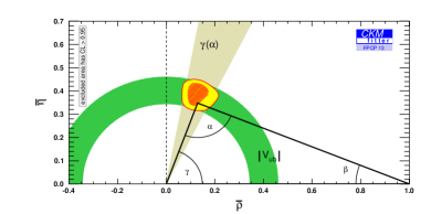
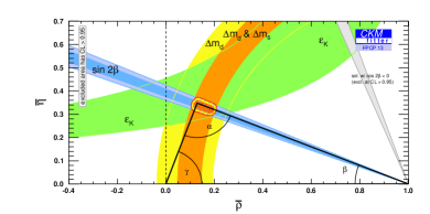
Figure 1: Constraints on the CKM Unitarity Triangle due to (left) tree-level processes and (right) loop-mediated processes.

1.1 GLW/ADS analysis of $B^{\pm}\rightarrow DK^{\pm}$ and $B^{\pm}\rightarrow D\pi^{\pm}$

The GLW method [4] uses $D$ decays to $C\!P$ eigenstates such as $K^{+}K^{-}$ and $\pi^{+}\pi^{-}$. Decays can proceed either via a $D^{0}$ or a $\overline{D}^{0}$ with a phase difference of $\delta_{B}+\gamma$. Suppression in the decay via $D^{0}$ with respect to the $\overline{D}^{0}$ decay limits interference to $\mathcal{O}(10\,\%)$ in $B^{\pm}\rightarrow DK^{\pm}$ and $\mathcal{O}(1\,\%)$ in $B^{\pm}\rightarrow D\pi^{\pm}$.

The ADS method [5] uses $D$ decays to quasi-flavour-specific states such as $\pi^{+}K^{-}$ and $\pi^{-}K^{+}\pi^{+}\pi^{-}$. Here the suppression of one of the $B$ decays is partially balanced by the suppression of one of the $D$ decays, giving larger interference terms while also introducing an additional phase shift of $\delta_{D}$.

Analyses have been performed on $B^{\pm}\rightarrow DK^{\pm}$ and $B^{\pm}\rightarrow D\pi^{\pm}$ with the $D$ meson reconstructed from the final states $K^{+}K^{-}$, $\pi^{+}\pi^{-}$, $K^{+}\pi^{-}$, $\pi^{+}K^{-}$, $K^{-}\pi^{+}\pi^{+}\pi^{-}$ and $\pi^{-}K^{+}\pi^{+}\pi^{-}$ using LHCb data corresponding to $1\,\text{fb}^{-1}$ of $pp$ collisions at a centre of mass energy of 7 TeV [6, 7]. The invariant mass distributions of the two- and four-body suppressed ADS modes are shown in Fig. 2 and Fig. 3, respectively.

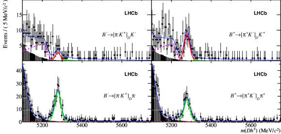
Figure 2: Fits to the invariant mass distributions of the two-body suppressed ADS mode $\pi^{\mp}K^{\pm}$ in (top) $B^{\mp}\rightarrow DK^{\mp}$ and (bottom) $B^{\mp}\rightarrow D\pi^{\mp}$. The $B^{\mp}\rightarrow DK^{\mp}$ and $B^{\mp}\rightarrow D\pi^{\mp}$ components are shown in red and green, respectively. The shaded component indicates partially reconstructed backgrond, the dashed magenta line corresponds to partially reconstructed $\Lambda_{b}^{0}\rightarrow\Lambda_{c}^{+}h^{-}$ and the total shape also includes a combinatoric background.

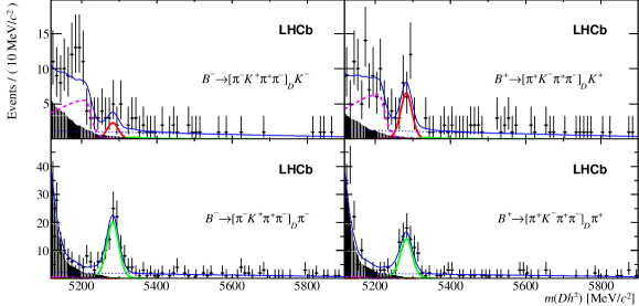
Figure 3: Fits to the invariant mass distributions of the four-body suppressed ADS mode $\pi^{\mp}K^{\pm}\pi^{\pm}\pi^{\mp}$ in (top) $B^{\mp}\rightarrow DK^{\mp}$ and (bottom) $B^{\mp}\rightarrow D\pi^{\mp}$. The $B^{\mp}\rightarrow DK^{\mp}$ and $B^{\mp}\rightarrow D\pi^{\mp}$ components are shown in red and green, respectively. The shaded component indicates partially reconstructed backgrond, the dashed magenta line corresponds to partially reconstructed $B_{s}^{0}\rightarrow DK^{-}\pi^{+}$ and the total shape also includes a combinatoric background.

The observables measured are the ratio of $DK$ to $D\pi$ for each $D$ final state,

$$R_{K/\pi}^{f}=\frac{\Gamma\left(B^{-}\rightarrow D\left[\rightarrow f\right]K^{-}\right)+\Gamma\left(B^{+}\rightarrow D\left[\rightarrow\overline{f}\right]K^{+}\right)}{\Gamma\left(B^{-}\rightarrow D\left[\rightarrow f\right]\pi^{-}\right)+\Gamma\left(B^{+}\rightarrow D\left[\rightarrow\overline{f}\right]\pi^{+}\right)}\,,$$

the charge asymmetry for each final state,

$$A_{h}^{f}=\frac{\Gamma\left(B^{-}\rightarrow D\left[\rightarrow f\right]h^{-}\right)-\Gamma\left(B^{+}\rightarrow D\left[\rightarrow\overline{f}\right]h^{+}\right)}{\Gamma\left(B^{-}\rightarrow D\left[\rightarrow f\right]h^{-}\right)+\Gamma\left(B^{+}\rightarrow D\left[\rightarrow\overline{f}\right]h^{+}\right)}\,,$$

and the ratio of the suppressed to favoured modes for $D\rightarrow K\pi$ and $D\rightarrow K\pi\pi\pi$,

$$R_{h}^{\pm}=\frac{B^{\pm}\rightarrow D\left[f_{\text{sup}}\right]h^{\pm}}{B^{\pm}\rightarrow D\left[f\right]h^{\pm}}\,.$$

The values obtained for each of these observables can be found in Refs. [6, 7]. These variables serve as inputs for the combined $\gamma$ measurements in Section 1.3 and Section 1.4.

1.2 GGSZ analysis of $B^{\pm}\rightarrow DK^{\pm}$

The GGSZ method [8] exploits the variation of the strong phase $\delta_{D}$ across the Dalitz plot in $D$ decays to three-body self-conjugate states such as $K_{S}^{0}\pi^{+}\pi^{-}$ and $K_{S}^{0}K^{+}K^{-}$. The Dalitz plot is divided into bins, as shown in Fig. 4, chosen to maximise statistical sensitivity. The populations of $B^{+}$ and $B^{-}$ decays in each bin are given by

$$N^{+}_{\pm i}=h_{B^{+}}\left[K_{\mp i}+(x^{2}_{+}+y^{2}_{+})K_{\pm i}+2\sqrt{K_{i}K_{-i}}(x_{+}c_{\pm i}\mp y_{+}s_{\pm i})\right]\,,$$

$$N^{-}_{\pm i}=h_{B^{-}}\left[K_{\pm i}+(x^{2}_{-}+y^{2}_{-})K_{\mp i}+2\sqrt{K_{i}K_{-i}}(x_{-}c_{\pm i}\pm y_{-}s_{\pm i})\right]\,,$$

where $K_{\pm i}$ is the efficiency corrected yield in bin $\pm i$ due to $D^{0}$ flavour tagged events from BaBar [9, 10] and $c_{\pm i}$ and $s_{\pm i}$ are the cosine and sine of the strong phase $\delta_{D}$ in bin $\pm i$ from CLEO-c [11].

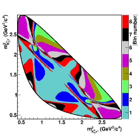
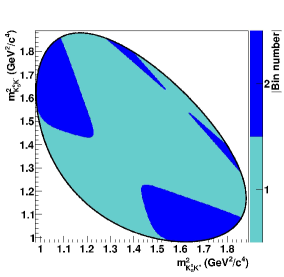
Figure 4: Binning schemes used for the Dalitz plots of (left) $D\rightarrow K_{S}^{0}\pi^{+}\pi^{-}$ and (right) $D\rightarrow K_{S}^{0}K^{+}K^{-}$. Bins in the top-left half of the plots ($m^{2}_{K_{S}^{0}h^{-}}>m^{2}_{K_{S}^{0}h^{+}}$) are identified as $+i$ and bins in the bottom-right half are labeled $-i$.

The remaining parameters are left free in the fit to the data: $h_{B^{\pm}}$ are normalisation factors for $B^{\pm}$, and $x_{\pm}=r_{B}\text{cos}(\delta_{B}\pm\gamma)$ and $y_{\pm}=r_{B}\text{sin}(\delta_{B}\pm\gamma)$ are the Cartesian parameters, which are sensitive to $\gamma$.

Analyses have been performed on $B^{\pm}\rightarrow DK^{\pm}$ with the $D$ meson reconstructed in the final states $K_{S}^{0}\pi^{+}\pi^{-}$ and $K_{S}^{0}K^{+}K^{-}$ using LHCb data corresponding to $1\,\text{fb}^{-1}$ of $pp$ collisions at a centre of mass energy of 7 TeV [12] and $2\,\text{fb}^{-1}$ of $pp$ collisions at a centre of mass energy of 8 TeV [13]. The values obtained for the Cartesian parameters in the 8 TeV analysis are

$$x_{+}=\left(-8.7\pm 3.1\text{(stat.)}\pm 1.6\text{(syst.)}\pm 0.6\text{(ext.)}\right)\times 10^{-2}\,,$$

$$x_{-}=\left(\phantom{-}5.3\pm 3.2\text{(stat.)}\pm 0.9\text{(syst.)}\pm 0.9\text{(ext.)}\right)\times 10^{-2}\,,$$

$$y_{+}=\left(\phantom{-}0.1\pm 3.6\text{(stat.)}\pm 1.4\text{(syst.)}\pm 1.9\text{(ext.)}\right)\times 10^{-2}\,,$$

$$y_{-}=\left(\phantom{-}9.9\pm 3.6\text{(stat.)}\pm 2.2\text{(syst.)}\pm 1.6\text{(ext.)}\right)\times 10^{-2}\,,$$

where the third uncertainty is due to the CLEO-c strong phase measurements used in the fit.

Combining these values with the results from the 7 TeV analysis and fitting for $\gamma$, $r_{B}$ and $\delta_{B}$ yields values of $(57\pm 16)^{\circ}$, $(8.8^{+2.3}_{-2.4})\times 10^{-2}$ and $(124^{+15}_{-17})^{\circ}$, respectively, where the values for $\gamma$ and $\delta_{B}$ are modulo $180^{\circ}$. Two-dimensional projections of the confidence regions for these parameters are shown in Fig. 5.

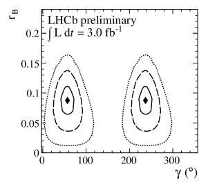
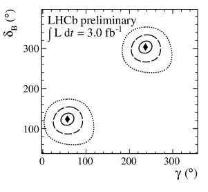
Figure 5: Two-dimensional projections of the confidence regions onto the (left) $(\gamma,r_{B})$ and (right) $(\gamma,\delta_{B})$ planes. Contours indicate the $1$, $2$ and $3\sigma$ boundaries and diamonds mark the central values.

1.3 Combination of results from $1\,\text{fb}^{-1}$ measurements

The results in Section 1.1 and Section 1.2 are combined using a frequentist approach to obtain a more constraining measurement of $\gamma$  [14]. In addition to these results further measurements are included to improve the fit: measurements of the strong phases and coherence factors for $D\rightarrow K\pi$ and $D\rightarrow K\pi\pi\pi$ decays from CLEO-c[15], $C\!P$ asymmetry measurements of the neutral $D$ mesons from the Heavy Flavour Averaging Group[16] and charm mixing parameters from LHCb[17]. A likelihood is constructed from the measured observables as

$${\cal L}\left(\vec{\alpha}\right)={\displaystyle\prod_{i}}\xi_{i}\left(\vec{A}_{i}^{\text{obs}}|\vec{\alpha}\right)\,,$$

where the sum is over the different measurements, $\vec{\alpha}$ is the set of parameters and $\xi_{i}$ denotes the likelihood probability density functions (PDFs) of the observables $\vec{A}_{i}^{\text{obs}}$. For most observables a Gaussian PDF is assumed, however, where highly non-Gaussian behaviour is observed, the experimental likelihood is used.

A combined $\gamma$ measurement has been performed including the results from Section 1.1 and a subset of the results from Section 1.2 corresponding to $1\,\text{fb}^{-1}$ of $pp$ collisions at a centre of mass energy of 7 TeV [12]. The best-fit values and confidence intervals (modulo $180^{\circ}$) of $\gamma$ are given in Table 1 and the $1-\text{CL}$ curves for $\gamma$ are shown in Fig. 6.

combination	$\gamma$	68 % CL	95 % CL
$DK$	$72.0^{\circ}$	$[56.4,86.7]^{\circ}$	$[42.6,99.6]^{\circ}$
$D\pi$	$18.9^{\circ}$	$[7.4,99.2]^{\circ}\cup[167.9,176.4]^{\circ}$	-
$DK$ and $D\pi$	$72.6^{\circ}$	$[55.4,82.3]^{\circ}$	$[40.2,92.7]^{\circ}$

Table 1: Best-fit values and confidence intervals for $\gamma$ from the combination of $DK$ and $D\pi$ measurements.

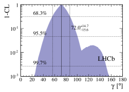
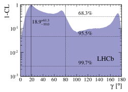
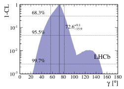
Figure 6: $1-\text{CL}$ curves for $\gamma$ from the combined $1\,\text{fb}^{-1}$ GLW/ADS and $1\,\text{fb}^{-1}$ GGSZ measurements using (left) only $DK$, (centre) only $D\pi$ and (right) both decay modes.

1.4 Combination including $3\,\text{fb}^{-1}$ GGSZ measurement

Another combination [18] has been performed that incorporates all of the results reported in Section 1.2 but only those observables from Section 1.1 corresponding to $B^{\pm}\rightarrow DK^{\pm}$ decays. Mixing in the neutral $D$ mesons is also neglected in the equations used for the observables in this combination.

The best-fit values and confidence intervals (all modulo $180^{\circ}$) for $\gamma$, $r_{B}$ and $\delta_{B}$ are given in Table 2. Figure 7 and Figure 8 show the $1-\text{CL}$ curve for $\gamma$, and the 2D projection of the likelihood in $\gamma$ and $r_{B}$, respectively.

quantity	value	68 % CL	95 % CL
$\gamma$	$67.2^{\circ}$	$[55.1,79.1]^{\circ}$	$[43.9,89.5]^{\circ}$
$r_{B}$	$0.0923$	$[0.0843,0.1001]$	$[0.0762,0.1075]$
$\delta_{B}$	$114.3^{\circ}$	$[101.3,126.3]^{\circ}$	$[88.7,136.3]^{\circ}$

Table 2: Best-fit values and confidence intervals for $\gamma$, $r_{B}$ and $\delta_{B}$ from the combination of $DK$ measurements including GGSZ measurements from $3\,\text{fb}^{-1}$ of data.

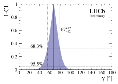
Figure 7: $1-\text{CL}$ curve for $\gamma$ from the combined $1\,\text{fb}^{-1}$ GLW/ADS and $3\,\text{fb}^{-1}$ GGSZ measurements.

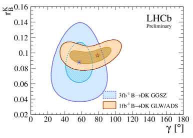
Figure 8: Two-dimensional projection of the confidence regions onto the $(\gamma,r_{B})$ plane. Contours show the $1$ and $2\sigma$ boundaries and markers indicate the central values.

2 Measurement of $B_{(s)}^{0}\rightarrow DK\pi$ branching fractions

The decay mode $B^{0}\rightarrow DK^{+}\pi^{-}$ has potential for a significant future measurement of $\gamma$ [19, 20, 21]. Sensitivity to $\gamma$ comes from the interference of $b\rightarrow c$ and $b\rightarrow u$ amplitudes of a similar magnitude. $B_{s}^{0}\rightarrow DK^{-}\pi^{+}$ and the related mode $B_{s}^{0}\rightarrow D^{*}K^{-}\pi^{+}$ form important backgrounds to this mode, therefore, an understanding of these modes is necessary.

Branching fraction measurements of $B^{0}\rightarrow DK^{+}\pi^{-}$ and $B_{s}^{0}\rightarrow DK^{-}\pi^{+}$, relative to the normalisation mode $B^{0}\rightarrow D\pi^{+}\pi^{-}$, have been made using LHCb data corresponding to $1\,\text{fb}^{-1}$ of $pp$ collisions at a centre of mass energy of 7 TeV [22]. The invariant mass distributions of $D\pi\pi$ and $DK\pi$ candidates where the $D$ is reconstructed from $\overline{D}^{0}\rightarrow K^{+}\pi^{-}$ are shown in Fig. 9. The measured relative branching fractions are

$$\frac{{\cal B}\left(B^{0}\to\overline{D}^{0}K^{+}\pi^{-}\right)}{{\cal B}\left(B^{0}\to\overline{D}^{0}\pi^{+}\pi^{-}\right)}=0.106\pm 0.007\,\text{(stat.)}\pm 0.008\,\text{(syst.)}\,,$$

$$\frac{{\cal B}\left(B_{s}^{0}\to\overline{D}^{0}K^{-}\pi^{+}\right)}{{\cal B}\left(B^{0}\to\overline{D}^{0}\pi^{+}\pi^{-}\right)}=1.18\pm 0.05\,\text{(stat.)}\pm 0.12\,\text{(syst.)}\,.$$

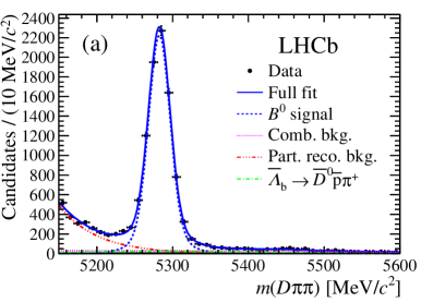
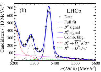
Figure 9: Fits to the $B^{0}_{(s)}$ candidate invariant mass distributions for the (a) $D\pi\pi$ and (b) $DK\pi$ samples. Data points are shown in black, the full fitted PDFs as solid blue lines and the components as detailed in the legends.

These relative measurements yield absolute branching fractions of

$${\cal B}\left(B^{0}\to\overline{D}^{0}K^{+}\pi^{-}\right)=(9.0\pm 0.6\,\text{(stat.)}\pm 0.7\,\text{(syst.)}\pm 0.9({\cal B}))\times 10^{-5}\,,$$

$${\cal B}\left(B_{s}^{0}\to\overline{D}^{0}K^{-}\pi^{+}\right)=(1.00\pm 0.04\,\text{(stat.)}\pm 0.10\,\text{(syst.)}\pm 0.10({\cal B}))\times 10^{-3}\,,$$

where the third uncertainty arises from the uncertainties on ${\cal B}(B^{0}\to\overline{D}^{0}\pi^{+}\pi^{-})$. This is the most precise measurement of ${\cal B}(B^{0}\to\overline{D}^{0}K^{+}\pi^{-})$ to date and the first measurement of ${\cal B}(B_{s}^{0}\to\overline{D}^{0}K^{-}\pi^{+})$.

Although no quantitative analysis of the Dalitz plots has yet been attempted, the Dalitz plot distributions obtained (corrected for efficiency) are presented in Fig. 10.

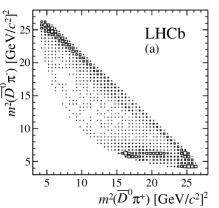
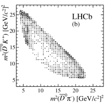
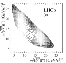
Figure 10: Efficiency corrected Dalitz plot distributions for (a) $B^{0}\rightarrow\overline{D}^{0}\pi^{+}\pi^{-}$, (b) $B^{0}\rightarrow\overline{D}^{0}K^{+}\pi^{-}$ and (c) $B_{s}^{0}\rightarrow\overline{D}^{0}K^{-}\pi^{+}$ candidates obtained from the signal weights.

3 Conclusions and prospects

The $B^{\pm}\rightarrow DK^{\pm}$ decay mode offers an excellent opportunity to measure the CKM angle $\gamma$ from Standard Model processes. The combination in Section 1.4 gives the most sensitive measurement of $\gamma$ from a single experiment so far, yielding a value of $(67\pm 12)^{\circ}$. This measurement is expected to improve further with the completion of a GLW/ADS analysis on the remaining $2\,\text{fb}^{-1}$ of LHCb data currently available. In addition, other modes such as $B^{0}\rightarrow DK^{+}\pi^{-}$ offer great prospects for future $\gamma$ measurements.

ACKNOWLEDGMENTS

This work is funded in part by the European Research Council under FP7 and by the United Kingdom’s Science and Technology Facilities Council.

References

- [1] K. Trabelsi [Belle Collaboration], arXiv:1301.2033 [hep-ex].
- [2] J. P. Lees et al. [BaBar Collaboration], Phys. Rev. D 87 (2013) 052015 [arXiv:1301.1029 [hep-ex]].
- [3] J. Charles et al. [CKMfitter Group Collaboration], Eur. Phys. J. C 41 (2005) 1 [hep-ph/0406184].
- [4] M. Gronau and D. Wyler, Phys. Lett. B 265 (1991) 172.
- [5] D. Atwood, I. Dunietz and A. Soni, Phys. Rev. Lett. 78 (1997) 3257 [hep-ph/9612433].
- [6] R. Aaij et al. [LHCb Collaboration], Phys. Lett. B 712 (2012) 203 [Erratum-ibid. B 713 (2012) 351] [arXiv:1203.3662 [hep-ex]].
- [7] R. Aaij et al. [LHCb Collaboration], Phys. Lett. B 723 (2013) 44 [arXiv:1303.4646 [hep-ex]].
- [8] A. Giri, Y. Grossman, A. Soffer and J. Zupan, Phys. Rev. D 68 (2003) 054018 [hep-ph/0303187].
- [9] B. Aubert et al. [BaBar Collaboration], Phys. Rev. D 78 (2008) 034023 [arXiv:0804.2089 [hep-ex]].
- [10] P. del Amo Sanchez et al. [BaBar Collaboration], Phys. Rev. Lett. 105 (2010) 121801 [arXiv:1005.1096 [hep-ex]].
- [11] J. Libby et al. [CLEO Collaboration], Phys. Rev. D 82 (2010) 112006 [arXiv:1010.2817 [hep-ex]].
- [12] R. Aaij et al. [LHCb Collaboration], Phys. Lett. B 718 (2012) 43 [arXiv:1209.5869 [hep-ex]].
- [13] R. Aaij et al. [LHCb Collaboration], LHCb-CONF-2013-004 (2013).
- [14] R. Aaij et al. [LHCb Collaboration], arXiv:1305.2050 [hep-ex].
- [15] N. Lowrey et al. [CLEO Collaboration], Phys. Rev. D 80 (2009) 031105 [arXiv:0903.4853 [hep-ex]].
- [16] Y. Amhis et al. [Heavy Flavor Averaging Group Collaboration], arXiv:1207.1158 [hep-ex].
- [17] R. Aaij et al. [LHCb Collaboration], Phys. Rev. Lett. 110 (2013) 101802 [arXiv:1211.1230 [hep-ex]].
- [18] R. Aaij et al. [LHCb Collaboration], LHCb-CONF-2013-006 (2013).
- [19] M. Gronau, Phys. Lett. B 557 (2003) 198 [hep-ph/0211282].
- [20] T. Gershon, Phys. Rev. D 79 (2009) 051301 [arXiv:0810.2706 [hep-ph]].
- [21] T. Gershon and M. Williams, Phys. Rev. D 80 (2009) 092002 [arXiv:0909.1495 [hep-ph]].
- [22] R. Aaij et al. [LHCb Collaboration], Phys. Rev. D 87 (2013) 112009 [arXiv:1304.6317 [hep-ex]].