An Image-Based Fluid Surface Pattern Model

Abstract

This work aims at generating a model of the ocean surface and its motion from one or more video cameras. The idea is to model wave patterns from video as a first step towards a larger system of photogrammetric monitoring of marine conditions for use in offshore oil drilling platforms. The first part of the proposed approach consists in reducing the dimensionality of sensor data made up of the many pixels of each frame of the input video streams. This enables finding a concise number of most relevant parameters to model the temporal dataset, yielding an efficient data-driven model of the evolution of the observed surface. The second part proposes stochastic modeling to better capture the patterns embedded in the data. One can then draw samples from the final model, which are expected to simulate the behavior of previously observed flow, in order to determine conditions that match new observations. In this paper we focus on proposing and discussing the overall approach and on comparing two different techniques for dimensionality reduction in the first stage: principal component analysis and diffusion maps. Work is underway on the second stage of constructing better stochastic models of fluid surface motion as proposed here.

Keywords: Inverse problems, fluid motion, nonrigid 3D reconstruction, dimensionality reduction, diffusion maps, pattern theory

1 Introduction

The simulation of fluids is an imporant tool in computer graphics, e.g., for generating realistic animations of water flow. Many fluid simulations perform the evolution of liquid through time based on the Navier-Stokes equation or simpler wave and frequency models, among others. This work is an initial part of a larger effort to perform the inverse problem of generating graphics simulations, i.e., to automatically extract 3D models of fluid surfaces starting from real-world video data. The obtained model can then be used for simulating the motion of ocean surface patterns as observed in the real world. Moreover, this simulation can be matched to video at new time instants in order to predict and track the actual conditions of the observed fluid.

In order to track the apparently complex dynamics of a large number of images of the ocean surface, our proposed system reduces the dimensionality of previsouly observed data and automatically learns a concise data-driven model. This enables the inference through synthesis of patterns that are intrisic to the observed phenomenon, while drastically reducing the search space with little to no loss. The remaining error in the low dimensional modeling is dealt with as part of a stochastic modeling stage.

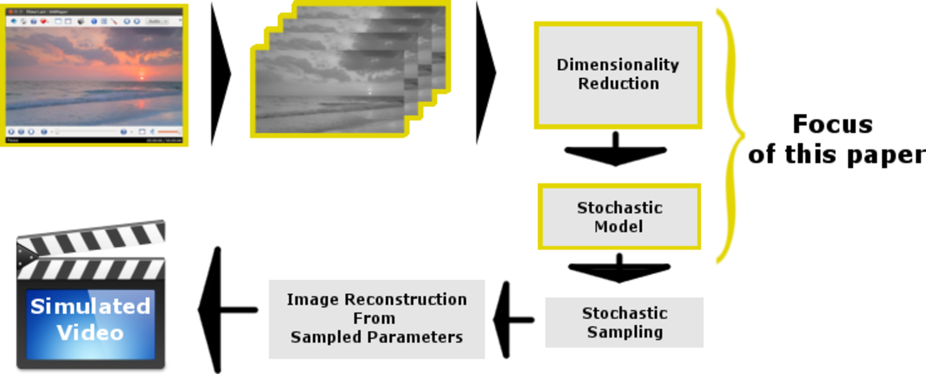
While detailed techniques for the plausible inference involving such patterns is ongoing work, we propose that the patterns in newly observed data are to be found by stochastic modeling, using the Bayesian paradigm, a method which can be described as “analysis by synthesis” (Mumford & Desolneux,, 2010). Finally, a stochastic model also enables generating plausible new images for a realistic image-based simulation. Figure 1 shows a diagram representing the steps of the proposed modeling approach dealt with in this manuscript.

Two dimensionality reduction techniques were assessed: (i) principal components analysis, which consists in performing orthogonal projections of data along linear directions of greater variance; and (ii) diffusion maps, a recent non-linear technique which organizes data into graphs of local similarity and extracts global structure through a diffusion process (Lafon & Lee,, 2006).

Figure 1: Diagram of the proposed approach for the modeling of fluid surface patterns aiming at applications of monitoring ocean conditions for offshore oil drilling processes, among others.

2 Dimensionality Reduction Techniques

Assume a video is made up of $n$ video frames represented by a column vector $y_{i}$, $i=1,\dots,n$. Each video frame is an image with a total of $p$ pixels, so that each observation or data point is a $p$-dimensional vector $y_{i}\in\mathbbm{R}^{p}$. For instance, frames of a typical high-definition video $1920\times 1080$ are each comprised of more than 2 milion dimensions, an excessive number of parameters to capture the observable modes of variation of fluid surface patterns that are relevant for monitoring applications. We explore two different techniques for automatically reducing this number of parameters as a step towards generating a tractable yet meaningful model.

2.1 Principal Component Analysis

The principal component analysis (PCA) is a linear dimentionality reduction technique. High-dimensional data, i.e., $p$-dimensional, gets reduced by PCA to a global linear submanifold of reduced dimension $q\ll p$, determined by the directions of greatest variability in the data. These directions are given by $q$ orthonormal vectors, the principal components, which are the eigenvectors corresponding to the largest eigenvalues of the covariance matrix of the data.

Principal component analysis can be computed through the singular value decomposition (SVD) (Hastie & et al.,, 2013; Jolliffe,, 2002; Golub & Van Loan,, 1996) as follows. The $n$ observations $y_{i}\in\mathbbm{R}^{p}$ are mean-centered by subtracting their average $\bar{y}=\dfrac{1}{n}\sum^{n}_{j=1}y_{j}$. The new data vectors $x_{i}=y_{i}-\bar{y}$ form the columns of the $p\times n$ data matrix $X$ whose singluar value decomposition is given by

$$X=U\Sigma V^{\top},$$ (1)

with $U$ and $V$ being $p\times n$ and $n\times n$ orthonormal matrices, resp., and $\Sigma$ an $n\times n$ diagonal matrix, with diagonal elements $\sigma_{1}\geq\dots\geq\sigma_{n}\geq 0$ known as singular values. The first $q$ columns of $U$ form the $p\times q$ matrix $U_{q}$, the so-called first $q$ principal components, and $\alpha_{i}=U_{q}\top x_{i}$ are the coordinates of any given observation $x_{i}$ in the subspace of the principal components.

The computation of PCA using SVD is equivalent to computing the eigenvalues and eigenvectors of the covariance matrix, which is given by

$$\dfrac{1}{n-1}XX^{\top}.$$ (2)

It is possible to show this fact by taking the SVD of the matrix $X$ as shown in (1), and building the product $XX^{\top}$, giving

$$XX^{\top}=(U\Sigma V^{\top})(V\Sigma U^{\top}).$$ (3)

Since $V$ is an orthogonal matrix, we have

$$XX^{\top}=U\Sigma^{2}U^{\top}.$$ (4)

From Equation (4) we clearly see the correspondence of the SVD and the covariance of the data samples. The singular values of $X$ are the square roots of the eigenvalues of the covariance matrix, and the singular vectors of $X$ are the eigenvectors of the covariance matrix.

2.1.1 Stochastic SVD

In our application, the dataset is very large and in high dimensions, in which case computing the eigenvalues of the data matrix is a key challenge. Recent techniques enable the computation of large matrix decompositions in a robust manner without explicitly forming the entire data matrix in memory (Halko et al.,, 2010, 2011). The key main idea behind these methods is stochasticity.

For the construction of the SVD using stochasticity, a method we refer in this manuscript as stochastic SVD is available (Halko et al.,, 2011) which can be broken in two stages. First, the construction of a subspace with reduced dimension in which to represent the input data in an approximate manner; a matrix is bult in which the columns form a reduced orthonormal basis for the data. Second, the projection of the observations onto that subspace and the subsequent computation of the SVD. Both stages are outlined in Algorithm 1.

Algorithm 1 – Stochastic SVD

Given an ${m\times n}$ matrix $A$, and integers $l$ and $q$, compute an approximate decomposition of $A\approx U\Sigma V^{\top}$, where $U$ and $V$ are orthonormal and $\Sigma$ is a non-negative diagonal matrix.

1:Create an ${n\times l}$ matrix $\Omega$, with independent entries and standard normal distribution.

2:Form $Y=A\Omega$.

3:Perform the $QR$ decomposition of $Y$, $Y=QR$, with $Q$ an $m\times l$ orthonormal matrix.

4:Form $B=Q^{\top}A$.

5:Compute an SVD of the reduced matrix $B=\tilde{U}\Sigma V^{\top}$.

6:Form the otrhonormal matrix $U=Q\tilde{U}$.

The stochastic SVD provides a robust means to perform large-scale matrix decompositions, independently of the intrinisc structure of the data matrix. However, this approach yields an approximate solution whose quality must be assessed in the context of the original application.

In this work, the purpose of the stochastic SVD is to obtain the principal components of a given dataset, i.e., to obtain the singular vectors to the left of an SVD of a data matrix. We know that the obtained vectors form a basis for a subspace, so that its precision can be assessed at each execution of the stochastic SVD. This assessment was done using a distance between subspaces as described in the next section.

2.1.2 Distance between subspaces

Let $F$ and $G$ be subspaces of $\mathbbm{R}^{m}$, with $p=\textsf{Dim}(F)\geq\textsf{Dim}(G)\geq q\geq 1$. The princpal angles, $\theta_{1},\dots,\theta_{q}\in[0,\pi/2]$, between $F$ and $G$ are recursively defined as being real the numbers $\theta_{k}$ such that

$$\cos(\theta_{k})=\max_{u\in F,v\in G}|u^{\top}v|=|u_{k}^{\top}v_{k}|,$$

subject to

$$u^{\top}u=v^{\top}v=1,\qquad u^{\top}u_{i}=v^{\top}v_{i}=0\ ,\qquad i=1,\dots,k-1.$$

The vectors $\{u_{1},\dots,u_{q}\}$ e $\{v_{1},\dots,v_{q}\}$ are the so-called principal vectors between the subspaces $F$ e $G$.

The greatest principal angle is related to the notion of distance between subspaces of the same dimension (Golub & Van Loan,, 1996). Thus, if $p=q$ then $dist(F,G)=\sqrt{1-\cos(\theta_{p})^{2}}$ $=\hskip 2.0pt\mathrm{sen}(\theta_{p})$. In a practical way, if the columns of $Q_{F}\in\mathbbm{R}^{m\times p}$ and those of $Q_{G}\in\mathbbm{R}^{m\times p}$ define orthonormal bases for $F$ and $G$, respectively, the cosine of the greatest principal angle is determined by computing an SVD of the matrix $Q_{F}^{\top}Q_{G}$ and taking the smallest of its singular values. It is important to note that

$$0\leq dist(F,G)\leq 1.$$

The distance will be zero if $F=G$ and one if $F\cap G^{\perp}\neq\{0\}$, with $G^{\perp}$ denoting the orthogonal complement of $G$, i.e., the space of all orthogonal vectors to $G$.

2.2 Diffusion maps

We have explored a more recent non-linear technique for dimensionality reduction and manifold learning, the so-called diffusion maps, which re-organizes the data according to a reduced set of parameters related to the approximate intrinsic geometry of the underlying phenomena (Lafon & Lee,, 2006; de la Porte et al.,, 2008). The reduced set of parametrs are computed from the eigenvalues and eigenvectors of a diffusion operator on data. It is robust to noise and outliers in data, and can be efficiently computed when its application is properly designed.

Consider that the set of $n$ observations $y_{1},\dots,y_{n}\in\mathbbm{R}^{p}$ approximately sample one or more non-linear manifolds, each $y_{i}$ being a vector of all pixels of a video frame, for instance. We describe the diffusion maps algorithm in four steps. The first step consists in building an $n\times n$ matrix $W$ of pairwise (local) similarities between the observations. The similarities are defined by a kernel function $K:Y\times Y\rightarrow\mathbbm{R}$, satisfying $K(y_{i},y_{j})=K(y_{j},y_{i})$ and $K(y_{i},y_{j})\geq 0$. In the present work, we have used the heat kernel given as

$$W_{ij}=K(y_{i},y_{j})=e^{-\frac{||y_{i}-y_{j}||}{\epsilon}^{2}}.$$ (5)

By choosing the parameter $\epsilon$ one can adjust the size of the neighborhood with which to compute similarities, based on prior knowledge of the structure and density of data (de la Porte et al.,, 2008) and on sparsity considerations. In this work $\epsilon$ was taken as the largest squared Euclidean distance between all datapoints, although a significantly smaller $\epsilon$ could have been chosen, leading to a sparser matrix $W$ thus increasing the efficiency of the algorithm.

The second stage consists in constructing the diffusion matrix $P$, which is a stochastic matrix, whose lines are normalized to 1. The matrix $P$ is obtained by

$$P=D^{-1}W,$$ (6)

where $D$ is a diagonal matrix whose entries are given by

$$D_{ii}=\sum_{j=1}^{n}W_{ij},\quad\text{for }i=1,\dots,n.$$ (7)

Each entry of $P$ provides the pairwise connectivity of the data in an underlying similarity graph. The graph can be seen as a Markov chain on the data points whose transition matrix is $P$; each entry $P_{ij}$ represents the probability of transitioning from data point $i$ to $j$ in one diffusion step. In other words, this is the probability of clustering together data points $i$ and $j$ in one step. When taking powers of the transition matrix $P$, one increases the number of steps taken to cluster nodes $i$ and $j$ to form a manifold.

The third step consists in computing the spectral decomposition of the transition matrix $P$, thus obtaining the eigenvalues $\lambda_{i}$ and corresponding eigenvectors $\psi_{i}$. Since the matrix $P$ is stochastic, its greatest eigenvalue in absolute value, $\lambda_{0}$, equals $1$. When the transition matrix is positive definite, $P$ has a sequence of positive eigenvalues sorted in decreasing order

$$1=\lambda_{0}\geq\dots\geq\lambda_{n-1}>0.$$ (8)

The last step of diffusion maps is to actually perform the dimensionality reduction. This is done by discarding eigenvalues of smaller indices. In selecting the largest $q$ eigenvalues, we obtain a new feature vector $\widetilde{y_{j}}\in\mathbbm{R}^{q}$, using the diffusion map given by

$$\widetilde{y_{j}}=\begin{bmatrix}\lambda_{1}^{t}\psi_{j1}\\ \vdots\\ \lambda_{q}^{t}\psi_{jq}\\ \end{bmatrix}\ ,$$ (9)

with, e.g., $\psi_{j1}$ being the $j-$th component of eigenvector $\psi_{1}$ and $t>0$ being a parameter corresponding to the power of the matrix $P$, whose effect is to cluster through the Markov chain in $t$ steps.

3 Image-Based Stochastic Modeling

Our main goal is to devise a tractable stochastic model whose samples enable simulating a video of the observed behavior of ocean surface patterns. The same approach should be useful for image-based modeling and tracking of other continuous-time deformations. In addition to provide a framework for machine learning and inference, stochastic modeling is necessary to account for aspects of the phenomenon that can be difficult or impossible to model explicitly in an efficient manner.

For the automatic construction of the model from video, towards an application of recognizing ocean patterns, we propose the use of Bayesian methods of probabilistic inference. The use of these methods require a “training” or “learning” stage from enough input data and then strategies for automatically fitting of the stochastic model to newly observed data, which we call the “testing” or “tracking” stage (Mumford & Desolneux,, 2010).

The stochastic model will be built from the data-driven model given by either diffusion maps or PCA. Thus, consider that patterns of a signal are to be modeled, where $S(t)\in\mathbbm{R}^{q}$ is the video frame at instant $t$ in the diffusion map or PCA model space. In this work, we specifically reduce the frames to 3 dimensions, thus $q\in 3$, i.e., the motion patterns in the video are to be modulated by only 3 parameters.

Using the Bayesian inference paradigm, one seeks to infer the state of the random variable $S(t)$ on a new time point given observable data $I(t)$ at other time points. In this work some examples of observable variables are:

• Number of sample points.

• The local curvature between sample points.

• The variation of sample time.

In order to build the stochastic model, it is necessary to define a probability function $P(S(t),$ $I(t))$. The inference of $S(t)$ is carried out using the a posteriori probability $P(S(t)|I(t))$ through Bayes’ rule:

$$P(S(t)|I(t))=\dfrac{P(S(t))P(I(t)|S(t))}{P(I(t))},\text{ with }P(I(t))=\sum_{S(t)}P(S(t))P(I(t)|S(t))$$ (10)

The above general approach can lead to three problems (Mumford & Desolneux,, 2010):

• The construction of the probability model, $P$;

• To find an algorithm to maximize the a posteriori probability;

• To optimize the parameters $I$ of the model as to optimally fit the data.

In order to validate the stochastic model, one must take samples to produce a stochastic simulation, and test if these reproduce the observed real-world flows of the sea surface. We have been actively working on adequate specific techniques for the above three problems for the overall approach proposed here.

4 Results and Discussion

The experiments were preformed in the Scilab free software language and environment, together with the image processing toolbox SIP.

The data consisted of a video of a beach front with a resolution of $360\times 640$ and $21\min 06s$ duration, illustrated in Figure 2. This video was chosen since it provides a recording without camera movement, as it simplifies the modeling of the problem without requiring a very large number of frames.

We extracted four $15s$ video clips to be analyzed from the original video, forming the “training set” used to learn our model. For each clip all frames of the video were extracted and converted to grayscale, resulting in a set of $450$ images having $360\times 640=230\,400$ pixels or dimensions. These clips sample the temporal evolution of the behaviour of ocean surface patterns. The extracted frames of each clip go through dimensionality reduction using both stochastic PCA and diffusion maps in order to perform a comparative study of the power of each approach to represent the underlying patterns.

Figure 2: Sample image of the video used in the experiments. The larger goal is to obtain a model of the 3D structure and motion of the ocean surface. We begin to tackle this by the construction of an efficient stochastic model of the image patterns in the video.

Reliability of the Stochastic PCA

As we have used PCA with a stochastic SVD algorithm, the obtained subspace at each realization of the method has a certain variance. In order to assess this, we computed the precision of the obtained subspaces for multiple runs of stochastic PCA, using the distance betweeen subspaces described in Section 2.1.2.

To the best of our knowledge, there is no information in the literature about the number of samples in stochastic SVD needed to obtain a set that generates a subspace that provides a good enough approximation to the principal components. For each set of images, the stochastic PCA was executed five times, followed by the pairwise computation of subspace distances in order to assess the variance of the result. Table 1 shows the average distance between the obtained subspaces, as well as the standard deviation for each video clip.

Table 1: The average distance between the subspaces obtained through multiple runs of stochastic PCA, together with the standard deviation, for four different clips of the same original video.

	Average distance	Standard deviation
Group 1	0.1099	0.003
Group 2	0.1105	0.039
Group 3	0.1064	0.056
Group 4	0.1092	0.005

Despite the average distances between the subspaces at each execution of stochastic PCA being close to $0.1$, which is around $10\%$ of the maximum distances between two observed subspaces, this result is acceptable for the applications up to this point. With the low standard deviation values, we have confirmed that the proposed algorithm gives consistent results in practice.

Diffusion Maps Vs. Stochastic PCA

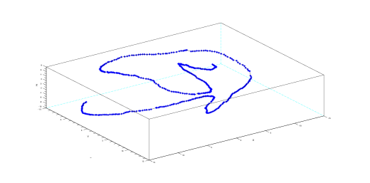
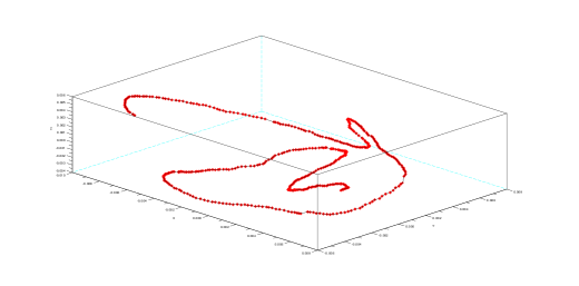
The results of applying dimensionality reduction using stochastic PCA and diffusion maps for the first videoclip are shown in Figure 3.

(a) Stochastic PCA

(b) Diffusion maps

Figure 3: Projection of each frame of the first videoclip ($15\min$) in $\mathbbm{R}^{3}$ using 3(a) one instance of stochastic PCA and 3(b) diffusion map at scale $t=2$.

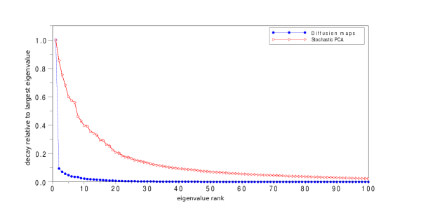
From Figure 3 it is not possible to be conclusive about which technique has better potential as part of the proposed modeling pipeline. To further investigage this, we compare the decay of the eigenvalues used in the diffusion map with that of the eigenvalues used in the stochastic PCA, relative to the largest eigenvalues. The diffusion map eigenvalues present a much shaper decay than the eigenvalues used in the stochastic PCA, Figure 4. This indicates that diffusion maps can represent the observed flow with fewer parameters.

Figure 4: The decay of the first $100$ eigenvalues used in the diffusion map compared to that of the eigenvalues used in the stochastic PCA, relative to the largest eigenvalues, for the first videoclip.

5 Conclusion and Future work

The image-based fluid modeling approach proposed in this work is part of a larger effort with applications to the online monitoring of ocean conditions for aiding offshore processes of oil drilling, among others.

With dimensionality reduction it is possible to represent the original data with a data-driven model with a small number of parameters. Using diffusion maps, these parameters reveal intrinsic structure of the original data, keeping the most relevant observable characteristics, while our experiments show that PCA was not as efficient in this sense. Building on such reduced model we proposed the main ideas of a stochastic model to account for remaining factors.

Work is underway to produce techniques for detailed machine learning and inference based on this model. The final complete model should be able to capture the patterns of fluid surface motion in a way that, when statistically sampling from this model, we should obtain a sequence of images that can reproduce the observed fluid behavior through time. In the future this can then be used to help infer the state of the ocean surface in a new video sequence. We have also been considering the use of video streams from multiple views to improve quality and robustness.

References

- de la Porte et al., (2008) de la Porte, J., Herbst, B. M. Hereman, H. & van der Walt, S. J. An Introduction to Diffusion Maps. Proceedings of the 19th Symposium of the Pattern Recognition Association of South Africa; 26-28 de novembro de 2008; Prasa. Cape Town: F. Nicolls, University of Cape Town, South Africa, 2008. pp. 15-25.
- Golub & Van Loan, (1996) Golub, G. H. & Van Loan, C. F. Matrix computations. 3 ed. Baltimore : Johns Hopkins University Press, 1996.
- Halko et al., (2010) Halko, N.; Martinsson, P. G.; Shkolnisky, Y. & Tygert, M. An algorithm for the principal component analysis of large data sets. SIAM Journal on Scientific Computing, vol. 33, n. 5, pp. 2580-2594, 2011.
- Halko et al., (2011) Halko, N.; Martinsson, P. G. & Tropp, J. A. Finding structure with randomness: Probabilistic algorithms for constructing approximate matrix decompositions. SIAM Review, vol. 53, n. 2, pp. 217-288, 2011.
- Hastie & et al., (2013) Hastie, T.; Tibshirani, R. & Friedman, J. The elements of statistical learning: Data mining, inference, and prediction. Springer, 2013.
- Jolliffe, (2002) Jolliffe, I. T. Principal component analysis. 2 ed. New York : Springer, 2002.
- Lafon & Lee, (2006) Lafon, S. & Lee, A. Diffusion maps and coarse-graining: A unified framework for dimensionality reduction, graph partitioning, and data set parameterization. Pattern Analysis and Machine Intelligence, IEEE Transactions on, vol. 28, n. 9, pp. 1393-1403, 2006.
- Mumford & Desolneux, (2010) Mumford, D. & Desolneux, A. Pattern theory: the stochastic analysis of real-world signal. CRC Press, 2010.