Strongly Intensive Measures for
Transverse Momentum and Particle Number Fluctuations

Mark I. Gorenstein Bogolyubov Institute for Theoretical Physics, Kiev, Ukraine Frankfurt Institute for Advanced Studies, Frankfurt, Germany    Katarzyna Grebieszkow Faculty of Physics, Warsaw University of Technology, Warsaw, Poland
Abstract

Strongly intensive measures Δ[PT,N]Δsubscript𝑃𝑇𝑁\Delta[P_{T},N] and Σ[PT,N]Σsubscript𝑃𝑇𝑁\Sigma[P_{T},N] are used to study the event-by-event fluctuations of the transverse momentum PTsubscript𝑃𝑇P_{T} and particle multiplicity N𝑁N in nucleus-nucleus collisions. A special normalization for these fluctuation measures ensures that they are dimensionless and yields a common scale required for a quantitative comparison of fluctuations. In this paper basic properties of the Δ[PT,N]Δsubscript𝑃𝑇𝑁\Delta[P_{T},N] and Σ[PT,N]Σsubscript𝑃𝑇𝑁\Sigma[P_{T},N] measures are tested within different phenomenological models using the Monte Carlo simulations (the so-called fast generators) and analytical solutions. The obtained results are helpful to elucidate the properties of the Δ[PT,N]Δsubscript𝑃𝑇𝑁\Delta[P_{T},N] and Σ[PT,N]Σsubscript𝑃𝑇𝑁\Sigma[P_{T},N] measures.

pacs:
12.40.-y, 12.40.Ee

I Introduction

The main motivation for the experiments studies on relativistic nucleus-nucleus (A+A) collisions is to create and study strongly interacting matter. Experimental and theoretical investigations of event-by-event (e-by-e) fluctuations in A+A collisions produce new information about its properties. E-by-e fluctuations can be also an important tool for localizing the phase boundary and the critical point of the QCD matter. In particular, significant increase of transverse momentum and multiplicity fluctuations are expected in a vicinity of the critical point crit . One can probe different regions of the phase diagram by varying the collision energy and the size of colliding nuclei size . A possibility to observe signatures of the critical point inspired the energy and system size scan program of the NA61/SHINE Collaboration at the CERN Super Proton Synchrotron (SPS) Ga:2009 and the low energy scan program of the STAR and PHENIX Collaborations at the Brookhaven National Laboratory’s Relativistic Heavy Ion Collider (BNL RHIC) RHIC-SCAN . In these studies one measures and then compares the e-by-e fluctuations in collisions of different nuclei at different collision energies. The average sizes of created physical systems and their e-by-e fluctuations are expected to be rather different KGBG:2010 . This strongly affects the observed hadron fluctuations, and consequently the measured quantities do not describe local physical properties of the system but rather reflect the system size fluctuations. For instance, A+A collisions with different centralities may produce a system with approximately the same local properties (e.g., the same temperature and baryonic chemical potential) but with the volume changing significantly from interaction to interaction. Note that in high energy collisions the average volume of created matter and its variations from collision to collision are usually out of experimental control, i.e. the volume variations are difficult or even impossible to measure. Therefore, a suitable choice of statistical tools for the study of e-by-e fluctuations is really important.

In statistical mechanics, an extensive quantity is proportional to the system volume V𝑉V, whereas an intensive one has fixed finite value in the thermodynamical limit V𝑉V\rightarrow\infty. Intensive quantities are used to describe local properties of a physical system. In particular, the equation of state of the matter is usually formulated in terms of intensive physical quantities, e.g., the pressure is considered as a function of temperature and chemical potentials.

The strongly intensive quantities have been introduced in Ref. GG:2011 . Within the grand canonical ensemble formulation of statistical mechanics they are independent of the average volume and volume fluctuations. Similar properties take place in the model of independent sources: the strongly intensive measures of fluctuations are independent of the average number of sources and of fluctuations of the number of sources. The strongly intensive measures Δ[A,B]Δ𝐴𝐵\Delta[A,B] and Σ[A,B]Σ𝐴𝐵\Sigma[A,B] are suggested for studies of e-by-e fluctuations of hadron production in heavy ion collisions at high energies. They are defined using two arbitrary extensive quantities A𝐴A and B𝐵B. In the present paper we consider a pair of extensive variables: the transverse momentum A=PT=pT(1)+pT(N)𝐴subscript𝑃𝑇superscriptsubscript𝑝𝑇1superscriptsubscript𝑝𝑇𝑁A=P_{T}=p_{T}^{(1)}+\dots p_{T}^{(N)}, where pT(i)subscriptsuperscript𝑝𝑖𝑇p^{(i)}_{T} is the absolute value of the ithsuperscript𝑖thi^{{\rm th}} particle transverse momentum, and the number of particles B=N𝐵𝑁B=N. The measures Δ[PT,N]Δsubscript𝑃𝑇𝑁\Delta[P_{T},N] and Σ[PT,N]Σsubscript𝑃𝑇𝑁\Sigma[P_{T},N] were studied recently within the ultra-relativistic quantum molecular dynamics (UrQMD) simulations in Ref. KG:APP2012 . The measures Δ[A,B]Δ𝐴𝐵\Delta[A,B] and Σ[A,B]Σ𝐴𝐵\Sigma[A,B] in the case of two hadron multiplicities A𝐴A and B𝐵B were considered within the hadron-string dynamics (HSD) transport model in Ref. HSD . To simplify notations we sometimes use X=PT𝑋subscript𝑃𝑇X=P_{T} and xi=pT(i)subscript𝑥𝑖superscriptsubscript𝑝𝑇𝑖x_{i}=p_{T}^{(i)}. Note that our consideration is valid also for other motional variables X𝑋X, e.g., the system energy X=E=ϵ1++ϵN𝑋𝐸subscriptitalic-ϵ1subscriptitalic-ϵ𝑁X=E=\epsilon_{1}+\dots+\epsilon_{N}. The strongly intensive measure Δ[X,N]Δ𝑋𝑁\Delta[X,N] and Σ[X,N]Σ𝑋𝑁\Sigma[X,N] are defined as GG:2011 :

Δ[X,N]=1CΔ[Nω[X]Xω[N]],Δ𝑋𝑁1subscript𝐶Δdelimited-[]delimited-⟨⟩𝑁𝜔delimited-[]𝑋delimited-⟨⟩𝑋𝜔delimited-[]𝑁\displaystyle\Delta[X,N]\leavevmode\nobreak\ =\leavevmode\nobreak\ \frac{1}{C_{\Delta}}\Big{[}\langle N\rangle\,\omega[X]\leavevmode\nobreak\ -\leavevmode\nobreak\ \langle X\rangle\,\omega[N]\Big{]}\leavevmode\nobreak\ , (1)
Σ[X,N]=1CΣ[Nω[X]+Xω[N] 2(XNXN)],Σ𝑋𝑁1subscript𝐶Σdelimited-[]delimited-⟨⟩𝑁𝜔delimited-[]𝑋delimited-⟨⟩𝑋𝜔delimited-[]𝑁2delimited-⟨⟩𝑋𝑁delimited-⟨⟩𝑋delimited-⟨⟩𝑁\displaystyle\Sigma[X,N]\leavevmode\nobreak\ =\leavevmode\nobreak\ \frac{1}{C_{\Sigma}}\Big{[}\langle N\rangle\,\omega[X]\leavevmode\nobreak\ +\leavevmode\nobreak\ \langle X\rangle\,\omega[N]\leavevmode\nobreak\ -\leavevmode\nobreak\ 2\Big{(}\langle X\,N\rangle\leavevmode\nobreak\ -\leavevmode\nobreak\ \langle X\rangle\langle N\rangle\Big{)}\Big{]}\leavevmode\nobreak\ , (2)

where

ω[X]=X2X2X,ω[N]=N2N2Nformulae-sequence𝜔delimited-[]𝑋delimited-⟨⟩superscript𝑋2superscriptdelimited-⟨⟩𝑋2delimited-⟨⟩𝑋𝜔delimited-[]𝑁delimited-⟨⟩superscript𝑁2superscriptdelimited-⟨⟩𝑁2delimited-⟨⟩𝑁\displaystyle\omega[X]\leavevmode\nobreak\ =\leavevmode\nobreak\ \frac{\langle X^{2}\rangle\leavevmode\nobreak\ -\leavevmode\nobreak\ \langle X\rangle^{2}}{\langle X\rangle}\leavevmode\nobreak\ ,\leavevmode\nobreak\ \leavevmode\nobreak\ \leavevmode\nobreak\ \leavevmode\nobreak\ \omega[N]\leavevmode\nobreak\ =\leavevmode\nobreak\ \frac{\langle N^{2}\rangle\leavevmode\nobreak\ -\leavevmode\nobreak\ \langle N\rangle^{2}}{\langle N\rangle}\leavevmode\nobreak\ (3)

are the scaled variances for X𝑋X and N𝑁N fluctuations, and CΔsubscript𝐶ΔC_{\Delta} and CΣsubscript𝐶ΣC_{\Sigma} are normalization factors. The notation delimited-⟨⟩\langle\dots\rangle represents the e-by-e averaging.

The first strongly intensive measure of fluctuations, the so-called ΦΦ\Phi measure, was introduced a long time ago in Ref. GM:1992 . There were many attempts to use the ΦΦ\Phi measure in the data analysis Phi_data ; d1 ; d2 ; d3 ; d4 ; d5 ; d6 and in theoretical models Phi_models ; m2 ; m3 ; m4 ; m5 ; m6 ; m7 ; m8a ; m8 ; m9 ; m10 ; m11 ; MRW:2004 ; m12 ; m13 ; m14 . In general, ΦΦ\Phi is a dimensional quantity and it does not assume a characteristic scale for a quantitative analysis of e-by-e fluctuations for different observables. Note that the latter properties were clearly disturbing.

In the recent paper GGP:2013 special normalization has been proposed for the ΔΔ\Delta and ΣΣ\Sigma fluctuation measures. It is used in the present study and ensures that measures (1) and (2) are dimensionless and yields a common scale required for a quantitative comparison of the e-by-e fluctuations. This normalization has been already used for the Δ[PT,N]Δsubscript𝑃𝑇𝑁\Delta[P_{T},N] and Σ[PT,N]Σsubscript𝑃𝑇𝑁\Sigma[P_{T},N] measures using the transport model of A+A collisions in Ref. GGP:2013 and for the ideal quantum gases within the grand canonical ensemble formulation GR:2013 . Note that the NA61 Collaboration has already started to use the strongly intensive measures to study e-by-e fluctuations in A+A collisions NA61-plan .

In the present paper several phenomenological models of hadron production are suggested and studied using the Monte Carlo (MC) simulations (the so-called fast generators). Analytical solutions for the proposed models are also presented and analyzed. These studies are helpful to elucidate properties of the Δ[PT,N]Δsubscript𝑃𝑇𝑁\Delta[P_{T},N] and Σ[PT,N]Σsubscript𝑃𝑇𝑁\Sigma[P_{T},N] measures. A search for possible signals for the phase transition and critical point in A+A collisions is outside of the scope of our paper. To achieve this goal one first needs to formulate suitable dynamical models for these phenomena.

The paper is organized as follows. In Sec. II we introduce two reference models. The first model is the independent particle model within which we calculate the normalization factors CΔsubscript𝐶ΔC_{\Delta} and CΣsubscript𝐶ΣC_{\Sigma} for Δ[X,N]Δ𝑋𝑁\Delta[X,N] and Σ[X,N]Σ𝑋𝑁\Sigma[X,N] quantities. The second model is the model of independent sources which is often used to analyze the data on nucleus-nucleus collisions. Section III presents examples of the MC simulations. Some of these examples correspond to different versions of the model of independent sources. Analytical solutions are also presented and analyzed. In Sec. IV the MC simulations and analytical consideration are used for the models where single particle momentum spectra are dependent on the number of the produced particles. In Sec. V results of statistical and transport models are presented. Using the UrQMD simulations we study effects of the centrality selection and limited detector acceptance and efficiency in A+A collisions. A summary in Sec. VI closes the article.

II Reference Models

In this section two simple models of particle production are presented. The first one is the independent particle model (IPM) which is used as a reference model to fix the normalization of the strongly intensive measures ΔΔ\Delta and ΣΣ\Sigma. Namely, properly normalized strongly intensive quantities assume the value one for the fluctuations given by the IPM. The second model is the model of independent sources. In this model, the values of ΔΔ\Delta and ΣΣ\Sigma for the system of sources are equal to their values for a single source.

II.1 Independent Particle Model

In Ref. GGP:2013 a special normalization for the strongly intensive measures Δ[A,B]Δ𝐴𝐵\Delta[A,B] and Σ[A,B]Σ𝐴𝐵\Sigma[A,B] has been proposed. In this subsection we present its derivation when A𝐴A is an extensive variable A=X𝐴𝑋A=X presented as a sum of single particle terms

X=x1+x2++xN,𝑋subscript𝑥1subscript𝑥2subscript𝑥𝑁\displaystyle X\leavevmode\nobreak\ =\leavevmode\nobreak\ x_{1}\leavevmode\nobreak\ +x_{2}\leavevmode\nobreak\ +\ldots\leavevmode\nobreak\ +x_{N}\leavevmode\nobreak\ , (4)

(e.g., the system energy E𝐸E or transverse momentum PTsubscript𝑃𝑇P_{T}) and B=N𝐵𝑁B=N is the number of particles. Inter-particle correlations are absent in the IPM, i.e. the probability of any multi-particle state is a product of probability distributions F(xj)𝐹subscript𝑥𝑗F(x_{j}) of single-particle variables xjsubscript𝑥𝑗x_{j}, and these probability distributions are the same for all j=1,,N𝑗1𝑁j=1,\ldots,N and independent of the number of particles N𝑁N :

FN(x1,x2,,xN)=𝒫(N)×F(x1)F(x2)××F(xN),subscript𝐹𝑁subscript𝑥1subscript𝑥2subscript𝑥𝑁𝒫𝑁𝐹subscript𝑥1𝐹subscript𝑥2𝐹subscript𝑥𝑁\displaystyle F_{N}(x_{1},x_{2},\dots,x_{N})\leavevmode\nobreak\ =\leavevmode\nobreak\ {\cal P}(N)\times F(x_{1})\,F(x_{2})\times\cdots\times F(x_{N})\leavevmode\nobreak\ , (5)

where 𝒫(N)𝒫𝑁{\cal P}(N) is an arbitrary multiplicity distribution of particles. The functions entering Eq. (5) satisfy the normalization conditions:

N𝒫(N)= 1,𝑑xF(x)= 1.formulae-sequencesubscript𝑁𝒫𝑁1differential-d𝑥𝐹𝑥1\displaystyle\sum_{N}{\cal P}(N)\leavevmode\nobreak\ =\leavevmode\nobreak\ 1\leavevmode\nobreak\ ,\leavevmode\nobreak\ \leavevmode\nobreak\ \leavevmode\nobreak\ \leavevmode\nobreak\ \leavevmode\nobreak\ \int dx\leavevmode\nobreak\ F(x)\leavevmode\nobreak\ =\leavevmode\nobreak\ 1\leavevmode\nobreak\ . (6)

The averaging procedure for kthsuperscript𝑘thk^{{\rm th}} moments of any multiparticle observable A𝐴A reads:

Ak=N𝒫(N)𝑑x1𝑑x2𝑑xNF(x1)F(x2)××F(xN)[A(x1,x2,,xN)]k.delimited-⟨⟩superscript𝐴𝑘subscript𝑁𝒫𝑁differential-dsubscript𝑥1differential-dsubscript𝑥2differential-dsubscript𝑥𝑁𝐹subscript𝑥1𝐹subscript𝑥2𝐹subscript𝑥𝑁superscriptdelimited-[]𝐴subscript𝑥1subscript𝑥2subscript𝑥𝑁𝑘\displaystyle\langle A^{k}\rangle\leavevmode\nobreak\ =\leavevmode\nobreak\ \sum_{N}{\cal P}(N)\int dx_{1}dx_{2}\ldots dx_{N}F(x_{1})\,F(x_{2})\times\cdots\times F(x_{N})\leavevmode\nobreak\ \Big{[}A(x_{1},x_{2},\ldots,x_{N})\Big{]}^{k}\leavevmode\nobreak\ . (7)

For the first and second moments of X𝑋X and N𝑁N one obtains:

X=x¯N,X2=x2¯N+x¯2[N2N],XN=x¯N2,formulae-sequencedelimited-⟨⟩𝑋¯𝑥delimited-⟨⟩𝑁formulae-sequencedelimited-⟨⟩superscript𝑋2¯superscript𝑥2delimited-⟨⟩𝑁superscript¯𝑥2delimited-[]delimited-⟨⟩superscript𝑁2delimited-⟨⟩𝑁delimited-⟨⟩𝑋𝑁¯𝑥delimited-⟨⟩superscript𝑁2\displaystyle\langle X\rangle=\overline{x}\cdot\langle N\rangle\leavevmode\nobreak\ ,\leavevmode\nobreak\ \leavevmode\nobreak\ \leavevmode\nobreak\ \leavevmode\nobreak\ \langle X^{2}\rangle=\overline{x^{2}}\cdot\langle N\rangle+\overline{x}^{2}\cdot\left[\langle N^{2}\rangle-\langle N\rangle\right]\leavevmode\nobreak\ ,\leavevmode\nobreak\ \leavevmode\nobreak\ \leavevmode\nobreak\ \leavevmode\nobreak\ \langle XN\rangle=\overline{x}\cdot\langle N^{2}\rangle\leavevmode\nobreak\ , (8)

where

Nk=N𝒫(N)Nk,xk¯=𝑑xF(x)xk.formulae-sequencedelimited-⟨⟩superscript𝑁𝑘subscript𝑁𝒫𝑁superscript𝑁𝑘¯superscript𝑥𝑘differential-d𝑥𝐹𝑥superscript𝑥𝑘\displaystyle\langle N^{k}\rangle\leavevmode\nobreak\ =\leavevmode\nobreak\ \sum_{N}{\cal P}(N)\,N^{k}\leavevmode\nobreak\ ,\leavevmode\nobreak\ \leavevmode\nobreak\ \leavevmode\nobreak\ \leavevmode\nobreak\ \leavevmode\nobreak\ \overline{x^{k}}\leavevmode\nobreak\ =\leavevmode\nobreak\ \int dx\,F(x)\,x^{k}\leavevmode\nobreak\ . (9)

Note that the overline denotes averaging over single particle inclusive distribution, whereas delimited-⟨⟩\langle\dots\rangle represents event averaging over multiparticle states of the system, e.g., e-by-e averaging over hadrons detected in A+A collisions.

Using Eq. (8), one finds

ω[X]X2X2X=x2¯x¯2x¯+x¯N2N2Nω[x]+x¯ω[N],𝜔delimited-[]𝑋delimited-⟨⟩superscript𝑋2delimited-⟨⟩superscript𝑋2delimited-⟨⟩𝑋¯superscript𝑥2superscript¯𝑥2¯𝑥¯𝑥delimited-⟨⟩superscript𝑁2superscriptdelimited-⟨⟩𝑁2delimited-⟨⟩𝑁𝜔delimited-[]𝑥¯𝑥𝜔delimited-[]𝑁\displaystyle\omega[X]\equiv\leavevmode\nobreak\ \frac{\langle X^{2}\rangle-\langle X^{2}\rangle}{\langle X\rangle}\leavevmode\nobreak\ =\leavevmode\nobreak\ \frac{\overline{x^{2}}-\overline{x}^{2}}{\overline{x}}\leavevmode\nobreak\ +\leavevmode\nobreak\ \overline{x}\cdot\frac{\langle N^{2}\rangle-\langle N\rangle^{2}}{\langle N\rangle}\leavevmode\nobreak\ \equiv\leavevmode\nobreak\ \omega[x]\leavevmode\nobreak\ +\leavevmode\nobreak\ \overline{x}\cdot\omega[N]\leavevmode\nobreak\ , (10)
XNXN=x¯[N2N2]x¯Nω[N],delimited-⟨⟩𝑋𝑁delimited-⟨⟩𝑋delimited-⟨⟩𝑁¯𝑥delimited-[]delimited-⟨⟩superscript𝑁2superscriptdelimited-⟨⟩𝑁2¯𝑥delimited-⟨⟩𝑁𝜔delimited-[]𝑁\displaystyle\langle XN\rangle\leavevmode\nobreak\ -\leavevmode\nobreak\ \langle X\rangle\,\langle N\rangle\leavevmode\nobreak\ =\leavevmode\nobreak\ \overline{x}\cdot\Big{[}\langle N^{2}\rangle\leavevmode\nobreak\ -\leavevmode\nobreak\ \langle N\rangle^{2}\Big{]}\leavevmode\nobreak\ \equiv\leavevmode\nobreak\ \overline{x}\cdot\langle N\rangle\leavevmode\nobreak\ \omega[N]\leavevmode\nobreak\ , (11)

and finally,

Δ[X,N]=1CΔ[Nω[X]Xω[N]]=ω[x]NCΔ,Δ𝑋𝑁1subscript𝐶Δdelimited-[]delimited-⟨⟩𝑁𝜔delimited-[]𝑋delimited-⟨⟩𝑋𝜔delimited-[]𝑁𝜔delimited-[]𝑥delimited-⟨⟩𝑁subscript𝐶Δ\displaystyle\Delta[X,N]\leavevmode\nobreak\ =\leavevmode\nobreak\ \frac{1}{C_{\Delta}}\leavevmode\nobreak\ \Big{[}\langle N\rangle\,\omega[X]\leavevmode\nobreak\ -\leavevmode\nobreak\ \langle X\rangle\,\omega[N]\Big{]}\leavevmode\nobreak\ =\leavevmode\nobreak\ \frac{\omega[x]\cdot\langle N\rangle}{C_{\Delta}}\leavevmode\nobreak\ , (12)
Σ[X,N]=1CΣ[Nω[X]+Xω[N] 2(XNXN)]=ω[x]NCΣ.Σ𝑋𝑁1subscript𝐶Σdelimited-[]delimited-⟨⟩𝑁𝜔delimited-[]𝑋delimited-⟨⟩𝑋𝜔delimited-[]𝑁2delimited-⟨⟩𝑋𝑁delimited-⟨⟩𝑋delimited-⟨⟩𝑁𝜔delimited-[]𝑥delimited-⟨⟩𝑁subscript𝐶Σ\displaystyle\Sigma[X,N]\leavevmode\nobreak\ =\leavevmode\nobreak\ \frac{1}{C_{\Sigma}}\leavevmode\nobreak\ \Big{[}\langle N\rangle\,\omega[X]\leavevmode\nobreak\ +\leavevmode\nobreak\ \langle X\rangle\,\omega[N]\leavevmode\nobreak\ -\leavevmode\nobreak\ 2\Big{(}\langle X\,N\rangle\leavevmode\nobreak\ -\leavevmode\nobreak\ \langle X\rangle\langle N\rangle\Big{)}\Big{]}\leavevmode\nobreak\ =\leavevmode\nobreak\ \frac{\omega[x]\cdot\langle N\rangle}{C_{\Sigma}}\leavevmode\nobreak\ . (13)

The requirement that

Δ[X,N]=Σ[X,N]= 1Δ𝑋𝑁Σ𝑋𝑁1\displaystyle\Delta[X,N]\leavevmode\nobreak\ =\leavevmode\nobreak\ \Sigma[X,N]\leavevmode\nobreak\ =\leavevmode\nobreak\ 1 (14)

for the IPM leads thus to the normalization factors

CΔ=CΣ=ω[x]N,ω[x]x2¯x¯2x¯.formulae-sequencesubscript𝐶Δsubscript𝐶Σ𝜔delimited-[]𝑥delimited-⟨⟩𝑁𝜔delimited-[]𝑥¯superscript𝑥2superscript¯𝑥2¯𝑥\displaystyle C_{\Delta}\leavevmode\nobreak\ =\leavevmode\nobreak\ C_{\Sigma}=\leavevmode\nobreak\ \omega[x]\cdot\langle N\rangle\leavevmode\nobreak\ ,\leavevmode\nobreak\ \leavevmode\nobreak\ \leavevmode\nobreak\ \leavevmode\nobreak\ \leavevmode\nobreak\ \omega[x]\leavevmode\nobreak\ \equiv\leavevmode\nobreak\ \frac{\overline{x^{2}}\leavevmode\nobreak\ -\leavevmode\nobreak\ \overline{x}^{2}}{\overline{x}}\leavevmode\nobreak\ . (15)

The normalization factors (15) are suggested to be used both in theoretical models and for the data analysis (see Ref. GGP:2013 for further details of the normalization procedure).

According to the current classification the ΦΦ\Phi measure GM:1992 belongs to the ΣΣ\Sigma family GG:2011 . It can be calculated as

ΦX=[x¯ω[x]]1/2[Σ[X,N] 1].subscriptΦ𝑋superscriptdelimited-[]¯𝑥𝜔delimited-[]𝑥12delimited-[]Σ𝑋𝑁1\displaystyle\Phi_{X}\leavevmode\nobreak\ =\leavevmode\nobreak\ \Big{[}\overline{x}\,\omega[x]\Big{]}^{1/2}\,\Big{[}\sqrt{\Sigma[X,N]}\leavevmode\nobreak\ -\leavevmode\nobreak\ 1\Big{]}\leavevmode\nobreak\ . (16)

The representation of X𝑋X with Eq. (4) as the sum of single particle variables xisubscript𝑥𝑖x_{i} is an evident feature of the IPM. Thus, one needs such a representation to calculate the normalization factors CΔsubscript𝐶ΔC_{\Delta} and CΣsubscript𝐶ΣC_{\Sigma}. Such a representation of the extensive motional variable is, however, not necessarily needed for the e-by-e measurements. For example, the system energy E𝐸E (or transverse momentum PTsubscript𝑃𝑇P_{T}) can be measured by a calorimeter without determining individual single particle contributions.

It was proven GGP:2013 that the IPM relation (14) is valid also in two models. The first model is statistical mechanics for the Boltzmann ideal gas within the grand canonical ensemble. The second model is the mixed event procedure which creates a sample of artificial events, where each particle is taken from different physical events. These model constructions play an important role as reference model. The deviations of real data from the IPM results (14) can be used to clarify the physical properties of the system. It resembles the situation with particle number distributions. One prefers to use the Poisson distribution P(N)=exp(N¯)N¯N/N!𝑃𝑁¯𝑁superscript¯𝑁𝑁𝑁P(N)=\exp\left(-\,\overline{N}\right)\,\overline{N}^{N}/{N!}  with ω[N]=1𝜔delimited-[]𝑁1\omega[N]=1 as a reference model. Another reference value ω[N]=0𝜔delimited-[]𝑁0\omega[N]=0 corresponds to N=const𝑁constN={\rm const}, where the N𝑁N-fluctuations are absent. The fluctuations for any particle number distribution 𝒫(N)𝒫𝑁{\cal P}(N) is then clarified by the comparison of the calculated (or measured) scaled variance ω[N]𝜔delimited-[]𝑁\omega[N] with its reference value of ω[N]=1𝜔delimited-[]𝑁1\omega[N]=1. The relation ω[N]>1𝜔delimited-[]𝑁1\omega[N]>1 (or ω[N]1much-greater-than𝜔delimited-[]𝑁1\omega[N]\gg 1) corresponds to “large” (or “very large”) fluctuations of N𝑁N, and ω[N]<1𝜔delimited-[]𝑁1\omega[N]<1 (or ω[N]1much-less-than𝜔delimited-[]𝑁1\omega[N]\ll 1) to “small” (or “very small”) fluctuations.

II.2 Model of Independent Sources

In this subsection we consider a model of independent sources (MIS) for multi-particle production. In this model the number of sources, NSsubscript𝑁𝑆N_{S}, changes from event to event. The sources are statistically identical and independent of each other. A famous example of the MIS is the wounded nucleon model WNM for A+A collisions . Two fluctuating extensive quantities X𝑋X and N𝑁N can be expressed as

X=X1+X2++XNS,N=n1+n2++nNS,formulae-sequence𝑋subscript𝑋1subscript𝑋2subscript𝑋subscript𝑁𝑆𝑁subscript𝑛1subscript𝑛2subscript𝑛subscript𝑁𝑆\displaystyle X\leavevmode\nobreak\ =\leavevmode\nobreak\ X_{1}\leavevmode\nobreak\ +X_{2}\leavevmode\nobreak\ +\ldots\leavevmode\nobreak\ +X_{N_{S}}\leavevmode\nobreak\ ,\leavevmode\nobreak\ \leavevmode\nobreak\ \leavevmode\nobreak\ \leavevmode\nobreak\ \leavevmode\nobreak\ N\leavevmode\nobreak\ =\leavevmode\nobreak\ n_{1}\leavevmode\nobreak\ +n_{2}\leavevmode\nobreak\ +\ldots\leavevmode\nobreak\ +n_{N_{S}}\leavevmode\nobreak\ , (17)

where njsubscript𝑛𝑗n_{j} denotes the number of particles emitted from the jthsuperscript𝑗thj^{{\rm th}} source (j=1,,NS𝑗1subscript𝑁𝑆j=1,\ldots,N_{S}), and Xj=x1++xnjsubscript𝑋𝑗subscript𝑥1subscript𝑥subscript𝑛𝑗X_{j}=x_{1}+\dots+x_{n_{j}} is the contribution from the jthsuperscript𝑗thj^{{\rm th}} source to the quantity X𝑋X.

Overline notations will be used for the averages connected to a single source. The single-source quantities are independent of NSsubscript𝑁𝑆N_{S} and have the properties of intensive quantities. The single-source distribution FS(XS,n)subscript𝐹𝑆subscript𝑋𝑆𝑛F_{S}(X_{S},n) is assumed to be statistically identical for all sources, thus, for all j=1,,NS𝑗1subscript𝑁𝑆j=1,\dots,N_{S} it follows:

Xjk¯XSk¯,njk¯nk¯,Xjnj¯XSn¯,formulae-sequence¯superscriptsubscript𝑋𝑗𝑘¯superscriptsubscript𝑋𝑆𝑘formulae-sequence¯superscriptsubscript𝑛𝑗𝑘¯superscript𝑛𝑘¯subscript𝑋𝑗subscript𝑛𝑗¯subscript𝑋𝑆𝑛\displaystyle\overline{X_{j}^{k}}\leavevmode\nobreak\ \equiv\leavevmode\nobreak\ \overline{X_{S}^{k}}\leavevmode\nobreak\ ,\leavevmode\nobreak\ \leavevmode\nobreak\ \leavevmode\nobreak\ \leavevmode\nobreak\ \overline{n_{j}^{k}}\leavevmode\nobreak\ \equiv\leavevmode\nobreak\ \overline{n^{k}}\leavevmode\nobreak\ ,\leavevmode\nobreak\ \leavevmode\nobreak\ \leavevmode\nobreak\ \overline{X_{j}n_{j}}\leavevmode\nobreak\ \equiv\leavevmode\nobreak\ \overline{X_{S}n}\leavevmode\nobreak\ , (18)

where XSk¯¯superscriptsubscript𝑋𝑆𝑘\overline{X_{S}^{k}}, nk¯¯superscript𝑛𝑘\overline{n^{k}}, and XSn¯¯subscript𝑋𝑆𝑛\overline{X_{S}\,n} (for k=1,2𝑘12k=1,2) are the first and second moments of the distribution FS(XS,n)subscript𝐹𝑆subscript𝑋𝑆𝑛F_{S}(X_{S},n) for a single source. The sources are assumed to be independent. This gives at ij𝑖𝑗i\neq j:

XiXj¯XS¯2,ninj¯n¯2,Xinj¯XS¯n¯.formulae-sequence¯subscript𝑋𝑖subscript𝑋𝑗superscript¯subscript𝑋𝑆2formulae-sequence¯subscript𝑛𝑖subscript𝑛𝑗superscript¯𝑛2¯subscript𝑋𝑖subscript𝑛𝑗¯subscript𝑋𝑆¯𝑛\displaystyle\overline{X_{i}X_{j}}\leavevmode\nobreak\ \equiv\leavevmode\nobreak\ \overline{X_{S}}^{2}\leavevmode\nobreak\ ,\leavevmode\nobreak\ \leavevmode\nobreak\ \leavevmode\nobreak\ \leavevmode\nobreak\ \overline{n_{i}n_{j}}\leavevmode\nobreak\ \equiv\leavevmode\nobreak\ \overline{n}^{2}\leavevmode\nobreak\ ,\leavevmode\nobreak\ \leavevmode\nobreak\ \leavevmode\nobreak\ \overline{X_{i}n_{j}}\leavevmode\nobreak\ \equiv\leavevmode\nobreak\ \overline{X_{S}}\leavevmode\nobreak\ \overline{n}\leavevmode\nobreak\ . (19)

Using Eqs. (18) and (19) one finds for the event averages:

X=XS¯NS,X2=XS2¯NS+XS¯2[NS2NS],formulae-sequencedelimited-⟨⟩𝑋¯subscript𝑋𝑆delimited-⟨⟩subscript𝑁𝑆delimited-⟨⟩superscript𝑋2¯superscriptsubscript𝑋𝑆2delimited-⟨⟩subscript𝑁𝑆superscript¯subscript𝑋𝑆2delimited-[]delimited-⟨⟩superscriptsubscript𝑁𝑆2delimited-⟨⟩subscript𝑁𝑆\displaystyle\langle X\rangle\leavevmode\nobreak\ =\leavevmode\nobreak\ \overline{X_{S}}\cdot\langle N_{S}\rangle\leavevmode\nobreak\ ,\leavevmode\nobreak\ \leavevmode\nobreak\ \leavevmode\nobreak\ \leavevmode\nobreak\ \langle X^{2}\rangle\leavevmode\nobreak\ =\leavevmode\nobreak\ \overline{X_{S}^{2}}\cdot\langle N_{S}\rangle\leavevmode\nobreak\ +\leavevmode\nobreak\ \overline{X_{S}}^{2}\leavevmode\nobreak\ \left[\langle N_{S}^{2}\rangle\leavevmode\nobreak\ -\leavevmode\nobreak\ \langle N_{S}\rangle\right]\leavevmode\nobreak\ , (20)
N=n¯NS,N2=n2¯NS+n¯2[NS2NS],formulae-sequencedelimited-⟨⟩𝑁¯𝑛delimited-⟨⟩subscript𝑁𝑆delimited-⟨⟩superscript𝑁2¯superscript𝑛2delimited-⟨⟩subscript𝑁𝑆superscript¯𝑛2delimited-[]delimited-⟨⟩superscriptsubscript𝑁𝑆2delimited-⟨⟩subscript𝑁𝑆\displaystyle\langle N\rangle\leavevmode\nobreak\ =\leavevmode\nobreak\ \overline{n}\leavevmode\nobreak\ \langle N_{S}\rangle\leavevmode\nobreak\ ,\leavevmode\nobreak\ \leavevmode\nobreak\ \leavevmode\nobreak\ \leavevmode\nobreak\ \langle N^{2}\rangle\leavevmode\nobreak\ =\leavevmode\nobreak\ \overline{n^{2}}\cdot\langle N_{S}\rangle\leavevmode\nobreak\ +\leavevmode\nobreak\ \overline{n}^{2}\cdot\left[\langle N_{S}^{2}\rangle\leavevmode\nobreak\ -\leavevmode\nobreak\ \langle N_{S}\rangle\right]\leavevmode\nobreak\ , (21)
XN=XSn¯NS+XS¯n¯[NS2NS].delimited-⟨⟩𝑋𝑁¯subscript𝑋𝑆𝑛delimited-⟨⟩subscript𝑁𝑆¯subscript𝑋𝑆¯𝑛delimited-[]delimited-⟨⟩superscriptsubscript𝑁𝑆2delimited-⟨⟩subscript𝑁𝑆\displaystyle\langle X\,N\rangle\leavevmode\nobreak\ =\leavevmode\nobreak\ \overline{X_{S}\,n}\leavevmode\nobreak\ \langle N_{S}\rangle\leavevmode\nobreak\ +\leavevmode\nobreak\ \overline{X_{S}}\leavevmode\nobreak\ \overline{n}\cdot\left[\langle N_{S}^{2}\rangle\leavevmode\nobreak\ -\leavevmode\nobreak\ \langle N_{S}\rangle\right]\leavevmode\nobreak\ . (22)

A probability distribution 𝒫S(NS)subscript𝒫𝑆subscript𝑁𝑆{\cal P}_{S}(N_{S}) of the number of sources is needed to calculate NSdelimited-⟨⟩subscript𝑁𝑆\langle N_{S}\rangle and NS2delimited-⟨⟩superscriptsubscript𝑁𝑆2\langle N_{S}^{2}\rangle and, in general, it is unknown.

Using Eqs. (20-22) one obtains:

ω[X]𝜔delimited-[]𝑋\displaystyle\omega[X] X2X2X=XS2¯XS¯2XS¯+XS¯NS2NS2NSω[XS]+XS¯ω[NS],absentdelimited-⟨⟩superscript𝑋2superscriptdelimited-⟨⟩𝑋2delimited-⟨⟩𝑋¯superscriptsubscript𝑋𝑆2superscript¯subscript𝑋𝑆2¯subscript𝑋𝑆¯subscript𝑋𝑆delimited-⟨⟩superscriptsubscript𝑁𝑆2superscriptdelimited-⟨⟩subscript𝑁𝑆2delimited-⟨⟩subscript𝑁𝑆𝜔delimited-[]subscript𝑋𝑆¯subscript𝑋𝑆𝜔delimited-[]subscript𝑁𝑆\displaystyle\equiv\leavevmode\nobreak\ \frac{\langle X^{2}\rangle-\langle X\rangle^{2}}{\langle X\rangle}=\frac{\overline{X_{S}^{2}}-\overline{X_{S}}^{2}}{\overline{X_{S}}}+\overline{X_{S}}\cdot\frac{\langle N_{S}^{2}\rangle-\langle N_{S}\rangle^{2}}{\langle N_{S}\rangle}\leavevmode\nobreak\ \equiv\leavevmode\nobreak\ \omega[X_{S}]\leavevmode\nobreak\ +\leavevmode\nobreak\ \overline{X_{S}}\cdot\omega[N_{S}]\leavevmode\nobreak\ , (23)
ω[N]𝜔delimited-[]𝑁\displaystyle\omega[N] N2N2N=n2¯n¯2n¯+n¯NS2NS2NSω[n]+n¯ω[NS],absentdelimited-⟨⟩superscript𝑁2superscriptdelimited-⟨⟩𝑁2delimited-⟨⟩𝑁¯superscript𝑛2superscript¯𝑛2¯𝑛¯𝑛delimited-⟨⟩superscriptsubscript𝑁𝑆2superscriptdelimited-⟨⟩subscript𝑁𝑆2delimited-⟨⟩subscript𝑁𝑆𝜔delimited-[]𝑛¯𝑛𝜔delimited-[]subscript𝑁𝑆\displaystyle\equiv\leavevmode\nobreak\ \frac{\langle N^{2}\rangle\leavevmode\nobreak\ -\leavevmode\nobreak\ \langle N\rangle^{2}}{\langle N\rangle}\leavevmode\nobreak\ =\leavevmode\nobreak\ \frac{\overline{n^{2}}\leavevmode\nobreak\ -\leavevmode\nobreak\ \overline{n}^{2}}{\overline{n}}\leavevmode\nobreak\ +\leavevmode\nobreak\ \overline{n}\cdot\frac{\langle N_{S}^{2}\rangle\leavevmode\nobreak\ -\leavevmode\nobreak\ \langle N_{S}\rangle^{2}}{\langle N_{S}\rangle}\leavevmode\nobreak\ \equiv\leavevmode\nobreak\ \omega[n]\leavevmode\nobreak\ +\leavevmode\nobreak\ \overline{n}\cdot\omega[N_{S}]\leavevmode\nobreak\ , (24)

where ω[XS]𝜔delimited-[]subscript𝑋𝑆\omega[X_{S}] and ω[n]𝜔delimited-[]𝑛\omega[n] are the scaled variances for quantities XSsubscript𝑋𝑆X_{S} and n𝑛n referring to a single source. The scaled variances ω[X]𝜔delimited-[]𝑋\omega[X] and ω[N]𝜔delimited-[]𝑁\omega[N] are independent of the average number of sources NSdelimited-⟨⟩subscript𝑁𝑆\langle N_{S}\rangle. Thus, ω[X]𝜔delimited-[]𝑋\omega[X] and ω[N]𝜔delimited-[]𝑁\omega[N] are intensive quantities. However, they depend on the fluctuations of the number of sources via ω[NS]𝜔delimited-[]subscript𝑁𝑆\omega[N_{S}] and, therefore, they are not strongly intensive quantities.

From Eqs. (22-24) it follows:

Δ[X,N]Δ𝑋𝑁\displaystyle\Delta[X,N]\leavevmode\nobreak\ =1ω[x][ω[XS]x¯ω[n]].absent1𝜔delimited-[]𝑥delimited-[]𝜔delimited-[]subscript𝑋𝑆¯𝑥𝜔delimited-[]𝑛\displaystyle=\leavevmode\nobreak\ \frac{1}{\omega[x]}\leavevmode\nobreak\ \Big{[}\,\omega[X_{S}]\leavevmode\nobreak\ -\leavevmode\nobreak\ \overline{x}\cdot\omega[n]\,\Big{]}\leavevmode\nobreak\ . (25)
Σ[X,N]Σ𝑋𝑁\displaystyle\Sigma[X,N]\leavevmode\nobreak\ =1ω[x][ω[XS]+x¯ω[n] 2XSn¯x¯n¯2n¯],absent1𝜔delimited-[]𝑥delimited-[]𝜔delimited-[]subscript𝑋𝑆¯𝑥𝜔delimited-[]𝑛2¯subscript𝑋𝑆𝑛¯𝑥superscript¯𝑛2¯𝑛\displaystyle=\leavevmode\nobreak\ \frac{1}{\omega[x]}\leavevmode\nobreak\ \Big{[}\,\omega[X_{S}]\leavevmode\nobreak\ +\leavevmode\nobreak\ \overline{x}\cdot\omega[n]\leavevmode\nobreak\ -\leavevmode\nobreak\ 2\,\frac{\overline{X_{S}\,n}-\overline{x}\leavevmode\nobreak\ \overline{n}^{2}}{\overline{n}}\,\Big{]}\leavevmode\nobreak\ , (26)

where the relations x¯=XS¯/n¯=X/N¯𝑥¯subscript𝑋𝑆¯𝑛delimited-⟨⟩𝑋delimited-⟨⟩𝑁\overline{x}=\overline{X_{S}}/\overline{n}=\langle X\rangle/\langle N\rangle , and the normalization factors (15) have been used.

Note that the terms with NS2delimited-⟨⟩superscriptsubscript𝑁𝑆2\langle N_{S}^{2}\rangle, which are present in the expressions (20-22) for the second moments of X𝑋X and N𝑁N, are canceled out in the final expressions (25,26). From three second moments X2delimited-⟨⟩superscript𝑋2\langle X^{2}\rangle, N2delimited-⟨⟩superscript𝑁2\langle N^{2}\rangle, and XNdelimited-⟨⟩𝑋𝑁\langle X\,N\rangle only two linear combinations independent of NS2delimited-⟨⟩superscriptsubscript𝑁𝑆2\langle N_{S}^{2}\rangle can be constructed. They are defined as the strongly intensive quantities ΔΔ\Delta and ΣΣ\Sigma. To remove the dependence on NSdelimited-⟨⟩subscript𝑁𝑆\langle N_{S}\rangle, the strongly intensive quantities should be in a form of reducible fractions. This is achieved due to the normalization factors (15).

Only the first and second moments of X𝑋X and N𝑁N are required in order to define the strongly intensive quantities ΔΔ\Delta and ΣΣ\Sigma. However, in order to calculate the proposed normalization factors CΣsubscript𝐶ΣC_{\Sigma} and CΔsubscript𝐶ΔC_{\Delta}, additional information is needed, namely the second moment x2¯¯superscript𝑥2\overline{x^{2}} of single-particle distribution F(x)𝐹𝑥F(x). Note that the first moment x¯¯𝑥\overline{x} can be calculated as x¯=X/N¯𝑥delimited-⟨⟩𝑋delimited-⟨⟩𝑁\overline{x}=\langle X\rangle/\langle N\rangle, and thus to find it the single particle distribution F(x)𝐹𝑥F(x) is not necessarily needed.

The IPM and MIS have similar structure. The difference is that the number of sources NSsubscript𝑁𝑆N_{S} in the MIS is replaced by the number of particles N𝑁N in the IPM. Each source can produce many particles, and the number of these particles varies from source to source and from event to event. Besides, the physical quantity XSsubscript𝑋𝑆X_{S} for particles emitted from the same source may include inter-particle correlations. Therefore, in general, the MIS does not satisfy the assumptions of the IPM. Nevertheless, a formal similarity between the two models can be exploited and gives the following rule of one to one correspondence: all results for the IPM can be found from the expressions obtained within the MIS, assuming artificially that each source always produces exactly one particle. In this case one finds

n¯=1,ω[n]=0,ω[XS]=ω[x],XSn¯=x¯,formulae-sequence¯𝑛1formulae-sequence𝜔delimited-[]𝑛0formulae-sequence𝜔delimited-[]subscript𝑋𝑆𝜔delimited-[]𝑥¯subscript𝑋𝑆𝑛¯𝑥\displaystyle\overline{n}=1\leavevmode\nobreak\ ,\leavevmode\nobreak\ \leavevmode\nobreak\ \leavevmode\nobreak\ \leavevmode\nobreak\ \omega[n]=0\leavevmode\nobreak\ ,\leavevmode\nobreak\ \leavevmode\nobreak\ \leavevmode\nobreak\ \leavevmode\nobreak\ \omega[X_{S}]=\omega[x]\leavevmode\nobreak\ ,\leavevmode\nobreak\ \leavevmode\nobreak\ \leavevmode\nobreak\ \leavevmode\nobreak\ \overline{X_{S}\,n}=\overline{x}\leavevmode\nobreak\ , (27)

and Eqs. (25-26) are transformed to Eq. (14).

If particles are independently emitted from a single source, one obtains

FS(XS,n)=𝒫S(n)×FS(x1)××FS(xn),subscript𝐹𝑆subscript𝑋𝑆𝑛subscript𝒫𝑆𝑛subscript𝐹𝑆subscript𝑥1subscript𝐹𝑆subscript𝑥𝑛\displaystyle F_{S}(X_{S},n)\leavevmode\nobreak\ =\leavevmode\nobreak\ {\cal P}_{S}(n)\times F_{S}(x_{1})\times\dots\times F_{S}(x_{n})\leavevmode\nobreak\ , (28)

with the probability distributions FS(xi)subscript𝐹𝑆subscript𝑥𝑖F_{S}(x_{i}) which are the same for all i=1,,n𝑖1𝑛i=1,\ldots,n and independent of the number of particles n𝑛n. Similar to Eqs. (10) and (11) one then finds:

ω[XS]=ω[x]+x¯ω[n],XSn¯XS¯n¯=x¯n¯ω[n],formulae-sequence𝜔delimited-[]subscript𝑋𝑆𝜔delimited-[]𝑥¯𝑥𝜔delimited-[]𝑛¯subscript𝑋𝑆𝑛¯subscript𝑋𝑆¯𝑛¯𝑥¯𝑛𝜔delimited-[]𝑛\displaystyle\omega[X_{S}]\leavevmode\nobreak\ =\leavevmode\nobreak\ \omega[x]\leavevmode\nobreak\ +\leavevmode\nobreak\ \overline{x}\cdot\omega[n]\leavevmode\nobreak\ ,\leavevmode\nobreak\ \leavevmode\nobreak\ \leavevmode\nobreak\ \leavevmode\nobreak\ \overline{X_{S}\,n}\leavevmode\nobreak\ -\leavevmode\nobreak\ \overline{X_{S}}\,\overline{n}\leavevmode\nobreak\ =\leavevmode\nobreak\ \overline{x}\leavevmode\nobreak\ \overline{n}\cdot\omega[n]\leavevmode\nobreak\ , (29)

and Eqs. (25) and (26) are again transformed to Eq. (14). Therefore, the MIS with independent particle emission from each source is equivalent to the IPM.

Correlations of particles emitted from a single source can be of different origin. Let us consider the case when all single-particle distributions FS(x)subscript𝐹𝑆𝑥F_{S}(x) in Eq. (28) are dependent on the source parameter T𝑇T (e.g., the source temperature) which fluctuates, and these T𝑇T-fluctuations are independent for each source. The FS(XS,n)subscript𝐹𝑆subscript𝑋𝑆𝑛F_{S}(X_{S},n) distribution for a single source can be then presented as

FS(XS,n)=𝒫S(n)×𝑑TW(T)FS(x1,T)××FS(xn,T).subscript𝐹𝑆subscript𝑋𝑆𝑛subscript𝒫𝑆𝑛differential-d𝑇𝑊𝑇subscript𝐹𝑆subscript𝑥1𝑇subscript𝐹𝑆subscript𝑥𝑛𝑇\displaystyle F_{S}(X_{S},n)\leavevmode\nobreak\ =\leavevmode\nobreak\ {\cal P}_{S}(n)\times\int dT\,W(T)\leavevmode\nobreak\ F_{S}(x_{1},T)\times\dots\times F_{S}(x_{n},T)\leavevmode\nobreak\ . (30)

Note that presentation (30) means the absence of correlations between particle momenta xjsubscript𝑥𝑗x_{j} and multiplicity n𝑛n, but correlations between xisubscript𝑥𝑖x_{i} and xjsubscript𝑥𝑗x_{j} appear due to the T𝑇T fluctuations. The multi-particle distribution (30) may look as a simple product of the one-particle distributions. However, the single particle distributions are not independent due to integration over T𝑇T. With distribution (30) one calculates

XSn¯¯subscript𝑋𝑆𝑛\displaystyle\overline{X_{S}\,n} =n𝒫S(n)𝑑TW(T)𝑑x1𝑑xnFS(x1,T)FS(xn,T)(x1++xn)nabsentsubscript𝑛subscript𝒫𝑆𝑛differential-d𝑇𝑊𝑇differential-dsubscript𝑥1differential-dsubscript𝑥𝑛subscript𝐹𝑆subscript𝑥1𝑇subscript𝐹𝑆subscript𝑥𝑛𝑇subscript𝑥1subscript𝑥𝑛𝑛\displaystyle=\sum_{n}{\cal P}_{S}(n)\int dTW(T)\int dx_{1}\dots dx_{n}F_{S}(x_{1},T)\dots F_{S}(x_{n},T)\,(x_{1}+\dots+x_{n})\cdot n\leavevmode\nobreak\
=x¯n2¯.absent¯𝑥¯superscript𝑛2\displaystyle=\overline{x}\,\overline{n^{2}}\leavevmode\nobreak\ . (31)

Using Eq. (31) one can simplify further Eq. (26). Finally, it gives:

Δ[X,N]=Σ[X,N]=ω[XS]x¯ω[n]ω[x].Δ𝑋𝑁Σ𝑋𝑁𝜔delimited-[]subscript𝑋𝑆¯𝑥𝜔delimited-[]𝑛𝜔delimited-[]𝑥\displaystyle\leavevmode\nobreak\ \Delta[X,N]\leavevmode\nobreak\ =\Sigma[X,N]\leavevmode\nobreak\ =\leavevmode\nobreak\ \frac{\omega[X_{S}]\leavevmode\nobreak\ -\leavevmode\nobreak\ \overline{x}\cdot\omega[n]}{\omega[x]}\leavevmode\nobreak\ . (32)

III Fast Generators and Analytical Results

We consider the Boltzmann transverse momentum (ppT𝑝subscript𝑝𝑇p\equiv p_{T}) distribution

f(p,T)=Cpexp(m2+p2T),𝑓𝑝𝑇𝐶𝑝superscript𝑚2superscript𝑝2𝑇\displaystyle f(p,T)\leavevmode\nobreak\ =\leavevmode\nobreak\ C\,p\,\exp\Big{(}-\leavevmode\nobreak\ \frac{\sqrt{m^{2}+p^{2}}}{T}\Big{)}\leavevmode\nobreak\ , (33)

where constant C𝐶C is defined by the normalization condition and C1=0𝑑ppexp(m2+p2/T)superscript𝐶1superscriptsubscript0differential-d𝑝𝑝superscript𝑚2superscript𝑝2𝑇C^{-1}=\int_{0}^{\infty}dpp\,\exp(-\sqrt{m^{2}+p^{2}}/T) . The particle mass m𝑚m in the MC simulations is taken as the pion mass m=mπ140𝑚subscript𝑚𝜋140m=m_{\pi}\cong 140 MeV, T𝑇T is the effective temperature or simply an inverse slope parameter controlled by the actual freeze-out temperature and the collective transverse flow velocity. The moments (k=1,2𝑘12k=1,2) of the f(p,T)𝑓𝑝𝑇f(p,T) probability distributions (33) are denoted as

pk~~superscript𝑝𝑘\displaystyle\tilde{p^{k}}\leavevmode\nobreak\ =0𝑑ppkf(p,T).absentsuperscriptsubscript0differential-d𝑝superscript𝑝𝑘𝑓𝑝𝑇\displaystyle=\leavevmode\nobreak\ \int_{0}^{\infty}dp\leavevmode\nobreak\ p^{k}\leavevmode\nobreak\ f(p,T)\leavevmode\nobreak\ . (34)

In the presence of e-by-e temperature fluctuations, the inclusive transverse momentum distributions reads

f(p)=𝑑TW(T)f(p,T),𝑓𝑝differential-d𝑇𝑊𝑇𝑓𝑝𝑇\displaystyle f(p)\leavevmode\nobreak\ =\leavevmode\nobreak\ \int dT\,W(T)\leavevmode\nobreak\ f(p,T)\leavevmode\nobreak\ , (35)

where W(T)𝑊𝑇W(T) is the temperature probability distribution normalized to one. The moments (k=1,2𝑘12k=1,2) of the f(p)𝑓𝑝f(p) probability distribution (35) are denoted as

pk¯=0𝑑ppkf(p)=𝑑TW(T)pk~.¯superscript𝑝𝑘superscriptsubscript0differential-d𝑝superscript𝑝𝑘𝑓𝑝differential-d𝑇𝑊𝑇~superscript𝑝𝑘\displaystyle\overline{p^{k}}\leavevmode\nobreak\ =\leavevmode\nobreak\ \int_{0}^{\infty}dp\leavevmode\nobreak\ p^{k}\leavevmode\nobreak\ f(p)\leavevmode\nobreak\ =\leavevmode\nobreak\ \int dT\,W(T)\leavevmode\nobreak\ \tilde{p^{k}}\leavevmode\nobreak\ . (36)

In the case of massless particles m=0𝑚0m=0 distribution (33) is reduced to a simple exponential form and one can easily compute

p~=2T,p2~=6T2,p¯=2T¯,p2¯=6T2¯,ω[p]=3T2¯2T¯2T¯,formulae-sequence~𝑝2𝑇formulae-sequence~superscript𝑝26superscript𝑇2formulae-sequence¯𝑝2¯𝑇formulae-sequence¯superscript𝑝26¯superscript𝑇2𝜔delimited-[]𝑝3¯superscript𝑇22superscript¯𝑇2¯𝑇\displaystyle\tilde{p}=2T\leavevmode\nobreak\ ,\leavevmode\nobreak\ \leavevmode\nobreak\ \leavevmode\nobreak\ \leavevmode\nobreak\ \tilde{p^{2}}=6T^{2}\leavevmode\nobreak\ ,\leavevmode\nobreak\ \leavevmode\nobreak\ \leavevmode\nobreak\ \leavevmode\nobreak\ \overline{p}=2\overline{T}\leavevmode\nobreak\ ,\leavevmode\nobreak\ \leavevmode\nobreak\ \leavevmode\nobreak\ \leavevmode\nobreak\ \overline{p^{2}}=6\overline{T^{2}}\leavevmode\nobreak\ ,\leavevmode\nobreak\ \leavevmode\nobreak\ \leavevmode\nobreak\ \leavevmode\nobreak\ \omega[p]=\frac{3\overline{T^{2}}-2\overline{T}^{2}}{\overline{T}}\leavevmode\nobreak\ , (37)

where (k=1,2𝑘12k=1,2)

Tk¯=𝑑TTkW(T).¯superscript𝑇𝑘differential-d𝑇superscript𝑇𝑘𝑊𝑇\displaystyle\overline{T^{k}}\leavevmode\nobreak\ =\leavevmode\nobreak\ \int dT\,T^{k}\leavevmode\nobreak\ W(T)\leavevmode\nobreak\ . (38)

Note that in the MC simulations the particle transverse momenta are generated with the p𝑝p-values in a region [0,pmax]0subscript𝑝max[0,p_{{\rm max}}].

The basic properties of Δ[PT,N]Δsubscript𝑃𝑇𝑁\Delta[P_{T},N] and Σ[PT,N]Σsubscript𝑃𝑇𝑁\Sigma[P_{T},N] measures will be tested using MC simulations (so-called fast generators). Each interaction (event) is composed by a given number of sources. For each simulation the statistical errors on Δ[PT,N]Δsubscript𝑃𝑇𝑁\Delta[P_{T},N] and Σ[PT,N]Σsubscript𝑃𝑇𝑁\Sigma[P_{T},N] are estimated as follows. The whole sample of events is divided into 30 independent sub-samples. Next, the values of Δ[PT,N]Δsubscript𝑃𝑇𝑁\Delta[P_{T},N] and Σ[PT,N]Σsubscript𝑃𝑇𝑁\Sigma[P_{T},N] are evaluated for each sub-sample and the dispersions (DΔsubscript𝐷ΔD_{\Delta}, and DΣsubscript𝐷ΣD_{\Sigma}) of the results are then calculated. The statistical error of Δ[PT,N]Δsubscript𝑃𝑇𝑁\Delta[P_{T},N] or Σ[PT,N]Σsubscript𝑃𝑇𝑁\Sigma[P_{T},N] is taken to be equal to DΔ/30subscript𝐷Δ30D_{\Delta}/\sqrt{30} or DΣ/30subscript𝐷Σ30D_{\Sigma}/\sqrt{30}, respectively.

III.1 Fixed Temperature

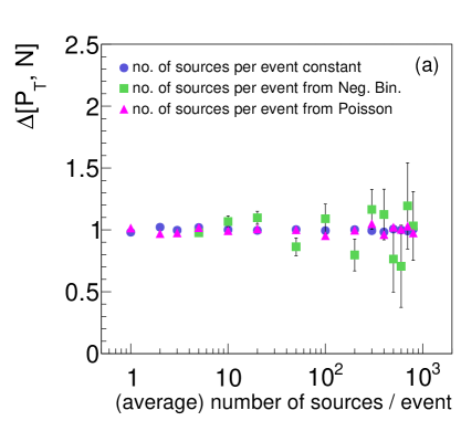
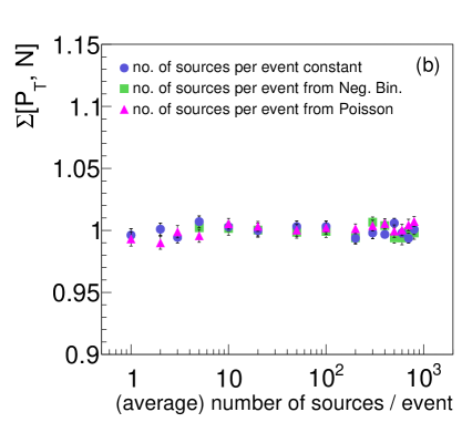
The first set of the MC simulations refers to particle production from sources with fixed temperature. For each source in a given event the number of particles was generated from the Poisson distribution with a mean value of 5. The particle transverse momentum was generated from transverse momentum distribution (33) with maximal value pmax=2.0subscript𝑝max2.0p_{{\rm max}}=2.0 GeV/c𝑐c. The temperature parameter is fixed as T=150𝑇150T=150 MeV. The number of sources NSsubscript𝑁𝑆N_{S} composing an event is either constant (circles in Fig. 1) or selected from Poisson (triangles) or from Negative Binomial distribution (squares). For Negative Binomial distribution its dispersion Var(NS)𝑉𝑎𝑟subscript𝑁𝑆\sqrt{Var(N_{S})} is large and equals NS/2delimited-⟨⟩subscript𝑁𝑆2\langle N_{S}\rangle/2.

Refer to caption
Refer to caption
Figure 1: (Color online) The symbols are the MC results for the Δ[PT,N]Δsubscript𝑃𝑇𝑁\Delta[P_{T},N] (a) and Σ[PT,N]Σsubscript𝑃𝑇𝑁\Sigma[P_{T},N] (b) measures versus the number or mean number of sources composing one event. All sources have fixed temperature. The number of sources per event are fixed (circles) or fluctuating according to the Poisson distribution (triangles) and Negative Binomial distribution (squares).

Figure 1 shows Δ[PT,N]Δsubscript𝑃𝑇𝑁\Delta[P_{T},N] and Σ[PT,N]Σsubscript𝑃𝑇𝑁\Sigma[P_{T},N] versus the number or the mean number of sources composing one event. The distribution function of a single source has the form of Eq. (28) and the PS(x)subscript𝑃𝑆𝑥P_{S}(x) function is taken as f(p,T)𝑓𝑝𝑇f(p,T) (33) with fixed temperature T𝑇T, same for all sources. This corresponds the case when the MIS is reduced to the IPM, and relation (14) should be valid. As expected, the Δ[PT,N]Δsubscript𝑃𝑇𝑁\Delta[P_{T},N] and Σ[PT,N]Σsubscript𝑃𝑇𝑁\Sigma[P_{T},N] values for the MC simulations are consistent with one, independently of the assumed shape of transverse momentum distribution. The circles in Fig. 1 confirm that Δ[PT,N]Δsubscript𝑃𝑇𝑁\Delta[P_{T},N] and Σ[PT,N]Σsubscript𝑃𝑇𝑁\Sigma[P_{T},N] are intensive measures (do not depend on NSsubscript𝑁𝑆N_{S}), whereas the triangles and the squares show that these quantities are also strongly intensive (do not depend on NSsubscript𝑁𝑆N_{S} fluctuations).

For a constant number of sources per event (circles in Fig. 1), the scaled variance of multiplicity distribution ω[N]=ω[n]+n¯ω[NS]𝜔delimited-[]𝑁𝜔delimited-[]𝑛¯𝑛𝜔delimited-[]subscript𝑁𝑆\omega[N]=\omega[n]+\overline{n}\omega[N_{S}] equals 1 in the whole range of the horizontal axis. For the Poisson distribution of the number of sources ω[N]𝜔delimited-[]𝑁\omega[N] equals to 6 also for the whole range of the mean number of sources per event. For the Negative Binomial distribution of the number of sources ω[N]𝜔delimited-[]𝑁\omega[N] increases from about 7 at NS=5delimited-⟨⟩subscript𝑁𝑆5\langle N_{S}\rangle=5, through 126 at NS=100delimited-⟨⟩subscript𝑁𝑆100\langle N_{S}\rangle=100, up to approximately 1000 at NS=800delimited-⟨⟩subscript𝑁𝑆800\langle N_{S}\rangle=800. Therefore, Fig. 1 shows that Δ[PT,N]Δsubscript𝑃𝑇𝑁\Delta[P_{T},N] and Σ[PT,N]Σsubscript𝑃𝑇𝑁\Sigma[P_{T},N] measures are strongly intensive even for multiplicity distributions which are extremely wide.

III.2 Source Temperature Fluctuations

In the next set of simulations, the number of particles produced by each single source is again selected from the Poisson distribution with a mean value of n¯=5¯𝑛5\overline{n}=5. The particle transverse momentum is generated by the transverse momentum distribution (33) with average inverse slope parameter T¯=150¯𝑇150\overline{T}=150 MeV. The T𝑇T parameter is generated separately for each single source (source-by-source T𝑇T fluctuations) from the Gaussian distribution

W(T)=12πσTexp[(TT¯)22σT2],𝑊𝑇12𝜋subscript𝜎𝑇superscript𝑇¯𝑇22superscriptsubscript𝜎𝑇2\displaystyle W(T)\leavevmode\nobreak\ =\leavevmode\nobreak\ \frac{1}{\sqrt{2\pi}\,\sigma_{T}}\exp\Big{[}\,-\leavevmode\nobreak\ \frac{(T-\overline{T})^{2}}{2\sigma_{T}^{2}}\Big{]}\leavevmode\nobreak\ , (39)

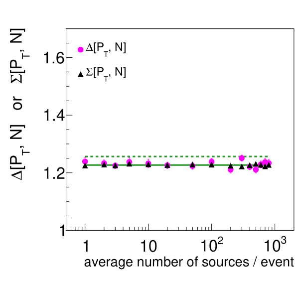
with dispersion σT=25subscript𝜎𝑇25\sigma_{T}=25 MeV. Finally, the number of sources NSsubscript𝑁𝑆N_{S} composing an event is generated from the Poisson distribution, with NSdelimited-⟨⟩subscript𝑁𝑆\langle N_{S}\rangle as denoted on the horizontal axis of Fig. 2. As seen, the effect of source temperature fluctuations results in Δ[PT,N]Δsubscript𝑃𝑇𝑁\Delta[P_{T},N] and Σ[PT,N]Σsubscript𝑃𝑇𝑁\Sigma[P_{T},N] values higher than 1.

If the parameter T𝑇T fluctuates independently for each source, the sources remain to be statistically identical and independent of each other. Therefore, these MC simulations correspond to the MIS and the Δ[PT,N]Δsubscript𝑃𝑇𝑁\Delta[P_{T},N] and Σ[PT,N]Σsubscript𝑃𝑇𝑁\Sigma[P_{T},N] strongly intensive measures should not depend on the mean number of sources NSdelimited-⟨⟩subscript𝑁𝑆\langle N_{S}\rangle and on its fluctuations ω[NS]𝜔delimited-[]subscript𝑁𝑆\omega[N_{S}]. Indeed, Fig. 2 confirms this expectation.
Refer to caption
Figure 2: (Color online) The symbols are the MC results for the Δ[PT,N]Δsubscript𝑃𝑇𝑁\Delta[P_{T},N] (circles) and Σ[PT,N]Σsubscript𝑃𝑇𝑁\Sigma[P_{T},N] (triangles) measures versus the mean number of sources composing one event. The temperatures of the sources fluctuate independently according to Eq. (39), and the number of sources per event fluctuates according to the Poisson distribution. The solid line corresponds to Eq. (48), the dashed line to Eq. (51).

The distribution function of a single source has the form of Eq. (30) with FS(x,T)subscript𝐹𝑆𝑥𝑇F_{S}(x,T) function taken as f(p,T)𝑓𝑝𝑇f(p,T). This leads to the result (PPT𝑃subscript𝑃𝑇P\equiv P_{T}) (32)

Δ[P,N]=Σ[P,N]=ω[PS]p¯ω[n]ω[p],ω[p]p2¯p¯2p¯.formulae-sequenceΔ𝑃𝑁Σ𝑃𝑁𝜔delimited-[]subscript𝑃𝑆¯𝑝𝜔delimited-[]𝑛𝜔delimited-[]𝑝𝜔delimited-[]𝑝¯superscript𝑝2superscript¯𝑝2¯𝑝\displaystyle\Delta[P,N]\leavevmode\nobreak\ =\leavevmode\nobreak\ \Sigma[P,N]\leavevmode\nobreak\ =\leavevmode\nobreak\ \frac{\omega[P_{S}]\leavevmode\nobreak\ -\leavevmode\nobreak\ \overline{p}\cdot\omega[n]}{\omega[p]}\leavevmode\nobreak\ ,\leavevmode\nobreak\ \leavevmode\nobreak\ \leavevmode\nobreak\ \leavevmode\nobreak\ \omega[p]\leavevmode\nobreak\ \equiv\leavevmode\nobreak\ \frac{\overline{p^{2}}\leavevmode\nobreak\ -\leavevmode\nobreak\ \overline{p}^{2}}{\overline{p}}. (40)

For PS¯¯subscript𝑃𝑆\overline{P_{S}} and PS2¯¯superscriptsubscript𝑃𝑆2\overline{P_{S}^{2}} one obtains:

PS¯=p¯n¯,¯subscript𝑃𝑆¯𝑝¯𝑛\displaystyle\overline{P_{S}}\leavevmode\nobreak\ =\leavevmode\nobreak\ \overline{p}\cdot\overline{n}\leavevmode\nobreak\ , (41)
(PS)2¯=n𝒫S(n)𝑑TW(T)0i=1n[pidpif(pi)](p1++pn)2¯superscriptsubscript𝑃𝑆2subscript𝑛subscript𝒫𝑆𝑛differential-d𝑇𝑊𝑇superscriptsubscript0superscriptsubscriptproduct𝑖1𝑛delimited-[]subscript𝑝𝑖𝑑subscript𝑝𝑖𝑓subscript𝑝𝑖superscriptsubscript𝑝1subscript𝑝𝑛2\displaystyle\overline{(P_{S})^{2}}\leavevmode\nobreak\ =\leavevmode\nobreak\ \sum_{n}{\cal P}_{S}(n)\leavevmode\nobreak\ \int dTW(T)\leavevmode\nobreak\ \int_{0}^{\infty}\prod_{i=1}^{n}\Big{[}p_{i}dp_{i}\,f(p_{i})\Big{]}\leavevmode\nobreak\ (p_{1}+\ldots+p_{n})^{2}\leavevmode\nobreak\
=n𝒫S(n)𝑑TW(T)0i=1n[pidpif(pi)][j=1npj2+1lmkplpm]absentsubscript𝑛subscript𝒫𝑆𝑛differential-d𝑇𝑊𝑇superscriptsubscript0superscriptsubscriptproduct𝑖1𝑛delimited-[]subscript𝑝𝑖𝑑subscript𝑝𝑖𝑓subscript𝑝𝑖delimited-[]superscriptsubscript𝑗1𝑛superscriptsubscript𝑝𝑗2subscript1𝑙𝑚𝑘subscript𝑝𝑙subscript𝑝𝑚\displaystyle=\leavevmode\nobreak\ \sum_{n}{\cal P}_{S}(n)\leavevmode\nobreak\ \int dTW(T)\leavevmode\nobreak\ \int_{0}^{\infty}\prod_{i=1}^{n}\Big{[}p_{i}dp_{i}\,f(p_{i})\Big{]}\leavevmode\nobreak\ \Big{[}\sum_{j=1}^{n}p_{j}^{2}\leavevmode\nobreak\ +\sum_{1\leq l\neq m\leq k}p_{l}\cdot p_{m}\Big{]}
=n𝒫S(k)𝑑TW(T)[np2~+n(n1)p~2]=p2¯n¯+p^2[n2¯n¯],absentsubscript𝑛subscript𝒫𝑆𝑘differential-d𝑇𝑊𝑇delimited-[]𝑛~superscript𝑝2𝑛𝑛1superscript~𝑝2¯superscript𝑝2¯𝑛superscript^𝑝2delimited-[]¯superscript𝑛2¯𝑛\displaystyle=\leavevmode\nobreak\ \sum_{n}{\cal P}_{S}(k)\leavevmode\nobreak\ \int dTW(T)\leavevmode\nobreak\ \Big{[}n\cdot\tilde{p^{2}}\leavevmode\nobreak\ +\leavevmode\nobreak\ n(n-1)\cdot\tilde{p}^{2}\Big{]}\leavevmode\nobreak\ =\leavevmode\nobreak\ \overline{p^{2}}\cdot\overline{n}\leavevmode\nobreak\ +\leavevmode\nobreak\ \hat{p}^{2}\cdot\Big{[}\overline{n^{2}}\leavevmode\nobreak\ -\leavevmode\nobreak\ \overline{n}\Big{]}\leavevmode\nobreak\ , (42)

where

p^2𝑑TW(T)p~2.superscript^𝑝2differential-d𝑇𝑊𝑇superscript~𝑝2\displaystyle\hat{p}^{2}\leavevmode\nobreak\ \equiv\leavevmode\nobreak\ \int dT\,W(T)\leavevmode\nobreak\ \tilde{p}^{2}\leavevmode\nobreak\ . (43)

Calculating ω[PS]𝜔delimited-[]subscript𝑃𝑆\omega[P_{S}] from Eqs. (41,42) and inserting it into Eq. (32) one obtains:

Δ[P,N]=Σ[P,N]= 1+1ω[p]p^2p¯2p¯[n¯+ω[n] 1].Δ𝑃𝑁Σ𝑃𝑁11𝜔delimited-[]𝑝superscript^𝑝2superscript¯𝑝2¯𝑝delimited-[]¯𝑛𝜔delimited-[]𝑛1\displaystyle\Delta[P,N]\leavevmode\nobreak\ =\leavevmode\nobreak\ \Sigma[P,N]\leavevmode\nobreak\ =\leavevmode\nobreak\ 1\leavevmode\nobreak\ +\leavevmode\nobreak\ \frac{1}{\omega[p]}\cdot\frac{\hat{p}^{2}\leavevmode\nobreak\ -\leavevmode\nobreak\ \overline{p}^{2}}{\overline{p}}\cdot\Big{[}\overline{n}\leavevmode\nobreak\ +\leavevmode\nobreak\ \omega[n]\leavevmode\nobreak\ -\leavevmode\nobreak\ 1\Big{]}\leavevmode\nobreak\ . (44)

One can easily prove that

p^2p¯2=𝑑TW(T)(p~p¯)2 0,superscript^𝑝2superscript¯𝑝2differential-d𝑇𝑊𝑇superscript~𝑝¯𝑝2 0\displaystyle\hat{p}^{2}\leavevmode\nobreak\ -\leavevmode\nobreak\ \overline{p}^{2}\leavevmode\nobreak\ =\leavevmode\nobreak\ \int dT\,W(T)\leavevmode\nobreak\ (\tilde{p}\leavevmode\nobreak\ -\leavevmode\nobreak\ \overline{p})^{2}\leavevmode\nobreak\ \geq\leavevmode\nobreak\ 0\leavevmode\nobreak\ , (45)
n¯+ω[n] 1=n2¯n¯n¯=1n¯n2𝒫S(n)(n2n) 0.¯𝑛𝜔delimited-[]𝑛1¯superscript𝑛2¯𝑛¯𝑛1¯𝑛subscript𝑛2subscript𝒫𝑆𝑛superscript𝑛2𝑛 0\displaystyle\overline{n}\leavevmode\nobreak\ +\leavevmode\nobreak\ \omega[n]\leavevmode\nobreak\ -\leavevmode\nobreak\ 1\leavevmode\nobreak\ =\leavevmode\nobreak\ \frac{\overline{n^{2}}\leavevmode\nobreak\ -\leavevmode\nobreak\ \overline{n}}{\overline{n}}\leavevmode\nobreak\ =\leavevmode\nobreak\ \frac{1}{\overline{n}}\leavevmode\nobreak\ \sum_{n\geq 2}{\cal P}_{S}(n)\,(n^{2}\leavevmode\nobreak\ -\leavevmode\nobreak\ n)\leavevmode\nobreak\ \geq\leavevmode\nobreak\ 0\leavevmode\nobreak\ . (46)

When temperature fluctuations are absent, relation (45) is transformed to p^2p¯2=0superscript^𝑝2superscript¯𝑝20\hat{p}^{2}-\overline{p}^{2}=0, and Eq. (44) is reduced to Eq. (14). The same happens when 𝒫S(n)=0subscript𝒫𝑆𝑛0{\cal P}_{S}(n)=0 for all n2𝑛2n\geq 2, and, thus, n¯+ω[n]1=0¯𝑛𝜔delimited-[]𝑛10\overline{n}+\omega[n]-1=0. This is intuitively clear: the MIS is reduced to the IPM if each source can emit only one or zero number of particles.

In Fig. 2 the results of the MC simulations are compared with analytical results of Eq. (44). The solid line corresponds to the distribution (33) and Gaussian temperature fluctuations (39). In this case one finds:

p¯0.328GeV/c,p2¯0.158(GeV/c)2,p^20.110(GeV/c)2.formulae-sequence¯𝑝0.328GeV𝑐formulae-sequence¯superscript𝑝20.158superscriptGeV𝑐2superscript^𝑝20.110superscriptGeV𝑐2\displaystyle\overline{p}\cong 0.328\leavevmode\nobreak\ {\rm GeV}/c\leavevmode\nobreak\ ,\leavevmode\nobreak\ \leavevmode\nobreak\ \leavevmode\nobreak\ \leavevmode\nobreak\ \overline{p^{2}}\cong 0.158\leavevmode\nobreak\ ({\rm GeV}/c)^{2}\leavevmode\nobreak\ ,\leavevmode\nobreak\ \leavevmode\nobreak\ \leavevmode\nobreak\ \leavevmode\nobreak\ \hat{p}^{2}\cong 0.110\leavevmode\nobreak\ ({\rm GeV}/c)^{2}\leavevmode\nobreak\ . (47)

The 𝒫S(n)subscript𝒫𝑆𝑛{\cal P}_{S}(n) Poisson distribution for a single source corresponds to n¯=5¯𝑛5\overline{n}=5 and ω[n]=1𝜔delimited-[]𝑛1\omega[n]=1, therefore, n¯+ω[n]1=5¯𝑛𝜔delimited-[]𝑛15\overline{n}+\omega[n]-1=5. The final result of Eq. (44) is

Δ[P,N]=Σ[P,N]1.227.Δ𝑃𝑁Σ𝑃𝑁1.227\displaystyle\Delta[P,N]\leavevmode\nobreak\ =\leavevmode\nobreak\ \Sigma[P,N]\leavevmode\nobreak\ \cong 1.227\leavevmode\nobreak\ . (48)

As seen in Fig. 2, this is in a good agreement with the results of the MC simulations.

For massless particles the quantities in Eq. (47) can be calculated analytically

p¯= 2T¯= 0.3GeV/c,p2¯=6T2¯= 6[T¯2+σT2]= 0.13875(GeV/c)2,formulae-sequence¯𝑝2¯𝑇0.3GeV𝑐¯superscript𝑝26¯superscript𝑇26delimited-[]superscript¯𝑇2subscriptsuperscript𝜎2𝑇0.13875superscriptGeV𝑐2\displaystyle\overline{p}\leavevmode\nobreak\ =\leavevmode\nobreak\ 2\overline{T}\leavevmode\nobreak\ =\leavevmode\nobreak\ 0.3\leavevmode\nobreak\ {\rm GeV}/c\leavevmode\nobreak\ ,\leavevmode\nobreak\ \leavevmode\nobreak\ \leavevmode\nobreak\ \leavevmode\nobreak\ \leavevmode\nobreak\ \leavevmode\nobreak\ \leavevmode\nobreak\ \leavevmode\nobreak\ \overline{p^{2}}=6\overline{T^{2}}\leavevmode\nobreak\ =\leavevmode\nobreak\ 6\,[\overline{T}^{2}\leavevmode\nobreak\ +\leavevmode\nobreak\ \sigma^{2}_{T}]\leavevmode\nobreak\ =\leavevmode\nobreak\ 0.13875\leavevmode\nobreak\ ({\rm GeV}/c)^{2},\leavevmode\nobreak\ \leavevmode\nobreak\ \leavevmode\nobreak\ \leavevmode\nobreak\ (49)
p2^=𝑑TW(T)p~2= 4T2¯=4[T¯2+σT2]= 0.0925(GeV/c)2.^superscript𝑝2differential-d𝑇𝑊𝑇superscript~𝑝24¯superscript𝑇24delimited-[]superscript¯𝑇2superscriptsubscript𝜎𝑇20.0925superscriptGeV𝑐2\displaystyle\hat{p^{2}}\leavevmode\nobreak\ =\leavevmode\nobreak\ \int dT\,W(T)\,\tilde{p}^{2}\leavevmode\nobreak\ =\leavevmode\nobreak\ 4\overline{T^{2}}\leavevmode\nobreak\ =4[\overline{T}^{2}\leavevmode\nobreak\ +\leavevmode\nobreak\ \sigma_{T}^{2}]\leavevmode\nobreak\ =\leavevmode\nobreak\ 0.0925\leavevmode\nobreak\ ({\rm GeV}/c)^{2}\leavevmode\nobreak\ . (50)

With Eqs. (49,50) one finds

Δ[P,N]=Σ[P,N]= 1+2σT2T¯2+3σT2[n¯+ω[n] 1].Δ𝑃𝑁Σ𝑃𝑁12superscriptsubscript𝜎𝑇2superscript¯𝑇23superscriptsubscript𝜎𝑇2delimited-[]¯𝑛𝜔delimited-[]𝑛1\displaystyle\Delta[P,N]\leavevmode\nobreak\ =\leavevmode\nobreak\ \Sigma[P,N]\leavevmode\nobreak\ =\leavevmode\nobreak\ 1\leavevmode\nobreak\ +\leavevmode\nobreak\ \frac{2\sigma_{T}^{2}}{\overline{T}^{2}+3\sigma_{T}^{2}}\cdot\Big{[}\overline{n}\leavevmode\nobreak\ +\leavevmode\nobreak\ \omega[n]\leavevmode\nobreak\ -\leavevmode\nobreak\ 1\Big{]}\leavevmode\nobreak\ . (51)

For the values T¯=0.15¯𝑇0.15\overline{T}=0.15 GeV, σT=0.025subscript𝜎𝑇0.025\sigma_{T}=0.025 GeV, n¯=5¯𝑛5\overline{n}=5, and ω[n]=1𝜔delimited-[]𝑛1\omega[n]=1 used in the MC simulations one finds Δ[P,N]=Σ[P,N]1.256Δ𝑃𝑁Σ𝑃𝑁1.256\Delta[P,N]=\Sigma[P,N]\cong 1.256. This result for m=0𝑚0m=0 is shown in Fig. 2 by the dashed line.

The MC results presented in Figs. 1 and 2 demonstrate a different sensitivity of the strongly intensive measures to model details: despite of the equality Δ[PT,N]=Σ[PT,N]Δsubscript𝑃𝑇𝑁Σsubscript𝑃𝑇𝑁\Delta[P_{T},N]=\Sigma[P_{T},N] the statistical errors of the simulations calculated for Δ[PT,N]Δsubscript𝑃𝑇𝑁\Delta[P_{T},N] are found to be essentially larger than those for Σ[PT,N]Σsubscript𝑃𝑇𝑁\Sigma[P_{T},N] 111In order to avoid too large statistical errors, in Fig. 2 we used five times higher statistics (500k events for each point) than that one used in Figs. 1 and 3..

III.3 Global Temperature Fluctuations

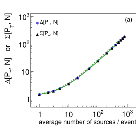
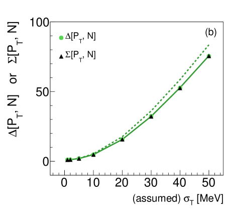
In the next MC simulations, source-by-source T𝑇T fluctuations from the previous subsection are replaced by e-by-e (global) T𝑇T fluctuations. The parameter T𝑇T is the same for all sources composing a given event but is varied between events following the Gaussian distribution (39) with average inverse slope parameter T=150delimited-⟨⟩𝑇150\langle T\rangle=150 MeV and dispersion σTsubscript𝜎𝑇\sigma_{T}. The number of sources NSsubscript𝑁𝑆N_{S} composing an event is generated from the Poisson distribution with NSdelimited-⟨⟩subscript𝑁𝑆\langle N_{S}\rangle being the average value. As previously, for each single source, the number of particles was selected from the Poisson distribution with a mean value of n¯=5¯𝑛5\overline{n}=5. The results are presented in Fig. 3. Its (a) panel shows the dependence of Δ[PT,N]Δsubscript𝑃𝑇𝑁\Delta[P_{T},N] and Σ[PT,N]Σsubscript𝑃𝑇𝑁\Sigma[P_{T},N]) on the average number of sources NSdelimited-⟨⟩subscript𝑁𝑆\langle N_{S}\rangle at σT=25subscript𝜎𝑇25\sigma_{T}=25 MeV, whereas the (b) panel presents the dependence on σTsubscript𝜎𝑇\sigma_{T} at NS=100delimited-⟨⟩subscript𝑁𝑆100\langle N_{S}\rangle=100. In Fig. 3 (b) in order to avoid negative T𝑇T values only events within T=150±3σT𝑇plus-or-minus1503subscript𝜎𝑇T=150\pm 3\sigma_{T} MeV were accepted. We also would like to mention here that the relationship between temperature and multiplicity (or volume) fluctuations was studied in Refs. volume ; multip_T_fluct .

Due to the correlated T𝑇T-fluctuations for different sources, the sources are not independent of each other. Therefore, these MC simulations do not correspond to the MIS. One can nevertheless use the formula from the previous subsection with the following substitutions:

NS1,ω[NS]0,nN,PSP,formulae-sequencesubscript𝑁𝑆1formulae-sequence𝜔delimited-[]subscript𝑁𝑆0formulae-sequence𝑛𝑁subscript𝑃𝑆𝑃\displaystyle N_{S}\rightarrow 1\leavevmode\nobreak\ ,\leavevmode\nobreak\ \leavevmode\nobreak\ \leavevmode\nobreak\ \leavevmode\nobreak\ \omega[N_{S}]\rightarrow 0\leavevmode\nobreak\ ,\leavevmode\nobreak\ \leavevmode\nobreak\ \leavevmode\nobreak\ \leavevmode\nobreak\ n\rightarrow N\leavevmode\nobreak\ ,\leavevmode\nobreak\ \leavevmode\nobreak\ \leavevmode\nobreak\ \leavevmode\nobreak\ P_{S}\rightarrow P\leavevmode\nobreak\ , (52)

i.e. all final particles are treated as created from a “single source” with fluctuating temperature T𝑇T. Note that the parameter T𝑇T becomes an event variable with average value T=T¯=150delimited-⟨⟩𝑇¯𝑇150\langle T\rangle=\overline{T}=150 MeV and distribution (39). This gives:

Δ[P,N]=Σ[P,N]= 1+1ω[p]p^2p¯2p¯[N+ω[N] 1].Δ𝑃𝑁Σ𝑃𝑁11𝜔delimited-[]𝑝superscript^𝑝2superscript¯𝑝2¯𝑝delimited-[]delimited-⟨⟩𝑁𝜔delimited-[]𝑁1\displaystyle\Delta[P,N]\leavevmode\nobreak\ =\leavevmode\nobreak\ \Sigma[P,N]\leavevmode\nobreak\ =\leavevmode\nobreak\ 1\leavevmode\nobreak\ +\leavevmode\nobreak\ \frac{1}{\omega[p]}\cdot\frac{\hat{p}^{2}\leavevmode\nobreak\ -\leavevmode\nobreak\ \overline{p}^{2}}{\overline{p}}\cdot\Big{[}\,\langle N\rangle\leavevmode\nobreak\ +\leavevmode\nobreak\ \omega[N]\leavevmode\nobreak\ -\leavevmode\nobreak\ 1\,\Big{]}\leavevmode\nobreak\ . (53)
Refer to caption
Refer to caption
Figure 3: (Color online) The symbols are the MC results for the Δ[PT,N]Δsubscript𝑃𝑇𝑁\Delta[P_{T},N] (circles) and Σ[PT,N]Σsubscript𝑃𝑇𝑁\Sigma[P_{T},N] (triangles) measures. The MC simulations correspond to the global temperature fluctuations according to Eq. (39), i.e. temperatures of all sources are equal. The number of sources are taken from the Poisson distribution with the average value of NSdelimited-⟨⟩subscript𝑁𝑆\langle N_{S}\rangle. The solid lines present the results of Eq. (53), the dashed lines of Eq. (55). (a): The dependence on the mean number of sources at fixed σT=25subscript𝜎𝑇25\sigma_{T}=25 MeV. (b): The dependence on σTsubscript𝜎𝑇\sigma_{T} at fixed NS=100delimited-⟨⟩subscript𝑁𝑆100\langle N_{S}\rangle=100 (here for calculating dashed line the obtained σTsubscript𝜎𝑇\sigma_{T} values were used; due to the limited range of T𝑇T distribution they are slightly smaller than the assumed ones).

The MC results on global temperature fluctuations are compared to analytical predictions of Eq. (53). The solid lines in Fig. 3 correspond to the transverse momentum distribution (33) with temperature fluctuating according to Eq. (39). The values of p¯¯𝑝\overline{p}, p2¯¯superscript𝑝2\overline{p^{2}}, p^2superscript^𝑝2\hat{p}^{2}, and ω[p]𝜔delimited-[]𝑝\omega[p] are calculated numerically with Eqs. (33) and (39). At σT=25subscript𝜎𝑇25\sigma_{T}=25 MeV, they are equal to those in Eq. (47). Analytical calculations can be done for massless particles according to Eq. (49) which demonstrates the explicit dependence on σTsubscript𝜎𝑇\sigma_{T}.

Note that multiplicities n1,,nNSsubscript𝑛1subscript𝑛subscript𝑁𝑆n_{1},\dots,n_{N_{S}} for particles emitted by different sources are uncorrelated. Therefore, one can use the MIS to calculate Ndelimited-⟨⟩𝑁\langle N\rangle and ω[N]𝜔delimited-[]𝑁\omega[N] with Eq. (24):

N=n¯NS=5NS,ω[N]=ω[n]+n¯ω[NS]=1+51=6.formulae-sequencedelimited-⟨⟩𝑁¯𝑛delimited-⟨⟩subscript𝑁𝑆5delimited-⟨⟩subscript𝑁𝑆𝜔delimited-[]𝑁𝜔delimited-[]𝑛¯𝑛𝜔delimited-[]subscript𝑁𝑆1516\displaystyle\langle N\rangle=\overline{n}\langle N_{S}\rangle=5\langle N_{S}\rangle\leavevmode\nobreak\ ,\leavevmode\nobreak\ \leavevmode\nobreak\ \leavevmode\nobreak\ \leavevmode\nobreak\ \omega[N]=\omega[n]+\overline{n}\cdot\omega[N_{S}]=1+5\cdot 1=6\leavevmode\nobreak\ . (54)

This results in a linear increase of (53) with NSdelimited-⟨⟩subscript𝑁𝑆\langle N_{S}\rangle.

For m=0𝑚0m=0 in the distribution (33), similarly to Eq. (51), one obtains

Δ[P,N]=Σ[P,N]= 1+2σT2T2+3σT2[5Ns+ 5],Δ𝑃𝑁Σ𝑃𝑁12superscriptsubscript𝜎𝑇2superscriptdelimited-⟨⟩𝑇23superscriptsubscript𝜎𝑇2delimited-[]5delimited-⟨⟩subscript𝑁𝑠5\displaystyle\Delta[P,N]\leavevmode\nobreak\ =\leavevmode\nobreak\ \Sigma[P,N]\leavevmode\nobreak\ =\leavevmode\nobreak\ 1\leavevmode\nobreak\ +\leavevmode\nobreak\ \frac{2\sigma_{T}^{2}}{\langle T\rangle^{2}+3\sigma_{T}^{2}}\cdot\Big{[}5\,\langle N_{s}\rangle\leavevmode\nobreak\ +\leavevmode\nobreak\ 5\Big{]}\leavevmode\nobreak\ , (55)

where Eq. (54) has been already used. This is shown in Fig. 3 by dashed lines.

As expected from Eq. (53), the fluctuation measures Δ[PT,N]Δsubscript𝑃𝑇𝑁\Delta[P_{T},N] and Σ[PT,N]Σsubscript𝑃𝑇𝑁\Sigma[P_{T},N]) increase when global temperature fluctuations are stronger (higher σTsubscript𝜎𝑇\sigma_{T}). This is explicitly seen from Eq. (55) for m=0𝑚0m=0. The same conclusion was drawn in Ref. m8 , where the influence of temperature fluctuations on transverse momentum fluctuations was studied for the ΦpTsubscriptΦsubscript𝑝𝑇\Phi_{p_{T}} measure GM:1992 (see also Ref. KG:APP2012 for the corresponding plot).

IV Temperature Correlations Versus Number of Particles

The results of fast generators in the previous section showed the same behavior and magnitudes of Δ[PT,N]Δsubscript𝑃𝑇𝑁\Delta[P_{T},N] and Σ[PT,N]Σsubscript𝑃𝑇𝑁\Sigma[P_{T},N] measures. The MC simulation, presented in this section, is introduced in order to check whether one can propose a fast generator for which different values of Δ[PT,N]Δsubscript𝑃𝑇𝑁\Delta[P_{T},N] and Σ[PT,N]Σsubscript𝑃𝑇𝑁\Sigma[P_{T},N] may be obtained. As an example, we consider the M(pT)𝑀subscript𝑝𝑇M(p_{T}) versus N𝑁N correlation suggested in Ref. GM:1992 , where M(pT)𝑀subscript𝑝𝑇M(p_{T}) is the event mean single-particle transverse momentum and N𝑁N is the particle multiplicity. In Fig. 4 (a) the assumed multiplicity distribution is presented as red triangles (those values correspond to the accepted multiplicities at forward rapidities in p+p𝑝𝑝p+p collisions at the beam energy 158 GeV d1 ). As seen, the generated multiplicity distribution (gray histogram) coincides with the assumed one. For each event, particle momenta are generated from transverse momentum distribution (33) with T𝑇T taken as TN=M(pT)N/2subscript𝑇𝑁subscriptdelimited-⟨⟩𝑀subscript𝑝𝑇𝑁2T_{N}=\langle M(p_{T})\rangle_{N}/2, where M(pT)Nsubscriptdelimited-⟨⟩𝑀subscript𝑝𝑇𝑁\langle M(p_{T})\rangle_{N} is dependent on generated multiplicity N𝑁N as shown in Fig. 4 (b) by the red triangles d1 . The range of pTsubscript𝑝𝑇p_{T} generation is from zero to 2 GeV/c𝑐c. In Fig. 4 (b) the scatter plot represents all generated events (M(pT)𝑀subscript𝑝𝑇M(p_{T}) values) and the gray squares their profile histogram (M(pT)Nsubscriptdelimited-⟨⟩𝑀subscript𝑝𝑇𝑁\langle M(p_{T})\rangle_{N} values, where Nsubscriptdelimited-⟨⟩𝑁\langle...\rangle_{N} represents averaging within the same multiplicity N𝑁N). The difference between red triangles (input values of 2TN2subscript𝑇𝑁2\,T_{N} used in simulation) and gray squares (M(pT)Nsubscriptdelimited-⟨⟩𝑀subscript𝑝𝑇𝑁\langle M(p_{T})\rangle_{N} values obtained from simulated data set) is due to the fact that in transverse momentum distribution used in simulation (33) the average transverse momentum is only approximately equal to 2T2𝑇2\,T. It was, however, verified by an independent analysis that when using f(p,T)=Cpexp(p/T)𝑓𝑝𝑇𝐶𝑝𝑝𝑇f(p,T)=C\,p\,\exp(-p/T) distribution, for which the mean transverse momentum equals exactly 2T2𝑇2\,T, red and gray points coincide. For the simulation presented in Fig. 4 the values of fluctuation measures obtained for 500 000 generated events are:

Δ[PT,N]= 0.8158± 0.0051,Σ[PT,N]= 1.0075± 0.0018.formulae-sequenceΔsubscript𝑃𝑇𝑁plus-or-minus0.81580.0051Σsubscript𝑃𝑇𝑁plus-or-minus1.00750.0018\displaystyle\Delta[P_{T},N]\leavevmode\nobreak\ =\leavevmode\nobreak\ 0.8158\leavevmode\nobreak\ \pm\leavevmode\nobreak\ 0.0051\leavevmode\nobreak\ ,\leavevmode\nobreak\ \leavevmode\nobreak\ \leavevmode\nobreak\ \leavevmode\nobreak\ \Sigma[P_{T},N]\leavevmode\nobreak\ =\leavevmode\nobreak\ 1.0075\leavevmode\nobreak\ \pm\leavevmode\nobreak\ 0.0018\leavevmode\nobreak\ . (56)
Refer to caption
Figure 4: (Color online) Properties of the fast generator producing M(pT)𝑀subscript𝑝𝑇M(p_{T}) versus N𝑁N correlation (see the text for details). Green solid line (b) shows Eqs. (69, 70), where Ndelimited-⟨⟩𝑁\langle N\rangle = 1.4 and TN=M(pT)N/2subscript𝑇𝑁subscriptdelimited-⟨⟩𝑀subscript𝑝𝑇𝑁2T_{N}=\langle M(p_{T})\rangle_{N}/2.

Particle production considered in this section corresponds to the distribution

FN(p1,,pN)=𝒫(N)×fN(p1)××fN(pN)subscript𝐹𝑁subscript𝑝1subscript𝑝𝑁𝒫𝑁subscript𝑓𝑁subscript𝑝1subscript𝑓𝑁subscript𝑝𝑁\displaystyle F_{N}(p_{1},\dots,p_{N})\leavevmode\nobreak\ =\leavevmode\nobreak\ {\cal P}(N)\times f_{N}(p_{1})\times\dots\times f_{N}(p_{N}) (57)

where fN(p)=f(p,TN)subscript𝑓𝑁𝑝𝑓𝑝subscript𝑇𝑁f_{N}(p)=f(p,T_{N}) with f(p,TN)𝑓𝑝subscript𝑇𝑁f(p,T_{N}) given by Eq. (33), but with the parameter T𝑇T depending now on the particle multiplicity, TN=T(N)subscript𝑇𝑁𝑇𝑁T_{N}=T(N). The moments of single particle distributions at fixed N𝑁N are then equal to

(pk¯)N=0𝑑ppkfN(p).subscript¯superscript𝑝𝑘𝑁superscriptsubscript0differential-d𝑝superscript𝑝𝑘subscript𝑓𝑁𝑝\displaystyle(\overline{p^{k}})_{N}\leavevmode\nobreak\ =\leavevmode\nobreak\ \int_{0}^{\infty}dp\leavevmode\nobreak\ p^{k}\leavevmode\nobreak\ f_{N}(p)\leavevmode\nobreak\ . (58)

The moments of single particle spectrum averaged over N𝑁N are

pk¯=NN𝒫(N)N(pk¯)N,¯superscript𝑝𝑘subscript𝑁𝑁𝒫𝑁delimited-⟨⟩𝑁subscript¯superscript𝑝𝑘𝑁\displaystyle\overline{p^{k}}\leavevmode\nobreak\ =\leavevmode\nobreak\ \sum_{N}\frac{N\,{\cal P}(N)}{\langle N\rangle}\leavevmode\nobreak\ (\overline{p^{k}})_{N}\leavevmode\nobreak\ , (59)

and ω[p]=(p2¯p¯2)/p¯𝜔delimited-[]𝑝¯superscript𝑝2superscript¯𝑝2¯𝑝\omega[p]=(\overline{p^{2}}\leavevmode\nobreak\ -\leavevmode\nobreak\ \overline{p}^{2})/\overline{p} .

With distribution (57) one finds:

P=N𝒫(N)fN(p1)𝑑p1fN(pN)𝑑pN(p1++pN)delimited-⟨⟩𝑃subscript𝑁𝒫𝑁subscript𝑓𝑁subscript𝑝1differential-dsubscript𝑝1subscript𝑓𝑁subscript𝑝𝑁differential-dsubscript𝑝𝑁subscript𝑝1subscript𝑝𝑁\displaystyle\langle P\rangle\leavevmode\nobreak\ =\leavevmode\nobreak\ \sum_{N}\,{\cal P}(N)\int f_{N}(p_{1})dp_{1}\cdots\int f_{N}(p_{N})dp_{N}\leavevmode\nobreak\ (p_{1}+\cdots+p_{N})\leavevmode\nobreak\
=N𝒫(N)N𝑑pfN(p)p=N𝒫(N)N(p¯)N=p¯N,absentsubscript𝑁𝒫𝑁𝑁differential-d𝑝subscript𝑓𝑁𝑝𝑝subscript𝑁𝒫𝑁𝑁subscript¯𝑝𝑁¯𝑝delimited-⟨⟩𝑁\displaystyle=\leavevmode\nobreak\ \sum_{N}\,{\cal P}(N)\,N\,\int dp\,f_{N}(p)\,p\leavevmode\nobreak\ =\leavevmode\nobreak\ \sum_{N}\,{\cal P}(N)\,N\,(\overline{p})_{N}\leavevmode\nobreak\ =\leavevmode\nobreak\ \overline{p}\cdot\langle N\rangle\leavevmode\nobreak\ , (60)
P2=N𝒫(N)fN(p1)𝑑p1fN(pN)𝑑pN(p1++pN)2delimited-⟨⟩superscript𝑃2subscript𝑁𝒫𝑁subscript𝑓𝑁subscript𝑝1differential-dsubscript𝑝1subscript𝑓𝑁subscript𝑝𝑁differential-dsubscript𝑝𝑁superscriptsubscript𝑝1subscript𝑝𝑁2\displaystyle\langle P^{2}\rangle\leavevmode\nobreak\ =\leavevmode\nobreak\ \sum_{N}\,{\cal P}(N)\int f_{N}(p_{1})dp_{1}\cdots\int f_{N}(p_{N})dp_{N}\leavevmode\nobreak\ (p_{1}+\cdots+p_{N})^{2}\leavevmode\nobreak\
=N𝒫(N)[N𝑑pfN(p)p2+N(N1)(𝑑pfN(p)p)2]absentsubscript𝑁𝒫𝑁delimited-[]𝑁differential-d𝑝subscript𝑓𝑁𝑝superscript𝑝2𝑁𝑁1superscriptdifferential-d𝑝subscript𝑓𝑁𝑝𝑝2\displaystyle=\leavevmode\nobreak\ \sum_{N}\,{\cal P}(N)\Big{[}N\,\int dp\,f_{N}(p)\,p^{2}\leavevmode\nobreak\ +\leavevmode\nobreak\ N(N-1)\cdot\Big{(}\int dp\,f_{N}(p)\,p\Big{)}^{2}\,\Big{]}\leavevmode\nobreak\
=N𝒫(N)[N(p2¯)N+N(N1)(p¯)N2]absentsubscript𝑁𝒫𝑁delimited-[]𝑁subscript¯superscript𝑝2𝑁𝑁𝑁1superscriptsubscript¯𝑝𝑁2\displaystyle=\leavevmode\nobreak\ \sum_{N}\,{\cal P}(N)\Big{[}N\cdot(\overline{p^{2}})_{N}\leavevmode\nobreak\ +\leavevmode\nobreak\ N(N-1)\cdot(\overline{p})_{N}^{2}\,\Big{]}\leavevmode\nobreak\
=[p2¯p¯2]N+N𝒫(N)N2(p¯)N2,absentdelimited-[]¯superscript𝑝2superscript¯𝑝2delimited-⟨⟩𝑁subscript𝑁𝒫𝑁superscript𝑁2superscriptsubscript¯𝑝𝑁2\displaystyle=\leavevmode\nobreak\ \Big{[}\overline{p^{2}}-\overline{p}^{2}\Big{]}\cdot\langle N\rangle\leavevmode\nobreak\ +\leavevmode\nobreak\ \sum_{N}{\cal P}(N)\,N^{2}\,(\overline{p})_{N}^{2}\leavevmode\nobreak\ , (61)
PN=N𝒫(N)NfN(p1)𝑑p1fN(pN)𝑑pN(p1++pN)delimited-⟨⟩𝑃𝑁subscript𝑁𝒫𝑁𝑁subscript𝑓𝑁subscript𝑝1differential-dsubscript𝑝1subscript𝑓𝑁subscript𝑝𝑁differential-dsubscript𝑝𝑁subscript𝑝1subscript𝑝𝑁\displaystyle\langle P\,N\rangle\leavevmode\nobreak\ =\leavevmode\nobreak\ \sum_{N}\,{\cal P}(N)\,N\,\int f_{N}(p_{1})dp_{1}\cdots\int f_{N}(p_{N})dp_{N}\leavevmode\nobreak\ (p_{1}+\cdots+p_{N})
=N𝒫(N)N2(p¯)N.absentsubscript𝑁𝒫𝑁superscript𝑁2subscript¯𝑝𝑁\displaystyle=\leavevmode\nobreak\ \sum_{N}\,{\cal P}(N)\,N^{2}\,(\overline{p})_{N}\leavevmode\nobreak\ . (62)

This gives:

ω[P]=ω[p]+N𝒫(N)N2(p¯)N2p¯2N2p¯N,𝜔delimited-[]𝑃𝜔delimited-[]𝑝subscript𝑁𝒫𝑁superscript𝑁2superscriptsubscript¯𝑝𝑁2superscript¯𝑝2superscriptdelimited-⟨⟩𝑁2¯𝑝delimited-⟨⟩𝑁\displaystyle\omega[P]\leavevmode\nobreak\ =\leavevmode\nobreak\ \omega[p]\leavevmode\nobreak\ +\leavevmode\nobreak\ \frac{\sum_{N}{\cal P}(N)\,N^{2}\cdot(\overline{p})_{N}^{2}\leavevmode\nobreak\ -\leavevmode\nobreak\ \overline{p}^{2}\cdot\langle N\rangle^{2}\leavevmode\nobreak\ }{\overline{p}\cdot\langle N\rangle}\leavevmode\nobreak\ , (63)
PNPN=N𝒫(N)N2(p¯)Np¯N2.delimited-⟨⟩𝑃𝑁delimited-⟨⟩𝑃delimited-⟨⟩𝑁subscript𝑁𝒫𝑁superscript𝑁2subscript¯𝑝𝑁¯𝑝superscriptdelimited-⟨⟩𝑁2\displaystyle\langle PN\rangle\leavevmode\nobreak\ -\leavevmode\nobreak\ \langle P\rangle\,\langle N\rangle\leavevmode\nobreak\ =\leavevmode\nobreak\ \sum_{N}\,{\cal P}(N)\,\cdot N^{2}\cdot(\overline{p})_{N}\leavevmode\nobreak\ -\leavevmode\nobreak\ \overline{p}\cdot\langle N\rangle^{2}\leavevmode\nobreak\ . (64)

Finally,

Δ[P,N]= 1+p¯ω[p]NN𝒫(N)N2(YN2 1),Δ𝑃𝑁1¯𝑝𝜔delimited-[]𝑝delimited-⟨⟩𝑁subscript𝑁𝒫𝑁superscript𝑁2superscriptsubscript𝑌𝑁21\displaystyle\Delta[P,N]\leavevmode\nobreak\ =\leavevmode\nobreak\ 1\leavevmode\nobreak\ +\leavevmode\nobreak\ \frac{\overline{p}}{\omega[p]\cdot\langle N\rangle}\leavevmode\nobreak\ \sum_{N}{\cal P}(N)\,N^{2}\leavevmode\nobreak\ \Big{(}Y_{N}^{2}\leavevmode\nobreak\ -\leavevmode\nobreak\ 1\,\Big{)}\leavevmode\nobreak\ , (65)
Σ[P,N]= 1+p¯ω[p]NN𝒫(N)N2(YN 1)2,Σ𝑃𝑁1¯𝑝𝜔delimited-[]𝑝delimited-⟨⟩𝑁subscript𝑁𝒫𝑁superscript𝑁2superscriptsubscript𝑌𝑁12\displaystyle\Sigma[P,N]\leavevmode\nobreak\ =\leavevmode\nobreak\ 1\leavevmode\nobreak\ +\leavevmode\nobreak\ \frac{\overline{p}}{\omega[p]\cdot\langle N\rangle}\leavevmode\nobreak\ \sum_{N}{\cal P}(N)\,N^{2}\leavevmode\nobreak\ \Big{(}Y_{N}\leavevmode\nobreak\ -\leavevmode\nobreak\ 1\,\Big{)}^{2}\leavevmode\nobreak\ , (66)

where YN(p¯)N/p¯subscript𝑌𝑁subscript¯𝑝𝑁¯𝑝Y_{N}\equiv(\overline{p})_{N}/\overline{p} . Calculating numerically (65) and (66) with 𝒫(N)𝒫𝑁{\cal P}(N) and TN=M(pT)N/2subscript𝑇𝑁subscriptdelimited-⟨⟩𝑀subscript𝑝𝑇𝑁2T_{N}=\langle M(p_{T})\rangle_{N}/2 presented in Fig. 4 (a) and (b), respectively, one finds the Δ[PT,N]Δsubscript𝑃𝑇𝑁\Delta[P_{T},N] and Σ[PT,N]Σsubscript𝑃𝑇𝑁\Sigma[P_{T},N] values which coincide with those in Eq. (56) within statistical uncertainties.

To make further analytical calculations several simplifying assumptions will be adopted. First, it will be assumed that produced particles are massless. For m=0𝑚0m=0 in the distribution (33) with T=TN𝑇subscript𝑇𝑁T=T_{N} one finds (p¯)N=2TN,(p2¯)N=6TN2formulae-sequencesubscript¯𝑝𝑁2subscript𝑇𝑁subscript¯superscript𝑝2𝑁6superscriptsubscript𝑇𝑁2(\overline{p})_{N}=2T_{N}\leavevmode\nobreak\ ,\leavevmode\nobreak\ \leavevmode\nobreak\ (\overline{p^{2}})_{N}=6T_{N}^{2} , and

p¯=1NNN𝒫(N)(p¯)N= 2T[1+θ(1N2N2)],¯𝑝1delimited-⟨⟩𝑁subscript𝑁𝑁𝒫𝑁subscript¯𝑝𝑁2𝑇delimited-[]1𝜃1delimited-⟨⟩superscript𝑁2superscriptdelimited-⟨⟩𝑁2\displaystyle\overline{p}\leavevmode\nobreak\ =\leavevmode\nobreak\ \frac{1}{\langle N\rangle}\sum_{N}N\,{\cal P}(N)\,(\overline{p})_{N}\leavevmode\nobreak\ =\leavevmode\nobreak\ 2T\Big{[}1\leavevmode\nobreak\ +\leavevmode\nobreak\ \theta\Big{(}1\leavevmode\nobreak\ -\leavevmode\nobreak\ \frac{\langle N^{2}\rangle}{\langle N\rangle^{2}}\Big{)}\Big{]}\leavevmode\nobreak\ , (67)
p2¯=1NNN𝒫(N)(p2¯)N=6T2NNN𝒫(N)[1+θ(1NN)]2¯superscript𝑝21delimited-⟨⟩𝑁subscript𝑁𝑁𝒫𝑁subscript¯superscript𝑝2𝑁6superscript𝑇2delimited-⟨⟩𝑁subscript𝑁𝑁𝒫𝑁superscriptdelimited-[]1𝜃1𝑁delimited-⟨⟩𝑁2\displaystyle\overline{p^{2}}\leavevmode\nobreak\ =\leavevmode\nobreak\ \frac{1}{\langle N\rangle}\sum_{N}N\,{\cal P}(N)\,(\overline{p^{2}})_{N}\leavevmode\nobreak\ =\leavevmode\nobreak\ \frac{6T^{2}}{\langle N\rangle}\sum_{N}N\,{\cal P}(N)\,\Big{[}1\leavevmode\nobreak\ +\leavevmode\nobreak\ \theta\cdot\Big{(}1\leavevmode\nobreak\ -\leavevmode\nobreak\ \frac{N}{\langle N\rangle}\Big{)}\Big{]}^{2}
= 6T2[1θN2N2+θ2(12N2N2+N3N3)].absent6superscript𝑇2delimited-[]1𝜃delimited-⟨⟩superscript𝑁2superscriptdelimited-⟨⟩𝑁2superscript𝜃212delimited-⟨⟩superscript𝑁2superscriptdelimited-⟨⟩𝑁2delimited-⟨⟩superscript𝑁3superscriptdelimited-⟨⟩𝑁3\displaystyle=\leavevmode\nobreak\ 6T^{2}\Big{[}1\leavevmode\nobreak\ -\leavevmode\nobreak\ \theta\cdot\frac{\langle N^{2}\rangle}{\langle N\rangle^{2}}\leavevmode\nobreak\ +\leavevmode\nobreak\ \theta^{2}\cdot\Big{(}1-2\frac{\langle N^{2}\rangle}{\langle N\rangle^{2}}+\frac{\langle N^{3}\rangle}{\langle N\rangle^{3}}\Big{)}\Big{]}\leavevmode\nobreak\ . (68)

Second, a parametrization for the multiplicity dependent temperature

TN=T[1+θ(1NN)]subscript𝑇𝑁𝑇delimited-[]1𝜃1𝑁delimited-⟨⟩𝑁\displaystyle T_{N}\leavevmode\nobreak\ =\leavevmode\nobreak\ T\,\Big{[}1\leavevmode\nobreak\ +\leavevmode\nobreak\ \theta\cdot\Big{(}1\leavevmode\nobreak\ -\leavevmode\nobreak\ \frac{N}{\langle N\rangle}\Big{)}\Big{]} (69)

proposed in Ref. MRW:2004 will be adopted. This formula, with small positive dimensionless parameter θ𝜃\theta, is approximately valid for the data in p+p𝑝𝑝p+p collisions at SPS energy presented in Fig. 4 (b). Using the value of N=1.4delimited-⟨⟩𝑁1.4\langle N\rangle=1.4 (found from the data in Fig. 4 (a)) the values of

T 160MeV,θ 0.04formulae-sequence𝑇160MeV𝜃0.04\displaystyle T\leavevmode\nobreak\ \cong\leavevmode\nobreak\ 160\leavevmode\nobreak\ {\rm MeV}\leavevmode\nobreak\ ,\leavevmode\nobreak\ \leavevmode\nobreak\ \leavevmode\nobreak\ \leavevmode\nobreak\ \theta\leavevmode\nobreak\ \cong\leavevmode\nobreak\ 0.04 (70)

are fixed from fitting the data in Fig. 4 (b). The correlation of the inverse slope (’temperature’) parameter TNsubscript𝑇𝑁T_{N} versus N𝑁N in a form of Eq. (69) with θ>0𝜃0\theta>0 is probably of simple kinematic origin: when the multiplicity of produced particles increases at fixed collision energy, there is less and less energy to be transformed to transverse momenta of produced particles. As a result, the average transverse momentum per particle decreases when N𝑁N grows. However, in A+A collisions the contribution of the transverse collective flow to particle transverse momenta becomes important. This collective flow, in its turn, increases with the number of produced particles. Therefore, a correlation between TNsubscript𝑇𝑁T_{N} and N𝑁N in a form (69), but with θ<0𝜃0\theta<0, may be expected.

For further calculations we make the third simplification assuming the Poisson shape for 𝒫(N)𝒫𝑁{\cal P}(N) distribution. In this case one obtains

N2=N2+N,N3=N3+3N2+N,formulae-sequencedelimited-⟨⟩superscript𝑁2superscriptdelimited-⟨⟩𝑁2delimited-⟨⟩𝑁delimited-⟨⟩superscript𝑁3superscriptdelimited-⟨⟩𝑁33superscriptdelimited-⟨⟩𝑁2delimited-⟨⟩𝑁\displaystyle\langle N^{2}\rangle=\langle N\rangle^{2}+\langle N\rangle\leavevmode\nobreak\ ,\leavevmode\nobreak\ \leavevmode\nobreak\ \leavevmode\nobreak\ \leavevmode\nobreak\ \langle N^{3}\rangle=\langle N\rangle^{3}+3\langle N\rangle^{2}+\langle N\rangle\leavevmode\nobreak\ , (71)
N4=N4+6N3+7N2+N,delimited-⟨⟩superscript𝑁4superscriptdelimited-⟨⟩𝑁46superscriptdelimited-⟨⟩𝑁37superscriptdelimited-⟨⟩𝑁2delimited-⟨⟩𝑁\displaystyle\langle N^{4}\rangle=\langle N\rangle^{4}+6\langle N\rangle^{3}+7\langle N\rangle^{2}+\langle N\rangle\leavevmode\nobreak\ , (72)

and Eqs. (67) and (68) are transformed to

p¯= 2T[1θN],p2¯= 6T2[12θN+θ2(1N+1N2)].formulae-sequence¯𝑝2𝑇delimited-[]1𝜃delimited-⟨⟩𝑁¯superscript𝑝26superscript𝑇2delimited-[]12𝜃delimited-⟨⟩𝑁superscript𝜃21delimited-⟨⟩𝑁1superscriptdelimited-⟨⟩𝑁2\displaystyle\overline{p}\leavevmode\nobreak\ =\leavevmode\nobreak\ 2T\Big{[}1\leavevmode\nobreak\ -\leavevmode\nobreak\ \frac{\theta}{\langle N\rangle}\Big{]}\leavevmode\nobreak\ ,\leavevmode\nobreak\ \leavevmode\nobreak\ \leavevmode\nobreak\ \leavevmode\nobreak\ \overline{p^{2}}\leavevmode\nobreak\ =\leavevmode\nobreak\ 6T^{2}\Big{[}1\leavevmode\nobreak\ -\leavevmode\nobreak\ \frac{2\theta}{\langle N\rangle}\leavevmode\nobreak\ +\leavevmode\nobreak\ \theta^{2}\cdot\Big{(}\frac{1}{\langle N\rangle}\leavevmode\nobreak\ +\leavevmode\nobreak\ \frac{1}{\langle N\rangle^{2}}\Big{)}\Big{]}\leavevmode\nobreak\ . (73)

This gives

ω[p]=p2¯p¯2p¯T[1θN],YN=(p¯)Np¯ 1+θ[1NN],formulae-sequence𝜔delimited-[]𝑝¯superscript𝑝2superscript¯𝑝2¯𝑝𝑇delimited-[]1𝜃delimited-⟨⟩𝑁subscript𝑌𝑁subscript¯𝑝𝑁¯𝑝1𝜃delimited-[]1𝑁delimited-⟨⟩𝑁\displaystyle\omega[p]\leavevmode\nobreak\ =\leavevmode\nobreak\ \frac{\overline{p^{2}}\leavevmode\nobreak\ -\leavevmode\nobreak\ \overline{p}^{2}}{\overline{p}}\leavevmode\nobreak\ \cong\leavevmode\nobreak\ T\Big{[}1\leavevmode\nobreak\ -\leavevmode\nobreak\ \frac{\theta}{\langle N\rangle}\Big{]}\leavevmode\nobreak\ ,\leavevmode\nobreak\ \leavevmode\nobreak\ \leavevmode\nobreak\ Y_{N}\leavevmode\nobreak\ =\leavevmode\nobreak\ \frac{(\overline{p})_{N}}{\overline{p}}\leavevmode\nobreak\ \cong\leavevmode\nobreak\ 1\leavevmode\nobreak\ +\leavevmode\nobreak\ \theta\cdot\Big{[}1\leavevmode\nobreak\ -\leavevmode\nobreak\ \frac{N}{\langle N\rangle}\Big{]}\leavevmode\nobreak\ , (74)

where the second and higher powers of θ𝜃\theta have been neglected and N1much-greater-thandelimited-⟨⟩𝑁1\langle N\rangle\gg 1 is assumed (this is our fourth and the last simplification). For Σ[P,N]Σ𝑃𝑁\Sigma[P,N] (66) one obtains

Σ[P,N]= 1+p¯ω[p]NN𝒫(N)N2[YN 1]2Σ𝑃𝑁1¯𝑝𝜔delimited-[]𝑝delimited-⟨⟩𝑁subscript𝑁𝒫𝑁superscript𝑁2superscriptdelimited-[]subscript𝑌𝑁12\displaystyle\Sigma[P,N]\leavevmode\nobreak\ =\leavevmode\nobreak\ 1\leavevmode\nobreak\ +\leavevmode\nobreak\ \frac{\overline{p}}{\omega[p]\,\langle N\rangle}\leavevmode\nobreak\ \sum_{N}{\cal P}(N)\,N^{2}\leavevmode\nobreak\ \Big{[}Y_{N}\leavevmode\nobreak\ -\leavevmode\nobreak\ 1\Big{]}^{2}
1+ 2θ2N[N22N3N+N4N2]= 1+ 2θ2,absent12superscript𝜃2delimited-⟨⟩𝑁delimited-[]delimited-⟨⟩superscript𝑁22delimited-⟨⟩superscript𝑁3delimited-⟨⟩𝑁delimited-⟨⟩superscript𝑁4superscriptdelimited-⟨⟩𝑁212superscript𝜃2\displaystyle\cong\leavevmode\nobreak\ 1\leavevmode\nobreak\ +\leavevmode\nobreak\ 2\,\frac{\theta^{2}}{\langle N\rangle}\,\Big{[}\langle N^{2}\rangle-2\frac{\langle N^{3}\rangle}{\langle N\rangle}+\frac{\langle N^{4}\rangle}{\langle N\rangle^{2}}\Big{]}\leavevmode\nobreak\ =\leavevmode\nobreak\ 1\leavevmode\nobreak\ +\leavevmode\nobreak\ 2\,\theta^{2}\leavevmode\nobreak\ , (75)

where Eqs. (71) and (72) have been used at the last step in Eq. (75).

The Δ[P,N]Δ𝑃𝑁\Delta[P,N] (65) is calculated as

Δ[P,N]= 1+p¯ω[p]NN𝒫(N)N2[YN2 1]Δ𝑃𝑁1¯𝑝𝜔delimited-[]𝑝delimited-⟨⟩𝑁subscript𝑁𝒫𝑁superscript𝑁2delimited-[]superscriptsubscript𝑌𝑁21\displaystyle\Delta[P,N]\leavevmode\nobreak\ =\leavevmode\nobreak\ 1\leavevmode\nobreak\ +\leavevmode\nobreak\ \frac{\overline{p}}{\omega[p]\cdot\langle N\rangle}\leavevmode\nobreak\ \sum_{N}{\cal P}(N)\,N^{2}\leavevmode\nobreak\ \Big{[}Y_{N}^{2}\leavevmode\nobreak\ -\leavevmode\nobreak\ 1\Big{]}
1+4θN[[N2N3N]= 1 4θ.\displaystyle\cong\leavevmode\nobreak\ 1\leavevmode\nobreak\ +\leavevmode\nobreak\ \leavevmode\nobreak\ \frac{4\,\theta}{\langle N\rangle}\,\Big{[}\Big{[}\langle N^{2}\rangle\leavevmode\nobreak\ -\leavevmode\nobreak\ \frac{\langle N^{3}\rangle}{\langle N\rangle}\Big{]}\leavevmode\nobreak\ =\leavevmode\nobreak\ 1-\leavevmode\nobreak\ 4\,\theta\leavevmode\nobreak\ . (76)

With θ=0.04𝜃0.04\theta=0.04 (70) one obtains from Eqs. (75) and (IV):

Σ[P,N] 1.0032,Δ[P,N] 0.8400.formulae-sequenceΣ𝑃𝑁1.0032Δ𝑃𝑁0.8400\displaystyle\Sigma[P,N]\leavevmode\nobreak\ \cong\leavevmode\nobreak\ 1.0032\leavevmode\nobreak\ ,\leavevmode\nobreak\ \leavevmode\nobreak\ \leavevmode\nobreak\ \leavevmode\nobreak\ \Delta[P,N]\leavevmode\nobreak\ \cong\leavevmode\nobreak\ 0.8400\leavevmode\nobreak\ . (77)

The results of our approximate analytical calculations (77) may be compared with the full MC calculations (56).

Note that the correlation (69) between TNsubscript𝑇𝑁T_{N} and N𝑁N leads to the additional term to ΣΣ\Sigma (75) proportional to θ2superscript𝜃2\theta^{2}, whereas ΔΔ\Delta (IV) includes a linear θ𝜃\theta-term. Therefore, the Δ[P,N]Δ𝑃𝑁\Delta[P,N] measure is much more sensitive to the correlations (69) between TNsubscript𝑇𝑁T_{N} and N𝑁N than Σ[P,N]Σ𝑃𝑁\Sigma[P,N]: the linear θ𝜃\theta contribution is essentially larger than θ2superscript𝜃2\theta^{2} one, as θ1much-less-than𝜃1\theta\ll 1. Besides, it is sensitive to a sign of θ𝜃\theta. Therefore, both suppression (at θ>0𝜃0\theta>0) and enhancement (at θ<0𝜃0\theta<0) effects for Δ[P,N]Δ𝑃𝑁\Delta[P,N] may be observed.

V Model Examples

V.1 Quantum Gases

The strongly intensive fluctuation measures Δ[PT,N]Δsubscript𝑃𝑇𝑁\Delta[P_{T},N] and Σ[PT,N]Σsubscript𝑃𝑇𝑁\Sigma[P_{T},N] have been recently studied in Ref. GR:2013 for the ideal Bose and Fermi gases within the grand canonical ensemble. As it was already noted in Ref. GGP:2013 , the Boltzmann approximation satisfies the conditions of the IPM, i.e. Eq. (14) is valid. Quantum statistics introduces particle correlations and the following general relations have been found GR:2013 :

ΔBose[PT,N]<ΔBoltz=1<ΔFermi[PT,N],superscriptΔBosesubscript𝑃𝑇𝑁superscriptΔBoltz1superscriptΔFermisubscript𝑃𝑇𝑁\displaystyle\Delta^{{\rm Bose}}[P_{T},N]\leavevmode\nobreak\ <\leavevmode\nobreak\ \Delta^{{\rm Boltz}}=1\leavevmode\nobreak\ <\leavevmode\nobreak\ \Delta^{{\rm Fermi}}[P_{T},N]\leavevmode\nobreak\ , (78)
ΣFermi[PT,N]<ΣBoltz=1<ΣBose[PT,N],superscriptΣFermisubscript𝑃𝑇𝑁superscriptΣBoltz1superscriptΣBosesubscript𝑃𝑇𝑁\displaystyle\Sigma^{{\rm Fermi}}[P_{T},N]\leavevmode\nobreak\ <\leavevmode\nobreak\ \Sigma^{{\rm Boltz}}=1\leavevmode\nobreak\ <\leavevmode\nobreak\ \Sigma^{{\rm Bose}}[P_{T},N]\leavevmode\nobreak\ , (79)

i.e. Bose statistics makes Δ[PT,N]Δsubscript𝑃𝑇𝑁\Delta[P_{T},N] to be smaller and Σ[PT,N]Σsubscript𝑃𝑇𝑁\Sigma[P_{T},N] larger than unity, whereas Fermi statistics works in exactly opposite way. The Bose statistics of the pion gas appears to be the main source of quantum statistics effects in the hadron gas with the temperature typical for the hadron system created in A+A collisions. It gives approximately Δ[PT,N]0.8Δsubscript𝑃𝑇𝑁0.8\Delta[P_{T},N]\cong 0.8 and Σ[PT,N]1.1Σsubscript𝑃𝑇𝑁1.1\Sigma[P_{T},N]\cong 1.1, at T150𝑇150T\cong 150 MeV, i.e. suppression of Δ[PT,N]Δsubscript𝑃𝑇𝑁\Delta[P_{T},N] and enhancement of Σ[PT,N]Σsubscript𝑃𝑇𝑁\Sigma[P_{T},N] in a comparison to the Boltzmann approximation, equal to the IPM results (14). Fermi statistics contributions to Δ[PT,N]Δsubscript𝑃𝑇𝑁\Delta[P_{T},N] and Σ[PT,N]Σsubscript𝑃𝑇𝑁\Sigma[P_{T},N] for the protons are almost negligible for typical temperatures and baryonic chemical potentials in the hadron gas created in A+A collisions.

V.2 UrQMD

In this subsection we discuss the UrQMD urqmd results. In Ref. GGP:2013 the simulations for Δ[PT,N]Δsubscript𝑃𝑇subscript𝑁\Delta[P_{T},N_{-}] and Σ[PT,N]Σsubscript𝑃𝑇subscript𝑁\Sigma[P_{T},N_{-}], where Nsubscript𝑁N_{-} is the number of negative particles, were considered. In the sample of 7% most central Xe+La collisions the fluctuation measure Σ[PT,N]Σsubscript𝑃𝑇subscript𝑁\Sigma[P_{T},N_{-}] appears to be close to 1 for the whole SPS energy region Elabsubscript𝐸𝑙𝑎𝑏E_{lab} from 20 to 158 GeV per nucleon, whereas the fluctuation measure Δ[PT,N]Δsubscript𝑃𝑇subscript𝑁\Delta[P_{T},N_{-}] increases with the collision energy from the value of 1 at Elab=20subscript𝐸𝑙𝑎𝑏20E_{lab}=20 GeV per nucleon to approximately 1.4 at Elab=158subscript𝐸𝑙𝑎𝑏158E_{lab}=158 GeV per nucleon. Note that the UrQMD takes into account several sources of fluctuations and correlations, e.g., exact conservation laws, resonance decays, flow effects, etc.
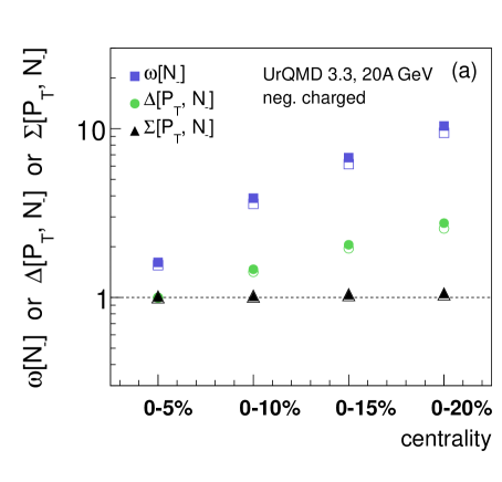
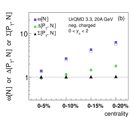
Refer to caption
Refer to caption
Figure 5: (Color online) The UrQMD results for the centrality dependence of ω[N]𝜔delimited-[]subscript𝑁\omega[N_{-}] (squares), Δ[PT,N]Δsubscript𝑃𝑇subscript𝑁\Delta[P_{T},N_{-}] (circles), and Σ[PT,N]Σsubscript𝑃𝑇subscript𝑁\Sigma[P_{T},N_{-}] (triangles) in Pb+Pb collisions at Elab=20subscript𝐸𝑙𝑎𝑏20E_{lab}=20A GeV. A centrality selection is done with a restriction on the impact parameter b𝑏b. (a): The full 4π4𝜋4\pi detector acceptance. (b): Only particles with center of mass rapidity in the interval 1<yπ<21subscript𝑦𝜋21<y_{\pi}<2 are accepted (pion mass was assumed for all particles). Open symbols correspond to the case when 10% of particles was randomly rejected.

We use the UrQMD simulations in Pb+Pb collisions at Elab=20subscript𝐸𝑙𝑎𝑏20E_{lab}=20 GeV per nucleon to study Δ[PT,N]Δsubscript𝑃𝑇subscript𝑁\Delta[P_{T},N_{-}] and Σ[PT,N]Σsubscript𝑃𝑇subscript𝑁\Sigma[P_{T},N_{-}]. With this example we illustrate effects of the centrality selection and limited detector acceptance and efficiency in A+A collisions. The results presented in Fig. 5 correspond to the centrality bins of 5%, 10%, 15%, and 20% most central Pb+Pb collisions. One observes very strong increase of ω[N]𝜔delimited-[]subscript𝑁\omega[N_{-}] with a width of the centrality bin. This reflects the fact that fluctuations of the number of nucleon participants affect strongly the fluctuations of final hadron multiplicities. Therefore, scaled variances as the fluctuation measures become almost useless for wide centrality bins. For these wide samples of collisions, the scaled variances do not describe physical properties of the system but reflect the system size fluctuations (see more details in Ref. HSD ). The strongly intensive measures Δ[PT,N]Δsubscript𝑃𝑇subscript𝑁\Delta[P_{T},N_{-}] and Σ[PT,N]Σsubscript𝑃𝑇subscript𝑁\Sigma[P_{T},N_{-}] look much more appropriate. These quantities are not sensitive to the trivial system size fluctuations. Their dependence on the size of the centrality bin is rather moderate (it is more pronounced for Δ[PT,N]Δsubscript𝑃𝑇subscript𝑁\Delta[P_{T},N_{-}]) and reflects changes in local physical properties for different centrality samples.

Another important aspect of today measurements of the e-by-e fluctuations in A+A collisions is a limited detector acceptance and/or efficiency. Particles may be lost due to the geometry of the detector (for example fixed target experiments typically cover only forward hemisphere) and we call it acceptance losses. On the other hand, even in this accepted kinematic region we still may have efficiency losses due to track reconstruction problems (including problems with ionization energy loss, dE/dx𝑑𝐸𝑑𝑥dE/dx, reconstruction).

The UrQMD results for negatively charged particles in Pb+Pb collisions at Elab=20subscript𝐸𝑙𝑎𝑏20E_{lab}=20A GeV for the full 4π𝜋\pi acceptance and for the particles accepted only in the center of mass rapidity interval 1<yπ<21subscript𝑦𝜋21<y_{\pi}<2 are shown in Fig. 5 (a) and (b), respectively (full symbols). From a comparison of the results for the full and limited detector acceptance one observes rather strong effects of acceptance losses for the scaled variance ω[N]𝜔delimited-[]subscript𝑁\omega[N_{-}]. The strongly intensive measures Δ[PT,N]Δsubscript𝑃𝑇subscript𝑁\Delta[P_{T},N_{-}] and Σ[PT,N]Σsubscript𝑃𝑇subscript𝑁\Sigma[P_{T},N_{-}] look again more appropriate. The effects of the limited acceptance are rather moderate for Δ[PT,N]Δsubscript𝑃𝑇subscript𝑁\Delta[P_{T},N_{-}] and almost absent for Σ[PT,N]Σsubscript𝑃𝑇subscript𝑁\Sigma[P_{T},N_{-}]. We also would like to stress that the acceptance dependence shown in Fig. 5 is the example only. In general, the measured magnitude of ω[N]𝜔delimited-[]𝑁\omega[N], Δ[PT,N]Δsubscript𝑃𝑇𝑁\Delta[P_{T},N] or Σ[PT,N]Σsubscript𝑃𝑇𝑁\Sigma[P_{T},N] depends on both the correlation(s) length(s) and the size of the acceptance region (when the kinematic acceptance is much smaller that the correlation range the effect will be washed out). Therefore, when comparing experimental results to models the experimental kinematic restrictions should be carefully taken into account.

Finally, the example of the effect of efficiency losses is shown by open symbols in Fig. 5. In this case from each event we randomly rejected 10% of particles. As seen, the effect of efficiency losses is small or even negligible (comparison of full and open symbols) for all presented fluctuation measures but, in general, it depends on the fraction of rejected particles.

VI Summary

In the present paper strongly intensive measures of the event-by-event fluctuations Δ[PT,N]Δsubscript𝑃𝑇𝑁\Delta[P_{T},N] and Σ[PT,N]Σsubscript𝑃𝑇𝑁\Sigma[P_{T},N] are studied. The recently proposed special normalization for these fluctuation measures are used, and it ensures that these measures are dimensionless and yields a common scale required for a quantitative comparison of fluctuations. Several phenomenological models are considered using the Monte Carlo simulations and analytical calculations. Our studies include different versions of the model of independent sources: with fixed number of sources, with the Poisson distribution of the number of sources, and with the Negative Binomial distribution. The quantities Δ[PT,N]Δsubscript𝑃𝑇𝑁\Delta[P_{T},N] and Σ[PT,N]Σsubscript𝑃𝑇𝑁\Sigma[P_{T},N] are found to be independent of the average number of sources and of its fluctuations. This reflects the strongly intensive properties of the ΔΔ\Delta and ΣΣ\Sigma measures, and is a main motivation of their using for the analysis of the event-by-event fluctuations in nucleus-nucleus collisions. The transverse momentum distribution of particles emitted from the source are assumed to be a thermal-like (Boltzmann) distribution over transverse mass. The average single-particle transverse momentum is then controlled by the inverse slope (temperature) parameter.

The system of sources with constant temperature appear to be equivalent to the model of independent sources, i.e. a relation Δ[PT,N]=Σ[PT,N]=1Δsubscript𝑃𝑇𝑁Σsubscript𝑃𝑇𝑁1\Delta[P_{T},N]=\Sigma[P_{T},N]=1 is obtained. For independent temperature fluctuations from source to source, one finds the correlations between transverse momenta of particles emitted from the same source. This leads to Δ[PT,N]=Σ[PT,N]=1+qSΔsubscript𝑃𝑇𝑁Σsubscript𝑃𝑇𝑁1subscript𝑞𝑆\Delta[P_{T},N]=\Sigma[P_{T},N]=1+q_{S}, where the value of qSsubscript𝑞𝑆q_{S} is positive and depends only on the parameters of a single source. If all sources have the same fluctuating temperature, the model of independent sources becomes no more applicable. One obtains Δ[PT,N]=Σ[PT,N]=1+QSΔsubscript𝑃𝑇𝑁Σsubscript𝑃𝑇𝑁1subscript𝑄𝑆\Delta[P_{T},N]=\Sigma[P_{T},N]=1+Q_{S}, where the value of QSsubscript𝑄𝑆Q_{S} increases linearly with the average number of sources NSdelimited-⟨⟩subscript𝑁𝑆\langle N_{S}\rangle and increases with σTsubscript𝜎𝑇\sigma_{T} which determines the size of temperature fluctuations.

A model which introduces a correlation between the temperature parameter and particle multiplicity is studied. In this case, the different values for the ΔΔ\Delta and ΣΣ\Sigma measures have been found: Δ[PT,N]=1+qδΔsubscript𝑃𝑇𝑁1subscript𝑞𝛿\Delta[P_{T},N]=1+q_{\delta} and Σ[PT,N]=1+qσΣsubscript𝑃𝑇𝑁1subscript𝑞𝜎\Sigma[P_{T},N]=1+q_{\sigma}. Analytical calculations under several simplifying assumptions give: qδ 4θsubscript𝑞𝛿4𝜃q_{\delta}\cong-\,4\theta and qσ2θ2subscript𝑞𝜎2superscript𝜃2q_{\sigma}\cong 2\theta^{2} , where the parameter θ𝜃\theta describes the correlations between TNsubscript𝑇𝑁T_{N} and N𝑁N according to (69) and is assumed to be small, |θ|1much-less-than𝜃1|\theta|\ll 1.

The UrQMD simulations for Pb+Pb collisions at the collision energy Elab=20subscript𝐸𝑙𝑎𝑏20E_{lab}=20 GeV per nucleon are done and analyzed. With this example we illustrate a role of the centrality selection and limited detector acceptance and efficiency in A+A collisions. We find that the strongly intensive quantities Δ[PT,N]Δsubscript𝑃𝑇𝑁\Delta[P_{T},N] and Σ[PT,N]Σsubscript𝑃𝑇𝑁\Sigma[P_{T},N] have an advantage over the standard fluctuation measures. In contrast to the scaled variance, Δ[PT,N]Δsubscript𝑃𝑇𝑁\Delta[P_{T},N] and Σ[PT,N]Σsubscript𝑃𝑇𝑁\Sigma[P_{T},N] demonstrate much weaker sensitivity to the width of the centrality bin and to the limited detector acceptance and efficiency.

In all considered model examples, Δ[PT,N]Δsubscript𝑃𝑇𝑁\Delta[P_{T},N] appears to be more sensitive to interparticle correlations than Σ[PT,N]Σsubscript𝑃𝑇𝑁\Sigma[P_{T},N]. This reveals itself as stronger deviations of Δ[PT,N]Δsubscript𝑃𝑇𝑁\Delta[P_{T},N] from the IPM results (14). Even for Δ[PT,N]=Σ[PT,N]Δsubscript𝑃𝑇𝑁Σsubscript𝑃𝑇𝑁\Delta[P_{T},N]=\Sigma[P_{T},N], in the MC simulations in Sec. III, a stronger sensitivity of Δ[PT,N]Δsubscript𝑃𝑇𝑁\Delta[P_{T},N] manifests as its larger statistical errors.

We hope that the results obtained in this paper will be helpful to elucidate the properties of Δ[PT,N]Δsubscript𝑃𝑇𝑁\Delta[P_{T},N] and Σ[PT,N]Σsubscript𝑃𝑇𝑁\Sigma[P_{T},N] measures.

Acknowledgements.
We would like to thank Marek Gaździcki, Laszlo Jenkovszky, and Stanislaw Mrówczyński for fruitful discussions and comments. We are indebted to the authors of the UrQMD model for the possibility to use their code in our analysis. The work of M.I.G. is supported by the State Agency of Science, Innovations and Informatization of Ukraine, contract F58/384-2013. The work of K.G. was supported by the the National Science Center, Poland grant DEC-2011/03/B/ST2/02617 and grant 2012/04/M/ST2/00816.

References

  • (1) M. Stephanov, K. Rajagopal, and E. V. Shuryak, Phys. Rev. D 60, 114028 (1999).
  • (2) F. Becattini, J. Manninen, and M. Gaździcki, Phys. Rev. C 73, 044905 (2006).
  • (3) M. Gaździcki [NA61/SHINE Collaboration], J. Phys. G 36, 064039 (2009).
  • (4) G. Odyniec [STAR Collaboration], J. Phys. G 35, 104164 (2008);
    A. Adare et al. [PHENIX Collaboration], Phys. Rev.  C 78, 044902 (2008).
  • (5) V. P. Konchakovski, M. I. Gorenstein, E. L. Bratkovskaya, and W. Greiner, J. Phys. G 37, 073101 (2010).
  • (6) M. I. Gorenstein and M. Gaździcki, Phys. Rev. C 84, 014904 (2011).
  • (7) K. Grebieszkow, Acta Phys. Polon. B 43, 1333 (2012).
  • (8) V. P. Konchakovski, V. V. Begun, M. I. Gorenstein, and E. L. Bratkovskaya, J. Phys. G 40, 045109 (2013).
  • (9) M. Gaździcki and S. Mrówczyński, Z. Phys. C 54, 127 (1992).
  • (10) H. Appelshauser et al. [NA49 Collaboration], Phys. Lett. B 459, 679 (1999).
  • (11) T. Anticic et al. [NA49 Collaboration], Phys. Rev. C 70, 034902 (2004).
  • (12) C. Alt et al. [NA49 Collaboration], Phys. Rev. C 70, 064903 (2004).
  • (13) T. Anticic et al. [NA49 Collaboration], Phys. Rev. C 79, 044904 (2009).
  • (14) D. Adamova et al. [CERES Collaboration], Nucl. Phys. A 727, 97 (2003).
  • (15) K. Adcox et al. [PHENIX Collaboration], Phys. Rev. C 66, 024901 (2002).
  • (16) M. R. Atayan et al. [EHS/NA22 Collaboration], Phys. Rev. Lett.  89, 121802 (2002).
  • (17) M. Bleicher, M. Belkacem, C. Ernst, H. Weber, L. Gerland, C. Spieles, S. A. Bass and H. Stoecker et al., Phys. Lett. B 435, 9 (1998).
  • (18) S. Mrówczyński, Phys. Lett. B 439, 6 (1998).
  • (19) F. Liu, A. Tai, M. Gazdzicki and R. Stock, Eur. Phys. J. C 8, 649 (1999).
  • (20) S. Mrówczyński, Phys. Lett. B 459, 13 (1999).
  • (21) S. Mrówczyński, Phys. Lett. B 465, 8 (1999).
  • (22) S. Mrówczyński, Acta Phys. Polon. B 31, 2065 (2000).
  • (23) O. V. Utyuzh, G. Wilk and Z. Wlodarczyk, Phys. Rev. C 64, 027901 (2001).
  • (24) R. Korus and S. Mrówczyński, Phys. Rev. C 64, 054906 (2001).
  • (25) R. Korus, S. Mrówczyński, M. Rybczynski and Z. Wlodarczyk, Phys. Rev. C 64, 054908 (2001).
  • (26) J. Zaranek, Phys. Rev. C 66, 024905 (2002).
  • (27) O. Pruneau, S. Gavin and S. Voloshin, Phys. Rev. C 66, 044904 (2002).
  • (28) S. Mrówczyński and E. V. Shuryak, Acta Phys. Polon. B 34, 4241 (2003).
  • (29) S. Mrówczyński, M. Rybczynski, and Z. Włodarczyk, Phys. Rev. C 70, 054906 (2004).
  • (30) Q. H. Zhang, L. Huo, W. N. Zhang, L. Huo and W. N. Zhang, Phys. Rev. C 72, 047901 (2005).
  • (31) K. Grebieszkow, Phys. Rev. C 76, 064908 (2007).
  • (32) W. M. Alberico and A. Lavagno, Eur. Phys. J. A 40, 313 (2009).
  • (33) M. Gaździcki, M. I. Gorenstein, and M. Mackowiak-Pawlowska, Phys. Rev. C 88, 024907 (2013).
  • (34) M. I. Gorenstein and M. Rybczynski, arXiv:1308.0752 [nucl-th], Phys. Lett. B, in print.
  • (35) T. Czopowicz [NA61 Collaboration], ”Results from NA61/SHINE ion program”, slides from 16th Lomonosov Conference on Elementary Particle Physics, Moscow, August 2013; http://www.icas.ru/english/LomCon/16lomcon/16lomcon__\textunderscoreprogramme.htm ;
    P. Seyboth [NA49 and NA61 Collaborations], ”Recent results from the search for the critical point of strongly interacting matter at the CERN SPS”, slides from XLIII International Symposium on Multiparticle Dynamics (ISMD), Chicago, September 2013, https://indico.hep.anl.gov/indico/conferenceDisplay.py?confId=0 .
  • (36) A. Bialas, M. Bleszynski, and W. Czyz, Nucl. Phys. B 111, 461 (1976).
  • (37) V. V. Begun, M. Gazdzicki, and M. I. Gorenstein, Phys. Rev. C 78, 024904 (2008).
  • (38) G. Wilk and Z. Włodarczyk, Phys. Rev. C 79, 054903 (2009); J. Phys. G 38, 065101 (2011); Eur. Phys. J. A 48, 161 (2012).
  • (39) S. A. Bass et al., Prog. Part. Nucl. Phys. 41, 255 (1998);
    M. Bleicher et al., J. Phys. G 25, 1859 (1999).