Visualizing Basins of Attraction
for Different Minimization Algorithms

Abstract

We report a study of the basins of attraction for potential energy minima defined by different minimisation algorithms for an atomic system. We find that whereas some minimisation algorithms produce compact basins, others produce basins with complex boundaries or basins consisting of disconnected parts. Such basins deviate from the ‘correct’ basin of attraction defined by steepest-descent pathways, and the differences can be controlled to some extent by adjustment of the maximum step size. The choice of the most convenient minimisation algorithm depends on the problem in hand. We show that while L-BFGS is the fastest minimiser, the FIRE algorithm is also quite fast, and can lead to less fragmented basins of attraction.

+44 (0)1223 336530

Keywords: optimisation, quench, energy landscape, meta-basin analysis, inherent structure, transition state.

1 Introduction

Optimisation problems are ubiquitous in the physical sciences and beyond. In the simplest case optimisation refers to the search for the minimum or maximum values of an objective function. Global optimisation involves searching for the highest maximum or lowest minimum in a certain domain. In contrast, local optimisation procedures identify the first minimum or maximum that is found by a given algorithm when starting from an arbitrary point in parameter space.

In the study of energy landscapes, the properties of stationary points and the connections between them are of central importance.¹ These stationary points represent key features of the landscape. In chemical reactions, saddle points are geometric transition states ² along the reaction coordinate. Glassy systems are trapped in metastable states that correspond to relatively small numbers of connected local minima ^{3, 4, 5} and, similarly, jammed states can also be viewed as local potential energy minima. In protein folding the native state corresponds to the global free energy minimum and the free energy landscape often involves funnelling characteristics.⁶ The study of these minima and the pathways connecting them can be carried out using geometry optimisation techniques,^{1, 7} and local minimisation is the focus of the current contribution.

When faced with the task of numerically optimising a smooth function there are many algorithms from which to choose. Which algorithm is best suited for the purpose depends on factors such as speed, memory usage and ease of implementation. All algorithms follow a general procedure starting with the user supplying an initial point, which can be an informed guess or an arbitrary point in parameter space. The algorithm generates a sequence of iterates that terminates when a solution is found within a predefined accuracy, such as when the gradient is near zero, or when the value of the function stops changing. Recent work has shown how convergence criteria can be chosen according to a certification procedure.⁸ Different algorithms have different ways of proceeding from one iteration to the next. The formulations we consider involve the value of the function that is being optimised, its derivatives, and the results of previous iterations.

In general, two different algorithms can converge to different minima starting from the same initial conditions. We are interested in identifying the configuration space that leads to a particular minimum as a function of the optimisation algorithm. This connection is important for applications such as calculation of thermodynamic properties using the superposition approach, where the global partition function is written as a sum over contributions of local minima.^{9, 10, 11} In this context, the steepest-descent algorithm occupies a unique position, since it defines basins of attraction¹² for local minima that cannot interpenetrate. This result follows because steepest-descent paths are defined using a linear first-order differential equation, for which the uniqueness theorem applies.¹³ However, steepest-descent minimisation is very inefficient compared to more sophisticated algorithms, which are normally preferable. The latter methods generally employ non-linear equations to determine the steps, and the corresponding basins of attraction can exhibit complex boundaries.^{14, 15} In other words, when defined by steepest-descent, the basin of attraction has a deterministic boundary. In contrast, the basins for other algorithms can exhibit re-entrant, interpenetrating boundaries, as noted in previous work.^{14, 15} For applications such as basin-hopping global optimisation^{16, 17} this structure is probably unimportant. However, the simplicity of the boundaries associated with steepest-descent paths is relevant if we are interested in partitioning the configuration space, for example, when measuring the size of basins of attraction. ¹⁸ In the present work, we regard the basins of attraction defined by steepest descent as a reference to which other methods will be compared. The purpose of this paper is to make these comparisons rigorously and to provide criteria for choosing the most appropriate and convenient minimisation algorithm for a given problem.

2 Methods

The minimisation algorithms considered here are steepest-descent, L-BFGS, FIRE, conjugate gradient, and BFGS (for a detailed description of different minimisation techniques see reference¹⁹). The L-BFGS algorithm is tested using two different methods to determine the length of the steps. In the first approach, a line search routine is used to choose the step size. In the second approach, the step size guess of the L-BFGS algorithm is accepted subject to a maximum step size and the condition that the energy does not rise. This is the default procedure in the global optimisation program GMIN²⁰ and the OPTIM program for locating transition states and analysing pathways.²¹ We have only compared gradient-based minimisers in the present work, because they represent the most efficient class of algorithms.

Steepest-descent, sometimes referred to as gradient descent, uses the gradient as the search direction (this is the steepest direction). The step size can be chosen using a line search routine. In this paper, a fixed step size ($\Delta=0.005$ in reduced units) is used for all of the steepest-descent calculations. It is worth noting that the definition of basins of attraction in the Introduction section applies to steepest-descent minimisation in the limit of infinitesimal step size.

BFGS, named after its creators Broyden,²² Fletcher,²³ Goldfarb,²⁴ and Shanno,²⁵ is a quasi-Newtonian optimisation method, which uses an approximate Hessian to determine the search direction. The approximate Hessian is built up iteratively from the history of steps and gradient evaluations. The implementation used in this paper is from SciPy²⁶ and uses a line search to determine a step size. The line search used is the Minpack2 method DCSRCH,²⁷ which attempts to find a step size that satisfies the Wolfe conditions. The maximum step size is fixed to be $50$ times the initial guess returned by the BFGS algorithm.

L-BFGS is a limited memory version of the BFGS algorithm described above and was designed for large-scale problems, where storing the Hessian would be impractical. Rather than saving the full approximate Hessian in memory it only stores a history of $M$ previous values of the function and its gradient with which it computes an approximation to the inverse diagonal components of the Hessian.²⁸ For a system with $N$ variables, ${\cal O}(N^{2})$ memory and operations are needed when using BFGS, while L-BFGS scales as ${\cal O}(MN)$, which is significantly smaller if $M\ll N$, and is linear in $N$. Two versions of L-BFGS were used in this paper. The first is from the SciPy²⁶ optimisation library ”L-BFGS-B”.^{29, 30, 31} This routine uses the same DCSRCH line search as the BFGS implementation, but with slightly different input parameters. For example, the maximum step size is adaptively updated. The second L-BFGS implementation is included in the GMIN²⁰ and OPTIM²¹ software packages and adapted from Liu and Nocedal.²⁸ In this version there is no line search. The step size returned by the L-BFGS algorithm is accepted subject to a maximum step size constraint and the condition that the energy does not rise. In both of these versions, the diagonal components of the inverse Hessian are initially set to unity.

The fast inertial relaxation engine, known as FIRE, is a minimisation algorithm based on ideas from molecular dynamics, with an extra velocity term and adaptive time step.³² Stated simply, the system state slides down the potential energy surface gathering “momentum” until the direction of the gradient changes, at which point it stops, resets, and resumes sliding.

The conjugate gradient method uses information about previous values of the gradient to determine a conjugate search direction.³³ It only stores the previous search direction. The implementation considered here is from SciPy,²⁶ and the step size is determined using same line search as the BFGS routine.

In order to test the accuracy of the minimisers, we use a three-particle system in which the inter-particle interactions are given by a Lennard-Jones potential plus a three-body Axilrod–Teller term:^{34, 35}

$$V = 4\varepsilon\sum_{i<j}\left[\left(\frac{\sigma}{r_{ij}}\right)^{12}-\left(\frac{\sigma}{r_{ij}}\right)^{6}\right]+$$

$$\qquad Z\sum_{i<j<k}\left[\frac{1+3\cos\theta_{1}\cos\theta_{2}\cos\theta_{3}}{(r_{ij}r_{ik}r_{jk})^{3}}\right],$$

Here $\theta_{1}$, $\theta_{2}$ and $\theta_{3}$ are the internal angles of the triangle formed by particles $i$, $j$, $k$; $r_{ij}$ is the distance between particles $i$ and $j$; and $Z$ is the strength of the three-body term. We chose this three-particle system because, for $Z>0$, it has four local minima. It was important for us to choose a small system with only a few degrees of freedom in order to visualise the basins of attraction in two dimensions. In one of the minima, the atoms are arranged in an equilateral triangle, with point group $D_{3h}$. The other three linear minima have $D_{\infty h}$ symmetry and are related by permutations of the atoms. We use reduced units with one parameter, as in previous work:^{36, 37, 14, 15}

$$Z^{*}=\frac{Z\sigma^{9}}{\varepsilon}.$$ (2)

Without loss of generality, we define the axes such that the three particles are in the $xy$ plane with one particle at the origin, another along the $x$ axis, and the third in the upper half plane. Now only the three internal coordinates $r_{ij}$ are needed to describe the system. A projection onto the page was chosen to visualise the basins of attraction in such a way that the basins of the four minima are present in the plane.^{14, 15} In internal coordinates, the projection plane is chosen to be perpendicular to the vector $\vec{n}=(1,1,1)$ at a distance $\sqrt{3}\alpha$ from the origin. Points in the plane have the property $r_{12}+r_{23}+r_{13}=3\alpha$. We can define an arbitrary vector $\vec{v}=(0,0,1)$ so that the plane is spanned by the unit vectors

$$\hat{x}_{2}=\frac{\vec{n}\times\vec{v}}{|\vec{n}\times\vec{v}|},\qquad\hat{x}_{1}=\frac{\vec{n}\times\vec{x}_{2}}{|\vec{n}\times\vec{x}_{2}|}.$$ (3)

The projection of an arbitrary vector $\vec{a}=(r_{12},r_{23},r_{13})$ onto the plane is $\vec{a}_{p}=(\vec{a}\cdot\hat{x}_{1},\vec{a}\cdot\hat{x}_{2})$. The equilateral triangle minimum is at the origin in terms of the projected coordinates $x_{1}$ and $x_{2}$, as shown in 1. For more details regarding the projection see references ^{14, 15}.

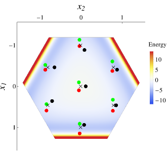
Figure 1: Projected plane in its own coordinate system. Points on this plane were used as the initial configurations for the minimisations. Examples of starting configurations are shown for several points marked by “$\times$”. The plot is coloured by the energy of the starting configuration.

The following results were produced using the projection described above with $\alpha=\sqrt{3}R_{e}$, where $R_{e}=2^{1/6}\sigma$ is the Lennard-Jones equilibrium separation, and $Z^{*}=2$. For this choice there is a linear minimum with energy $-2.219\,\varepsilon$ in addition to the equilateral triangle with energy $-2.185\,\varepsilon$. There are three distinct permutational isomers of the linear minimum, since any of the three atoms can reside in the central position. A $700\times 700$ grid of initial points was taken with $x_{1}$ and $x_{2}$ between $-\alpha$ and $\alpha$. All of the minimisations were terminated when the root mean square (RMS) gradient was smaller than $10^{-3}$ reduced units. Under some conditions, such geometry optimisations could appear to converge to a saddle point,³⁸ so the geometries were also checked, as well as the RMS gradient. As in previous work,^{14, 15} each pixel in the resulting plots corresponds to a different initial configuration and is coloured according to the minimum that is found after optimisation.

The efficiency of each algorithm was also tested. Here we were not constrained to small systems by the need for visualisation, so we chose a more interesting system size, namely 38 Lennard-Jones atoms. We measured the average number of function calls needed to get to the nearest local minimum from 1,000 random starting configurations. The number of function calls is a fairer test than wall clock time because for most real word calculations computing the energy and gradient will be the time bottleneck and it avoids measuring differences in implementation efficiency. The results are reported in 2.

3 Results and Discussion

2 shows the colour scheme used to identify the results of local minimisation in the subsequent figures. Forbidden geometry refers to the points in the plane that correspond to initial geometries that do not satisfy the triangle inequality or have excessively high energy. Failed quench means that the quenched coordinates are not close enough (according to a certain tolerance) to the equilateral triangle or linear configurations, that is, the algorithm failed to reach a minimum.³⁸

Steepest-descent, $\Delta=0.005$

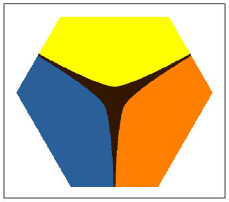
Figure 2: The lower panel shows the same $(x_{1},x_{2})$ plane as 1, which defines the starting configuration of the three particles that interact via the Lennard-Jones potential plus a three-body Axilrod-Teller term, as described in the Methods Section. The plane is coloured according to the final configuration after a steepest-descent minimisation. The colour coding is displayed in the upper panel. Black corresponds to the atoms in the $D_{3h}$ triangle configuration, while blue, orange, and yellow correspond to the three possible linear configurations. A failed quench means that the final coordinates are not close enough (according to a certain tolerance) to the equilateral triangle or linear configurations. $\Delta$ is the maximum step size. This figure, corresponding to the steepest-descent results, will serve as our reference for comparing the other minimisers.

The figures that follow show the basins of attraction of the four minima described above determined using the different minimisation techniques and parameters, as described in the Methods section. As expected, steepest-descent is the slowest (see 1), most robust minimiser, and it produces well-defined basin boundaries (2). This result holds as long as the step size is kept relatively small. Smaller step sizes are always more robust when using steepest-descent. The usual definition for the basin of attraction in the context of energy landscapes is the set of points in configuration space that converge to a certain minimum for a steepest-descent quench.^{12, 1} Hence this approach produces a useful reference against which to compare the other algorithms.

L-BFGS is the fastest algorithm tested here (see 2), although the basin boundaries are not always well defined (see 3 and 6). In the case of L-BFGS without line search we can see that reducing the step size does not necessarily improve the definition of the basin boundaries. In this case, the resolution of the basin boundaries improves with increasing maximum step size until it reaches an optimum length, beyond which the resolution decreases. This effect is clearly visible in 1 and 3. Removing the line search does not improve the resolution of the boundaries, but it does reduce the number of failed quenches. We tested the effect of changing the parameter $M$, the number of previous values of the function and gradient used to build the approximate Hessian. Increasing $M$ between 1 and 10 makes the resolution of the basins worse (see 3) but produces faster convergence (see 1). This result arises due to the fact that increasing $M$ increases the degree of non-linearity of the algorithm.

L-BFGS, $M=1$, $\Delta=0.05$ L-BFGS, $M=1$, $\Delta=0.1$ L-BFGS, $M=1$, $\Delta=0.2$
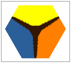
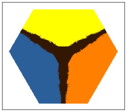
L-BFGS, $M=4$, $\Delta=0.05$ L-BFGS, $M=4$, $\Delta=0.1$ L-BFGS, $M=4$, $\Delta=0.2$
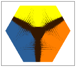
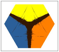
L-BFGS, $M=10$, $\Delta=0.05$ L-BFGS, $M=10$, $\Delta=0.1$ L-BFGS, $M=10$, $\Delta=0.2$

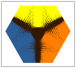
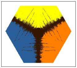
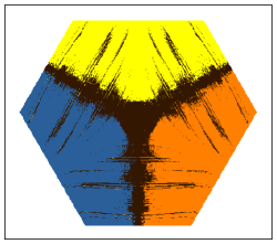
Figure 3: Results for the L-BFGS algorithm for different values of $M$ (the number of previous steps used to construct the next step) and the maximum step size $\Delta$. See 2 for a detailed explanation of the figure.

Several values of the maximum step size for FIRE were tested. For a small value of the step size the boundaries of the basins of attraction are well defined and similar to the results for steepest-descent. The method only ends up in the wrong basin when starting from points that lie very close to the boundaries between two basins (4, top left). Using a larger value of the step size leads to many artifacts and failed quenches, which are evident in the bottom half of 4.

FIRE, $\Delta=0.1$                                   FIRE, $\Delta=0.25$

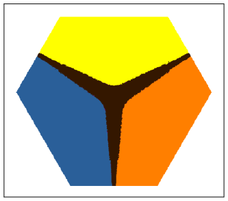
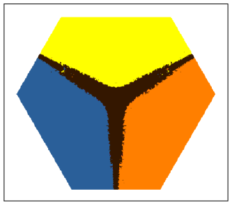
FIRE, $\Delta=0.5$

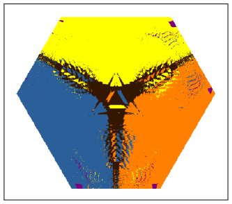
Figure 4: Results for the FIRE algorithm for several values of the maximum step size $\Delta$. The bottom right panel is a magnification of a portion of the bottom left image. See 2 for a detailed explanation of the figure.

Some other popular algorithms were also tested, namely, conjugate gradient (5) and BFGS (6). The SciPy implementation of these methods uses the same line search routine to determine the step size at each iteration, and both of them produce similar ill-defined basin boundaries. In both cases, the boundary artifacts are caused by the line search returning a step size that is large enough to move into a different basin. Furthermore, the failed quenches at the edges are due to step sizes sufficiently large that particles end up so far apart that the gradient is small enough to satisfy the termination condition. The line search algorithm is not entirely responsible for the imprecise basin boundaries. The initial guess for the step size passed to the line search by the conjugate gradient and BFGS algorithms is often large enough to step to the next basin by itself. To check this effect, we have also tested this line search routine with the L-BFGS algorithm. The results (not shown for brevity) produce quite reasonable basin boundaries with most of the above artifacts absent. An interesting question is why the L-BFGS algorithm produces an accurate guess for the step size while BFGS tends to overestimate the step size. The answer, most likely, is that the initial Hessian in L-BFGS is scaled,²⁸ while in BFGS it is fixed to unity.

We wanted to test the effect of maximum step size on the conjugate gradient and BFGS algorithms; however the SciPy routines do not accept parameters for adjusting the maximum step size. We were able to introduce this adjustment by modifying the source code of the line search routine used in each case. With these modifications and a maximum step size of $0.1$, the conjugate gradient routine produced reasonably accurate basin boundaries. The penalty for this improved precision was roughly $50\%$ more function evaluations. We were not able to obtain significant improvements for the BFGS routine.

Conjugate gradient, with line search (SciPy)

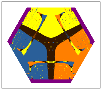
Figure 5: Results for the conjugate gradient algorithm with line search (SciPy implementation) are shown in the left panel. The right panel shows a magnification of the left panel. See 2 for a detailed explanation of the figure.

L-BFGS, with line search (SciPy)               BFGS, with line search (SciPy)

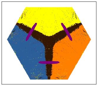
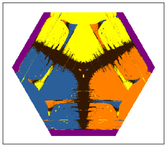
Figure 6: Results for L-BFGS and BFGS with line search (SciPy implementations). See 2 for a detailed explanation of the figure.

The basins of attraction determined by some of the methods mentioned above (in particular FIRE with a large step size, conjugate gradient and BFGS) display complex structures, as shown in 4 (bottom right) and 5 (right). Here we can see that the basin boundaries still have structure, even as the length scale is reduced. As noted in previous work, the structure may be fractal, ^{39, 14, 15} although this possibility was not investigated in detail.

Table 1: Table showing the quantitative analysis of the basins of attraction defined by different minimisers for the three-body system. The third column, Err, is the percentage of starting configurations that minimised to a different minimum compared to the steepest-descent method. $\Delta$ is the maximum step size and $M$ is the length of the history used by L-BFGS, as defined in the Methods section.

Algorithm	Parameters	Err (%)
L-BFGS	$M=1$, $\phantom{0}\Delta=0.05$	6.41
(without LS)	$M=1$, $\phantom{0}\Delta=0.1$	6.46
	$M=1$, $\phantom{0}\Delta=0.2$	7.16
	$M=4$, $\phantom{0}\Delta=0.05$	14.75
	$M=4$, $\phantom{0}\Delta=0.1$	10.84
	$M=4$, $\phantom{0}\Delta=0.2$	10.13
	$M=10$, $\Delta=0.05$	16.78
	$M=10$, $\Delta=0.1$	12.72
	$M=10$, $\Delta=0.2$	14.81
L-BFGS
(SciPy, with LS)	$M=10$	12.79
FIRE	$\Delta=0.1$	3.68
	$\Delta=0.25$	4.53
	$\Delta=0.5$	11.23
BFGS
(SciPy, with LS)		23.45
CG
(SciPy, with LS)		22.93
Steepest-Descent	$\Delta=0.001$	0.00

We have quantified the difference between the outcomes of the basin mapping for different minimisers by counting the number of starting structures for which we find a basin different from the one obtained using steepest-descent, as shown in 1. This difference corresponds to the number of different structures (from a total of 170,607 valid starting structures) when comparing the minimum produced by the corresponding algorithm with the minimum produced by steepest-descent (2).

Table 2: Benchmarks for the algorithms tested in this paper in terms of the average number of function calls $\langle$FCs$\rangle$ needed to minimise a 38-particle Lennard-Jones system from a random configuration. The stopping condition is that the maximum force on any atom is less than 0.01 in reduced units.

Algorithm	Parameters	$\langle$FCs$\rangle$
L-BFGS	$M=1$, $\phantom{0}\Delta=0.1$	273
(without LS)	$M=4$, $\phantom{0}\Delta=0.05$	369
	$M=4$, $\phantom{0}\Delta=0.1$	241
	$M=4$, $\phantom{0}\Delta=0.2$	225
	$M=10$, $\Delta=0.1$	228
	$M=20$, $\Delta=0.1$	216
L-BFGS
(SciPy, with LS)	$M=10$	215
FIRE	$\Delta=0.1$	822
	$\Delta=0.5$	3,185
BFGS
(SciPy, with LS)		1,233
CG
(SciPy, with LS)		837
Steepest-Descent	$\Delta=0.001$	31,672

2 reports the performance of the algorithms tested here in terms of the average number of times that the energy and the force were evaluated $\langle$FCs$\rangle$. The average is taken over a sample of 1,000 random initial states for a 38-particle Lennard-Jones cluster. The number of evaluations ultimately determines the time it takes to find a minimum, as this is generally the most time consuming part of any minimisation algorithm. We can see that L-BFGS is the fastest and FIRE is about three to four times slower, while steepest-descent is orders of magnitude slower, as expected.

4 Conclusions

In this paper, we have mapped the basins of attraction of a simple system onto a plane to compare a number of minimisation algorithms. We are able to compare the different approaches both visually and quantitatively, building upon previous work, where the focus was mainly on transition state searches.^{14, 15} Some of the more complex algorithms (CG, BFGS, L-BFGS and FIRE) depending on the choice of parameters produce basins that consist of disconnected parts. Such basins deviate from the “correct” basin of attraction defined by steepest-descent pathways, especially at the basin boundaries, where complex interpenetrating patterns can appear. These patterns generally do not disappear as the length scale is reduced, as can be seen in 4 and 5, making the basins ill-defined. In particular, we have found that overestimates for the step size are primarily responsible for the complex basin boundaries. Imposing a maximum step size can mitigate this problem for some algorithms, at the cost of slightly higher computational effort and an additional, system dependent, parameter. An appropriate value for the maximum step size can be chosen based on length scales in the system: for atomic systems, a good choice is about one tenth of the inter-atomic pair equilibrium distance.

In conclusion, if assignment of a starting configuration to the basin of attraction defined by steepest-descent is important, then FIRE may be the most convenient algorithm, due to its speed and precision, provided that an acceptable maximum step size is chosen. If finding a minimum quickly is more important, then L-BFGS is clearly the best choice.

The authors thank Dr Victor Rühle for many useful discussions and acknowledge funding from EPSRC Programme Grants EP/I001352/1 and EP/I00844/1, ERC Advanced Grants RG59508 and 227758, Marie Curie Grant 275544, Wolfson Merit Award 502011.K701/JE and Becas Chile CONICYT.

References

- Wales 2003 Wales, D. J. Energy Landscapes: With Applications to Clusters, Biomolecules and Glasses; Cambridge University Press: Cambridge, U.K., 2003
- Murrell and Laidler 1968 Murrell, J. N.; Laidler, K. J. Trans. Faraday. Soc. 1968, 64, 371–377
- Kirkpatrick et al. 1989 Kirkpatrick, T. R.; Thirumalai, D.; Wolynes, P. G. Phys. Rev. A 1989, 40, 1045
- Doliwa and Heuer 2003 Doliwa, B.; Heuer, A. Phys. Rev. E 2003, 67, 031506
- de Souza and Wales 2008 de Souza, V. K.; Wales, D. J. J. Chem. Phys. 2008, 129, 164507
- Wolynes et al. 1995 Wolynes, P.; Onuchic, J.; Thirumalai, D. Science 1995, 267, 1619–1620
- Wales and Bogdan 2006 Wales, D. J.; Bogdan, T. V. J. Phys. Chem. B 2006, 110, 20765–20776
- Mehta et al. 2013 Mehta, D.; Hauenstein, J. D.; Wales, D. J. J. Chem. Phys. Commun, 2013, 000, 000000
- Wales 1993 Wales, D. J. Mol. Phys. 1993, 78, 151–171
- Doye and Wales 1995 Doye, J. P. K.; Wales, D. J. J. Chem. Phys. 1995, 102, 9673–9688
- Strodel and Wales 2008 Strodel, B.; Wales, D. J. Chem. Phys. Lett. 2008, 466, 105–115
- Mezey 1981 Mezey, P. G. Theo. Chim. Acta 1981, 58, 309
- Pechukas 1976 Pechukas, P. J. Chem. Phys. 1976, 64, 1516
- Wales 1992 Wales, D. J. J. Chem. Soc., Faraday Trans. 1992, 88, 653
- Wales 1993 Wales, D. J. J. Chem. Soc., Faraday Trans. 1993, 89, 1305
- Wales and Doye 1997 Wales, D. J.; Doye, J. P. K. J. Phys. Chem. A 1997, 101, 5111–5116
- Li and Scheraga 1987 Li, Z.; Scheraga, H. A. Proc. Natl. Acad. Sci. U.S.A. 1987, 84, 6611
- Xu et al. 2011 Xu, N.; Frenkel, D.; Liu, A. J. Phys. Rev. Lett. 2011, 106, 245502
- Nocedal and Wright 1999 Nocedal, J.; Wright, S. Numerical Optimization; Springer Science+Business Media: New York, NY, U.S.A., 1999
- 20 Wales, D. J. GMIN: A Program for Finding Global Minima and Calculating Thermodynamic Properties from Basin-sampling. \urlhttp://www-wales.ch.cam.ac.uk/GMIN/
- 21 Wales, D. J. OPTIM: A Program for Optimising Geometries and Calculating Pathways
- Broyden 1970 Broyden, C. G. IMA J. Appl. Math. 1970, 6, 76–90
- Fletcher 1970 Fletcher, R. Comput. J. 1970, 13, 317–322
- Goldfarb 1970 Goldfarb, D. Math. Comp. 1970, 24, 23–26
- Shanno 1970 Shanno, D. F. Math. Comp. 1970, 24, 647–656
- Jones et al. 2001– Jones, E.; Oliphant, T.; Peterson, P. SciPy: Open source Scientific Tools for Python, 2001–. \urlhttp://www.scipy.org/
- More and Thuente 1994 More, J. J.; Thuente, D. J. Acm T. Math. Software 1994, 20, 286–307
- Liu and Nocedal 1989 Liu, D. C.; Nocedal, J. Math. Program. 1989, 45, 503–528
- Zhu et al. 1997 Zhu, C.; Byrd, R. H.; Lu, P.; Nocedal, J. ACM Trans. Math. Software 1997, 23, 550–560
- Byrd et al. 1995 Byrd, R.; Lu, P.; Nocedal, J.; Zhu, C. SIAM J. Sci. Comput. 1995, 16, 1190–1208
- Morales and Nocedal 2011 Morales, J. L.; Nocedal, J. ACM Trans. Math. Software 2011, 38, 7:1–7:4
- Bitzek et al. 2006 Bitzek, E.; Koskinen, P.; Gähler, F.; Moseler, M.; Gumbsch, P. Phys. Rev. Lett. 2006, 97, 170201
- Hestenes and Stiefel 1952 Hestenes, M. R.; Stiefel, E. J. Res. Nat. Bur. Stand. 1952, 49, 409–436
- Lennard-Jones 1924 Lennard-Jones, J. E. Proc. R. Soc. A 1924, 106, 463–477
- Axilrod and Teller 1943 Axilrod, B. M.; Teller, E. J. Chem. Phys. 1943, 11, 299–300
- Wales 1990 Wales, D. J. J. Chem. Soc., Faraday Trans. 1990, 86, 3505–3517
- Doye and Wales 1992 Doye, J. P. K.; Wales, D. J. J. Chem. Soc., Faraday Trans. 1992, 88, 3295–3304
- Uppenbrink and Wales 1992 Uppenbrink, J.; Wales, D. J. Chem. Phys. Lett. 1992, 190, 447–452
- Grebogi et al. 1987 Grebogi, C.; Ott, E.; Yorke, J. A. Science 1987, 238, 632–638