Linear Regression from Strategic Data Sources

Abstract

Linear regression is a fundamental building block of statistical data analysis. It amounts to estimating the parameters of a linear model that maps input features to corresponding outputs. In the classical setting where the precision of each data point is fixed, the famous Aitken/Gauss-Markov theorem in statistics states that generalized least squares (GLS) is a so-called “Best Linear Unbiased Estimator” (BLUE). In modern data science, however, one often faces strategic data sources, namely, individuals who incur a cost for providing high-precision data. For instance, this is the case for personal data, whose revelation may affect an individual’s privacy—which can be modeled as a cost—or in applications such as recommender systems, where producing an accurate estimate entails effort.

In this paper, we study a setting in which features are public but individuals choose the precision of the outputs they reveal to an analyst. We assume that the analyst performs linear regression on this dataset, and individuals benefit from the outcome of this estimation. We model this scenario as a game where individuals minimize a cost comprising two components: (a) an (agent-specific) disclosure cost for providing high-precision data; and (b) a (global) estimation cost representing the inaccuracy in the linear model estimate. In this game, the linear model estimate is a public good that benefits all individuals. We establish that this game has a unique non-trivial Nash equilibrium. We study the efficiency of this equilibrium and we prove tight bounds on the price of stability for a large class of disclosure and estimation costs. Finally, we study the estimator accuracy achieved at equilibrium. We show that, in general, Aitken’s theorem does not hold under strategic data sources, though it does hold if individuals have identical disclosure costs (up to a multiplicative factor). When individuals have non-identical costs, we derive a bound on the improvement of the equilibrium estimation cost that can be achieved by deviating from GLS, under mild assumptions on the disclosure cost functions.

Keywords: Linear regression, Aitken theorem, Gauss-Markov theorem, strategic data sources, potential game, price of stability

1 Introduction

The statistical analysis of data is a cornerstone of many scientific disciplines. The core problem of estimating the parameters of a model is classic, and is well understood in the standard setting in which any noise or distortions present in the data are exogenous. Naturally, the quality of the data, as captured by such noise or distortions, is key to an estimator’s accuracy. In many instances, however, obtaining high quality data may be associated with a cost incurred by the data source. For example, this is the case when the data is of a personal nature and provided by privacy-conscious individuals. The quality of the data provided in this case can come at a cost of a violation of privacy [24, 33, 15]. The desire for privacy incentivizes individuals to obfuscate their private information, or, in the extreme, altogether refrain from any disclosure. An additional setting in which high-quality data may come at a cost is when the data quality depends on effort exerted [8, 48], i.e., improved quality is the result of increased effort expended by the data source. This setting naturally arises in, e.g., open collaboration projects, such as wikipedia, but also in online recommender systems, where individuals need to exert effort (complete surveys, click “like” buttons, etc.) to disclose their preferences. Just as in the privacy case, a data source may choose to not exert the effort required to produce high-quality, low-noise responses or, in the extreme, altogether refrain from reporting anything meaningful.

In this setting, where providing high-quality data comes at a cost, it makes sense to consider strategic behavior among data sources. In particular, one should ask: why would strategic data sources provide any data at all? The existing literature focuses either on the case where individuals receive a monetary compensation to provide data [24, 15, 8, 35, 48, 1], or on the case where individuals care about the quality of the estimation but only w.r.t. predictions over their own features [18, 11, 41]. We consider another possibility, namely, that globally successful data analysis may also provide a utility to the individuals from which the data is collected. This is evident in medical studies: an experiment may lead to the discovery of a treatment for a disease, from which an experiment subject may benefit. In the case of recommender systems, users may indirectly benefit from overall service improvements, as data disclosed may lead to, e.g., improved product recommendations or better-targeted advertising. Similarly, open collaboration projects, by their nature, implicitly assume a common underlying utility, linked to the success of the collaboration. If such benefits outweigh associated privacy or effort costs, individuals may consent to the collection and analysis of high-quality data, e.g., by participating in a clinical trial, completing a survey, or disclosing their preferences in a recommender service.

In this paper, we approach the above issues through a non-cooperative game, focusing on the basic statistical analysis task of linear regression. We consider the following formal setting. A set of individuals $i\in\{1,\ldots,n\}$ participate in an experiment in which they are asked to provide data to an analyst. Each individual $i$ is associated with a feature vector $\boldsymbol{x}_{i}\in\mathbb{R}^{d}$, capturing public information such as age, gender, etc., and possesses a private variable $y_{i}\in\mathbb{R}$—e.g., the true answer to a survey, the outcome of a medical test, or how much they like a product. The analyst wishes to perform linear regression over the data, i.e., compute a vector $\boldsymbol{\beta}\in\mathbb{R}^{d}$ such that:

$$y_{i}\approx\boldsymbol{\beta}^{T}\boldsymbol{x}_{i},\qquad\text{for all }i\in\{1,\ldots,n\}.$$

We assume that individuals benefit from the correct estimation of $\boldsymbol{\beta}$: for example, if the analyst learns $\boldsymbol{\beta}$, an individual may benefit due to, e.g., better medical treatment, improved recommendations, etc. However, individuals do not disclose their true private variables to the analyst. Instead, they provide a perturbed version $\tilde{y}_{i}$, constructed by adding noise to the private variable $y_{i}$. This is because there is a cost associated with the disclosure of the private variable: the higher the variance of the noise an individual adds, the lower the cost (e.g., due to privacy violation or effort exerted) she incurs. On the other hand, high noise variance lowers the accuracy of the analyst’s estimate of $\boldsymbol{\beta}$, the linear model computed in aggregate across multiple individuals. As such, the individuals need to strike a balance between the cost they incur through disclosure and the utility they accrue from accurate model prediction.

We make the following contributions:

• We model interactions between data sources as a non-cooperative game, in which each data source selects the precision (i.e., the inverse of the noise variance) of the private variable she strategically discloses. A data source’s decision minimizes a cost function comprising two components: (a) a disclosure cost, that is an increasing function of the chosen precision, and (b) an estimation cost, that decreases as the accuracy of the analyst’s estimation of $\boldsymbol{\beta}$ increases. Formally, the estimation cost is a function of the covariance matrix of the estimate of $\boldsymbol{\beta}$.

• We characterize the Nash equilibria of the above game. In particular, we show that it is a potential game and that, under appropriate assumptions on the disclosure and estimation costs, there exists a unique pure Nash equilibrium at which individual costs are finite.

• Armed with this result, we determine the game’s efficiency, providing bounds for the price of stability for several cases of disclosure and estimation costs.

• Finally, we turn our attention to the analyst’s estimation algorithm. In the presence of non-strategic data sources, the Aitken theorem states that generalized least squares estimation yields minimal covariance among linear unbiased estimators. We challenge this theorem in the context of strategic data sources and obtain both positive and negative results:

  • We show that, in general, an equivalent of Aitken theorem no longer holds under strategic data sources. We exhibit a series of counter-examples that show that, when data sources have non-identical disclosure cost functions, there exist linear estimators that lead to more efficient equilibria (i.e., that attain more accurate estimates at equilibrium) than generalized least squares.

  • We show that, when agents have monomial cost functions with identical exponents (but with possibly non-identical multiplicative factors), then generalized least squares is optimal among the class of unbiased linear estimators even in the strategic setting: it indeed yields the most accurate estimate at equilibrium.

  • Finally, even when generalized least squares is suboptimal, under mild assumptions on the disclosure cost functions, we show that the improvement of the equilibrium estimation cost that can be achieved by deviating from generalized least squares is bounded by a factor that depends on the heterogeneity of data source disclosure costs.

  Our results imply that the optimality of the generalized least squares estimator does not persist if data sources strategically choose the variance of their data.

More broadly, we model the outcome of a statistical data analysis—the estimator’s accuracy—as a public good: data sources contribute to the public good by providing high-precision data at a disclosure cost and benefit in return from the global estimator’s accuracy. As is natural in such public good games, we find that data sources typically contribute a level of data precision at equilibrium that is suboptimal from the social welfare perspective (i.e., there is partial free-riding). More surprisingly though, we also find that under such strategic data sources, standard statistics results are challenged: it is sometimes possible to deviate from the standard estimator to increase the public good provision at equilibrium, without involving any monetary compensation.

The remainder of this paper is organized as follows. We present related work in Section 2. Section 3 contains a review of linear regression and the definition of our non-cooperative game. We characterize Nash equilibria in Section 4 and discuss their efficiency in Section 5. Our results on the optimality (or non-optimality) of generalized least squares are in Section 6, and our conclusions in Section 7. All proofs are relegated to appendices.

2 Related Work

Data Perturbation for Privacy.

Perturbing a dataset before submitting it as input to a data mining algorithm has a long history in privacy-preserving data-mining (see, e.g., [47, 19]). Independent of an algorithm, early research focused on perturbing a dataset prior to its public release [46, 21]. Perturbations tailored to specific data mining tasks have also been studied in the context of, e.g., reconstructing the original distribution of the underlying data [2], building decision trees [2], clustering [40], and association rule mining [4]. We approach such perturbation techniques via a non-cooperative setting, where individuals strategically choose the perturbation to their data.

The above setting differs from the framework of $\epsilon$-differential privacy [22, 32], which has also been studied from the perspective of mechanism design [39]. In differential privacy, noise is added to the output of a computation, which is subsequently publicly released. The analyst performing the computation is a priori trusted; as such, individuals submit unadulterated inputs. Several works study mechanisms incentivizing data disclosure under costs quantified by differential privacy [33, 16, 24, 15], whereby individuals are compensated for the privacy cost they incur. In contrast, we do not assume that the analyst is trusted, which motivates input perturbation. Such input perturbations also correspond to the more recently studied notion of local differential privacy [20, 31], though such studies focus on the privacy/utility tradeoff, ignoring the strategic aspect of the input perturbation.

Strategic Data Sources and Data Elicitation.

A few recent works consider settings where sources may choose their effort when generating data [8, 35, 48] or have heterogeneous costs due to disclosure [1]. In all these works, data sources are assumed to maximize the payment received (minus cost of effort). We note that in Cai et al. [8] and Westenbroek et al. [48], which are the closest to our work, the disclosure costs of data sources are linear in the exerted effort, whereas we use more general convex costs. The data elicitation literature also includes related problems, in which one tries to incentivize an expert to truthfully reveal her prediction of an event, typically using scoring rules [23] (see also the literature on incentives in crowdsourcing [17]).

A number of papers also consider data acquisition in sequential settings [1, 34, 10]. All this literature, however, considers agents that aim to maximize the payment received but are insensitive to the quality of the learning result. Moreover, agents aim to optimize payments while the learning algorithm is fixed; the only exceptions to the latter are [14, 9], which are restricted to the case of averaging and do not consider learning tasks such as regression. In contrast, in this work, we do not involve payments but assume that data sources benefit from the result of the learning algorithm.

Strategy-Proof Statistical Inference.

Several papers study regression from the perspective of mechanism design, whereby private variables are directly reported by strategic agents. In particular, Dekel et al. [18] consider a broad class of regression problems in which data sources may misreport their private values, and determine loss functions under which empirical risk minimization is group strategyproof. The special case of linear regression is also treated, albeit in a more restricted setting, by Perote and Perote-Peña [41], who identify more general strategyproof mechanisms for the 2-dimensional case. More recently, Chen et al. [11] consider a similar setting and propose a family of group strategyproof regression mechanisms for any dimension, extending the results of both [18] and [41]. As in our paper, those works assume that the independent variables (the $\boldsymbol{x}_{i}$’s) are public information and mostly look at mechanism design without money. Several papers also analyze similar problems in the case of classification [36, 25] (see also a recent variant in [6]).

In contrast to this line of research, our work assumes that the analyst uses a fixed algorithm (GLS or a linear unbiased estimator). We also assume that individuals choose the precision of the data reported (and not directly the reported value), and no design is required as the chosen precision is assumed known. The main difference, however, is conceptual: in [41, 18, 11] agents care about the estimation error on their instance only, whereas we assume that agents benefit equally from the global downstream effects of an accurate predictor. We consider noise addition as a non-cooperative game, focusing on pure Nash equilibrium as a solution concept and studying its efficiency.

Non-Cooperative Regression Games.

Closer to our setting, Hossain and Shah [28] also consider the pure Nash equilibrium as a solution concept in regression games and investigate its efficiency, albeit in a model closer to [18, 11] than to ours. Interestingly, this work considers the mean squared error, a standard quantity to measure a model’s quality in linear regression, instead of our estimation cost based on the covariance matrix. Our estimation cost, however, includes a somewhat broader family of functions satisfying mild assumptions (see Assumptions 2 and 4).

Our paper is an extended version of “Linear regression as a non-cooperative game”, by Ioannidis and Loiseau [29]. We generalize and tighten the price of stability results, and correct Theorem 6 of [29] that stated that GLS is optimal for all cost functions. We show that this result is not true in general but that (i) it holds when agents have identical cost functions (up to a multiplicative constant) and (ii) the sub-optimality of GLS in the case of non-identical disclosure cost functions can be bounded under mild assumptions.

Experimental Design.

In classic experimental design [42, 5, 7], an analyst observes the public features of a set of experiments, and determines which experiments to conduct with the objective of learning a linear model (from non-strategic sources). The quality of an estimated model is quantified through a scalarization of its variance [7]. As discussed in Section 3.3, many such scalarizations are used in the literature, including the so-called A-optimality, C-optimality, and D-optimality criteria we define in (4). We focus on non-negative scalarizations, to ensure meaningful notions of efficiency (as determined by the price of stability in Section 5). Among these classic scalarizations, A-optimality and E-optimality satisfy both our technical assumptions (Assumptions 2 and 4), while D-optimality satisfies only our convexity assumption (Assumption 2). As we note in Section 3.3, convexity implies that the information gain (i.e., the cost reduction) due to new experiments is a submodular function. This has implications about mechanism design as well. For example, Horel et al. [27] exploit this to produce a polytime mechanism with approximation guarantees for a version of the experimental design problem in which subjects report their private values truthfully, but may lie about the costs they require for their participation.

Public Good Provision Problems.

We finally note that our model has analogies to models used in public good provision problems (see, e.g., [38] and references therein). Indeed, the estimate variance reduction can be seen as a public good in that, when a source contributes data, all other sources in the game benefit. As is standard in such literature, our model assumes that the disclosure costs (corresponding to provision costs in public good problems) and the estimation cost (mapping to the public good benefit) are fully separable. This analogy is pushed further in [12, 13] where the authors propose a simple mechanism to increase the provision of the public good at equilibrium in the simple case of averaging (corresponding to the standard public good framework).

3 Model Description

In this section, we give a detailed description of our linear regression game and the agents involved. Before discussing strategic considerations, we give a brief technical review of linear models, as well as key properties of least squares estimators; all related results presented here are classic (see, e.g., [26]).

Notational conventions.

We use boldface type (e.g., $\boldsymbol{x}$, $\boldsymbol{y}$, $\boldsymbol{\beta}$) to denote vectors (all vectors are column vectors), and capital letters (e.g., $A$, $B$, $V$) to denote matrices. As usual, we denote by $S_{+}^{d},S_{++}^{d}\subset\mathbb{R}^{d\times d}$ the sets of (symmetric) positive semidefinite (PSD) and positive definite matrices of size $d\times d$, respectively. For two positive semidefinite matrices $A,B\in S_{+}^{d}$, we write that $A\succeq B$ if $A-B\in S_{+}^{d}$; recall that $\succeq$ defines a partial order over $S_{+}^{d}$. We say that $F:S_{+}^{d}\to\mathbb{R}$ is non-decreasing in the positive semidefinite order if $F(A)\geq F(A^{\prime})$ for any two $A,A^{\prime}\in S^{d}_{+}$ such that $A\succeq A^{\prime}$. Moreover, we say that a matrix-valued function $F:\mathbb{R}^{n}\to S_{+}^{d}$ is matrix convex if $\alpha F(\boldsymbol{\lambda})+(1-\alpha)F(\boldsymbol{\lambda}^{\prime})\succeq F(\alpha\boldsymbol{\lambda}+(1-\alpha)\boldsymbol{\lambda}^{\prime})$ for all $\alpha\in[0,1]$ and $\boldsymbol{\lambda},\boldsymbol{\lambda}^{\prime}\in\mathbb{R}^{n}$.

3.1 Linear Models

Consider a set of $n$ data sources, henceforth referred to as agents, denoted by $N\equiv\{1,\cdots,n\}$. Each agent $i\in N$ is associated with a vector $\boldsymbol{x}_{i}\in\mathbb{R}^{d}$, the feature vector, which is public; for example, this vector may correspond to publicly available demographic information about the agent, such as age, gender, etc. Each $i\in N$ is also associated with a private variable $y_{i}\in\mathbb{R}$; for example, this may express the likelihood that this agent contracts a disease, the concentration of a substance in her blood, or a true answer to a survey by that agent.

We assume that the agent’s private variable $y_{i}$ is a linear function of her public features $\boldsymbol{x}_{i}$. In particular, there exists a vector $\boldsymbol{\beta}\in\mathbb{R}^{d}$, the model, such that the private variables are given by

$$y_{i}=\boldsymbol{\beta}^{T}\boldsymbol{x}_{i}+\epsilon_{i},\quad\text{for all}~{}i\in N,$$ (1)

where the “inherent noise” variables $\{\epsilon_{i}\}_{i\in N}$ are i.i.d. zero-mean random variables in $\mathbb{R}$ with finite variance $\sigma^{2}$. We make no further assumptions on the noise; in particular, we do not assume it is Gaussian.

An analyst wishes to observe the $y_{i}$’s and infer the model $\boldsymbol{\beta}\in\mathbb{R}^{d}$. This type of inference is ubiquitous in experimental sciences, and has a variety of applications. For example, the magnitude of $\boldsymbol{\beta}$’s coordinates captures the effect that features (e.g., age or weight) have on $y_{i}$ (e.g., the propensity to get a disease), while the sign of a coordinate captures positive or negative correlation. Knowing $\boldsymbol{\beta}$ can also aid in prediction: an estimate of private variable $y\in\mathbb{R}$ of a new sample with features $\boldsymbol{x}\in\mathbb{R}^{d}$ is given by the inner product $\boldsymbol{\beta}^{T}\boldsymbol{x}$. We note that the linear relationship between $y_{i}$ and $\boldsymbol{x}_{i}$ expressed in (1) is in fact quite general. For example, the case where $y_{i}=f(\boldsymbol{x})+\epsilon_{i}$, where $f$ is a polynomial function of degree 2, reduces to a linear model by considering the transformed feature space whose features comprise the monomials $x_{ik}x_{ik^{\prime}}$, for $1\leq k,k^{\prime}\leq d$. More generally, the same principle can be applied to reduce to (1) any function class spanned by a finite set of basis functions over $\mathbb{R}^{d}$ [26].

3.2 Generalized Least Squares Estimation

We consider a setup in which the agents choose the precision of the data that they provide. That is, they do not directly provide $y_{i}$ but rather a perturbed variable $\tilde{y}_{i}$, which we assume is an unbiased estimate of $y_{i}$ with variance $\sigma_{i}^{2}$. For example, in the case of privacy, agents distort their private variable by adding excess noise: each $i\in N$ computes $\tilde{y}_{i}=y_{i}+z_{i}$ where $z_{i}$ is a zero-mean random variable with variance $\sigma_{i}^{2}$; we assume that $\{z_{i}\}_{i\in N}$ are independent, and are also independent of the inherent noise variables $\{\epsilon_{i}\}_{i\in N}$. In the case of effort, the variance $\sigma_{i}^{2}$ captures the effort exerted by the agent in generating the label $\tilde{y}_{i}$. Each agent reveals to the analyst (a) the perturbed variable $\tilde{y}_{i}$ and (b) the variance $\sigma_{i}^{2}$. As a result, the aggregate variance of the reported value is $\sigma^{2}+\sigma_{i}^{2}$ and its precision (the inverse of the aggregate variance) is $\lambda_{i}\equiv\frac{1}{\sigma^{2}+\sigma_{i}^{2}}$.

Note that, as a consequence of the above description, our model assumes that the analyst can observe the (true) precision of the private data revealed by the analyst. This is reasonable in settings where the data is stored in a trusted database and the agent grants access to it under a given precision, and the noise is added by a third party (e.g., the database itself). In medical research for instance, one can imagine that the data is stored in a hospital database; a patient would then grant access to it with a given precision and the analyst would receive the perturbed data directly from the hospital. In other applications, such as surveys, one can also imagine that, rather than providing a specific value, agents would provide an interval, whose size naturally translates to precision.

In turn, having access to the perturbed variables $\tilde{y}_{i}$, $i\in N$, and the corresponding precisions, the analyst estimates $\boldsymbol{\beta}$ through generalized least squares ($\mathtt{GLS}$) estimation. Denote by $\boldsymbol{\lambda}=[\lambda_{i}]_{i\in N}$ the vector of precisions and by $\Lambda=\operatorname{diag}(\boldsymbol{\lambda})$ the diagonal matrix whose diagonal is given by vector $\boldsymbol{\lambda}$. Then, the generalized least squares estimator is given by:

$$\hat{\boldsymbol{\beta}}_{\mathtt{GLS}}=\operatorname*{arg\,min}_{\boldsymbol{\beta}\in R^{d}}\left(\sum_{i\in N}\lambda_{i}(\tilde{y}_{i}-\boldsymbol{\beta}^{T}\boldsymbol{x}_{i})^{2}\right)=(X^{T}\Lambda X)^{-1}X^{T}\Lambda\,\tilde{\boldsymbol{y}},$$ (2)

where $\tilde{\boldsymbol{y}}=[\tilde{y}_{i}]_{i\in N}$ is the $n$-dimensional vector of perturbed variables, and $X=[\boldsymbol{x}_{i}^{T}]_{i\in N}\in\mathbb{R}^{n\times d}$ the $n\times d$ matrix whose rows comprise the transposed feature vectors. Throughout our analysis, we assume that $n\geq d$ and that $X$ has rank $d$.

Note that $\tilde{\boldsymbol{y}}\in\mathbb{R}^{n}$ is a random variable and as such, by (2), so is $\hat{\boldsymbol{\beta}}_{\mathtt{GLS}}$. It can be shown that $\mathbb{E}(\hat{\boldsymbol{\beta}}_{\mathtt{GLS}})=\boldsymbol{\beta}$ (i.e., $\hat{\boldsymbol{\beta}}_{\mathtt{GLS}}$ is unbiased), and

$$V(\boldsymbol{\lambda})\equiv Cov(\hat{\boldsymbol{\beta}}_{\mathtt{GLS}})=\mathbb{E}\left[(\hat{\boldsymbol{\beta}}_{\mathtt{GLS}}-\boldsymbol{\beta})^{T}(\hat{\boldsymbol{\beta}}_{\mathtt{GLS}}-\boldsymbol{\beta})\right]=(X^{T}\Lambda X)^{-1}.$$

The covariance $V$ captures the uncertainty of the estimation of $\boldsymbol{\beta}$. The matrix

$$A(\boldsymbol{\lambda})\equiv X^{T}\Lambda X=\textstyle\sum_{i\in N}\lambda_{i}\boldsymbol{x}_{i}\boldsymbol{x}_{i}^{T}$$

is known as the precision matrix. It is positive semidefinite, i.e., $A(\boldsymbol{\lambda})\in S_{+}^{d}$, but it may not be invertible: this is the case when $\mathrm{rank}(X^{T}\Lambda)<d$, i.e., the vectors $\boldsymbol{x}_{i}$, $i\in N$, for which $\lambda_{i}>0$, do not span $\mathbb{R}^{d}$. Put differently, if the set of agents providing useful information does not include $d$ linearly independent vectors, there exists a direction $\boldsymbol{x}\in\mathbb{R}^{d}$ that is a “blind spot” to the analyst: the analyst has no way of predicting the value $\boldsymbol{\beta}^{T}\boldsymbol{x}$. In this degenerate case the number of solutions to the least squares estimation problem (2) is infinite, and the covariance is not well-defined (it is infinite in all such directions $\boldsymbol{x}$). Note however that, since $X$ has rank $d$ (and hence $X^{T}X$ is invertible), the set of $\boldsymbol{\lambda}$ for which the precision matrix is invertible is non-empty. In particular, it contains $(0,1/\sigma^{2}]^{n}$ since $A(\boldsymbol{\lambda})\in S_{++}^{d}$ if $\lambda_{i}>0$ for all $i\in N$.

3.3 Non-Cooperative Game Model of Strategic Data Sources

The perturbed variables $\tilde{y}_{i}$ are motivated by the fact that strategic data sources incur a cost to provide high-precision data—for instance, due to privacy concerns, an agent may be reluctant to grant unfettered access to her private variable or release it in the clear. On the other hand, it may be to the agent’s advantage that the analyst learns the model $\boldsymbol{\beta}$. In our running medical example, learning that, e.g., a disease is correlated to an agent’s weight or her cholesterol level may lead to a cure, which in turn may be beneficial to the agent.

We model the above considerations through cost functions. Recall that the action of each agent $i\in N$ amounts to choosing the noise level of the perturbation, captured by the variance $\sigma_{i}^{2}\in[0,\infty]$. For notational convenience, we use the equivalent representation $\lambda_{i}=1/(\sigma^{2}+\sigma_{i}^{2})\in[0,1/\sigma^{2}]$ for the action of an agent. Note that $\lambda_{i}=0$ (or, equivalently, infinite variance $\sigma_{i}^{2}$) corresponds to no participation: in terms of estimation through (2), it is as if this perturbed value is not reported.

Each agent $i\in N$ chooses her action $\lambda_{i}\in[0,1/\sigma^{2}]$ to minimize her cost

$$J_{i}(\lambda_{i},\lambda_{-i})=c_{i}(\lambda_{i})+f(\boldsymbol{\lambda}),$$ (3)

where we use the standard notation $\lambda_{-i}$ to denote the collection of actions of all agents but $i$. The cost function $J_{i}:\mathbb{R}^{n}_{+}\to\mathbb{R}_{+}$ of agent $i\in N$ comprises two non-negative components. We refer to the first component $c_{i}:\mathbb{R}_{+}\to\mathbb{R}_{+}$ as the disclosure cost: it is the cost that the agent incurs for providing the perturbed variable. The second component is the estimation cost, and we assume that it takes the form $f(\boldsymbol{\lambda})=F(V(\boldsymbol{\lambda}))$, if $A(\boldsymbol{\lambda})\in S_{++}^{d}$, and $f(\boldsymbol{\lambda})=\infty$ otherwise. The mapping $F:S_{++}^{d}\to\mathbb{R}_{+}$ is known as a scalarization [7]. It maps the covariance matrix $V(\boldsymbol{\lambda})$ to a scalar value $F(V(\boldsymbol{\lambda}))$, and captures how well the analyst can estimate the model $\boldsymbol{\beta}$. The estimation cost $f:\mathbb{R}_{+}^{n}\to\bar{\mathbb{R}}_{+}=\mathbb{R}_{+}\cup\{\infty\}$ is the so-called extended-value extension of $F(V(\boldsymbol{\lambda}))$: it equals $F(V(\boldsymbol{\lambda}))$ in its domain, and $+\infty$ outside its domain.

Main Assumptions.

Throughout our analysis, we make the following two assumptions:

Assumption 1.

The disclosure costs $c_{i}:\mathbb{R}_{+}\to\mathbb{R}_{+}$, $i\in N$, are non-negative, continuous, non-decreasing and convex.

Assumption 2.

The scalarization $F:S_{++}^{d}\to\mathbb{R}_{+}$ is non-negative, continuous, increasing in the positive semidefinite order, and convex.

The monotonicity assumptions in Assumptions 1 and 2 are standard and natural. Increasing the precision $\lambda_{i}$ leads to a higher disclosure cost. In contrast, increasing $\lambda_{i}$ can only decrease the estimation cost: this is because decreasing the variance of an agent’s provided perturbed variable also decreases the variance in the positive semidefinite sense (as the matrix inverse is a PSD-decreasing function).

The convexity assumption in Assumption 2 is also standard and natural. Intuitively, the naturalness of Assumption 2 stems from the following observation: the convexity of $F$ implies that the so called information gain, i.e., the relative reduction in $F$ as a new label is collected, exhibits a diminishing returns property, as additional labels affect estimation quality less and less. Scalarizations of positive semidefinite matrices and, in particular, of the covariance matrix $V(\boldsymbol{\lambda})$, are abundant in statistical inference literature in the context of experimental design [7, 42, 5] (also known as batch active learning). Similar to our setting, in experimental design an analyst has access to samples with known feature vectors $\boldsymbol{x}_{i}\in\mathbb{R}^{d}$, $i\in N$, and wishes to conduct a limited number of $k$ experiments, where $k\ll N$, to collect labels $y_{i}\in\mathbb{R}$ for a subset of these samples. Given budget $k$, the experimental design problem amounts to determining which labels to collect. The standard approach is to accomplish this by minimizing a scalarization function of the covariance of the estimator applied to the labels selected [7, 42, 5]. Three examples of such estimators encountered often in practice are the so-called A-optimality, E-optimality, and D-optimality criteria:

$$F_{1}(V) =\operatorname{trace}(V), F_{2}(V) =\|V\|_{F}^{2}, F_{3}(V) =\log\det(I+V),$$ (4)

where $\|\cdot\|_{F}$ is the Frobenius norm and $I$ is the identity matrix. All three scalarizations satisfy Assumption 2. The convexity of these scalarizations implies that, if repetitions are allowed (i.e., an experiment can be conducted multiple times), the analyst can determine which fraction of her experiments should be performed on a given sample by solving a convex optimization problem (see, e.g., [7]). On the other hand, if repetitions are not allowed, convexity implies that experimental design can be cast as a submodular maximization problem subject to cardinality constraints (see, e.g., [27]), which is NP-hard for the objectives in (4) but admits a poly-time approximation. Submodular maximization arises precisely due to the aforementioned diminishing returns property of the information gain under new labels; this, in turn, a direct consequence of Assumption 2.

Note that, as a further consequence of Assumption 2, the extended-value extension $f$ is convex (in $\boldsymbol{\lambda}$). The convexity of $F(V(\cdot))$ follows from the fact that it is the composition of the increasing convex function $F(\cdot)$ with the matrix convex function $V(\cdot)$; the latter is convex because the matrix inverse is matrix convex and the precision matrix $A(\boldsymbol{\lambda})$ is an affine function of $\boldsymbol{\lambda}$.

Additional Assumptions.

Our result on Nash equilibrium existence and uniqueness (Theorem 1) relies on Assumptions 1 and 2. Our bounds on the price of stability (Theorem 3) and our Aitken-type results (Theorem 5) use two additional assumptions that further constrain the shape of the disclosure costs and the scalarization function:

Assumption 3.

There exist $1\leq{{p}_{\textrm{min}}}\leq{{p}_{\textrm{max}}}\in\mathbb{R}_{+}\cup\{+\infty\}$ such that, for all $i\in N$, the disclosure cost $c_{i}:\mathbb{R}_{+}\rightarrow\mathbb{R}_{+}$ satisfies:

$$a^{{{p}_{\textrm{min}}}}c_{i}(\lambda)\leq c_{i}(a\lambda)\leq a^{{{p}_{\textrm{max}}}}c_{i}(\lambda),\qquad\text{for all $\lambda\in\mathbb{R}_{+}$ and $a\geq 1$}.$$ (5)

Assumption 4.

There exists $q\geq 1$ such that the scalarization $F:S_{++}^{d}\to\mathbb{R}_{+}$ is $q$-homogeneous, i.e., it satisfies:

$$F(aM)=a^{q}F(M),\qquad\text{for all $M\in S_{++}^{d}$ and $a\geq 1$}.$$ (6)

Intuitively, Assumption 3 captures “near-homogeneity” of the disclosure cost functions. It is, for example, satisfied when all agents have monomial disclosure costs $c_{i}(\lambda)=r_{i}\lambda^{p_{i}}$, where $r_{i}$ is a constant, with different exponents $p_{i}\in[{{p}_{\textrm{min}}},{{p}_{\textrm{max}}}]$. Assumption 4 is also a homogeneity assumption. It holds for a broad class of interesting scalarizations, such as any norm taken to any power. In particular, it holds for $F_{1}$ and $F_{2}$ in (4), i.e., the trace and the squared Frobenius norm (with $q=1$ and $q=2$ respectively), which are classical scalarizations in the statistical inference literature in the context of experimental design [7, 42, 5]. Note that Assumption 4 also implies that $f(a\boldsymbol{\lambda})=a^{-q}f(\boldsymbol{\lambda})$, for all $\boldsymbol{\lambda}\in[0,1/\sigma^{2}]^{n}$ and $a\geq 1$.

Game notation

We denote by $\Gamma=\langle N,[0,1/\sigma^{2}]^{n},\left(J_{i}\right)_{i\in N}\rangle$ the game with set of agents $N=\{1,\cdots,n\}$, where each each agent $i\in N$ chooses her action $\lambda_{i}$ in her action set $[0,1/\sigma^{2}]$ to minimize her cost $J_{i}:[0,1/\sigma^{2}]^{n}\to\mathbb{R}_{+}$, given by (3). We refer to a $\boldsymbol{\lambda}\in[0,1/\sigma^{2}]^{n}$ as a strategy profile of the game $\Gamma$. We analyze the game as a complete information game, i.e., we assume that the set of agents, the action sets and utilities are known by all agents.

4 Nash Equilibria

We begin our analysis by characterizing the Nash equilibria of the game $\Gamma$. In the game $\Gamma$, each agent chooses her contribution $\lambda_{i}$ to minimize her cost. A Nash equilibrium (in pure strategy) is a strategy profile $\boldsymbol{\lambda}^{*}$ satisfying

$$\lambda^{*}_{i}\in\operatorname*{arg\,min}_{\lambda_{i}}J_{i}(\lambda_{i},\lambda^{*}_{-i}),\quad\textrm{ for all }i\in N.$$

Observe first that $\Gamma$ is a potential game [37]. Indeed, define the function $\Phi:[0,1/\sigma^{2}]^{n}\to\bar{\mathbb{R}}$ such that

$$\Phi(\boldsymbol{\lambda})=f(\boldsymbol{\lambda})+\sum_{i\in N}c_{i}(\lambda_{i}),\quad(\boldsymbol{\lambda}\in[0,1/\sigma^{2}]^{n}).$$ (7)

Then for every $i\in N$ and for every $\lambda_{-i}\in[0,1/\sigma^{2}]^{n-1}$, we have

$$J_{i}(\lambda_{i},\lambda_{-i})-J_{i}(\lambda^{\prime}_{i},\lambda_{-i})=\Phi(\lambda_{i},\lambda_{-i})-\Phi(\lambda^{\prime}_{i},\lambda_{-i}),\quad\forall\lambda_{i},\lambda^{\prime}_{i}\in[0,1/\sigma^{2}].$$ (8)

Therefore, $\Gamma$ is a potential game with potential function $\Phi$. From (8), we see that (as for any convex potential game) the set of Nash equilibria coincides with the set of local minima of function $\Phi$.

Note that there may exist Nash equilibria $\boldsymbol{\lambda}^{*}$ for which $f(\boldsymbol{\lambda}^{*})=\infty$. For instance, if $d\geq 2$, $\boldsymbol{\lambda}^{*}=0$ is a Nash equilibrium. Indeed, in that case, no agent has an incentive to deviate since a single $\lambda_{i}>0$ still yields a non-invertible precision matrix $A(\boldsymbol{\lambda})$. In fact, any profile $\boldsymbol{\lambda}$ for which $A(\boldsymbol{\lambda})$ is non-invertible, and remains so under unilateral deviations, is an equilibrium. We call such Nash equilibria (at which the estimation cost is infinite) trivial. Existence of trivial equilibria can be avoided using slight model adjustments: for instance, one can alter the game definition to disallow infinite variances. Alternatively, the existence of $d$ non-strategic agents whose feature vectors span $\mathbb{R}^{d}$ is also sufficient to enforce a finite covariance at all $\boldsymbol{\lambda}$ across strategic agents.

In the remainder, we focus on the more interesting non-trivial equilibria. Using the potential game structure of $\Gamma$, we derive the following result.

Theorem 1.

Under Assumptions 1 and 2, there exists a unique non-trivial equilibrium of the game $\Gamma$.

This result is proved in Appendix A. The potential game structure of $\Gamma$ has another interesting implication: if agents start from an initial strategy profile $\boldsymbol{\lambda}$ such that $f(\boldsymbol{\lambda})<\infty$, the so called best-response dynamics converge towards the unique non-trivial equilibrium (see, e.g., [44]). This implies that the non-trivial equilibrium is the only equilibrium reached when, e.g., all agents start with non-infinite noise variance.

5 Price of Stability

Having established the uniqueness of a non-trivial equilibrium in our game, we turn our attention to issues of efficiency. We define the social cost function $C:\mathbb{R}^{n}\to\mathbb{R}_{+}$ as the sum of all agent costs, and say that a strategy profile $\boldsymbol{\lambda}^{\mathtt{opt}}$ is socially optimal if it minimizes the social cost, i.e.,

$$C(\boldsymbol{\lambda})=\sum_{i\in N}c_{i}(\lambda_{i})+nf(\boldsymbol{\lambda}),\qquad\text{and}\qquad\boldsymbol{\lambda}^{\mathtt{opt}}\in\operatorname*{arg\,min}_{\boldsymbol{\lambda}\in[0,1/\sigma^{2}]^{n}}C(\boldsymbol{\lambda}).$$

Let $\mathtt{opt}=C(\boldsymbol{\lambda}^{\mathtt{opt}})$ be the minimal social cost. We define the price of stability (price of anarchy) as the ratio of the social cost of the best (worst) Nash equilibrium in $\Gamma$ to $\mathtt{opt}$, i.e.,

$$\mathtt{PoS}=\min_{\boldsymbol{\lambda}\in\mathtt{NE}}\frac{C(\boldsymbol{\lambda})}{\mathtt{opt}},\qquad\text{and}\qquad\mathtt{PoA}=\max_{\boldsymbol{\lambda}\in\mathtt{NE}}\frac{C(\boldsymbol{\lambda})}{\mathtt{opt}},$$

where $\mathtt{NE}\subseteq[0,1/\sigma^{2}]^{n}$ is the set of Nash equilibria of $\Gamma$. Clearly, in the presence of trivial equilibria, the price of anarchy is infinity. We thus turn our attention to determining the price of stability. Note however that since the non-trivial equilibrium is unique (Theorem 1), the price of stability and the price of anarchy coincide under the slight model adjustments discussed in Section 4 that eliminate trivial equilibria.

The fact that our game admits a potential function has the following immediate consequence (see, e.g., [45, 44]):

Theorem 2.

Under Assumptions 1 and 2, $\mathtt{PoS}\leq n$.

The proof of Theorem 2 can be found in Appendix B. Improved bounds can be obtained for specific estimation and disclosure cost functions. The following result provides tighter bounds when the disclosure costs and the scalarization satisfy Assumptions 3 and 4.

Theorem 3.

In addition to Assumptions 1 and 2, assume that the disclosure cost functions satisfy Assumption 3 with ${{p}_{\textrm{min}}}\geq 1$ and ${{p}_{\textrm{max}}}\in\mathbb{R}\cup\{\infty\}$ and that the scalarization F satisfies Assumption 4 for some $q\geq 1$. Then, the price of stability satisfies $\mathtt{PoS}\leq{n}^{\frac{q}{{{p}_{\textrm{min}}}+q}}$. Additionally, for all ${{p}_{\textrm{min}}},q\geq 1$, and all $\varepsilon>0$, there exists a game in which the estimation cost and the disclosure costs satisfy Assumptions 3 and  4, respectively, such that $\mathtt{PoS}\geq{n}^{\frac{q}{{{p}_{\textrm{min}}}+q}}(1-\varepsilon)$.

The proof of Theorem 3 can be found in Appendix C. Note that, as the bound does not depend on ${{p}_{\textrm{max}}}$, we can set ${{p}_{\textrm{max}}}=\infty$ in Assumption 3, which is equivalent to replacing this assumption by

$$a^{{{p}_{\textrm{min}}}}c_{i}(\lambda)\leq c_{i}(a\lambda),\qquad\text{for all $\lambda\in\mathbb{R}_{+}$ and $a\geq 1$.}$$

The proof of the upper bound relies on deriving a “good” solution from the social optimum and showing that, if the $\mathtt{PoS}$ is too high, this “good” solution attains a lower potential than a Nash equilibrium (a contradiction). The proof of the lower bound in Theorem 3 relies on explicitly characterizing the socially optimal profile in a certain game class, and showing it equals the Nash equilibrium $\boldsymbol{\lambda}^{*}$ multiplied by a scalar. We note that the theorem states that, among monomial disclosure costs and for any estimation cost satisfying Assumption 4, the largest $\mathtt{PoS}$ is $n^{\frac{q}{1+q}}$ and is attained for linear disclosure costs. Similarly, among all estimation costs satisfying Assumption 4 and all disclosure costs satisfying the assumptions presented in Theorem 3, the largest $\mathtt{PoS}$ is $n$; this is approached as $q$ tends to infinity.

We note that a similar worst-case efficiency of linear functions among convex cost families has also been observed in the context of other games, including routing [43] and resource allocation games [30]. As such, Theorem 3 indicates that this behavior emerges in our linear regression game as well but only concerning the disclosure cost: We observe a worst-case efficiency of linear functions in this game for the disclosure cost but a worst-case efficiency of highly convex functions for the estimation cost.

6 An Aitken-Type Theorem for Nash Equilibria

Until this point, we have assumed that the analyst uses the generalized least-square estimator (2) to estimate model $\boldsymbol{\beta}$. In the non-strategic case, where $\boldsymbol{\lambda}$ (and, equivalently, the added noise variance) is fixed, the generalized least-square estimator is known to satisfy a strong optimality property: the so-called Aitken/Gauss-Markov theorem, which we briefly review below, states that it is a “Best Linear Unbiased Estimator”, a property commonly referred to as BLUE. In this section, we investigate how this result extends in the strategic case, i.e., when $\boldsymbol{\lambda}^{*}$ is not a priori fixed but is the equilibrium reached by agents; crucially, the latter depends on the estimator used by the analyst.

6.1 Linear Unbiased Estimators and the Aitken Theorem

A linear estimator $\hat{\boldsymbol{\beta}}_{L}$ of the model $\boldsymbol{\beta}$ is a linear map of the perturbed variables $\tilde{\boldsymbol{y}}$; i.e., it is an estimator that can be written as $\hat{\boldsymbol{\beta}}_{L}=L\tilde{\boldsymbol{y}}$ for some matrix $L\in\mathbb{R}^{d\times n}$. A linear estimator is called unbiased if $\mathbb{E}[L\tilde{\boldsymbol{y}}]=\boldsymbol{\beta}$ (the expectation taken over the inherent and extra noise). Recall by (2) that the generalized least-square estimator $\hat{\boldsymbol{\beta}}_{\mathtt{GLS}}$ is an unbiased linear estimator with $L=(X^{T}\Lambda X)^{-1}X^{T}\Lambda$ and covariance $Cov(\hat{\boldsymbol{\beta}}_{\mathtt{GLS}})=(X^{T}\Lambda X)^{-1}$. Any linear estimator $\hat{\boldsymbol{\beta}}_{L}=L\tilde{\boldsymbol{y}}$ can be written without loss of generality as

$$L=(X^{T}\Lambda X)^{-1}X^{T}\Lambda+D^{T},$$ (9)

where

$$D=D(X)\in\mathbb{R}^{d\times n},$$ (10)

is a matrix that may depend on $X$ but does not depend on $\Lambda$. It is easy to verify that $\hat{\boldsymbol{\beta}}_{L}$ is unbiased if and only if

$$D^{T}X=0;$$ (11)

in turn, using this result, the covariance of any linear unbiased estimator can be shown to be

$$Cov(\hat{\boldsymbol{\beta}}_{L})=(X^{T}\Lambda X)^{-1}+D^{T}\Lambda^{-1}D\succeq Cov(\hat{\boldsymbol{\beta}}_{\mathtt{GLS}}).$$ (12)

In other words, the covariance of the generalized least-square estimator is minimal in the positive-semidefinite order among the covariances of all linear unbiased estimators. This optimality result is known as the Aitken theorem [3]. Applied specifically to homoscedastic noise (i.e., when all noise variances are identical), it is known as the Gauss-Markov theorem [26], which establishes the optimality of the ordinary least squares estimator. Both theorems provide a strong argument in favor of using least squares to estimate $\boldsymbol{\beta}$, in the presence of fixed noise variance (i.e., non-strategic agents).

6.2 Extension of the Non-Cooperative Game to Linear Unbiased Estimators

Suppose now that the data analyst uses a linear unbiased estimator $\hat{\boldsymbol{\beta}}_{L}$ with a given matrix $L\in\mathbb{R}^{n\times d}$ which may depend on $X$. Similarly to the model introduced in Section 3.3, we define a game $\Gamma_{L}$ in which each agent $i$ chooses her $\lambda_{i}$ to minimize her cost; this time, however, the estimation cost depends on the variance of $\hat{\boldsymbol{\beta}}_{L}$. A natural question to ask is the following: it is possible that, despite the fact that the analyst uses an estimator that is “inferior” to $\hat{\boldsymbol{\beta}}_{\mathtt{GLS}}$ in the BLUE sense, an equilibrium reached under $\hat{\boldsymbol{\beta}}_{L}$ is better than the equilibrium reached under $\hat{\boldsymbol{\beta}}_{\mathtt{GLS}}$ in terms of equilibrium estimation cost? If so, despite the Aitken theorem, the data analyst would have an incentive to use $\hat{\boldsymbol{\beta}}_{L}$ instead and to inform the agents that she will use $\hat{\boldsymbol{\beta}}_{L}$ and not $\hat{\boldsymbol{\beta}}_{\mathtt{GLS}}$.

In this section, we provide both a positive and a negative answer to this question, depending on specific assumptions on the disclosure costs. Formally, we consider the game $\Gamma_{L}=\langle N,[0,1/\sigma^{2}]^{n},(J_{i})_{i\in N}\rangle$ defined as in Section 3.3, except that the estimation cost is the extended-value extension of $F(V_{L}(\boldsymbol{\lambda}))$ with

$$V_{L}(\boldsymbol{\lambda})\equiv(X^{T}\Lambda X)^{-1}+D^{T}\Lambda^{-1}D,\quad\quad(\Lambda=\operatorname{diag}\boldsymbol{\lambda}),$$ (13)

where $D$ is defined as in (11).

Recall that $D$ may depend on $X$ but does not depend on the precision $\Lambda$. Then, $\Gamma_{L}$ is still a potential game with potential function $\Phi(\boldsymbol{\lambda})=f_{L}(\boldsymbol{\lambda})+\sum_{i\in N}c_{i}(\lambda_{i})$ where $f_{L}(\boldsymbol{\lambda})=F(V_{L}(\boldsymbol{\lambda}))$. This potential function has the same form as the potential of the original game, given by (7). Moreover, as the function $V_{L}(\cdot)$ given by (13) is a matrix convex function, the extended-value extension $f_{L}(\cdot)$ is convex. This shows that the potential function is convex. Since the proof of Theorem 1 mostly relies on the convexity of the potential, a straightforward adaptation yields the following result.

Theorem 4.

Under Assumptions 1 and 2, for any linear estimator $L\in\mathbb{R}^{n\times d}$, there exists a unique non-trivial equilibrium of the game $\Gamma_{L}$.

As for the case of $\mathtt{GLS}$, this result follows from the uniqueness of a minimizer of the potential function attained in the effective domain. In what follows, we denote the unique non-trivial equilibrium of $\Gamma_{L}$ by $\boldsymbol{\lambda}^{*}_{L}$ and we denote by $\boldsymbol{\lambda}^{*}_{\mathtt{GLS}}$ the equilibrium of the game $\Gamma$ with the same parameters except for the estimator.

6.3 Optimality of $\mathtt{GLS}$

6.3.1 Theoretical Bound and Optimality Condition

For a given linear unbiased estimator $L$, the estimation cost at equilibrium is $f_{L}(\boldsymbol{\lambda}^{*}_{L})$. We say that a linear estimator is efficient if it provides a small estimation cost at equilibrium. In the following theorem, we provide both a negative and a positive result about the efficiency of $\mathtt{GLS}$: on the one hand, $\mathtt{GLS}$ is not always the most efficient estimator; on the other hand, under Assumptions 3 and 4, the ratio between the estimation cost at equilibrium of $\mathtt{GLS}$ and any other estimator is bounded by $\frac{{{p}_{\textrm{max}}}(q+{{p}_{\textrm{min}}})}{{{p}_{\textrm{min}}}(q+{{p}_{\textrm{max}}})}$; in order words, $\mathtt{GLS}$ is never too far from the most efficient estimator.

Theorem 5.

Assume that the disclosure cost and scalarization functions satisfy Assumptions 1 and 2. Then:

(i) There exists a game $\Gamma$ such that $\mathtt{GLS}$ is not the most efficient estimator; i.e., there exists an unbiased linear estimator $L$ such that, for these game parameters,

$$f_{L}(\boldsymbol{\lambda}^{*}_{L})<f_{\mathtt{GLS}}(\boldsymbol{\lambda}^{*}_{\mathtt{GLS}}).$$

(ii) For all games that additionally satisfy Assumptions 3 and 4, $\mathtt{GLS}$ is $\frac{{{p}_{\textrm{max}}}(q+{{p}_{\textrm{min}}})}{{{p}_{\textrm{min}}}(q+{{p}_{\textrm{max}}})}$-optimal, i.e., for all unbiased estimators $L$

$$f_{\mathtt{GLS}}(\boldsymbol{\lambda}^{*}_{\mathtt{GLS}})\leq\frac{{{p}_{\textrm{max}}}(q+{{p}_{\textrm{min}}})}{{{p}_{\textrm{min}}}(q+{{p}_{\textrm{max}}})}f_{L}(\boldsymbol{\lambda}^{*}_{L}).$$

The proof is provided in Appendix D. Note that the bound in Theorem 5(ii) is clearly smaller than or equal to ${{p}_{\textrm{max}}}/{{p}_{\textrm{min}}}$. By remarking that it can be written as $(1+\frac{q}{{{p}_{\textrm{min}}}})/(1+\frac{q}{{{p}_{\textrm{max}}}})$, it is easy to see that it is also smaller than or equal to $1+q$. This shows that $\mathtt{GLS}$ is ${{p}_{\textrm{max}}}/{{p}_{\textrm{min}}}$-optimal for any $q$ and $(1+q)$-optimal for any ${{p}_{\textrm{min}}},{{p}_{\textrm{max}}}$. Note also that Theorem 5(ii) trivially implies the following:

Corollary 1.

Under Assumptions 1 and 2, Assumption 3 with ${{p}_{\textrm{min}}}={{p}_{\textrm{max}}}=p$, and Assumption 4, $\mathtt{GLS}$ is the most efficient estimator.

Note that ${{p}_{\textrm{min}}}={{p}_{\textrm{max}}}=p$, which literally translates to $c_{i}(a\lambda)=a^{p}c_{i}(\lambda)$ for all $i\in N$, $\lambda\in\mathbb{R}_{+}$ and $a\geq 1$, means that all agents have monomial costs functions with the same exponent. Put differently, for all $i$, there exists a constant $r_{i}>0$ such that $c_{i}(\lambda_{i})=r_{i}\lambda_{i}^{p}$. Theorem 5(i) may seem counter-intuitive as $\mathtt{GLS}$ is optimal in the case of non-strategic agents: by Aitken’s theorem, if precisions are fixed and known, then the best linear unbiased estimator is $\mathtt{GLS}$, i.e., for all $\boldsymbol{\lambda}$: $f_{L}(\boldsymbol{\lambda})>f_{\mathtt{GLS}}(\boldsymbol{\lambda})$. Our result demonstrates that this is not the case with strategic agents.

6.3.2 Numerical Illustration of the Non-Optimality of $\mathtt{GLS}$

The proof of the non-optimality of $\mathtt{GLS}$ (Theorem 5(i)) is a constructive proof that uses a counter-example with two agents in a one-dimensional model ($d=1$) where both agents have the same public data. This raises the question of whether the suboptimality of $\mathtt{GLS}$ arises in higher dimensions or, more generally, in more complicated scenarios. Although extending our analytical proof to more general cases appears to be difficult, in this section, we provide three numerical counter-examples that illustrate the gap of sub-optimality of $\mathtt{GLS}$. In particular, our numerical counter-examples suggest that the sub-optimality of $\mathtt{GLS}$ is not limited to the simple counter-example of our analytical proof.

These counter-examples are constructed by using an estimator $L(\delta)$ equal to $\mathtt{GLS}$ plus a small perturbation term of the form $\delta$ times $D^{T}$, i.e.,

$$L(\delta)=\mathtt{GLS}+\delta D^{T}\equiv(X^{T}\Lambda X)^{-1}X^{T}\Lambda+\delta D^{T},$$

for an appropriately selected $D$. The idea behind our counter-examples is that when using a perturbed estimator (with perturbation $\delta>0$), that is less accurate than $\mathtt{GLS}$ under non-strategic agents, some agents will tend to choose a higher precision than under $\mathtt{GLS}$ at equilibrium. In all of our numerical examples, a small enough $\delta$ leads to an estimation cost at equilibrium smaller than the one of $\mathtt{GLS}$ because some agents will use a higher precision. When $\delta$ increases too much, the gain brought by the higher precision of agents is canceled by the loss of precision that is caused by using the estimator $L(\delta)$ that is less precise than $\mathtt{GLS}$.

In all of our examples, the equilibrium costs of the estimators are very close to that of $\mathtt{GLS}$ and our examples are far from attaining the bound $\frac{{{p}_{\textrm{max}}}(q+{{p}_{\textrm{min}}})}{{{p}_{\textrm{min}}}(q+{{p}_{\textrm{max}}})}$ provided by Theorem 5. We believe that this bound is loose and can probably be refined.

We present three examples because each example is of independent interest. The first two involve $1$-dimensional models ($d=1$). In the first example, we use a perturbation term that affects all agents. For this example, we believe that $\mathtt{GLS}$ is sub-optimal only when the two exponents ${{p}_{\textrm{min}}}$ and ${{p}_{\textrm{max}}}$ are significantly different. In the second example, we use a perturbation that only affects two “less generous” agents. This allows us to build a counter-examples with similar disclosure costs (with exponents ${{p}_{\textrm{min}}}=1.01$ and ${{p}_{\textrm{max}}}=1.1$). Our third example includes several counter examples in settings for different values $d\geq 2$. This setting has $d$ symmetrical agents and a single $(d+1)$-th agent whose public vector $\boldsymbol{x}_{d+1}$ is significantly different.

To ensure the reproducibility of these results, we make the code used to compute the equilibria and to produce the figures in this section publicly available.

Example 1 (1-dimensional model with two agents).

We consider a $1$-dimensional model ($d=1$) with two agents ($n=2$) in which the public data of each agent is $x_{i}=1$. For such a game, the estimator $\mathtt{GLS}$ is $(X^{T}\Lambda X)^{-1}X^{T}\Lambda\tilde{\boldsymbol{y}}=(\lambda_{1}+\lambda_{2})^{-1}\boldsymbol{\lambda}^{T}\tilde{\boldsymbol{y}}$ and its covariance is $1/(\lambda_{1}+\lambda_{2})$. We consider a linear estimator $L(\delta)$ of the form

$$\mathtt{GLS}+\left[\begin{smallmatrix}\sqrt{\delta}\\ -\sqrt{\delta}\end{smallmatrix}\right]=\left[\begin{smallmatrix}\lambda_{1}/(\lambda_{1}+\lambda_{2})+\sqrt{\delta}\\ \lambda_{2}/(\lambda_{1}+\lambda_{2})-\sqrt{\delta}\end{smallmatrix}\right].$$

According to (12), its covariance is $1/(\lambda_{1}+\lambda_{2})+\delta/\lambda_{1}+\delta/\lambda_{2}$, where $\delta/\lambda_{1}+\delta/\lambda_{2}$ is the loss of precision due to using a linear estimator that is less precise than $\mathtt{GLS}$. We assume that the disclosure cost of Agent 1 is $c_{1}(\lambda)=\lambda^{1.01}$ (${{p}_{\textrm{min}}}=1.01$) while the disclosure cost of Agent 2 is $c_{2}(\lambda)=\lambda^{20}$ (${{p}_{\textrm{max}}}=20$). The scalarization function is the identity, which means that $f_{L(\delta)}(\boldsymbol{\lambda})=1/(\lambda_{1}+\lambda_{2})+\delta/\lambda_{1}+\delta/\lambda_{2}$. We set the maximal precision to $1/\sigma^{2}=1$.

In Figure 1(a), we plot the estimation cost at equilibrium $f_{L(\delta)}(\boldsymbol{\lambda}^{*}_{L(\delta)})$ as a function of $\delta$. We observe that with $\mathtt{GLS}$ we get an estimation cost of approximately $0.99$. When $\delta$ increases, the estimation cost at equilibrium decreases up to $\delta=0.012$ for which it reaches approximately $0.96$. This decrease is explained by the fact that for small $\delta$, the gain due to a higher precision used by Agent 1 is larger than the loss of precision $\delta/\lambda_{1}+\delta/\lambda_{2}$. When $\delta$ exceeds $0.012$, this loss of precision is more important than the gain due to higher precision. This behavior is further illustrated in Figure 1(b), where we plot the precision released by the two agents. We observe that the precision of Agent 1 increases with $\delta$ while the precision of Agent 2 decreases (slightly).

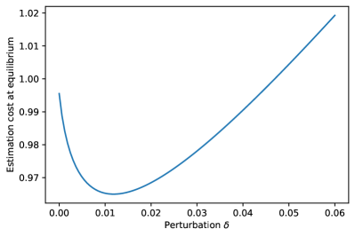
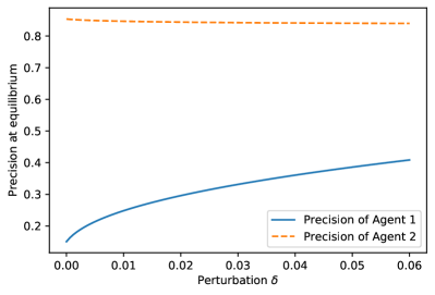
(a) Estimation cost	(b) Precision of agents

Figure 1: Counter-example 1: Estimation cost and precision of agents as a function of the perturbation $\delta$.

Example 2 (1-dimensional model with four agents).

We consider a $1$-dimensional game with four agents in which the public data of each agent equals $x_{i}=1$. Agents 1 and 2 have disclosure costs $c_{i}(\lambda)=\lambda^{1.01}$ while Agents 3 and 4 have disclosure costs $c_{i}(\lambda)=\lambda^{1.1}$. We consider a linear unbiased estimator that is equal to $\mathtt{GLS}$ plus a perturbation cost that only affects the first two agents: $D=[\sqrt{\delta},-\sqrt{\delta},0,0]$. Note that this perturbation is only applied to the most selfish agents as they are the ones we must incentivize to give more. We set the maximal precision to $1/\sigma^{2}=1$.

In Figure 2, we plot the estimation cost at equilibrium $f_{L(\delta)}(\boldsymbol{\lambda}^{*}_{L(\delta)})$ as a function of $\delta$. With $\mathtt{GLS}$ ($\delta=0$), we get an estimation cost of $0.9955$, which is larger than the value $0.9950$ that we obtain for $\delta=3.10^{-4}$. As for Example 1, when $\delta$ increases, the precisions used by the least generous agents (Agents 1 and 2) increase while the precisions of the most generous agents decrease.

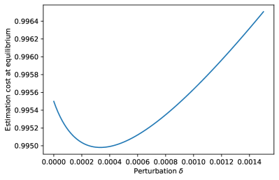
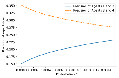
(a) Estimation cost	(b) Precision of agents

Figure 2: Counter-example 2: Estimation cost and precision of agents as a function of the perturbation $\delta$.

While the previous two counter-examples are in dimension 1 and with agents that all have $x_{i}=1$, the sub-optimality of $\mathtt{GLS}$ is not limited to that case. To illustrate that, we consider in the next counter-example models in dimension $d$ with $d\geq 2$. Note that, as we assume that matrix $X$ has rank $d$, we need at least $d$ players whose feature vectors $\boldsymbol{x}_{i}$’s span the $d$ dimensions. Note also that, with $d$ players in $d$ dimensions, $\mathtt{GLS}$ is the only linear unbiased estimator. Indeed, as matrix $X$ would then be invertible, the condition in (11) leads to $D^{T}=0$. In Example 3 below, we consider the simplest case of models with $d+1$ agents, though it is clear that one could construct similar counter examples with any number of agents larger than or equal to $d+1$.

Example 3 ($d$-dimensional models with $d+1$ agents).

We consider a $d$-dimensional game with $d+1$ agents. The public data of the first $d$ agents spans the $d$ dimensions: $\boldsymbol{x}_{i}$ is a vector where all components equal $0$ except the $i$th one that is equal to $1$. All components of the public data of Agent $d+1$ are equal to $1/d$: $\boldsymbol{x}_{d+1}=[1/d,\cdots,1/d]^{T}$. We assume that the disclosure costs of the first $d$ agents are $c_{i}(\lambda)=\lambda^{20}$ (for $i\in\{1,\cdots,d\}$), and the disclosure cost of the last agent is $c_{d+1}(\lambda)=\lambda^{1.5}$. We set the maximal precision to $1/\sigma^{2}=1$.

The perturbation matrix $D$ is a $(d+1)\times d$ matrix whose first column is $\sqrt{\delta}[1,\cdots,1,-d]$, all other entries being $0$. Hence, the public feature matrix $X$ and the perturbation matrix $D$ are the following $(d+1)\times d$ matrices:

$$X=\left[\begin{array}[]{cccc}1&&0\\ &\ddots&\\ 0&&1\\ 1/d&\dots&1/d\end{array}\right], D=\left[\begin{array}[]{cccc}\sqrt{\delta}&0&0&\dots\\ \vdots&0&0&\dots\\ \sqrt{\delta}&0&0&\dots\\ -d\sqrt{\delta}&0&0&\dots\end{array}\right].$$ (22)

It is easy to verify that $D^{T}X=0$, which implies $L(\delta)=\mathtt{GLS}+D^{T}$ is an unbiased estimator.

In Figure 3, we report the estimation cost at equilibrium $f_{L(\delta)}(\boldsymbol{\lambda}^{*}_{L(\delta)})$ as a function of $\delta$. We consider models of dimension $d\in\{2,5,10,15\}$. We observe that for all dimensions $d$, the behavior is similar to the one observed in Figure 1(a) and 2(a): when $\delta$ is small enough, using the estimator $L(\delta)$ provides a higher precision at equilibrium (i.e., a lower equilibrium estimation cost as seen on the graphs). This comes from the fact that when $\delta$ increases, the precision at equilibrium provided by Agent $d+1$ increases with $\delta$ whereas the precision provided by Agents $1$ to $d$ is almost independent of $\delta$. When $\delta$ increases too much, the estimation cost increases again because of the non-optimality of the estimator $L(\delta)$ (for given individual precisions). We also observe that the maximal gain that can be obtained by using an estimator other than $\mathtt{GLS}$ (and the perturbation $\delta$ for which it is achieved with our particular perturbation matrix $D$) seems to decrease when the dimension $d$ increases.

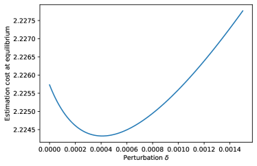
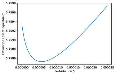
(a) $d=2$	(b) $d=5$
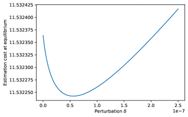
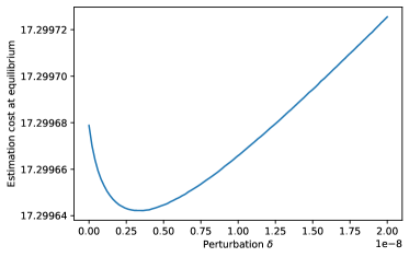
(c) $d=10$	(d) $d=15$

Figure 3: Counter-example 3: Estimation cost and precision of agents as a function of the perturbation $\delta$ for models in dimension $d\geq 2$.

Finally, although the public feature matrix $X$ in (22) has a particular form, many $d$-dimensional models with $d+1$ agents can be cast in this model via an appropriate change of basis. In fact, we conjecture that for any matrix of public features $X$ with at least $d+1$ agents, there exist disclosure costs such that $\mathtt{GLS}$ is not optimal.

7 Concluding Remarks

This paper studies linear regression in the presence of strategic data sources, modeling the precision choice as a non-cooperative game with a public good component. We establish existence of a unique non-trivial Nash equilibrium, and study its efficiency for a large class of disclosure and estimation cost functions. We also show an extension of the Aitken/Gauss-Markov theorem to this non-cooperative setup under certain conditions and examples in which the generalized least squares estimator is not optimal.

Our Aitken/Gauss-Markov-type theorem is weaker than these two classical results in three ways. First, we proved the generalized least squares estimator is only approximately optimal in the case of a homogeneous estimation cost and of near-homogeneous disclosure cost and is not always optimal. Second, the optimality of the generalized least squares estimator in the case of monomial disclosure cost functions of same degree is shown w.r.t. the homogeneous scalarization chosen, rather than the positive semidefinite order. Finally, Theorem 5 applies to linear estimators whose difference from $\mathtt{GLS}$ does not depend on the actions $\boldsymbol{\lambda}$. In the presence of arbitrary dependence on $\boldsymbol{\lambda}$, the non-trivial equilibrium need not be unique (or even exist). Understanding when this occurs, and proving optimality results in this context, also remains open.

Our model assumes that the precision chosen by each agent is known to the analyst. Amending this assumption brings issues of truthfulness into consideration: in particular, an important open question is whether there exists an estimator (viewed as a mechanism) that induces truthful precision reporting among agents, at least in equilibrium. An Aitken-type theorem seems instrumental in establishing such a result.

Our analysis of the Nash equilibrium assumes complete information, that is that agents know the costs and features of other agents. Extending it to a Bayesian setting is an interesting open direction. Still, even when the complete information assumption does not hold, our present results are indicative in at least two ways. First, as our game is a potential game, we know that many natural dynamic evolutions of the game will converge to the Nash equilibrium. Second, if the number of agents grows large, we expect that the Nash equilibrium and Bayesian Nash equilibrium would be close since the empirical distribution of costs/features would then be close to the true underlying distribution.

Appendix A Proof of Theorem 1

In this proof, we show that the potential function $\Phi$ is strictly convex on its effective domain which implies that the set of Nash equilibria that lie in its effective domain coincides with the set of local minima of $\Phi$. By strict convexity, $\Phi$ has at most one such local equilibrium. To conclude the proof, we then show that this minimum is attained.

The potential function $\Phi(\boldsymbol{\lambda})=f(\boldsymbol{\lambda})+\sum_{i}c_{i}(\lambda_{i})$ takes values in the extended positive real numbers line $\bar{\mathbb{R}}_{+}=\mathbb{R}_{+}\cup\{+\infty\}$. By Assumption 1, the disclosure costs $c_{i}(\cdot)$ are finite on $[0,1/\sigma^{2}]$ since they are continuous on a compact set. Therefore, $\Phi(\cdot)$ is finite if and only if $f(\cdot)$ is finite, i.e., $\operatorname{dom}\Phi\equiv\{\boldsymbol{\lambda}:\Phi(\boldsymbol{\lambda})<\infty\}=\operatorname{dom}f$, where $\operatorname{dom}$ is the effective domain. Recall that since $X$ has rank $d$, $(0,1/\sigma^{2}]^{n}\subseteq\operatorname{dom}\Phi$, and $\operatorname{dom}\Phi$ is non-empty.

Recall that $V(\boldsymbol{\lambda})=(X^{T}\Lambda X)^{-1}$. This implies that $V$ is strictly convex and goes to infinity when $A(\boldsymbol{\lambda})=X^{T}\Lambda X$ goes to a non-invertible matrix (i.e., the largest eigenvalue of $V$ goes to infinity for any sequence $\boldsymbol{\lambda}_{n}$ that converges to a $\boldsymbol{\lambda}$ such that $A(\boldsymbol{\lambda})$ is non-invertible). As $F$ is convex and increasing, this shows that $f(\boldsymbol{\lambda})=F(V(\boldsymbol{\lambda}))$ is strictly convex and goes to $+\infty$ when $A(\boldsymbol{\lambda})$ goes to a non-invertible matrix, which then implies that $f(\boldsymbol{\lambda}):[0,1/\sigma^{2}]^{n}\to\bar{R}_{+}$ is continuous. As the functions $c_{i}$ are convex, we conclude that the potential function $\Phi$ is strictly convex and continuous on $\bar{\mathbb{R}}_{+}$.

Let $B$ be the subset of $\boldsymbol{\lambda}$ such that $\Phi(\boldsymbol{\lambda})\leq\Phi(1/\sigma^{2}\dots 1/\sigma^{2})$. By continuity and convexity of $\Phi$, $B$ is a non-empty convex and compact subset of $[0,1/\sigma^{2}]^{n}$ on which $\Phi(\boldsymbol{\lambda})<\infty$. This implies that the unique minimum of $\Phi$ is attained in $B\subseteq\operatorname{dom}(\Phi)$. ∎

Appendix B Proof of Theorem 2

Under Assumptions 1 and 2, the unique non-trivial equilibrium $\boldsymbol{\lambda}^{*}$ minimizes the potential function $\Phi(\boldsymbol{\lambda})=\sum_{i\in N}c_{i}(\lambda_{i})+f(\boldsymbol{\lambda})$. Then, for $\boldsymbol{\lambda}^{\mathtt{opt}}$ a minimizer of the social cost:

$$\Phi(\boldsymbol{\lambda}^{*})\leq\Phi(\boldsymbol{\lambda}^{\mathtt{opt}})=\sum_{i\in N}c_{i}(\lambda_{i}^{\mathtt{opt}})+f(\boldsymbol{\lambda}^{\mathtt{opt}})\leq\sum_{i\in N}c_{i}(\lambda_{i}^{\mathtt{opt}})+nf(\boldsymbol{\lambda}^{\mathtt{opt}})=\mathtt{opt}$$

by the positivity of $f$. On the other hand, $C(\boldsymbol{\lambda}^{*})\leq n\Phi(\boldsymbol{\lambda}^{*})$, by the positivity of $c_{i}$, and the theorem follows. ∎

Appendix C Proof of Theorem 3

To simplify the notation, in this proof, we write $p$ instead of ${{p}_{\textrm{min}}}$; hence we show that $\mathtt{PoS}\leq n^{\frac{q}{p+q}}$.

Upper Bound. Recall that Assumption 3 implies that $\forall\lambda\in\mathbb{R}_{+},\forall a\geq 1,a^{p}c_{i}(\lambda)\leq c_{i}(a\lambda)$. This implies, by rewriting the assumption with $\lambda^{\prime}=a\lambda$, that $c_{i}(\frac{\lambda^{\prime}}{a})\leq a^{-p}c_{i}(\lambda^{\prime})$ for all $a\geq 1$ and for all $\lambda^{\prime}$.

Recall that we denote by $\boldsymbol{\lambda}^{*}$ the unique non-trivial Nash equilibrium. Suppose that $\mathtt{PoS}>n^{\frac{q}{p+q}}$, that is

$$\sum_{i\in N}c_{i}(\lambda^{*}_{i})+nf(\boldsymbol{\lambda}^{*}) >n^{\frac{q}{q+p}}(\sum_{i\in N}c_{i}(\lambda_{i}^{\mathtt{opt}})+nf(\boldsymbol{\lambda}^{\mathtt{opt}})).$$

We will show that this implies that $\boldsymbol{\lambda}^{*}$ is not an equilibrium, which is a contradiction.

By using that $c_{i}(\lambda^{*}_{i})\geq 0$ and dividing the above inequality by $n$, we obtain:

$$\sum_{i\in N}c_{i}(\lambda^{*}_{i})+f(\boldsymbol{\lambda}^{*}) \geq\frac{1}{n}\left(\sum_{i\in N}c_{i}(\lambda^{*}_{i})+nf(\boldsymbol{\lambda}^{*})\right)$$

$$>n^{-\frac{p}{q+p}}\sum_{i\in N}c_{i}(\lambda_{i}^{\mathtt{opt}})+n^{\frac{q}{p+q}}f(\boldsymbol{\lambda}^{\mathtt{opt}})$$

$$\geq\sum_{i\in N}c_{i}\left(\frac{\lambda_{i}^{\mathtt{opt}}}{n^{\frac{1}{p+q}}}\right)+f\left(\frac{\boldsymbol{\lambda}^{\mathtt{opt}}}{n^{\frac{1}{p+q}}}\right),$$

where for the last inequality, we used Assumption 3 and Assumption 4 with $a=n^{1/(p+q)}$.

To conclude the proof, we remark that $\frac{\boldsymbol{\lambda}^{\mathtt{opt}}}{n^{1/(p+q)}}\leq\boldsymbol{\lambda}^{\mathtt{opt}}$ which implies that $\frac{\boldsymbol{\lambda}^{\mathtt{opt}}}{n^{1/(p+q)}}$ is a valid strategy profile. This would imply that $\boldsymbol{\lambda}^{*}$ is not the minimum of the potential function which is a contradiction. Thus, we have $\mathtt{PoS}\leq n^{\frac{q}{p+q}}$.∎

Lower Bound. Fix $p\geq 1$ and $q\geq 1$. We consider a $1$-dimensional model ($d=1$) with $x_{1}=1$ and $\sigma^{2}=(q/p)^{1/(p+q)}$. Let $c_{i}(\lambda_{i})=\lambda_{i}^{p}$ for all $i$ and $F(V)=\operatorname{trace}(V)^{q}=V^{q}$ (the last equality holds because when $d=1$, the co-variance matrix is a scalar). Hence, the co-variance matrix is $V(\boldsymbol{\lambda})=(\sum_{i\in N}\lambda_{i})^{-1}$.

As all agents are identical, and by uniqueness of the Nash equilibrium, the Nash equilibrium is a symmetric Nash equilibrium where all agents will give the same value $\lambda^{*}$ where $\lambda^{*}$ is the unique minimizer of the potential function:

$$n\lambda^{p}+(n\lambda)^{-q}.$$

The minimum of this function is attained when its derivative is equal to $0$. This implies that $np\lambda^{p-1}=nq(n\lambda)^{-q-1}$ which implies that $\lambda^{p+q}=(q/p)n^{-1-q}$. This shows that $\lambda^{*}=((q/p)n^{-1-q})^{1/(p+q)}$.

Similarly, the socially optimal $\boldsymbol{\lambda}^{\mathtt{opt}}$ is also symmetric and is attained when all agents give $\lambda^{\mathtt{opt}}$ the unique minimizer of the social cost:

$$n\lambda^{p}+n(n\lambda)^{-q}.$$

This implies that

$$\lambda^{\mathtt{opt}}=(n(q/p)n^{-1-q})^{1/(p+q)}=n^{1/(p+q)}\lambda^{*}.$$ (23)

Hence, we get:

$$\mathtt{PoS} =\frac{C(\boldsymbol{\lambda}^{*})}{C(\boldsymbol{\lambda}^{\mathtt{opt}})}=\frac{n(\lambda^{*})^{p}+n(n\lambda^{*})^{-q}}{n(\lambda^{\mathtt{opt}})^{p}+n(n\lambda^{\mathtt{opt}})^{-q}}$$

$$=\frac{(\lambda^{*})^{p}+(n\lambda^{*})^{-q}}{(\lambda^{\mathtt{opt}})^{p}+(n\lambda^{\mathtt{opt}})^{-q}}$$

$$=\frac{(n\lambda^{*}){-q}}{(n\lambda^{\mathtt{opt}})^{-q}}\frac{(\lambda^{*})^{p+q}+1}{(\lambda^{\mathtt{opt}})^{p+q}+1}$$

$$=\left(\frac{\lambda^{\mathtt{opt}}}{\lambda^{*}}\right)^{q}\frac{1+(\lambda^{*})^{p+q}}{1+(\lambda^{\mathtt{opt}})^{p+q}}$$

$$=n^{q/(p+q)}\frac{1+(q/p)n^{-1-q}}{1+(q/p)n^{-q}},$$

where we use the expression in (23) for $\lambda^{*}$ and $\lambda^{\mathtt{opt}}$ in the last line. This shows that, for any $\epsilon$, for large enough $n$, the price of stability is at least $n^{q/(p+q)}(1-\varepsilon)$. ∎

Appendix D Proof of Theorem 5

D.1 Proof of (i)

We consider the same setting as Example 1, i.e., a $1$-dimensional model ($d=1$) with two agents in which the public data of each agent is $x_{i}=1$. For such a game, the $\mathtt{GLS}$ estimator is $(X^{T}\Lambda X)^{-1}X^{T}\Lambda\tilde{\boldsymbol{y}}=(\lambda_{1}+\lambda_{2})^{-1}\boldsymbol{\lambda}^{T}\tilde{\boldsymbol{y}}$ and its covariance is $1/(\lambda_{1}+\lambda_{2})$. We consider a linear estimator $\hat{\boldsymbol{\beta}}(\delta)$ with $\delta\geq 0$ of the form $\hat{\boldsymbol{\beta}}_{\mathtt{GLS}}+\boldsymbol{\delta}^{T}\tilde{\boldsymbol{y}}$ where $\boldsymbol{\delta}\in\mathbb{R}^{2}$ is a vector with coefficients $\delta_{1}=-\delta_{2}=\sqrt{\delta}$. Note that $\delta_{1}=-\delta_{2}$ guarantees that this linear estimator is unbiased. We assume that the disclosure cost of Agent 1 is $c_{1}(\lambda)=\lambda^{p_{1}}$ while the disclosure cost of Agent 2 is $c_{2}(\lambda)=\lambda^{p_{2}}$. For a given $\delta$, we denote the equilibrium of the game by $\boldsymbol{\lambda}^{*}(\delta)$.

Overall, this proof is decomposed in two steps:

Step 1: We compute the derivative of the estimation cost at $\delta=0$ to show that it is negative if and only if $\lambda^{*}_{1}(0)(2p_{1}-p_{2}-p_{1}p_{2})+\lambda^{*}_{2}(0)(2p_{2}-p_{1}-p_{1}p_{2})>0$.

Step 2: We show that there exists $x>0$ such that the above inequality is satisfied for $p_{1}=1/x$ and $p_{2}=1+x$.

We describe both steps in detail below.

Step 1.

According to (12), the covariance of the estimator is $1/(\lambda_{1}+\lambda_{2})+\delta/\lambda_{1}+\delta/\lambda_{2}$, where $\delta/\lambda_{1}+\delta/\lambda_{2}$ is the loss of precision due to using a linear estimator that is less precise than $\mathtt{GLS}$. We assume that the scalarization function is the identity, which means that the estimation cost is

$$f_{\delta}(\boldsymbol{\lambda})=\frac{1}{\lambda_{1}+\lambda_{2}}+\frac{\delta}{\lambda_{1}}+\frac{\delta}{\lambda_{2}}.$$ (24)

The equilibrium $\boldsymbol{\lambda}^{*}(\delta)$ is the minimum of the potential function $\Phi_{\delta}(\boldsymbol{\lambda})=f_{\delta}(\boldsymbol{\lambda})+\lambda_{1}^{p_{1}}+\lambda_{2}^{p_{2}}$. The estimation cost at equilibrium is $f_{\delta}(\boldsymbol{\lambda}^{*}(\delta))$. Our goal in this step is to compute the derivative of $f_{\delta}(\boldsymbol{\lambda}^{*}(\delta))$ with respect to $\delta$ and to obtain a condition that ensures that it is negative at $\delta=0$. Let use denote by $(\lambda^{*})^{\prime}_{i}(\delta)=d\lambda^{*}_{i}(\delta)/(d\delta)$ the derivative of $\lambda^{*}_{i}(\delta)$ with respect to $\delta$. To simplify notation, we will omit the dependence on $\delta$ and simply denote $\lambda^{*}_{i}=\lambda^{*}_{i}(0)$ and $\lambda_{i}^{\prime}=(\lambda^{*})^{\prime}_{i}(0)$ when it is not confusing. The derivative of the estimation cost evaluated at $\delta=0$ is equal to

$$\frac{d}{d\delta}(f_{\delta}(\boldsymbol{\lambda}^{*}(\delta)))\Big{|}_{\delta=0} =-\frac{\lambda^{\prime}_{1}+\lambda^{\prime}_{2}}{(\lambda^{*}_{1}+\lambda^{*}_{2})^{2}}+\frac{1}{\lambda^{*}_{1}}+\frac{1}{\lambda^{*}_{2}}=-\frac{\lambda^{\prime}_{1}+\lambda^{\prime}_{2}}{(\lambda^{*}_{1}+\lambda^{*}_{2})^{2}}+\frac{\lambda^{*}_{1}+\lambda^{*}_{2}}{\lambda^{*}_{1}\lambda^{*}_{2}}.$$ (25)

In particular, the above derivative is negative if an only if $\frac{\lambda^{\prime}_{1}+\lambda^{\prime}_{2}}{(\lambda^{*}_{1}+\lambda^{*}_{2})^{3}}\lambda^{*}_{1}\lambda^{*}_{2}>1$. In what follows, we compute the derivatives $\lambda_{i}^{\prime}$ as a function of the values of $\lambda^{*}_{i}$ and $p_{i}$.

The equilibrium $\boldsymbol{\lambda}^{*}(\delta)$ is the minimum of the potential function $\Phi_{\delta}(\boldsymbol{\lambda})=f_{\delta}(\boldsymbol{\lambda})+\lambda_{1}^{p_{1}}+\lambda_{2}^{p_{2}}$. By using the first order condition $\partial\Phi_{\delta}/\partial\lambda_{i}=0$, this implies that for all $\delta\geq 0$:

$$-\frac{1}{(\lambda^{*}_{1}(\delta)+\lambda^{*}_{2}(\delta))^{2}}-\frac{\delta}{(\lambda^{*}_{i}(\delta))^{2}}+p_{i}(\lambda^{*}_{i}(\delta))^{p_{i}-1}=0,\quad\text{for}~{}i\in\{1,2\}.$$ (26)

The derivative of $\lambda^{*}_{i}(\delta)$ with respect to $\delta$ exists thanks to the implicit function theorem. By differentiating (26) with respect to $\delta$, we obtain

$$0 =\frac{d}{d\delta}\left(-\frac{1}{(\lambda^{*}_{1}(\delta)+\lambda^{*}_{2}(\delta))^{2}}-\frac{\delta}{(\lambda^{*}_{i}(\delta))^{2}}+p_{i}(\lambda^{*}_{i}(\delta))^{p_{i}-1}\right)$$

$$=2\frac{(\lambda^{*})^{\prime}_{1}(\delta)+(\lambda^{*})^{\prime}_{2}(\delta)}{(\lambda^{*}_{1}(\delta)+\lambda^{*}_{2}(\delta))^{3}}-\frac{1}{(\lambda^{*}_{i}(\delta))^{2}}+2\delta\frac{(\lambda^{*})^{\prime}_{i}(\delta)}{(\lambda^{*}_{i}(\delta))^{3}}+p_{i}(p_{i}-1)(\lambda^{*}_{i}(\delta))^{p_{i}-2}(\lambda^{*})^{\prime}_{i}(\delta).$$ (27)

Equation (26), evaluated at $\delta=0$, shows that $p_{i}(\lambda^{*}_{i})^{p_{i}-1}=\frac{1}{(\lambda^{*}_{1}+\lambda^{*}_{2})^{2}}$. Evaluating Equation (27) at $\delta=0$ and plugging this equality gives

$$0 =2\frac{\lambda^{\prime}_{1}+\lambda^{\prime}_{2}}{(\lambda^{*}_{1}+\lambda^{*}_{2})^{3}}-\frac{1}{(\lambda^{*}_{i})^{2}}+p_{i}(p_{i}-1)(\lambda^{*}_{i})^{p_{i}-2}\lambda_{i}^{\prime}$$

$$=2\frac{\lambda^{\prime}_{1}+\lambda^{\prime}_{2}}{(\lambda^{*}_{1}+\lambda^{*}_{2})^{3}}-\frac{1}{(\lambda^{*}_{i})^{2}}+\frac{1}{(\lambda^{*}_{1}+\lambda^{*}_{2})^{2}}\frac{p_{i}-1}{\lambda^{*}_{i}}\lambda_{i}^{\prime}.$$ (28)

In order to isolate the term $\lambda_{1}^{\prime}+\lambda_{2}^{\prime}$, we multiply the above equation by $\lambda^{*}_{i}/(p_{i}-1)$ and we sum over $i\in\{1,2\}$. This gives:

$$0 =2\frac{\lambda_{1}^{\prime}+\lambda_{2}^{\prime}}{(\lambda^{*}_{1}+\lambda^{*}_{2})^{3}}\left(\frac{\lambda^{*}_{1}}{p_{1}-1}+\frac{\lambda^{*}_{2}}{p_{2}-1}\right)-\frac{1}{\lambda^{*}_{1}(p_{1}-1)}-\frac{1}{\lambda^{*}_{2}(p_{2}-1)}+\frac{\lambda^{\prime}_{1}+\lambda^{\prime}_{2}}{(\lambda^{*}_{1}+\lambda^{*}_{2})^{2}}$$

$$=\frac{\lambda_{1}^{\prime}+\lambda_{2}^{\prime}}{(\lambda^{*}_{1}+\lambda^{*}_{2})^{3}}\left(\frac{2\lambda^{*}_{1}}{p_{1}-1}+\frac{2\lambda^{*}_{2}}{p_{2}-1}+\lambda^{*}_{1}+\lambda^{*}_{2}\right)-\frac{1}{\lambda^{*}_{1}(p_{1}-1)}-\frac{1}{\lambda^{*}_{2}(p_{2}-1)}.$$

This shows that

$$\frac{\lambda_{1}^{\prime}+\lambda_{2}^{\prime}}{(\lambda^{*}_{1}+\lambda^{*}_{2})^{3}} =\frac{\frac{1}{\lambda^{*}_{1}(p_{1}-1)}+\frac{1}{\lambda^{*}_{2}(p_{2}-1)}}{\frac{2\lambda^{*}_{1}}{p_{1}-1}+\frac{2\lambda^{*}_{2}}{p_{2}-1}+\lambda^{*}_{1}+\lambda^{*}_{2}}$$

$$=\frac{1}{\lambda^{*}_{1}\lambda^{*}_{2}}\frac{\lambda^{*}_{2}(p_{2}-1)+\lambda^{*}_{1}(p_{1}-1)}{2\lambda^{*}_{1}(p_{1}-1)+2\lambda^{*}_{2}(p_{2}-1)+(\lambda^{*}_{1}+\lambda^{*}_{2})(p_{1}-1)(p_{2}-1)}.$$

In particular, this implies that the derivative (25) is negative if and only if

$$\frac{\lambda^{*}_{2}(p_{2}-1)+\lambda^{*}_{1}(p_{1}-1)}{2\lambda^{*}_{1}(p_{1}-1)+2\lambda^{*}_{2}(p_{2}-1)+(\lambda^{*}_{1}+\lambda^{*}_{2})(p_{1}-1)(p_{2}-1)}>1.$$

After some algebra, this gives

$$\lambda^{*}_{1}(2p_{1}-p_{2}-p_{1}p_{2})+\lambda^{*}_{2}(2p_{2}-p_{1}-p_{1}p_{2})>0,$$ (29)

where, again, by abuse of notation we denote $\lambda^{*}_{1}=\lambda^{*}_{1}(0)$ and $\lambda^{*}_{2}=\lambda^{*}_{2}(0)$.

Step 2.

We now consider $p_{1}=1+1/x$ and $p_{2}=1+x$ and $x\to\infty$. To emphasize the dependence in $x$, let us denote by $\boldsymbol{\lambda}^{*}(x)=(\lambda^{*}_{1}(x),\lambda^{*}_{2}(x))$ the value of the precision at equilibrium (for $\mathtt{GLS}$) and $\Phi_{x}(\cdot)$ the potential of the game. By definition, $\boldsymbol{\lambda}^{*}(x)$ minimizes $\Phi_{x}(\boldsymbol{\lambda})=1/(\lambda_{1}+\lambda_{2})+\lambda_{1}^{1+1/x}+\lambda_{2}^{1+x}$. This implies that for all $\epsilon>0$, $\Phi_{x}(\boldsymbol{\lambda}^{*}(x))\leq\Phi_{x}(0,1-\varepsilon)$. As $\lim_{x\to\infty}\Phi_{x}(0,1-\varepsilon)=1/(1-\varepsilon)$ and because this is true for all $\varepsilon$, this implies that

$$\lim_{x\to\infty}\Phi_{x}(\boldsymbol{\lambda}^{*}(x))=\lim_{x\to\infty}\left(\frac{1}{\lambda^{*}_{1}(x)+\lambda^{*}_{2}(x)}+(\lambda^{*}_{1}(x))^{1+1/x}+(\lambda^{*}_{2}(x))^{1+x}\right)\leq 1.$$

This implies that $\lim_{x\to\infty}\lambda^{*}_{1}(x)=0$ and $\lim_{x\to\infty}\lambda^{*}_{2}(x)=1$.

For our values of $p_{1}=1+1/x$ and $p_{2}=1+x$, the left-hand side of (29) equals $\lambda_{1}(x)(1/x-2x-1)+\lambda_{2}(x)(x-2/x-1)$. As $\lim_{x\to\infty}\lambda_{2}(x)=1$ and $\lim_{x\to\infty}\lambda_{1}(x)=0$, this term is asymptotically equivalent to $x$ and is therefore positive for $x$ large enough. This implies that there exists a value $x$ such that $d/(d\delta)f_{\delta}(\boldsymbol{\lambda}^{*}(\delta))<0$. Hence, for this $x$, there exists a perturbation value $\delta>0$ such that $\hat{\boldsymbol{\beta}}(\delta)$ is an estimator that is more efficient than $\mathtt{GLS}$. ∎

D.2 Proof of (ii)

We will start by proving Lemma 1. This lemma can easily be explained if we recall Assumption 3 and Assumption 4. Indeed, they dictate how the different components of the potential function behave when all agents multiply or divide the amount of information they give. If the sum of individual costs is too great compared to the common cost then dividing the amount that all agents give greatly reduces the individual costs while slightly augmenting the common cost, which is beneficial. The same goes the other way around where agents multiply the amount they give. This formalizes an intuition that one can have about this model: there is a balance between the individual costs paid to achieve the objective of reducing the common cost and the objective itself.

Lemma 1.

Under Assumptions 1, 2, 3 and 4, the ratio between the sum of individual costs and the common cost is bounded. Formally, the equilibrium $\boldsymbol{\lambda}^{*}$ satisfies:

$$\sum_{i\in N}c_{i}(\lambda^{*}_{i})\leq\frac{q}{{{p}_{\textrm{min}}}}f(\boldsymbol{\lambda}^{*})\text{\qquad and \qquad}f(\boldsymbol{\lambda}^{*})\leq\frac{{{p}_{\textrm{max}}}}{q}\sum_{i\in N}c_{i}(\lambda^{*}_{i}).$$

Proof.

This proof mainly relies on the fact that $\boldsymbol{\lambda}^{*}$ is the minimum of the potential function. Let $\boldsymbol{\lambda}^{*}$ be the unique non-trivial equilibrium. Let $\kappa\in(0,1)$ be a multiplicative factor applied to the equilibrium profile. As $\boldsymbol{\lambda}^{*}$ is the minimum of the potential function, we have $\Phi(\boldsymbol{\lambda}^{*})\leq\Phi(\kappa\boldsymbol{\lambda}^{*})$ and $\Phi(\boldsymbol{\lambda}^{*})\leq\Phi(\boldsymbol{\lambda}^{*}/\kappa)$. This implies that:

$$\sum_{i\in N}c_{i}(\lambda^{*}_{i})+f(\boldsymbol{\lambda}^{*}) \leq\sum_{i\in N}c_{i}(\kappa\lambda^{*}_{i})+f(\kappa\boldsymbol{\lambda}^{*})\leq\kappa^{{{p}_{\textrm{min}}}}\sum_{i\in N}c_{i}(\lambda^{*}_{i})+\kappa^{-q}f(\boldsymbol{\lambda}^{*}),\qquad\text{and}$$

$$\sum_{i\in N}c_{i}(\lambda^{*}_{i})+f(\boldsymbol{\lambda}^{*}) \leq\sum_{i\in N}c_{i}(\lambda^{*}_{i}/\kappa)+f(\boldsymbol{\lambda}^{*}/\kappa)\leq\kappa^{-{{p}_{\textrm{max}}}}\sum_{i\in N}c_{i}(\lambda^{*}_{i})+\kappa^{q}f(\boldsymbol{\lambda}^{*}).$$

The above equations imply that:

$$(1-\kappa^{{{p}_{\textrm{min}}}})\sum_{i\in N}c_{i}(\lambda^{*}_{i}) \leq(\kappa^{-q}-1)f(\boldsymbol{\lambda}^{*}),\qquad\text{and}$$

$$(1-\kappa^{q})f(\boldsymbol{\lambda}^{*}) \leq(\kappa^{-{{p}_{\textrm{max}}}}-1)\sum_{i\in N}c_{i}(\lambda^{*}_{i}).$$

As $\kappa\in(0,1)$, we have $1-\kappa^{{{p}_{\textrm{min}}}}>0$ and $\kappa^{-{{p}_{\textrm{max}}}}-1>0$. Hence, the above equations imply that

$$\frac{1-\kappa^{q}}{\kappa^{-{{p}_{\textrm{max}}}}-1}f(\boldsymbol{\lambda}^{*})\leq\sum_{i\in N}c_{i}(\lambda^{*}_{i}) \leq\frac{\kappa^{-q}-1}{1-\kappa^{{{p}_{\textrm{min}}}}}f(\boldsymbol{\lambda}^{*}).$$

This inequality is valid for every $\kappa\in(0,1)$. As $\lim_{\kappa\to 1}\frac{1-\kappa^{q}}{\kappa^{-{{p}_{\textrm{max}}}}-1}=q/{{p}_{\textrm{max}}}$ and $\lim_{\kappa\to 1}\frac{1-\kappa^{-q}}{1-\kappa^{-{{p}_{\textrm{min}}}}}=q/{{p}_{\textrm{min}}}$, this gives

$$\frac{q}{{{p}_{\textrm{max}}}}f(\boldsymbol{\lambda}^{*})\leq\sum_{i\in N}c_{i}(\lambda^{*}_{i})\leq\frac{q}{{{p}_{\textrm{min}}}}f(\boldsymbol{\lambda}^{*}).$$

∎

We are now ready to prove Theorem 5(ii). Let $\Phi_{L}(\boldsymbol{\lambda})=\sum_{i\in N}c_{i}(\lambda_{i})+f_{L}(\boldsymbol{\lambda})$ be the potential function for any linear unbiased estimator and $\Phi_{\mathtt{GLS}}(\boldsymbol{\lambda})=\sum_{i\in N}c_{i}(\lambda_{i})+f_{\mathtt{GLS}}(\boldsymbol{\lambda})$ be the potential function for $\mathtt{GLS}$. Recall that $\boldsymbol{\lambda}^{*}_{L}$ and $\boldsymbol{\lambda}^{*}_{\mathtt{GLS}}$ denote the non-trivial equilibria for the linear unbiased estimator and for $\mathtt{GLS}$ respectively. By optimality of $\mathtt{GLS}$, for all $\boldsymbol{\lambda}$ we have $f_{L}(\boldsymbol{\lambda})\geq f_{\mathtt{GLS}}(\boldsymbol{\lambda})$. This implies that for all $\boldsymbol{\lambda}$, we have $\Phi_{L}(\boldsymbol{\lambda})\geq\Phi_{\mathtt{GLS}}(\boldsymbol{\lambda})$. Therefore

$$\Phi_{L}(\boldsymbol{\lambda}^{*}_{L})=\min_{\boldsymbol{\lambda}}\Phi_{L}(\boldsymbol{\lambda})\geq\Phi_{\mathtt{GLS}}(\boldsymbol{\lambda}^{*}_{\mathtt{GLS}})=\min_{\boldsymbol{\lambda}}\Phi_{\mathtt{GLS}}(\boldsymbol{\lambda}).$$ (30)

By applying the inequalities of Lemma 1, we obtain:

$$\Phi_{\mathtt{GLS}}(\boldsymbol{\lambda}^{*}_{\mathtt{GLS}})=\sum_{i\in N}c_{i}((\boldsymbol{\lambda}^{*}_{\mathtt{GLS}})_{i})+f_{\mathtt{GLS}}(\boldsymbol{\lambda}^{*}_{\mathtt{GLS}})\geq\frac{q}{{{p}_{\textrm{max}}}}f_{\mathtt{GLS}}(\boldsymbol{\lambda}^{*}_{\mathtt{GLS}})+f_{\mathtt{GLS}}(\boldsymbol{\lambda}^{*}_{\mathtt{GLS}}),$$

and

$$\Phi_{L}(\boldsymbol{\lambda}^{*}_{L})=\sum_{i\in N}c_{i}((\boldsymbol{\lambda}^{*}_{L})_{i})+f_{L}(\boldsymbol{\lambda}^{*}_{L})\leq\frac{q}{{{p}_{\textrm{min}}}}f_{L}(\boldsymbol{\lambda}^{*}_{L})+f_{L}(\boldsymbol{\lambda}^{*}_{L}).$$

Combining the above two inequalities with (30), we conclude that

$$f_{\mathtt{GLS}}(\boldsymbol{\lambda}^{*}_{\mathtt{GLS}})\leq\frac{\frac{q}{{{p}_{\textrm{min}}}}+1}{\frac{q}{{{p}_{\textrm{max}}}}+1}f_{L}(\boldsymbol{\lambda}^{*}_{L})=\frac{{{p}_{\textrm{max}}}(q+{{p}_{\textrm{min}}})}{{{p}_{\textrm{min}}}(q+{{p}_{\textrm{max}}})}f_{L}(\boldsymbol{\lambda}^{*}_{L}).$$

References

- [1] Jacob Abernethy, Yiling Chen, Chien-Ju Ho, and Bo Waggoner. Low-cost learning via active data procurement. In Proceedings of the Sixteenth ACM Conference on Economics and Computation (EC ’15), pages 619–636, 2015.
- [2] Rakesh Agrawal and Ramakrishnan Srikant. Privacy-preserving data mining. In Proceedings of the 2000 ACM SIGMOD International Conference on Management of Data, pages 439–450, 2000.
- [3] A. C. Aitken. On least squares and linear combinations of observations. Proceedings of the Royal Society of Edinburgh, 55:42–48, 1935.
- [4] Mike Atallah, Elisa Bertino, Ahmed Elmagarmid, Mohamed Ibrahim, and Vassilios Verykios. Disclosure limitation of sensitive rules. In Workshop on Knowledge and Data Engineering Exchange (KDEX’99), pages 45–52, 1999.
- [5] A.C. Atkinson, A.N. Donev, and R.D. Tobias. Optimum experimental designs, with SAS. Oxford University Press New York, 2007.
- [6] Omer Ben-Porat and Moshe Tennenholtz. Regression equilibrium. In Proceedings of the 2019 ACM Conference on Economics and Computation (EC), pages 173–191, 2019.
- [7] S. Boyd and L. Vandenberghe. Convex Optimization. Cambridge University Press, 2004.
- [8] Y. Cai, C. Daskalakis, and C. H. Papadimitriou. Optimum statistical estimation with strategic data sources. In Proceedings of the 28th Annual Conference on Learning Theory (COLT 2015), pages 40.1–40.40, 2015.
- [9] Ioannis Caragiannis, Ariel D. Procaccia, and Nisarg Shah. Truthful univariate estimators. In Proceedings of the 33rd International Conference on Machine Learning (ICML ’16), 2016.
- [10] Yiling Chen, Nicole Immorlica, Brendan Lucier, Vasilis Syrgkanis, and Juba Ziani. Optimal data acquisition for statistical estimation. In Proceedings of the 2018 ACM Conference on Economics and Computation (EC), pages 27–44, 2018.
- [11] Yiling Chen, Chara Podimata, Ariel D. Procaccia, and Nisarg Shah. Strategyproof linear regression in high dimensions. In Proceedings of the 2018 ACM Conference on Economics and Computation (EC), pages 9–26, 2018.
- [12] Michela Chessa, Jens Grossklags, and Patrick Loiseau. A game-theoretic study on non-monetary incentives in data analytics projects with privacy implications. In Proceedings of the 28th IEEE Computer Security Foundations Symposium (CSF), 2015.
- [13] Michela Chessa and Patrick Loiseau. On non-monetary incentives for the provision of public goods, 2017. (Preprint. Available at https://ideas.repec.org/p/gre/wpaper/2017-24.html).
- [14] Anil Kumar Chorppath and Tansu Alpcan. Trading privacy with incentives in mobile commerce: A game theoretic approach. Pervasive and Mobile Computing, 9(4):598–612, 2013.
- [15] Rachel Cummings, Stratis Ioannidis, and Katrina Ligett. Truthful linear regression. In Proceedings of the 28th Annual Conference on Learning Theory (COLT 2015), volume 40, pages 1–36, 2015.
- [16] Pranav Dandekar, Nadia Fawaz, and Stratis Ioannidis. Privacy auctions for recommender systems. ACM Trans. Econ. Comput., 2(3):12:1–12:22, July 2014.
- [17] Anirban Dasgupta and Arpita Ghosh. Crowdsourced judgement elicitation with endogenous proficiency. In Proceedings of the 22nd International Conference on World Wide Web (WWW ’13), pages 319–330, 2013.
- [18] Ofer Dekel, Felix Fischer, and Ariel D. Procaccia. Incentive compatible regression learning. Journal of Computer and System Sciences, 76(8):759–777, 2010.
- [19] Josep Domingo-Ferrer. A survey of inference control methods for privacy-preserving data mining. In Privacy-preserving data mining, pages 53–80. Springer, 2008.
- [20] J.C. Duchi, M.I. Jordan, and M.J. Wainwright. Local privacy and statistical minimax rates. In Proceedings of the 54th IEEE Annual Symposium on Foundations of Computer Science (FOCS), pages 429–438, 2013.
- [21] George T Duncan and Sumitra Mukherjee. Optimal disclosure limitation strategy in statistical databases: Deterring tracker attacks through additive noise. Journal of the American Statistical Association, 95(451):720–729, 2000.
- [22] Cynthia Dwork. Differential privacy. In International Colloquium on Automata, Languages and Programming (ICALP), pages 1–12, 2006.
- [23] Rafael M. Frongillo, Yiling Chen, and Ian A. Kash. Elicitation for aggregation. In Proceedings of the 29th Conference on Artificial Intelligence (AAAI ’15), 2015.
- [24] Arpita Ghosh and Aaron Roth. Selling privacy at auction. In Proceedings of the 12th ACM Conference on Electronic Commerce (EC), pages 199–208, 2011.
- [25] Moritz Hardt, Nimrod Megiddo, Christos Papadimitriou, and Mary Wootters. Strategic classification. In Proceedings of the 2016 ACM Conference on Innovations in Theoretical Computer Science (ITCS ’16), pages 111–122, 2016.
- [26] Trevor Hastie, Robert Tibshirani, and Jerome Friedman. The Elements of Statistical Learning: Data Mining, Inference and Prediction. Springer, second edition, 2009.
- [27] Thibaut Horel, Stratis Ioannidis, and S Muthukrishnan. Budget feasible mechanisms for experimental design. In Proceedings of the 11th Latin American Theoretical INformatics Symposium (LATIN 2014), pages 719–730, 2014.
- [28] Safwan Hossain and Nisarg Shah. Pure nash equilibria in linear regression. Preprint, 2019.
- [29] Stratis Ioannidis and Patrick Loiseau. Linear regression as a non-cooperative game. In Proceedings of the 9th International Conference on Web and Internet Economics (WINE), pages 277–290, 2013.
- [30] Ramesh Johari and John N. Tsitsiklis. Efficiency loss in a network resource allocation game. Mathematics of Operations Research, 29(3):407–435, 2004.
- [31] Peter Kairouz, Sewoong Oh, and Pramod Viswanath. Extremal mechanisms for local differential privacy. Journal of Machine Learning Research, 17(17):1–51, 2016.
- [32] Daniel Kifer, Adam Smith, and Abhradeep Thakurta. Private convex empirical risk minimization and high-dimensional regression. In Proceedings of the 25th Annual Conference on Learning Theory (COLT 2012), pages 25.1–25.40, 2012.
- [33] Katrina Ligett and Aaron Roth. Take it or Leave it: Running a Survey when Privacy Comes at a Cost. In Proceedings of the 8th International Conference on Web and Internet Economics (WINE), pages 378–391, 2012.
- [34] Yang Liu and Yiling Chen. A bandit framework for strategic regression. In Advances in Neural Information Processing Systems 29 (NIPS), pages 1821–1829, 2016.
- [35] Yuan Luo, Nihar B. Shah, Jianwei Huang, and Jean Walrand. Parametric prediction from parametric agents. In Proceedings of the 10th Workshop on the Economics of Networks, Systems and Computation (NetEcon ’15), pages 57–57, 2015.
- [36] Reshef Meir, Ariel D. Procaccia, and Jeffrey S. Rosenschein. Algorithms for strategyproof classification. Artificial Intelligence, 186:123–156, 2012.
- [37] Dov Monderer and Lloyd S. Shapley. Potential games. Games and Economic Behavior, 14(1):124–143, 1996.
- [38] John Morgan. Financing public goods by means of lotteries. Review of Economic Studies, 67(4):761–84, October 2000.
- [39] Kobbi Nissim, Rann Smorodinsky, and Moshe Tennenholtz. Approximately optimal mechanism design via differential privacy. In Proceedings of the 3rd Innovations in Theoretical Computer Science Conference (ITCS), pages 203–213, 2012.
- [40] Stanley RM Oliveira and Osmar R Zaiane. Privacy preserving clustering by data transformation. In SBBD, pages 304–318, 2003.
- [41] Javier Perote and Juan Perote-Pena. Strategy-proof estimators for simple regression. Mathematical Social Sciences, 47(2):153–176, 2004.
- [42] F. Pukelsheim. Optimal design of experiments, volume 50. Society for Industrial Mathematics, 2006.
- [43] Tim Roughgarden and Éva Tardos. How bad is selfish routing? Journal of the ACM, 49(2):236–259, March 2002.
- [44] William H. Sandholm. Population Games and Evolutionary Dynamics. MIT Press, 2010.
- [45] Guido Schäfer. Online social networks and network economics. Lecture notes, Sapienza University of Rome, 2011.
- [46] Joseph F Traub, Yechiam Yemini, and H Woźniakowski. The statistical security of a statistical database. ACM Transactions on Database Systems (TODS), 9(4):672–679, 1984.
- [47] Jaideep Vaidya, Christopher W. Clifton, and Yu Michael Zhu. Privacy Preserving Data Mining. Springer, 2006.
- [48] Tyler Westenbroek, Roy Dong, Lillian J. Ratliff, and S. Shankar Sastry. Competitive statistical estimation with strategic data sources. IEEE Transactions on Automatic Control, 2019. To appear.