A Discontinuous Galerkin like Coarse Space correction for Domain Decomposition Methods with continuous local spaces: the DCS-DGLC Algorithm

Abstract

In this paper, we are interested in scalable Domain Decomposition Methods (DDM). To this end, we introduce and study a new Coarse Space Correction algorithm for Optimized Schwarz Methods(OSM): the DCS-DGLC algorithm. The main idea is to use a Discontinuous Galerkin like formulation to compute a discontinuous coarse space correction. While the local spaces remain continuous, the coarse space should be discontinuous to compensate the discontinuities introduced by the OSM at the interface between neighboring subdomains. The discontinuous coarse correction algorithm can not only be used with OSM but also be used with any one-level DDM that produce discontinuous iterates. While ideas from Discontinuous Galerkin(DG) are used in the computation of the coarse correction, the final aim of the DCS-DGLC algorithm is to compute in parallel the discrete solution to the classical non-DG finite element problem.

Résumé

Dans cet article, nous nous intéressons aux Méthods de Décomposition de Domaines (DDM) scalables. À cette fin, nous introduisons et étudions un nouvel algorithme, le DCS-DGLC, de correction grossière pour les méthodes de Schwarz optimisées. L’idée principale est d’utiliser une formulation apparentée aux méthodes de Galerkin discontinues pour calculer une correction grossière discontinue. Alors même que les espaces locaux restent continus, l’espace grossier est choisi discontinu afin de pouvoir compenser les discontinuités introduites par les OSM aux interfaces entre sous-domaines voisins. Cet algorithme de correction grossière discontinue peut être employé non seulement avec les OSM mais aussi avec toute DDM de un niveau qui produit des itérées discontinues. Bien que l’algorithme s’inspire des méthodes de Galerkin discontinues, le but final de l’agorithme est de calculer en parallèle la solution discrete à la formulation éléments finis classique, sans DG.

Introduction

During the second half of the $20$th century, the continuous increase in computing power was mainly due to increased sequential computing power. Parallel computers were very expensive and were rarely available to researchers. During the past decade, the situation changed as chip makers found it difficult to keep increasing the available sequential computing power. To keep offering continuously increasing computing power, they turned to parallelism by putting multiple cores in a single CPU. Nowadays, almost every computer that is sold contains a multicore CPU, even laptops, and is thus a parallel machine. It is therefore very important to design algorithms that can fully use this parallel computing power. At the same time, massively parallel computers also became increasingly affordable to the professional market. Instead of just a handful of nodes, massively parallel computers can consist of hundreds, thousands or tens of thousands of nodes. Parallel machines of up to ten thousands of nodes are now offered off the shelf and no longer need to be custom built. While these massively parallel computers remain, for the time being, still too expensive for the hobbyist, they can now be afforded by moderately rich research institutions. Because of the ever increasing availability of massively parallel computing power, it is no longer sufficient for algorithms to be parallel. To take advantage of the enormous parallel computing power of these machines, parallel algorithms must also be scalable. Scalability is the property for an algorithm to work well when more and more nodes are added. One usually distinguishes two kind of scalability:

Strong Scalability

The property for an algorithm to finish in half the time for a given problem size if the number of computation nodes is doubled.

Weak Scalability

The property for an algorithm to finish in the same amount of time if both the problem size and the number of computation nodes are doubled.

Strong Scalability is hard to achieve as when the number of nodes tends to infinity, the number of operation per processor would need to go to zero. In this paper, we are interested in the design of weakly scalable Domain Decomposition Methods.

Domain Decomposition Methods (DDM) are a family of algorithms designed to parallelize the computation of numerical solutions to Partial Differential Equations. These methods are designed with non shared memory architectures in mind. In Domain Decomposition Methods, the computation domain is subdivided in subdomains. In this paper, we only consider domain decompositions with no overlap between subdomains. In DDM, the interior equation is solved in parallel in each subdomain with artificial boundary conditions. Artificial boundary conditions are updated using information coming from the other subdomains. In one-level DDM, the update only uses information coming from the neighboring subdomains. One-level DDM can work fine when only a handful of subdomains are present. However, one-level DDM cannot be scalable. Since, the global solution often depends on what happens on the global domain, there can be no reasonable hope a one-level DDM will converge in less iterations than the diameter of the connectivity graph of the subdomain decomposition. This means that for $1D$ problems, or for $2D$ problems on a strip, we must iterate at least as many times as there are subdomains. Scalable Domain Decomposition Methods should have a convergence rate independent of the number of subdomains.

To get scalable Domain Decomposition Methods, some kind of global information transfer is needed. The standard way of making a DDM scalable is adding a coarse space to a pre-existing one-level DDM, thus making it a two-level DDM. The first use of coarse spaces in Domain Decomposition Methods can be traced back to [16]. Coarse spaces are used to send information globally: from any subdomain to all other subdomains. This global information transfer can be used to ensure scalability of the new DDM. Among well known DDM with coarse spaces are the two-level Additive Schwarz method [2], the FETI method [13], and the balancing Neumann-Neumann methods [12, 3, 14]. See [18, 17] for complete analyses of such methods. Coarse spaces are currently an active area of research, for example for high contrast problems [1, 15]. Adding an effective coarse space to Optimized Schwarz Methods (OSM), or to any one-level DDM that produce discontinuous iterates, is also highly non trivial: see [5], [4, chap.5] for numerous numerical tests, and [6] for a rigorous analysis of a special case.

For domain decomposition methods that produce discontinuous iterates at the interface between subdomains, it is advantageous that the coarse space be discontinuous at the interfaces between subdomains. In [10], Discontinuous Coarse Spaces (DCS) were advocated. In the same paper, was also introduced the DCS-DMNV (DCS-Dirichlet Minimizer Neumann Variational) algorithm that computed a discontinuous coarse correction for the Optimized Schwarz Method (OSM) in FEM-based discretizations. See [8] for a description and analysis of OSM. For a similar approach to adding an efficient coarse space to the Restricted Additive Schwarz (RAS) algorithm, see also [9]. See [7] for an analysis of the one-level RAS algorithm.

In this paper, we introduce and analyze another two-level Domain Decomposition Method: the DCS-DGLC (DCS-Discontinuous Galerkin Like Correction) algorithm. Like the DCS-DMNV algorithm introduced in [10], the DCS-DGLC algorithm makes use of Discontinuous Coarse Spaces, is suitable to Finite Element discretizations, and designed to not need Krylov acceleration to converge. The coarse correction step iself is different. In particular, in the DCS-DGLC, the computation of the coarse correction is inspired by the ideas present in Discontinuous Galerkin and uses a penalization function in the variational formulation at the coarse level. Even though ideas from Discontinuous Galerkin are used, the goal of the DCS-DGLC algorithm is to converge to the discrete solution of the non discontinuous Galerkin finite elements formulation. It is probable the coarse space algorithm could be adapted to a true DG formulation but this goes far beyond the scope of this paper. In this paper, we only consider the $(\eta-\operatorname{\triangle})u=0$ equation, both OSM and the DCS-DGLC algorithm can be adapted to more general elliptic operators.

In §1, we remind the readers about some previously known ideas, results or algorithms concerning Domain Decomposition Methods and coarse spaces that are useful to understand the DCS-DGLC algorithm. Then, in §2, we state the DCS-DGLC algorithm and explain the motivations and the ideas behind this algorithm. Then, in §3, we present some numerical results for both the iterative version in §3.1 and the Krylov accelerated version in §3.2.

1 Optimized Schwarz Methods and Discontinuous Coarse spaces

In this section, we recall the formulation of Optimized Schwarz Methods, the ideas behind the use of Discontinuous Coarse Spaces (DCS), and the DCS-DMNV [10] algorithm.

Let $\Omega$ be a bounded domain of $\mathbb{R}^{d}$. Let $(\Omega_{i})_{1\leq i\leq N}$ be a non overlapping domain decomposition of $\Omega$. The one-level Optimized Schwarz Methods are defined by

Algorithm 1.1 (One-level Optimized Schwarz).

1. Set an initial $u_{i}^{0}$. Until convergence

   1. Set $u_{i}^{n+1}$ as the unique solution to

      $$(\eta-\operatorname{\triangle})u_{i}^{n+1} =f\quad\text{in $\Omega_{i}$}$$

      $$\mathcal{B}_{ij}u_{i}^{n+1} =\mathcal{B}_{ij}u_{j}^{n}\quad\text{on $\partial\Omega_{i}\cap\partial\Omega_{j}$}$$

      $$u_{i}^{n+1} =0\quad\text{on $\partial\Omega_{i}\cap\partial\Omega$}$$

As explained in the introduction, one-level Optimized Schwarz Methods cannot be scalable. To make them two-level and scalable, we need a coarse space. Such a coarse space should contain discontinuous functions. The motivations behind the use of discontinuous coarse spaces can be found in details in [10]. The basic idea is that since many DDM, and in particular Opimized Schwarz Methods (OSM), introduce discontinuities at the interfaces between subdomains, we need coarse functions with discontinuities also located at the interface between subdomains to compensate those discontinuities. To understand why, consider a generic iterative Coarse Space Correction algorithm:

Algorithm 1.2 (Generic Coarse Space Correction Algorithm).

1. Choose a coarse space $X$.

2. Initialize $u_{i}^{0}$, either by zero or using the coarse solution.

3. For $n\geq 0$ and until convergence

   1. In each subdomain $\Omega_{i}$, compute the local iterates $u_{i}^{n+1/2}$ in parallel using the optimized Schwarz algorithm.

   2. Compute a coarse correction $U^{n+1}$ belonging to a coarse space $X$.

   3. Set the global iterates to $u_{i}^{n+1}:=u_{i}^{n+1/2}+U^{n+1}$.

4. Set either $u_{i}:=u_{i}^{n-1/2}$ or $u_{i}:=u_{i}^{n}$ where $n$ is the exit index of the above loop.

In the above algorithm, we haven’t specified yet how to compute $U^{n+1}$. More important than the algorithm used to compute $U^{n+1}$ is the choice of the coarse space $X$ itself. A function $u$ in $\otimes_{i=1}^{N}H^{1}(\Omega_{i})$ is a weak solution to the linear elliptic equation $\eta-\operatorname{\triangle}u=f$ on $\Omega$ if and only if

1. for all subdomains $\Omega_{i}$, $u_{|\Omega_{i}}$ is a weak solution to the interior equation $(\eta-\operatorname{\triangle})u=f$ inside subdomain $\Omega_{i}$.

2. there is no Dirichlet jumps, i.e., $u_{i}=u_{j}$ on $\partial\Omega_{i}\cap\partial\Omega_{j}$.

3. there is no Neuman jumps, i.e., $\frac{\partial u_{i}}{\partial\bm{n}_{i}}+\frac{\partial u_{i}}{\partial\bm{n}_{i}}=0$ on $\partial\Omega_{i}\cap\partial\Omega_{j}$.

The coarse step in the algorithm should give global iterates $u_{i}^{n+1}$ that are closer to satisfying these three conditions that the local iterates $u_{i}^{n+1/2}$. Since the interior equation is already satisfied inside each subdomain by the local iterates, no improvement is possible there. The best that can be achieved is for the global iterates to also satisfy the interior equation inside each subdomains. Therefore, the coarse space elements should satisfy the homogenous interior equation inside each subdomains. If the coarse space $X$ was a subset of $H^{1}(\Omega)$, then the Dirichlet jumps of the global iterates across subdomains would be equal to the Dirichlet jumps of the local iterates and there could be no improvement. If the global iterates are to have lower Dirichlet jumps across subdomains than the local iterates, then the coarse space $X$ must contain discontinuous functions. This is why, the coarse space $X$ should always be a subset of

$$\mathcal{A}=\{u\in H^{1,disc}_{0}(\Omega),\ \forall i,\ (\eta-\triangle)u_{|\Omega_{i}}=0\}.$$

The space $\mathcal{A}$ is small for one-dimensional problems but very big for two or higher dimensional problems. hence, using the full optimal theoretical coarse space $\mathcal{A}$ is unpractical in to or higher dimensions. Using of a suspace $X$ of small dimension as the coarse space is necessary.

To our knowledge, the first discontinuous coarse space correction algorithm that didn’t need Krylov acceleration to converge for Optimized Schwarz Methods is the DCS-DMNV (DCS- Dirichlet Minimizer Neumann Variational) algorithm. See [10] for a description and analysis. We reproduce the DCS-DMNV algorithm here:

Algorithm 1.3 (DCS-DMNV).

1. Choose a coarse space $X_{d}$. Set $X_{c}=X_{d}\cap H^{1}(\Omega)$.

2. Initialize $u_{i}^{0}$ by either zero or $u^{0}_{|\Omega_{i}}$ where $u^{0}$ is the coarse solution.

3. Until convergence

   1. Compute in parallel the local iterates $u_{i}^{n+1/2}\in H^{1}(\Omega_{i})$ from the global iterates $u_{i}^{n}$ using Optimized Schwarz.

   2. Define a global $u^{n+1/2}\in H^{1,disc}_{0}(\Omega)$ as $u_{i}^{n+1/2}$ in $\Omega_{i}$. Set $U^{n+1}$ as the unique function in $X_{d}$ such that

      $$q(u^{n+1/2}+U^{n+1})=\min_{v\in X_{d}}q(u^{n+1/2}+v),$$ (1a)

      with $$q(u)=\sum_{ij}\int_{\partial\Omega_{i}\cap\partial\Omega_{j}}\lvert u_{i}-u_{j}\rvert^{2}\mathrm{d}\sigma(\bm{x})$$, and satisfying

      $$\eta\int_{\Omega}U^{n+1}(x)v(x)\mathrm{d}x+\int_{\Omega}\nabla U^{n+1}(x)\nabla v(x)\mathrm{d}x-\sum_{i,j}\int_{\partial\Omega_{i}\cap\partial\Omega_{j}}\left(\frac{\partial u_{i}^{n+1/2}}{\partial n_{i}}+\frac{\partial u_{j}^{n+1/2}}{\partial n_{j}}\right)v\mathrm{d}\sigma,$$

      for all test functions $$v X_{c}$$ in .

   3. Set $u_{i}^{n+1}:=u_{i}^{n+1/2}+U^{n+1}$.

4. Set $u:=u_{i}^{n-1/2}$ on $\Omega_{i}$ for each $i$ in $\{1,\ldots,N\}$.

In the DCS-DMNV algorithm the discontinuous coarse correction was computed by choosing the unique coarse corrector that minimized the $L^{2}$ norm of the Dirichlet jump and satisfied the weak formulation for coarse test functions. Test functions needs to be $H^{1}$ in the variational formulation. Besides, for symmetric problems, it was advantageous to choose the intersection between the coarse space and $H^{1}$ as the set of test functions. This added the requirement that the coarse space contained a sufficiently large “continuous” subset. In the next section, we introduce a new algorithm, the DCS-DGLC algorithm, in which the coarse correction problem no longer requires test functions that belongs to $H^{1}(\Omega)$.

2 The DCS-DGLC algorithm

Our goal is to design another discontinuous coarse space correction algorithm for OSM that can use discontinuous test functions. Inspired by Discontinuous Galerkin formulations, we remove the Dirichlet jump minimization. As in Discontinuous Galerkin methods, a penalization parameter $q>0$ is introduced in front of a boundary term that penalizes jumps across the interfaces between neighboring subdomains. All functions in the coarse space can now be used as test functions for the coarse problems instead of just those that happen to also be $H^{1}$.

Algorithm 2.1 (DCS-DGLC).

1. Choose a coarse space $X$.

2. Initialize $u_{i}^{0}$ by either zero or $u^{0}_{|\Omega_{i}}$ where $u^{0}$ is the coarse solution.

3. Until convergence

   1. Compute in parallel the local iterates $u_{i}^{n+1/2}\in H^{1}(\Omega_{i})$ from the global iterates $u_{i}^{n}$ using Optimized Schwarz.

   2. Define a global $u^{n+1/2}\in H^{1,disc}_{0}(\Omega)$ as $u_{i}^{n+1/2}$ in $\Omega_{i}$.

   3. Set $U^{n+1}$ as the unique function in $X$ such that

      $$\begin{split}&\phantom{=}\sum_{i=1}^{N}\eta\int_{\Omega}U^{n+1}(x)V(x)\mathrm{d}x+\sum_{i=1}^{N}\int_{\Omega}\nabla U^{n+1}(x)\nabla V(x)\mathrm{d}x\\ \\ &\phantom{=}+q\sum_{ij}\int_{\Gamma_{ij}}(u_{i}^{n+1/2}+U_{i}^{n+1}-u_{j}^{n+1/2}-U_{j}^{n+1})\cdot(V_{i}-V_{j})\mathrm{d}\sigma(\hat{\bm{x}})\\ &=-\sum_{ij}\int_{\partial\Omega_{i}\cap\Omega_{j}}\theta\left(\frac{\partial u_{i}^{n+1/2}}{\partial n_{i}}+\frac{\partial u_{j}^{n+1/2}}{\partial n_{j}}\right)(V_{i}+V_{j})\mathrm{d}\sigma(\hat{\bm{x}}),\end{split}$$ (2)

      for all test functions $V$ in $X$.

   4. Set $u_{i}^{n+1}:=u_{i}^{n+1/2}+U^{n+1}$.

4. Set $u:=u_{i}^{n-1/2}$ on $\Omega_{i}$ for each $i$ in $\{1,\ldots,N\}$.

As the DCS-DMNV algorithm, the DCS-DGLC is suitable for Finite Element based discretizations. However, contrary to the DCS-DMNV algorithm, test functions need not be $H^{1}(\Omega)$. This is advantageous for symmetric problems as it lifts the requirement that the continuous subset of the discontinuous coarse space has to be big enough.

To choose the value of $\theta$, one could get inspiration from the Neumann-Neumann methods that also involve jumps of the Neumann boundary conditions, we could choose to set $\theta=1/4$ on non crosspoints and $\theta=1/K^{2}$ at crosspoints where $K$ equals the number of subdomains that meats at that particular crosspoints, see [18, ch. 6]. For ease of implementation, we chose $\theta=1/\max(K)^{2}$ where $\max(K)$ is the maximum over all crosspoints of the number of subdomains that meet at that given crosspoint.

3 Numerical Results

In this section, we show convergence curves for the DCS-DGLC algorithm when solving $-\operatorname{\triangle}u=f$ with homogenous Dirichlet conditions in $[0,4]^{2}$. We consider $Q_{1}$ finite elements on a cartesian mesh. We have $5\times 5$ subdomains and $50\times 50$ cells per subdomains. We iterate on the errors: we start with $f=0$ but also with random Robin boundary conditions on each subdomain. This has the advantage, for the iterative DCS-DGLC, of having the machine precision plateau given not by the machine epsilon but by its underflow level. This is not the case for the GMRES accelerated version. The error curves always show the $\log_{10}$ of the $L^{\infty}$ norm of the error.

Unfortunately, for “historical reasons”, our implementation can only use one particular piecewise harmonic discontinuous coarse space. This space is constructed by taking linear Dirichlet boundary conditions on each edge of a subdomain, then solving the homogenous equation. In that particular run of tests, we chose $\eta=0$, so this gives a discontinuous $Q_{1}$ coarse space. This coarse space happens to have a large $H^{1}$ subset. Future implementations won’t have this limitation.

When using Optimized Schwarz on finite elements, it is important that the Robin boundary conditions be lumped, see [11]. Without lumping the Robin boundary part of the rigidity matrix, we would observe slow modes.

3.1 Iterative DCS-DGLC algorithm

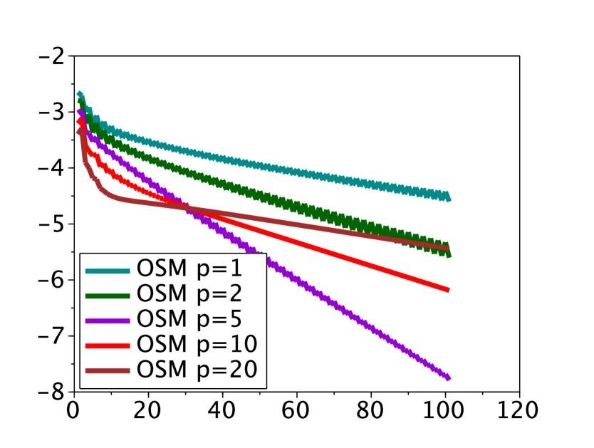
(a) One-level

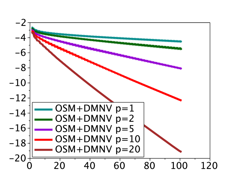
(b) DCS-DMNV

Figure 1: Convergence rates for the one-level OSM and DCS-DMNV

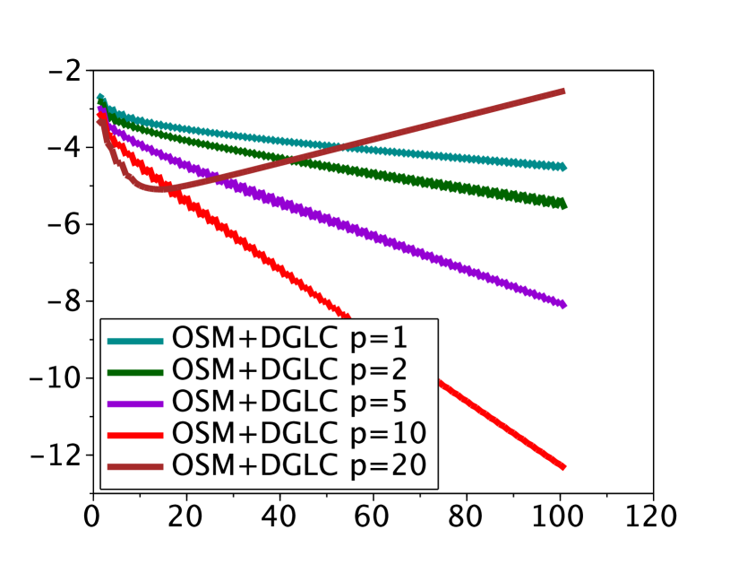
(a) $q=1$

(b) $q=100$

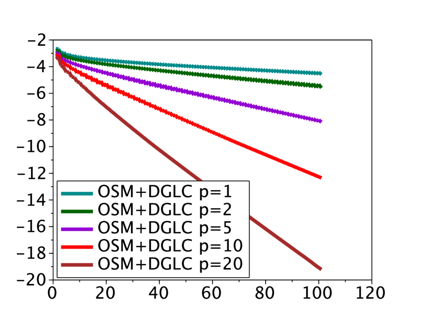
(c) $q=10000$

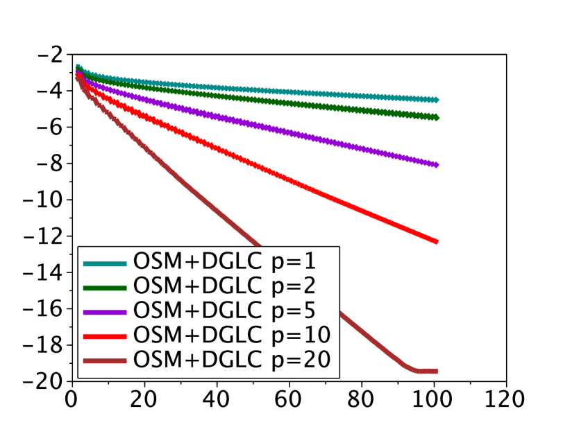
(d) $q=10$

(e) $q=1000$

(f) $q=100000$

Figure 2: Convergence rates for the DCS-DGLC Algorithm

In this section, we show error curves for the iterative DCS-DGLC algorithm with six different values for the penalization parameter $q$, see Figure 2. To give reference points for the performance of the algorithm, we also show convergence curves for the one-level OSM and the DCS-DMNV, see Figure 1. First we observe that convergence is much slower for the one-level OSM, see Figure 1, which was to be expected. We also observe that for $q=1$ and of $p=20$, the iterative DCS-DGLC algorithm diverges, see Figure 2. For all the other values of $p$ and $q$, we observe convergence. The performance of the DCS-DGLC is very close to the performance of the DCS-DMNV algorithm, see Figure 1. In all cases both two-level algorithm converge much faster than the one-level algorithm. For $p=20$, they reach an error of $10^{-20}$ in $100$ iterations. We also observe that the behavior of the DCS-DGLC algorithm seems to depend very little on $q$ once $q\geq 10$.

3.2 Krylov acceleration

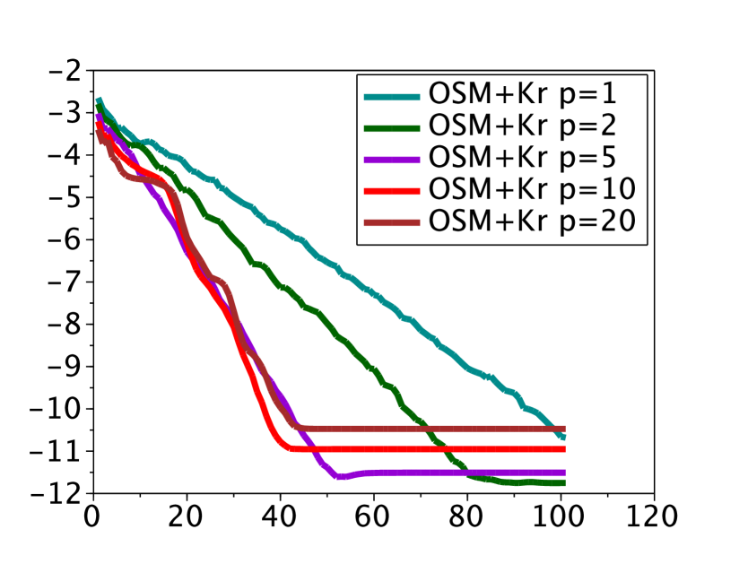
(a) One-level

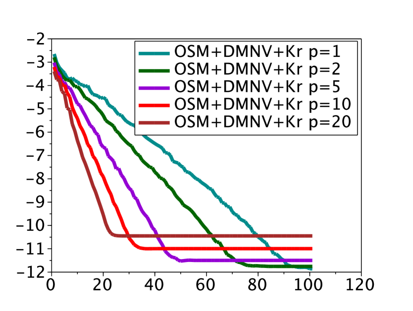
(b) DCS-DMNV

Figure 3: Convergence rates for the one-level OSM and DCS-DMNV with GMRES acceleration

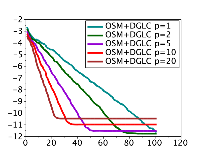
(a) $q=1$

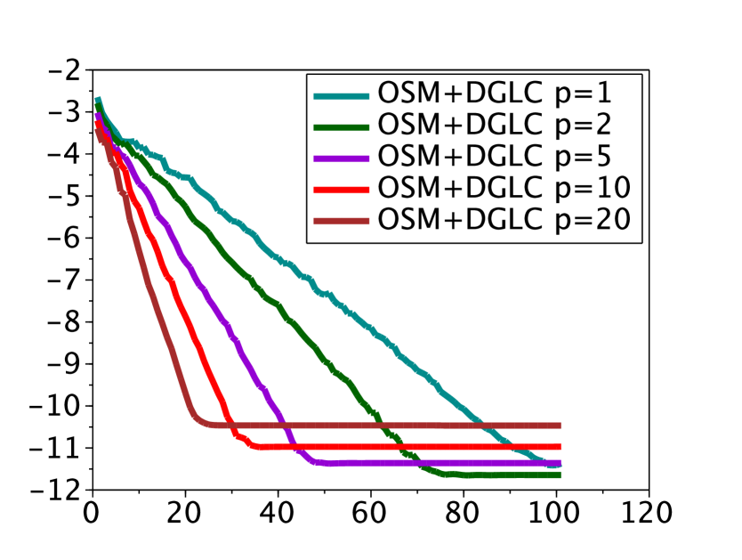
(b) $q=100$

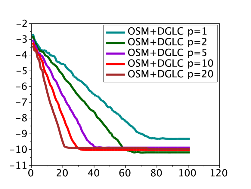
(c) $q=10000$

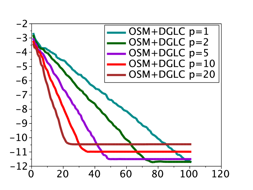
(d) $q=10$

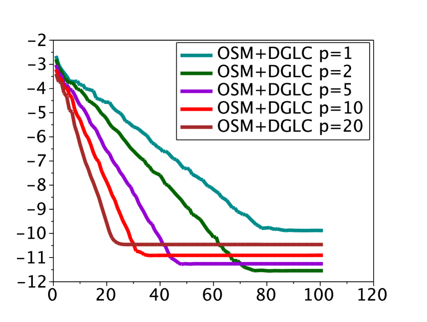
(e) $q=1000$

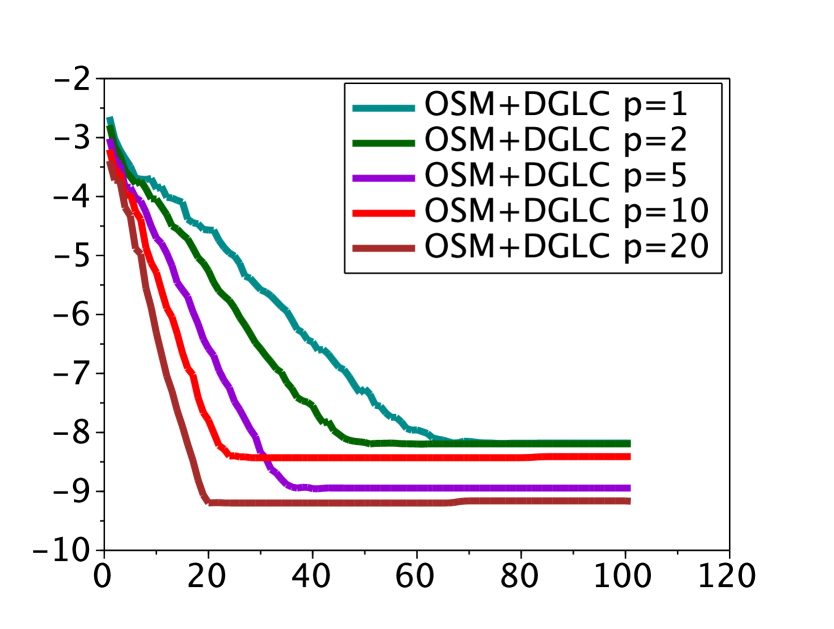
(f) $q=100000$

Figure 4: Convergence rates for the DCS-DGLC Algorithm with GMRES acceleration

It is well known that Domain Decomposition Methods can also be accelerated using Krylov methods. The classical idea that applies to any iterative method is to see the iteration $u^{n+1}=Bu^{n}+b$ as a Richardson method to solve $(I-B)u=b$ and to apply a Krylov method on $I-B$. While such acceleration gives faster methods, it is not sufficient to achieve scalable DDM. In practice, one should always apply Krylov acceleration. However, for the purpose of analysing an algorithm, it can be best to study the numerical behavior of the iterative DDM itself. Krylov acceleration is so efficient it often hides away small design errors in a DDM algorithm. On the contrary, the slightest design error often causes most iterative algorithms to fail. This makes it easier to detect a DDM is non optimal and should be improved. Nevertheless, we feel we wouldn’t provide a complete picture without providing results of numerical simulations in a Krylov setting. It is important to note that Krylov acceleration cannot by itself make a one-level DDM scalable.

In this section, we show error curves for the GMRES accelerated DCS-DGLC algorithm with six different values for the penalization parameter $q$, see Figure 4. To give reference points for the performance of the algorithm, we also show convergence curves for the GMRES accelerated one-level OSM and the GMRES accelerated DCS-DMNV, see Figure 3. Because of how GMRES works, we reach a plateau that depends on the machine epsilon even though we are iterating on the errors. The GMRES accelerated versions converge much faster than their iterative counterparts. As expected, the one-level method is the slowest. One advantage of the GMRES accelerated DCS-DGLC is that it converges well even when $q=1$ and $p=20$. The performance of the accelerated DCS-DGLC algorithm seems to depend very little on $q$, however, the numerical plateau due to rounding errors is higher for high values of $q$.

Conclusion

We have introduced a new discontinuous coarse space algorithm, the DCS-DGLC, that can be used with any one-level Domain Decomposition Methods that produce discontinuous iterates. We implemented that algorithm when used in conjunction with Optimized Schwarz Methods, a subfamily of Domain Decomposition Methods. Like its predecessor, the DCS-DMNV, which was the subject of a previous paper, the DCS-DGLC is designed to work well with Finite Element Discretizations. One potential advantage of the DCS-DGLC over the DCS-DMNV is that it does not in theory needs that the coarse space contain a significant “continuous” subset. One advantage of lifting the “sizable continuous subset” requirement is that it allows non Dirichlet boundary conditions to be used to construct discontinuous coarse space elements that also satisfy the interior equation inside each subdomain. Unfortunately, due to the limitations of our implementation, we weren’t able to study the numerical behavior of the DCS-DGLC algorithm when the coarse space has a trivial “continuous” subspace. We plan to do so in the future.

References

- [1] Victoria Dolean, Frédéric Nataf, Robert Scheichl, and Nicole Spillane. Analysis of a two-level schwarz method with coarse spaces based on local dirichlet to neumann maps. Computational Methods in Applied Mathematics, 12(4):391–414, 2012.
- [2] Maksymilian Dryja and Olof B. Widlund. An additive variant of the Schwarz alternating method for the case of many subregions. Technical Report 339, also Ultracomputer Note 131, Department of Computer Science, Courant Institute, 1987.
- [3] Maksymilian Dryja and Olof B. Widlund. Schwarz methods of Neumann-Neumann type for three-dimensional elliptic finite element problems. Comm. Pure Appl. Math., 48(2):121–155, February 1995.
- [4] Olivier Dubois. Optimized Schwarz Methods for the Advection-Diffusion Equation and for Problems with Discontinuous Coefficients. PhD thesis, McGill University, 2007.
- [5] Olivier Dubois and Martin J. Gander. Convergence behavior of a two-level optimized Schwarz preconditioner. In Domain Decomposition Methods in Science and Engineering XXI. Springer LNCSE, 2009.
- [6] Olivier Dubois, Martin J. Gander, Sebastien Loisel, Amik St-Cyr, and Daniel Szyld. The optimized Schwarz method with a coarse grid correction. SIAM J. on Sci. Comp., 34(1):A421–A458, 2012.
- [7] Evridiki Efstathiou and Martin J. Gander. Why Restricted Additive Schwarz converges faster than Additive Schwarz. BIT Numerical Mathematics, 43(5):945–959, 2003.
- [8] Martin J. Gander. Optimized Schwarz methods. SIAM J. Numer. Anal., 44(2):699–731, 2006.
- [9] Martin J. Gander, Laurence Halpern, and Kévin Santugini. A new coarse grid correction for RAS. In Domain Decomposition Methods in Science and Engineering XXI. Springer LNCSE, 2013.
- [10] Martin J. Gander, Laurence Halpern, and Kévin Santugini-Repiquet. Discontinuous coarse spaces for dd-methods with discontinuous iterates. In Domain Decomposition Methods in Science and Engineering XXI. Springer LNCSE, 2013.
- [11] Martin J. Gander, Florence Hubert, and Stella Krell. Optimized Schwarz algorithm in the framework of DDFV schemes. In Domain Decomposition Methods in Science and Engineering XXI. Springer LNCSE, 2013. submitted.
- [12] Jan Mandel. Balancing domain decomposition. Communications in Numerical Methods in Engineering, 9(3):233–241, mar 1993.
- [13] Jan Mandel and Marian Brezina. Balancing domain decomposition for problems with large jumps in coefficients. Math. Comp., 65:1387–1401, 1996.
- [14] Jan Mandel and Radek Tezaur. Convergence of a Substructuring Method with Lagrange Multipliers. Numer. Math., 73:473–487, 1996.
- [15] Frédéric Nataf, Hua Xiang, Victorita Dolean, and Nicole Spillane. A coarse sparse construction based on local Dirichlet-to-Neumann maps. SIAM J. Sci. Comput., 33(4):1623–1642, 2011.
- [16] Roy A. Nicolaides. Deflation conjugate gradients with application to boundary value problems. SIAM J. Num. An,, 24(2):355–365, 1987.
- [17] Barry F. Smith, Petter E. Bjørstad, and William Gropp. Domain Decomposition: Parallel Multilevel Methods for Elliptic Partial Differential Equations. Cambridge University Press, 1996.
- [18] Andrea Toselli and Olof Widlund. Domain Decomposition Methods - Algorithms and Theory, volume 34 of Springer Series in Computational Mathematics. Springer, 2004.