Geometric phase of neutrino propagating through dissipative matter

Abstract

We study the geometric phase (GP) in neutrino oscillation for both Dirac and Majorana neutrinos. We apply the kinematic generalization of the GP to quantum open systems that take into account the coupling to a dissipative environment. In the dissipationless case, the GP does not depend on the Majorana angle. It is not the case in the presence of dissipation and hence the GP can serve as a tool determining the type of the Dirac vs the Majorana neutrino.

The physics of neutrino has inspired the long-standing debate, at least in two clearly recognizable issues. The first is related to the existence of the neutrino mass Lisi-Marrone-Montanino ; bf1 . The second concerns the nature of the Dirac vs the Majorana neutrino. Recent studies suggest that the subtle, quantum phenomenon of the neutrino interference neu_interf ; Mehta gives further insight into this second issue Bilenky_Doi ; AZS_ZZS . This is due to the geometric phase (GP), the property of quantum evolution already recognized as a hallmark of various neutrino features neu_faza . The concept of the GP has been elucidated in various context of classical and quantum physics, including quantum information with a potential application in holonomic quantum computation as a means of constructing built-in fault tolerant quantum logic gates. We propose to study the GP for neutrinos to achieve two aims at once: (1) to compare its behavior for an ideal closed system and an experimentally more realistic open system in the presence of matter, noise, and environments, and (2) to exploit its properties to distinguish between the Dirac and Majorana neutrinos. Although one should consider three neutrino flavors for a complete analysis, within this work we study a minimal model based on two neutrino flavors. In case of electron-muon neutrino oscillation this approximation is fairly justified due to hierarchy of mass splittings and small values of a part of elements of the mixing matrix, the fact we refer below. It is effectively described as a two-level system with a suitably defined Hamiltonian. Recently, it has been applied in the context of the entanglement dynamics neu_ent . In this paper, using the model of the dissipative Markovian dynamics which includes effects of both deterministic and noisy interactions between the neutrino and the ordinary matter bf1 , we analyze how the GP acquired by the oscillating neutrino in the (quasi)–cyclic evolution indicates whether it is the Dirac fermion or Majorana one.

Let us consider two neutrino flavors, the electron $(e)$ and muon ($\mu$) one with two orthogonal vacuum massive states $|1\rangle$ and $|2\rangle$. This approach is useful for solar experiments under the experimental settings of the active $\Delta m_{21}^{2}$ Giunti-Kim : $(1/2)\Delta m_{21}^{2}c^{3}\langle L/\hbar E\rangle\sim\pi$ and $2EV_{C}\sim\Delta m_{21}^{2}c^{4}$, where $E$ and $L$ are the energy of the massless neutrino and experimental baseline, respectively. Here $\Delta m_{21}^{2}\equiv m_{2}^{2}-m_{1}^{2}$ is the square mass splitting of the mass states $i=1,2$ in the normal hierarchy case, $V_{C}=\sqrt{2}\,G_{F}N_{e}$ is the effective potential of the neutrino in the ordinary matter due to the coherent forward scattering on electrons via charged current (CC) interactions, where $N_{e}$ is the electron density and $G_{F}$ is the Fermi constant Giunti-Kim . Massive states $|1\rangle$ and $|2\rangle$ are associated with flavor ones: the electron neutrino state $|\nu_{e}\rangle=\cos\theta\,|1\rangle+e^{i\phi}\sin\theta\,|2\rangle$ and the muon one $|\nu_{\mu}\rangle=-\sin\theta\,|1\rangle+e^{i\phi}\cos\theta\,|2\rangle$, where $\theta=\theta_{12}$ is the mixing angle and $\phi$ is the ($CP$-violating) Majorana phase. In the Dirac neutrino case, $\phi$ can be eliminated via the $U(1)$ global transformation, $|1\rangle\rightarrow|1\rangle$ and $|2\rangle\rightarrow e^{-i\phi}|2\rangle$ Giunti-Kim . In turn, in the Majorana case, the mass term in the Lagrangian is not invariant under the above transformation and rephasing of the left-chiral massive neutrino field is not possible, leaving $\phi$ nonzero. However, it does not contribute to oscillation formulas in the standard model with nonzero neutrino mass ($\nu$SM) Giunti-Kim .

The corresponding initial density matrix for the electron neutrino reads bf1 :

$$\rho^{e}(0) = \left(\begin{array}[]{cc}\cos^{2}\theta&\frac{1}{2}\mbox{e}^{-i\phi}\sin 2\theta\\ \frac{1}{2}\mbox{e}^{i\phi}\sin 2\theta&\sin^{2}\theta\end{array}\right)\;,$$ (3)

and for the muon neutrino $\rho^{\mu}(0)=1-\rho^{e}(0)$.

From now on we assume that the neutrino propagates through matter and interacts with its environment. It is a source of decoherence and dissipation which allows transitions from the pure state to mixed one. In the presence of dissipation, the Majorana phase can enter both into the transition probabilities bf1 ; neu_faza ; neu_ent and the neutrino geometric phase. For the GP to be detected it is necessary to perform the split-beam-interference experiment. As the neutrino cross section is very tiny, until now the spatially beam splitting experiment is impossible. However, the flavor neutrino is the superposition of two massive states which splits just at the moment of the production of its $\alpha$-flavor superposition; then it propagates and finally two massive states interfere in the detector in its $\beta$-flavor interference pattern. This single flavor neutrino split-beam experiment in the energy space is the one we need Mehta .

In what follows we suppose that the neutrino is the relativistic particle hence the vacuum mass states $|i\rangle$ have energies $E_{i}\approx E+m_{i}^{2}c^{4}/2E$, $i=1,2$  Giunti-Kim . Then the neutrino vacuum Hamiltonian is

$$H_{0}=\left(\begin{array}[]{cc}E-\frac{\Delta m_{21}^{2}c^{4}}{4E}&0\\ 0&E+\frac{\Delta m_{21}^{2}c^{4}}{4E}\end{array}\right)\;\;$$ (6)

and the neutrino Wolfenstein effective Hamiltonian $H$ in medium, in the vacuum neutrino mass basis bf1 ; Giunti-Kim is

$$H = H_{0}+\frac{V_{0}}{2}\left(\begin{array}[]{cc}1+\cos 2\theta&e^{-i\phi}\sin 2\theta\\ e^{i\phi}\sin 2\theta&1-\cos 2\theta\end{array}\right),$$ (9)

where $V_{0}=\cos^{2}(\theta_{13})V_{C}$ is the interaction potential and $0.953<\cos^{2}\theta_{13}\leq 1$ is one of the oscillation parameters with $3\sigma$ bound Giunti-Kim . We take into account the usual matter only hence the corresponding CC term for the muon neutrino is missing. In the $\nu$SM the neutral current interaction does not enter effectively into Eq.(9) Giunti-Kim .

Because neutrino propagates in matter and interacts with its environment leading to decoherence and dissipation hence the considered system should be treated as an open system, which in the Markovian regime can be described by completely positive linear maps acting on the system density matrices. Their general form reads Alicki

$$\frac{d}{dt}\rho^{\alpha}(t)=-i[H,\rho^{\alpha}(t)]+L[\rho^{\alpha}(t)],\;\;\alpha=\{e,\nu\}.$$ (10)

One can recognize in (10) the Kossakowski–Lindblad master equation with two parts responsible for the physically distinct processes. The first (conservative) part is generated by the effective Hamiltonian $H$. The second (dissipative) part is generated by the dissipator $L$ and results in the nonunitary evolution of the density matrix. If one knows all details of the system-environment iteration, it is possible (in principle) to construct the corresponding dissipator. The (semi)phenomenological treatment of the neutrino propagation with the dissipation is presented in bf0 ; bf1 with the dissipator in the form

$$L[\rho^{\alpha}] = \sum_{i,j=0}^{3}C_{ij}\left(\sigma_{j}\,\rho^{\alpha}\,\sigma_{i}-\frac{1}{2}\left\{\sigma_{i}\sigma_{j},\,\rho^{\alpha}\right\}\right),$$ (11)

where $\sigma_{i}$ are the Pauli matrices and $C_{ij}$ should assure complete positivity of the map. The constraints guaranteeing complete positivity applied to $C_{ij}$ result in reducing the number of free parameters to six as discussed in bf0 ; bf1 . Here, instead of attempting to derive the relation between $C_{ij}$ and the properties of an environment bf1 , we consider the dissipator (11) as a result of a phenomenological modeling. Such an approach is clearly less physical, as it suffers from a lack of microscopic justification. On the other hand, phenomenological modeling guided exclusively by the requirement of complete positivity remains independent on any approximation always used in more fundamental derivations. Let us notice that the effective description of nonstandard effects resulting from openness of the system has recently been applied to various systems in particle physics bf_inne .

There have been many proposals tackling the problem of the geometric phase from different generalizations of the parallel transport condition for systems which are either in a mixed state and/or undergo a nonunitary evolution like that determined by Eq. (10). The earliest attempt (purely mathematical) towards this goal is given in armin . The others are based on quantum trajectories traj , quantum interferometry sjuk1 , and the state purification (kinematic approach) sjuk2 . Here we use the kinematic approach. The GP constructed in sjuk2 exhibits primary features: it is purification-independent, gauge invariant and reduces to the standard definition in the limit of an unitary evolution. One of the appealing advantages of studying this phase is its measurability in a carefully prepared interferometric experiments sjuk1 ; sjuk2 . A new type of an experiment on the GP of open systems has recently been reported fazmeasure : the GP has been determined by measuring the decoherence factor of the off-diagonal elements of the reduced density matrix of the system. Our reasoning is thus guided by its potential for experimental implementation. In order to determine the GP based on state purification sjuk2 we have to rewrite the density matrix in the spectral-decomposition form

$$\rho^{\alpha}(t)=\sum_{i=1}^{2}\,\lambda_{i}^{\alpha}(t)\,|w_{i}^{\alpha}(t)\rangle\langle w_{i}^{\alpha}(t)|,$$ (12)

where $\lambda_{i}^{\alpha}(t)$ and $|w^{\alpha}_{i}(t)\rangle$ are the instantaneous eigenvalues and the eigenvectors of the matrix $\rho^{\alpha}(t)$, respectively. The GP $\Phi^{\alpha}(t)$ corresponding to such an evolution is defined by the relation sjuk2 :

$$\Phi^{\alpha}(t) = \mbox{Arg}\left[\sum_{i=1}^{2}[\lambda_{i}^{\alpha}(0)\lambda_{i}^{\alpha}(t)]^{1/2}\langle w^{\alpha}_{i}(0)|w^{\alpha}_{i}(t)\rangle\right.$$ (13)

$$\left.\times\exp(-\int_{0}^{t}\langle w^{\alpha}_{i}(s)|\dot{w}^{\alpha}_{i}(s)\rangle ds)\right],$$

where $\mbox{Arg}\left[z\right]$ denotes argument (or phase) of the complex number $z$, $\langle w^{\alpha}_{i}|w^{\alpha}_{j}\rangle$ is a scalar product and the dot indicates the derivative with respect to time $s$. Below we consider the electron neutrino only Giunti-Kim so, $\Phi(t)=\Phi^{e}(t)$.

For the closed, dissipationless system in vacuum ($V_{0}=0$), the evolution of the neutrino is unitary and cyclic with the period $T=L/c=\pi/\omega_{0}$, where $\omega_{0}=\Delta m_{21}^{2}c^{4}/4\hbar E$. In this case, the GP assumes the well-known form chruscinski

$$\Phi_{0}=\Phi(\pi/\omega_{0})=\pi[1-\cos(2\theta)],\quad\mbox{mod}(2\pi),$$ (14)

which is a monotonic function of the mixing angle $\theta$. This case can serve as a reference only for studying the influence of the matter and dissipation. For the dissipationless case but when the neutrino propagates through matter ($V_{0}\neq 0$) the dynamics is still unitary and the analytic formula for GP reads

$$\Phi(t)=\mbox{Arg}\left[M(t)+iR(t)\right],$$ (15)

where

$$M(t) = \cos(\Omega t)\cos(\omega t)+\frac{\omega}{\Omega}\sin(\Omega t)\sin(\omega t),$$

$$R(t) = \cos(\Omega t)\sin(\omega t)-\frac{\omega}{\Omega}\sin(\Omega t)\cos(\omega t),$$ (16)

$$\Omega = \omega_{0}\sqrt{1-2V\cos(2\theta)+V^{2}},$$

$$\omega = \omega_{0}[V-\cos(2\theta)],\quad V=V_{0}/2\hbar\omega_{0}.$$ (17)

For this cyclic evolution with the period $T=\pi/\Omega$ one obtains

$$\Phi(\pi/\Omega)=\pi\left[1-\frac{\cos(2\theta)-V}{\sqrt{1-2V\cos(2\theta)+V^{2}}}\right].$$ (18)

For the dimensionless potential parameter $V<<1$ we may Taylor expand the right-hand side of Eq. (18) and obtain to the first order in $V$:

$$\!\!\!\!\!\!\!\!\Phi(\pi/\Omega)=\Phi_{0}\!\left[1+V(1+\cos(2\theta))\right]\!\!,\;$$ (19)

where $\Phi_{0}$ is the reference GP in Eq.(14). It follows that in the case of neutrino propagation through matter its GP increases in comparison to the vacuum reference curve.

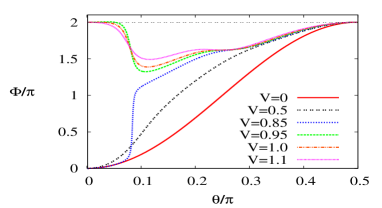
Figure 1: (color online). The geometric phase $\Phi=\Phi(\pi/\omega_{0})$ vs the mixing angle $\theta$ for the neutrino interacting with an ordinary matter for selected values of the dimensionless potential constant $V$ (the case of absence of dissipation, $C_{ij}=0$).

The main note is that in the absence of dissipation the GP does not depend on the Majorana angle $\phi$ and therefore the GP cannot be a tool for solving the Dirac vs Majorana neutrino dilemma. In Fig. 1 we illustrate details of the influence of the neutrino-matter interaction on the GP at time $t=\pi/\omega_{0}$, i.e. $\Phi(\pi/\omega_{0})$. With the increase of the neutrino energy $E$, the potential $V$ rises and at $V\approx 0.87$ the GP becomes a non–monotonic function of the mixing angle $\theta$, being significantly modified for $\theta$ smaller values. Yet with further increase of $V$ the GP as the function of $\theta$ stabilizes in the variation of $V$ and still at $V\approx 1.2$, i.e. when $\Delta^{2}m_{21}$ is active, it hardly feels the effect of further change of the neutrino energy, see Fig. 1. Let us notice that at one period trip $t=\pi/\omega_{0}$ and both $\theta$ and $\Delta^{2}m_{21}$ equal to the experimental solar neutrino values $\theta_{\odot}=0.188\,\pi$ and $\Delta^{2}m_{21}=8.0\times 10^{-5}$ ${\rm eV}^{2}$, respectively Giunti-Kim , the phase difference $\Phi(\pi/\omega_{0})-\Phi_{0}$ becomes approximately equal to the geometric value $\pi$ for $V\sim 1$ that means for the solar neutrino energies. Yet in the presence of ordinary matter the neutrino evolution is no more strictly cyclic at $t=\pi/\omega_{0}$ but at $t=\pi/\Omega$. One can attempt to quantify to what extent the cyclic character of the evolution is affected by the interaction with an ordinary matter in terms of the trace distance between the state at $t=\pi/\omega_{0}$ and the initial state nielsen :

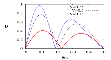
Figure 2: (color online). The trace distance $D$ calculated as in Eq.(20) plotted vs the mixing angle $\theta$ for different values of $V$. Remaining parameters are as in Fig. 1.

$$D=\frac{1}{2}||\rho(t=0)-\rho(t=\pi/\omega_{0})||\,,$$ (20)

where the norm $||\varrho||=\mbox{Tr}\sqrt{\varrho^{\dagger}\varrho}$. For a cyclic evolution, when the final and initial wave functions differ up to an overall phase factor, $D=0$. As seen from Fig. 2, the departure from the cyclic evolution quantified by $D$ is strongly affected by the mixing angle and, for certain angles the evolution, despite the presence of an ordinary matter ($V\neq 0$) remains cyclic, and this happens for $V\sim~{}1$ at the solar experimental value $\theta=0.188\,\pi$ again. It is interesting to analyze how the GP depends on choice of the time $t$. We have compared $\Phi(\pi/\omega_{0})$ and $\Phi(\pi/\Omega)$ for the mixing angle corresponding to the solar neutrino value $\theta=0.188\,\pi$. For $V\in[0,1.2]$, the difference $\Phi(\pi/\Omega)-\Phi(\pi/\omega_{0})$ is extremely small and from the experimental point of view negligible.

When the quantum system interacts with an environment, properties of the GP can be radically modified my . In the presence of dissipation, when the dissipation matrix $C_{ij}$ in Eq.(11) is not identically zero, the GP can be determined by solving Eq. (10) with (11) using, e.g. the Bloch vector formalism Bloch to obtain the coupled evolution equations for mean values $\langle\sigma_{k}(t)\rangle,k=x,y,z$. Next, the reduced density matrix is found as $\rho(t)=(1/2)[1+\langle\sigma_{x}(t)\rangle\sigma_{x}+\langle\sigma_{y}(t)\rangle\sigma_{y}+\langle\sigma_{z}(t)\rangle\sigma_{z}]$. From this form one can obtain the spectral decomposition (12) and the phase $\Phi^{\alpha}(t)$. Such an analytical form of the GP is, however, rather cumbersome without exhibiting much physical insight. Therefore, we present here the numerical results for the GP. The analysis has shown that none of the features of the GP is affected by the dissipative effects given by the diagonal matrix $C_{ij}\sim\delta_{ij}$. Hence all the results presented so far hold true for quite a general class of dissipative effects. It does not mean that the dynamics of neutrinos is unaffected by environmental noise as in the diagonal case the trace distance $D$ in Eq.(20) approaches constant value $D\approx 1/2$ with no regard to any choice of an initial preparation. It is no more the case when there is an off–diagonal contribution to the dissipation matrix $C_{ij}$. In Fig. 3 we present how the dissipation can affect the GP provided that there are nonvanishing off–diagonal elements in $C_{ij}$. The significant impact of dissipation is present only in a relatively narrow range of mixing angle $\theta$. Additionally, there is a feature which makes an off–diagonal dissipation worth studying: there is a nontrivial $\phi$–dependence of the GP. In Fig. 3 the considerations are limited to a single nonvanishing element $C(1,2)=C(2,1)=1/10$ and for the solar neutrino mixing angle $\theta=0.188\pi=33.9^{\circ}$. The results of other calculations, not reproduced here, show that the presented behavior is qualitatively generic. A most intriguing behavior on the role of the Majorana angle emerges when the angle $\phi$ is allowed to vary and the mixing angle $\theta$ is fixed. One can observe that the GP does depend on the Majorana angle $\phi$ in a non-monotonic way and is always minimal for the Dirac neutrino; for the Majorana neutrino the GP is greater than for the Dirac neutrino. This property of the GP can provide a significant test for the type of neutrino, the Majorana or Dirac one. Let us notice that this effect originates essentially from the dissipative character of an evolution since it is also present for the case $V=0$. Since dissipation is a generic feature of the quantum world, the $\phi$–dependence of the geometric phase seems to be generic as well.

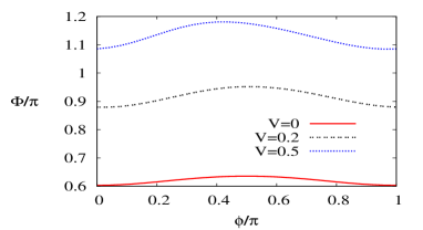
Figure 3: (color online). The geometric phase $\Phi=\Phi(\pi/\omega_{0})$ vs the Majorana angle $\phi$ in the presence of dissipation, $C(1,1)=C(2,2)=C(3,3)=1$, the off–diagonal contribution $C(1,2)=C(2,1)=1/10$ and for several values of $V$. The solar neutrino mixing angle is $\theta=0.188\pi=33.9^{\circ}$ Giunti-Kim .

In summary, the results reported in this paper show that the GP can be a potentially useful indicator of various properties of neutrinos and their environment. In the dissipationless case, the GP does not depend on the Majorana angle. However, in the presence of dissipation it is not the case anymore: the GP does depend on the Majorana angle and therefore can serve as a tool for determining the nature of the Dirac vs the Majorana neutrino. The theoretical analysis presented in the paper suggesting potential usefulness of the GP as a tool for distinguishing neutrino type achieves a real status of being useful provided that one can perform an experiment measuring the GP in neutrino oscillations. Any proposal of such an experiment, which requires highly sophisticated experimental methods even in the case on NMR-type systems fazmeasure , is beyond the scope of this brief report.

This work was supported by the MNiSW under Grant No. N202 064936.

References

- (1) E. Lisi et al., Phys. Rev. Lett. 85, 1166 (2000).
- (2) F.Benatti and R. Floreanini, Phys. Rev. D 64, 085015 (2001).
- (3) P. Mehta, Phys. Rev. D 79, 096013 (2009).
- (4) T.D. Gutierrez, Phys. Rev. Lett. 96, 121802 (2006).
- (5) S.M. Bilenky et al., Phys. Lett. 94B, 495 (1980); M. Doi et al., Phys. Lett. 102B, 323 (1981).
- (6) F. del Aguila et al., Phys. Rev. D 76, 013007 (2007).
- (7) X.–B. Wang et al., Phys. Rev. D 63, 053003 (2001); X.–G. He et al., Phys. Rev. D 72, 053012 (2005).
- (8) M. Blasone et al., Europhys. Lett. 85, 50002 (2009).
- (9) C. Giunti and C. W. Kim, Fundamentals of Neutrino Physics and Astrophysics (Oxford University Press, Oxford, 2007); B. Aharmim et al., Phys. Rev. C 72, 055502 (2005).
- (10) R. Alicki and K. Lendi, Quantum Dynamical Semigroups and Applications (Springer, Berlin, 1987).
- (11) F. Benatti and R. Floreanini, J. High Energy Phys. 2 (2000) 032 .
- (12) F. Benatti and R. Floreanini, Nucl. Phys. B488, 335 (1997); Nucl. Phys. B511, 550 (1998).
- (13) A. Uhlmann, Rep. Math. Phys. 9, 273 (1976).
- (14) A. Bassi and E. Ippoliti, Phys. Rev. A 73, 062104 (2006); N. Burić and M. Radonjić, Phys. Rev. A 80, 014101 (2009).
- (15) E. Sjöqvist et al., Phys. Rev. Lett. 85, 2845 (2000); R. Bhandari, Phys. Rev. Lett. 89, 268901 (2002); E. Sjöqvist, Phys. Rev. A 70, 052109 (2004); R. Bhandari, Phys. Rep. 281, 1 (1997); J. Du et al., Phys. Rev. Lett. 91, 100403 (2003).
- (16) D. M. Tong et al., Phys. Rev. Lett. 93, 080405 (2004).
- (17) F. M. Cucchietti et al., Phys. Rev. Lett. 105, 240406 (2010).
- (18) D. Chruściński and A. Jamiołkowski,Geometric Phases in Classical and Quantum Mechanics, (Birkhauser, Boston, 2004).
- (19) M. A. Nielsen and L. I. Chuang, Quantum Computation and Quantum Information (Cambridge University Press, Cambridge, 2000).
- (20) J. Dajka et al., J. Phys. A 41, 012001 (2008); J. Phys. A 41, 442001 (2008); Quant. Info. Proc. 10, 85 (2011).
- (21) V. Gorini et al., J. Math. Phys. (N.Y.) 17, 821 (1976).