Linearized FE approximations to a strongly nonlinear diffusion equation

Abstract

We study fully discrete linearized Galerkin finite element approximations to a nonlinear gradient flow, applications of which can be found in many areas. Due to the strong nonlinearity of the equation, existing analyses for implicit schemes require certain restrictions on the time step and no analysis has been explored for linearized schemes. This paper focuses on the unconditionally optimal $L^{2}$ error estimate of a linearized scheme. The key to our analysis is an iterated sequence of time-discrete elliptic equations and a rigorous analysis of its solution. We prove the $W^{1,\infty}$ boundedness of the solution of the time-discrete system and the corresponding finite element solution, based on a more precise estimate of elliptic PDEs in $W^{2,2+\epsilon_{1}}$ and $H^{2+\epsilon_{2}}$ and a physical feature of the gradient-dependent diffusion coefficient. Numerical examples are provided to support our theoretical analysis.

Keywords: finite element, nonlinear diffusion, gradient flow, stability, error estimate

AMS subject classifications: 65N12, 65N30, 35K61.

1 Introduction

We consider the nonlinear diffusion equation

$$\frac{\partial u}{\partial t}-\nabla\cdot(\sigma(|\nabla u|^{2})\nabla u)=g$$ (1.1)

in a convex polygonal domain $\Omega$ in $\mathbb{R}^{2}$ with the Neumman boundary condition

$$\begin{array}[]{ll}\nabla u\cdot{\vec{n}}=0{}{}&\mbox{on}~{}~{}\partial\Omega\end{array}$$ (1.3)

and the initial condition

$$\begin{array}[]{ll}u(x,0)=u_{0}(x){}{}&\mbox{for}~{}~{}x\in\Omega,\end{array}$$ (1.5)

where $g$ is a given function and

$$\sigma(s^{2})=\frac{1}{\sqrt{\lambda^{2}+s^{2}}}$$ (1.6)

is a gradient-dependent diffusion coefficient, where $\lambda$ is a positive constant. The equation has been involved in many applications, such as minimal surface flow [29], prescribed mean curvature flow [16, 23], geometric measure theory [4], and a regularized model in image denoising [11, 13, 14, 19, 24, 30, 31, 34, 36]. A review article for the applications in image processing was given in [10].

Mathematical analysis of the nonlinear diffusion equation (1.1) was studied in [21, 23]. In particular, the $W^{1,\infty}$ regularity of the solution was proved in [21], which implies arbitrarily higher regularity of the solution in a smooth domain (by the method of Section 8.3.2 of [18]). Numerical methods and simulations for the nonlinear diffusion equation have been investigated extensively in the last several dacades. For examples, see [2, 31, 30, 36] for finite difference methods and [13, 16, 17, 19, 20, 21, 22] for finite element methods (FEMs). Explicit schemes may not be efficient due to their strong time-step restrictions. A fully implicit backward Euler–Galerkin FEM was analyzed in [21], where optimal convergence rate was proved under the condition $\tau=O(h^{2})$. Suboptimal error estimates for the scheme were presented in [22] under a weaker mesh restriction $\tau=o(h^{1/2})$, and further analysis on the convergence rate of the scheme with respect to the regularization parameter was given in [20]. The implicit backward Euler scheme was also studied in [19] with a lumped mass FEM, where $L^{\infty}$-boundedness of the numerical solution was proved and no error estimates were presented. In these fully implicit schemes, one has to solve a system of nonlinear equations at each time step and an extra inner iteration is needed. In addition to the implicit schemes, linearized semi-implicit FEMs for the nonlinear diffusion equation have also been investigated by several authors [13, 30, 33]. In this method, the gradient-dependent diffusion coefficient is calculated with the numerical solution at the last time step and Galerkin FEMs are used to solve the linearized equation. The scheme only requires the solution of a linear system at each time step, which is simple and efficient for implementation. However, theoretical error analysis of the linearized scheme seems very difficult due to the strong nonlinear structure. As far as we know, no optimal error estimates of linearized semi-implicit FEMs are available for the nonlinear diffusion equation. The major difficulty for the analysis of the semi-implicit scheme is due to the nature of the linearization of the scheme, which leads to the arising of the energy-norm errors at two different time levels in the error equation (see (3.23)-(3.26) for the estimates of the error equation).

In this paper, we study linearized backward Euler–Galerkin methods for the nonlinear system (1.1)-(1.5). Our focus is on unconditionally optimal error estimates of numerical methods. The key issue in the analysis is to establish the $W^{1,\infty}$ convergence of the numerical solution. To deal with the strong nonlinearity from the gradient-dependent diffusion coefficient, we introduce an iterated sequence of time-discrete elliptic PDEs as in [27, 28]. Thus the linearized backward Euler–Galerkin method coincides with the corresponding FE approximation to the time-discrete system. We prove the $W^{1,\infty}$ convergence of the solution of the time-discrete system and FE solution, in terms of a more precise estimate for elliptic PDEs in $W^{2,2+\epsilon_{1}}$ and $H^{2+\epsilon_{2}}$:

$$\|u\|_{L^{2+\epsilon_{1}}}\leq(1+\epsilon^{*}_{1})\|\Delta u\|_{L^{2+\epsilon_{1}}}$$

$$\|u\|_{H^{2+\epsilon_{2}}}\leq(1+\epsilon^{*}_{2})\|\Delta u\|_{H^{\epsilon_{2}}}\,,$$

and a physical feature of the gradient-dependent diffusion coefficient: $2|\sigma^{\prime}(s^{2})|s^{2}<\sigma(s^{2})$. With these a priori estimates, we establish the $L^{2}$-norm optimal error estimate without any time-step restrictions.

The rest part of this paper is organized as follows. In Section 2, we introduce some notations and the linearized backward Euler–Galerkin FEM for the nonlinear diffusion equation (1.1)-(1.5), and then we present our main results and our methodology. In Section 3, we prove our main results based on the regularity and $W^{1,\infty}$-convergence of the time-discrete solution, while the rigorous proof of the regularity and $W^{1,\infty}$-convergence of the time-discrete solution is postponed to Section 4. Numerical examples are presented in Section 5, which confirm our theoretical analysis and show clearly that the linearized scheme is efficient and no time-step conditions are needed.

2 Notations and main results

Let $\Omega$ be a given convex polygon in $\mathbb{R}^{2}$. For $1\leq p\leq\infty$ and any nonnegative integer $k$, we denote by $W^{k,p}(\Omega)$ the usual Sobolev space of functions defined on $\Omega$ and, to simplify the notations, we set $W^{k,p}:=W^{k,p}(\Omega)$, $H^{k}:=W^{k,2}(\Omega)$ and $L^{p}:=W^{0,p}$. For $s\in(0,1)$, we define $H^{k+s}:=(H^{k},H^{k+1})_{[s]}$ as the complex interpolation space between $H^{k}$ and $H^{k+1}$. More detailed discussions for the complex interpolation spaces can be found in literature, $e.g.$, see the classical book [5] by Bergh and Löfström.

For a given quasi-uniform triangulation of $\Omega$ into triangles $T_{j}$, $j=1,\cdots,J$, we denote by $h=\max_{1\leq j\leq J}\{\mbox{diam}\,T_{j}\}$ the mesh size and define a finite element space by

$$V_{h}^{r}=\{v_{h}\in C(\overline{\Omega}):v_{h}|_{T_{j}}\mbox{~{}is~{}a~{}polynomial of degree $r$}\}$$

so that $V_{h}^{r}$ is a subspace of $H^{1}(\Omega)$. Let $\Pi_{h}:C(\overline{\Omega})\rightarrow V_{h}^{r}$ denote the Lagrangian interpolation operator. Let $0=t_{0}<t_{1}<\cdots<t_{N}=T$ be a uniform partition of the time interval $[0,T]$ with $t_{n}=n\tau$. For a sequence of functions $\{f^{n}\}_{n=0}^{N}$, we define a time-difference operator by

$$D_{\tau}f^{n+1}=\frac{f^{n+1}-f^{n}}{\tau},\quad\mbox{for $n=0,1,\cdots,N-1$.}$$ (2.1)

We define the linearized backward Euler–Galerkin finite element scheme by

$$\big{(}D_{\tau}U^{n+1}_{h},v\big{)}+\big{(}\sigma(|\nabla U^{n}_{h}|^{2})\nabla U^{n+1}_{h},\nabla v\big{)}=\big{(}g^{n+1},v\big{)},\quad\forall v\in V_{h}^{r},$$ (2.2)

with the initial condition $U^{0}_{h}=\Pi_{h}u_{0}$ and $r\geq 2$. At each time step, the scheme only requires the solution of a linear system. Also we assume that the solution of (1.1)-(1.5) exists and satisfies

$$\|u_{0}\|_{H^{r+1}}+\|u\|_{L^{\infty}((0,T);H^{r+1})}+\|\partial_{t}u\|_{L^{\infty}((0,T);H^{r+1})}+\|\partial_{tt}u\|_{L^{2}((0,T);L^{2})}\leq M_{0},$$ (2.3)

where $M_{0}$ is some positive constant. For simplicity, we assume that $g=g(x,t)$ in this paper. The analysis presented in this paper can be easily extended to the general case $g=g(u,x,t)$ for the scheme

$$\big{(}D_{\tau}U^{n+1}_{h},v\big{)}+\big{(}\sigma(|\nabla U^{n}_{h}|^{2})\nabla U^{n+1}_{h},\nabla v\big{)}=\big{(}g(U^{n}_{h},x,t^{n}),v\big{)},\quad\forall v\in V_{h}^{r},$$

if $g$ is a smooth function of $u$, $x$ and $t$.

Our main results are given in the following theorem concerning the unconditionally optimal convergence rate of the numerical solution.

Theorem 2.1

Suppose that the system (1.1)-(1.5) has a unique solution $u$ satisfying the regularity condition (2.3). Then there exists a positive constant $C_{0}$, independent of $\tau$ and $h$, such that the finite element system (2.2) admits a unique solution $\{U^{n}_{h}\}_{n=1}^{N}$ satisfying

$$\|U_{h}^{n}-u^{n}\|_{L^{2}}\leq C_{0}(\tau+h^{r+1}).$$ (2.4)

To prove the above theorem, we introduce an iterated sequence of elliptic PDEs (time-discrete system) as proposed in [27, 28]:

$$D_{\tau}U^{n+1}-\nabla\cdot(\sigma(|\nabla U^{n}|^{2})\nabla U^{n+1})=g^{n+1},$$ (2.5)

with the boundary condition $\nabla U^{n+1}\cdot{\vec{n}}=0$ on $\partial\Omega$ and the initial condition $U^{0}=u_{0}$. Then the fully discrete solution $U^{n+1}_{h}$ coincides with the finite element solution of (2.5). In view of this property, we split the error into

$$U^{n}_{h}-u^{n}=(U^{n}_{h}-U^{n})+(U^{n}-u^{n})$$

and analyze the two error functions separately. The regularity of the solution of the time-discrete system (2.5) is given in the following theorem.

Theorem 2.2

Under the assumption of Theorem 2.1, there exist positive constants $\tau_{0}^{*}$, $C_{0}^{*}$, $p>2$ and $s_{0}>0$, which are dependent only on $M_{0}$, $\Omega$ and $T$ and independent of $\tau$ and $h$, such that when $\tau<\tau_{0}^{*}$ the time-discrete system (2.5) admits a unique solution $\{U^{n}\}_{n=0}^{N}$ satisfying

$$\max_{0\leq n\leq N}(\|U^{n}\|_{W^{2,p}}^{2}+\|U^{n}\|_{H^{2+s_{0}}}^{2})+\sum_{n=1}^{N}\tau\|D_{\tau}U^{n}\|_{H^{2}}^{2}\leq C_{0}^{*},$$ (2.6)

$$\max_{1\leq n\leq N}\|e^{n}\|_{H^{1}}^{2}+\sum_{n=1}^{N}\tau\|e^{n}\|_{H^{2}}^{2}+\sum_{n=1}^{N}\tau\|D_{\tau}e^{n}\|_{L^{2}}^{2}\leq C_{0}^{*}\tau^{2},$$ (2.7)

$$\max_{1\leq n\leq N}\|e^{n}\|_{W^{2,p}}\leq C_{0}^{*}\tau^{1/3},$$ (2.8)

where $e^{n}:=u^{n}-U^{n}$.

The proofs of Theorem 2.1 and Theorem 2.2 will be given in Section 3 and Section 4, respectively. In the rest part of this paper, we denote by $C$ a generic positive constant which is independent of $\tau$, $h$ and $n$, and by $\epsilon$ a generic small positive constant.

3 Proof of Theorem 2.1

In this section, we prove Theorem 2.1 based on the results of Theorem 2.2. The proof of the latter is deferred to Section 4. The following inverse inequalities will be used in this section:

$$\|v\|_{L^{p}}\leq Ch^{2/p-2/q}\|v\|_{L^{q}},~{}\qquad\quad\mbox{for}~{}~{}~{}v\in V_{h}^{r},~{}~{}\,1\leq q\leq p\leq\infty,$$ (3.1)

$$\|\nabla v\|_{L^{p}}\leq Ch^{-1}\|v\|_{L^{p}},~{}\qquad\qquad\mbox{for}~{}~{}~{}v\in V_{h}^{r},~{}~{}\,1\leq p\leq\infty.$$ (3.2)

3.1 Preliminaries

Based on Theorem 2.2, we define

$$M=\sup_{\tau}\max_{1\leq n\leq N}(\|u^{n}\|_{W^{1,\infty}}+\|U^{n}\|_{W^{1,\infty}})+1$$

so that

$$\sigma(|\nabla u^{n}|^{2})\geq\sigma_{M},\,\quad|\sigma(|\nabla u^{n}|^{2})|+|\sigma^{\prime}(|\nabla u^{n}|^{2})|+|\sigma^{\prime\prime}(|\nabla u^{n}|^{2})|\leq C_{M},$$

$$\sigma(|\nabla U^{n}|^{2})\geq\sigma_{M},\quad|\sigma(|\nabla U^{n}|^{2})|+|\sigma^{\prime}(|\nabla U^{n}|^{2})|+|\sigma^{\prime\prime}(|\nabla U^{n}|^{2})|\leq C_{M},$$

for some positive constants $\sigma_{M}$ and $C_{M}$.

For any given function $w\in H^{1}$, we define the following matrix functions:

$$B(\nabla w)=2\sigma^{\prime}(|\nabla w|^{2})\nabla w(\nabla w)^{T}\,,\qquad A(\nabla w)=\sigma(|\nabla w|^{2})I+B(\nabla w)\,.$$ (3.3)

For $n\geq 0$ we define the projection operators $\overline{R}_{h}^{n+1}:H^{1}(\Omega)\rightarrow V_{h}^{r}$ and $R_{h}^{n+1}:H^{1}(\Omega)\rightarrow V_{h}^{r}$ by

$$\big{(}A(\nabla u^{n})\nabla(w-\overline{R}_{h}^{n+1}w),\nabla v\big{)}=0,\quad\forall~{}~{}w\in H^{1}~{}~{}\mbox{and}~{}~{}v\in V_{h}^{r},$$ (3.4)

$$\big{(}A(\nabla U^{n})\nabla(w-R_{h}^{n+1}w),\nabla v\big{)}=0,\quad\forall~{}~{}w\in H^{1}~{}~{}\mbox{and}~{}~{}v\in V_{h}^{r},$$ (3.5)

where $\int_{\Omega}\overline{R}_{h}^{n+1}w{\rm d}x=\int_{\Omega}R_{h}^{n+1}w{\rm d}x=\int_{\Omega}w{\rm d}x$ are enforced for uniqueness, and we set $\overline{R}_{h}^{0}:=\overline{R}_{h}^{1}$, $R_{h}^{0}:=R_{h}^{1}$. These two projection operators are well defined since

$$\lambda^{2}\sigma_{M}^{3}|\xi|^{2}\leq\xi^{T}A(\nabla u^{n})\xi\leq 2C_{M}|\xi|^{2},\quad\,\forall~{}\xi\in\mathbb{R}^{2}\,,$$

$$\lambda^{2}\sigma_{M}^{3}|\xi|^{2}\leq\xi^{T}A(\nabla U^{n})\xi\leq 2C_{M}|\xi|^{2},\quad\forall~{}\xi\in\mathbb{R}^{2}\,.$$

We denote

$$\theta^{n+1}_{h}=U^{n+1}-R_{h}^{n+1}U^{n+1},\quad\mbox{ and }\quad\overline{\theta}^{n+1}_{h}=u^{n+1}-\overline{R}_{h}^{n+1}u^{n+1}\,.$$

By the classical theory of finite element methods, with the regularity of $U^{n}$ given in Theorem 2.2, we have

$$\|u^{n+1}-R_{h}^{n+1}u^{n+1}\|_{W^{1,\infty}}\leq C\|u^{n+1}\|_{H^{3}}h,$$ (3.6)

$$\|\overline{\theta}^{n+1}_{h}\|_{H^{l}}\leq C\|u^{n+1}\|_{H^{r+1}}h^{r+1-l},\qquad\mbox{for}~{}~{}l=0,1,$$ (3.7)

$$\|R_{h}^{n+1}U^{n+1}\|_{W^{1,\infty}}+\|\overline{R}_{h}^{n+1}u^{n+1}\|_{W^{1,\infty}}\leq C(\|U^{n+1}\|_{W^{1,\infty}}+\|u^{n+1}\|_{W^{1,\infty}}),$$ (3.8)

$$\|\tau D_{\tau}\nabla U^{n+1}\|_{L^{\infty}}\leq C\|\tau D_{\tau}\nabla e^{n+1}\|_{L^{\infty}}+C\|\tau D_{\tau}\nabla u^{n+1}\|_{L^{\infty}}\leq C\tau^{1/3},$$ (3.9)

$$\|D_{\tau}A(\nabla U^{n})\|_{L^{\bar{p}}}\leq C\|D_{\tau}\nabla U^{n}\|_{L^{\bar{p}}}\leq C\|D_{\tau}U^{n}\|_{H^{2}},$$ (3.10)

and

$$\|\theta^{n+1}_{h}\|_{W^{l,q}} \leq\|e^{n+1}-R_{h}^{n+1}e^{n+1}\|_{W^{l,q}}+\|u^{n+1}-R_{h}^{n+1}u^{n+1}\|_{W^{l,q}}$$

$$\leq Ch^{2-l}\|e^{n+1}\|_{W^{2,q}}+Ch^{2-l+2/q}\|u^{n+1}\|_{H^{3}}\quad\mbox{for $l=0,1$ and $2\leq q\leq p$},$$ (3.11)

where $p$ is given in Theorem 2.2 and $1/\bar{p}+1/p=1/2$. The above inequality (3.7) with $l=0,1$ is standard $L^{2}$ and $H^{1}$ error estimate of the finite element method for elliptic equations, respectively. Since $A(\nabla U^{n})\in W^{1,p}$ for some $p>2$, the $L^{2}$ error estimate $\|u^{n+1}-R_{h}^{n+1}u^{n+1}\|_{L^{2}}\leq Ch^{3}\|u^{n+1}\|_{H^{3}}$ is also standard. Then, (3.6) can be derived by introducing an extra interpolation and an inverse inequality (see page 93, of the book [7]. Moreover, (3.8) and (3.11) follow from Theorem 8.1.11 and Theorem 8.5.3 of [8], respectively, and (3.9)-(3.10) are consequences of Theorem 2.2. From these inequalities we also derive that

$$\|\theta^{n}_{h}\|_{W^{1,\infty}} \leq\|e^{n}-R_{h}^{n}e^{n}\|_{W^{1,\infty}}+\|u^{n}-R_{h}^{n}u^{n}\|_{W^{1,\infty}}$$

$$\leq C\|e^{n}\|_{W^{1,\infty}}+Ch\|u^{n}\|_{H^{3}}$$

$$\leq C(\tau^{1/3}+h).$$ (3.12)

In this section, we shall frequently use the inequalities (3.6)-(3.12). Moreover, we need the following Lemma.

Lemma 3.1

Under the assumptions of Theorem 2.1, there exist positive constants $\widetilde{\tau}_{0}$ and $\delta_{0}$ such that when $\tau\leq\widetilde{\tau}_{0}$,

$$\biggl{(}\sum_{n=0}^{N-1}\tau\|D_{\tau}\theta^{n+1}_{h}\|_{H^{-1}}^{2}\biggl{)}^{\frac{1}{2}}\leq C(\tau^{1/3}+h^{\delta_{0}})h^{2},$$ (3.13)

$$\biggl{(}\sum_{n=0}^{N-1}\tau\|D_{\tau}(u^{n+1}-R_{h}^{n+1}u^{n+1})\|_{H^{1}}^{2}\biggl{)}^{\frac{1}{2}}\leq Ch^{r},$$ (3.14)

$$\biggl{(}\sum_{n=0}^{N-1}\tau\|D_{\tau}\overline{\theta}^{n+1}_{h}\|_{L^{2}}^{2}\biggl{)}^{\frac{1}{2}}\leq Ch^{r+1}.$$ (3.15)

Proof   Since $u^{n}$ is smooth enough, (3.14)-(3.15) can be obtained easily. Here we only prove (3.13). Note that

$$\Big{(}A(\nabla U^{n})\nabla(U^{n+1}-R_{h}^{n+1}U^{n+1}),\,\nabla\phi_{h}\Big{)}=0,$$ (3.16)

$$\Big{(}A(\nabla U^{n-1})\nabla(U^{n+1}-R_{h}^{n}U^{n+1}),\,\nabla\phi_{h}\Big{)}=0.$$ (3.17)

The difference of the above two equations gives

$$\Big{(}A(\nabla u^{n})\nabla(R_{h}^{n}U^{n+1}-R_{h}^{n+1}U^{n+1}),\,\nabla\phi_{h}\Big{)}$$

$$+\Big{(}(A(\nabla U^{n})-A(\nabla u^{n}))\nabla(R_{h}^{n}U^{n+1}-R_{h}^{n+1}U^{n+1}),\,\nabla\phi_{h}\Big{)}$$

$$+\Big{(}(A(\nabla U^{n})-A(\nabla U^{n-1}))\nabla(U^{n+1}-R_{h}^{n}U^{n+1}),\,\nabla\phi_{h}\Big{)}=0,$$

which together with Theorem 2.2 implies

$$\|\nabla(R_{h}^{n}U^{n+1}-R_{h}^{n+1}U^{n+1})\|_{L^{2}}$$

$$\leq C\|(A(\nabla U^{n})-A(\nabla u^{n}))\nabla(R_{h}^{n}U^{n+1}-R_{h}^{n+1}U^{n+1})\|_{L^{2}}$$

$$~{}~{}~{}+C\|(A(\nabla U^{n})-A(\nabla U^{n-1}))\nabla(U^{n+1}-R_{h}^{n}U^{n+1})\|_{L^{2}}$$

$$\leq C\|\nabla e^{n}\|_{L^{\infty}}\|\nabla(R_{h}^{n}U^{n+1}-R_{h}^{n+1}U^{n+1})\|_{L^{2}}+C\tau\|D_{\tau}\nabla U^{n}\|_{L^{\bar{p}}}\|\nabla(U^{n+1}-R_{h}^{n}U^{n+1})\|_{L^{p}}$$

$$\leq C\tau^{1/3}\|\nabla(R_{h}^{n}U^{n+1}-R_{h}^{n+1}U^{n+1})\|_{L^{2}}$$

$$~{}~{}~{}+C\tau\|D_{\tau}U^{n}\|_{H^{2}}(\|e^{n+1}-R_{h}^{n}e^{n+1}\|_{W^{1,p}}+\|u^{n+1}-R_{h}^{n}u^{n+1}\|_{W^{1,p}})$$

$$\leq C\tau^{1/3}\|\nabla(R_{h}^{n}U^{n+1}-R_{h}^{n+1}U^{n+1})\|_{L^{2}}$$

$$~{}~{}~{}+C\tau\|D_{\tau}U^{n}\|_{H^{2}}(Ch\|e^{n+1}\|_{W^{2,p}}+Ch^{1+2/p}\|u^{n+1}\|_{H^{3}})$$

$$\leq C\tau^{1/3}\|\nabla(R_{h}^{n}U^{n+1}-R_{h}^{n+1}U^{n+1})\|_{L^{2}}+C\|D_{\tau}U^{n}\|_{H^{2}}(\tau^{1/3}+h^{2/p})\tau h,$$

where we have used (2.8), (3.10) and a similar $W^{1,p}$ estimate as given in (3.11). When $\tau<\widetilde{\tau}_{0}:=\min(\tau_{0}^{*},(2C)^{-3})$, we get

$$\|\nabla(R_{h}^{n}U^{n+1}-R_{h}^{n+1}U^{n+1})\|_{L^{2}} \leq 2C\|D_{\tau}U^{n}\|_{H^{2}}(\tau^{1/3}+h^{2/p})\tau h.$$ (3.18)

To establish the corresponding $L^{2}$-norm estimate, for any given $\varphi\in H^{1}(\Omega)$ we let $\psi$ be the solution of the equation

$$-\nabla\cdot\Big{(}A(\nabla U^{n})\nabla\psi\Big{)}=\varphi-\frac{1}{|\Omega|}\int_{\Omega}\varphi{\rm d}x$$

with the boundary condition $A(\nabla U^{n})\nabla\psi\cdot{\vec{n}}=0$ on $\partial\Omega$ and $\int_{\Omega}\psi{\rm d}x=0$. Due to the structure of the matrix $A(\nabla U^{n})$, this boundary condition is equivalent to $\nabla\psi\cdot{\vec{n}}=0$ on $\partial\Omega$. Since $A(\nabla U^{n})$ is uniformly bounded in $W^{1,p}\cap H^{1+s_{0}}$, there exists a positive constant $\delta_{0}\in(0,\min(2/p,s_{0}))$ (dependent on the norm $\|\nabla U^{n}\|_{H^{1+s_{0}}}$) such that $\|\psi\|_{H^{2+s}}\leq C\|\varphi\|_{H^{s}}$ for $s\in[0,\delta_{0}]$ (see Appendix).

By noting the fact that $\int_{\Omega}(R_{h}^{n}U^{n+1}-R_{h}^{n+1}U^{n+1}){\rm d}x=0$, we have

$$\big{(}R_{h}^{n}U^{n+1}-R_{h}^{n+1}U^{n+1},\varphi)$$

$$=\Big{(}A(\nabla U^{n})\nabla(R_{h}^{n}U^{n+1}-R_{h}^{n+1}U^{n+1}),\,\nabla\psi\Big{)}$$

$$=\Big{(}A(\nabla U^{n})\nabla(R_{h}^{n}U^{n+1}-R_{h}^{n+1}U^{n+1}),\,\nabla(\psi-\Pi_{h}\psi)\Big{)}$$

$$~{}~{}~{}-\Big{(}(A(\nabla U^{n})-A(\nabla U^{n-1}))\nabla(U^{n+1}-R_{h}^{n}U^{n+1}),\,\nabla(\Pi_{h}\psi-\psi)\Big{)}$$

$$~{}~{}~{}-\Big{(}(A(\nabla U^{n})-A(\nabla U^{n-1})\nabla(U^{n+1}-R_{h}^{n}U^{n+1}),\,\nabla\psi\Big{)}:=R_{1}+R_{2}+R_{3}$$

By (3.11) and (3.18), the first two terms of the right-hand side of the above equation are bounded by

$$|R_{1}| \leq C\|D_{\tau}U^{n}\|_{H^{2}}\|\psi\|_{H^{2}}(\tau^{1/3}+h^{2/p})\tau h^{2},$$

$$|R_{2}| \leq C\|D_{\tau}A(\nabla U^{n})\|_{L^{\bar{p}}}\|\nabla(U^{n+1}-R_{h}^{n}U^{n+1})\|_{L^{p}}\|\psi\|_{H^{2}}\tau h$$

$$\leq C\|D_{\tau}U^{n}\|_{H^{2}}\|\psi\|_{H^{2}}(\tau^{1/3}+h^{2/p})\tau h^{2},$$

where $1/\bar{p}+1/p=1/2$. Again by (2.8), (3.11) and (3.18) and noting the homogeneous boundary condition, with integration by part, we can bound the last term by

$$|R_{3}|=\Big{|}\Big{(}(A(\nabla U^{n})-A(\nabla U^{n-1}))\nabla(U^{n+1}-R_{h}^{n}U^{n+1}),\,\nabla\psi\Big{)}\Big{|}$$

$$=\Big{|}\Big{(}U^{n+1}-R_{h}^{n}U^{n+1},\nabla\cdot\big{[}(A(\nabla U^{n})-A(\nabla U^{n-1}))\nabla\psi\big{]}\Big{)}\Big{|}$$

$$\leq\|U^{n+1}-R_{h}^{n}U^{n+1}\|_{L^{p}}\|\nabla\cdot\big{[}(A(\nabla U^{n})-A(\nabla U^{n-1}))\nabla\psi\big{]}\|_{L^{p^{\prime}}}$$

$$\leq C(h^{2}\|e^{n+1}\|_{W^{2,p}}+h^{2+2/p}\|u^{n+1}\|_{H^{3}})\left(\|A(\nabla U^{n})-A(\nabla U^{n-1})\|_{H^{1}}\|\nabla\psi\|_{L^{\widetilde{p}}}\right.$$

$$~{}~{}~{}+\left.\|A(\nabla U^{n})-A(\nabla U^{n-1})\|_{L^{\widetilde{p}}}\|\psi\|_{H^{2}}\right)$$

$$\leq C\|D_{\tau}U^{n}\|_{H^{2}}\|\varphi\|_{L^{2}}(\tau^{1/3}+h^{2/p})\tau h^{2},$$

where $1/p+1/p^{\prime}=1$ and $1/\widetilde{p}+1/2=1/p^{\prime}$.

With the above estimates, we obtain

$$\|R_{h}^{n}U^{n+1}-R_{h}^{n+1}U^{n+1}\|_{L^{2}}\leq C\|D_{\tau}U^{n}\|_{H^{2}}(\tau^{1/3}+h^{2/p})\tau h^{2}\quad\mbox{for}~{}~{}n\geq 1.$$

Since $R_{h}^{0}U^{1}=R_{h}^{1}U^{1}$, we have

$$\biggl{(}\sum_{n=0}^{N-1}\tau\|R_{h}^{n}U^{n+1}-R_{h}^{n+1}U^{n+1}\|_{L^{2}}^{2}\biggl{)}^{\frac{1}{2}}\leq C(\tau^{1/3}+h^{2/p})\tau h^{2}.$$

Finally, we take a standard approach to the $H^{-1}$-norm estimate (3.13) [8]. Since

$$|(\phi-R_{h}\phi,\varphi)| =\inf_{\psi_{h}\in V_{h}^{r}}|(A(\nabla U^{n})\nabla(\phi-R_{h}\phi),\nabla(\psi-\psi_{h}))|$$

$$\leq C\|\nabla(\phi-R_{h}\phi)\|_{L^{2}}\|\psi\|_{H^{2+\delta_{0}}}h^{1+\delta_{0}}$$

$$\leq C\|\phi\|_{H^{2}}\|\varphi\|_{H^{\delta_{0}}}h^{2+\delta_{0}},\quad\forall~{}\varphi\in H^{\delta_{0}},$$

we have

$$\|\phi-R_{h}\phi\|_{H^{-\delta_{0}}}\leq C\|\phi\|_{H^{2}}h^{2+\delta_{0}},\quad\forall~{}\phi\in H^{2}$$

from which, we further derive that

$$\|D_{\tau}(U^{n+1}-R_{h}^{n+1}U^{n+1})\|_{H^{-1}}$$

$$\leq\|D_{\tau}U^{n+1}-R_{h}^{n}D_{\tau}U^{n+1}\|_{H^{-1}}+\tau^{-1}\|R_{h}^{n+1}U^{n+1}-R_{h}^{n}U^{n+1}\|_{H^{-1}}$$

$$\leq\|D_{\tau}U^{n+1}-R_{h}^{n}D_{\tau}U^{n+1}\|_{H^{-\delta_{0}}}+\tau^{-1}\|R_{h}^{n+1}U^{n+1}-R_{h}^{n}U^{n+1}\|_{L^{2}}$$

$$\leq C\|D_{\tau}e^{n+1}\|_{H^{2}}h^{2+\delta_{0}}+C\|D_{\tau}u^{n+1}\|_{H^{3}}h^{3}+\tau^{-1}\|R_{h}^{n+1}U^{n+1}-R_{h}^{n}U^{n+1}\|_{L^{2}}.$$

(3.13) follows immediately.   

3.2 Boundedness of the numerical solution

By (2.6) and (3.8), we can re-define

$$M =\sup_{\tau,h}\Big{(}\max_{0\leq n\leq N}\|u^{n}\|_{W^{1,\infty}}+\max_{0\leq n\leq N}\|\overline{R}_{h}^{n}u^{n}\|_{W^{1,\infty}}$$

$$~{}~{}~{}+\max_{0\leq n\leq N}\|U^{n}\|_{W^{1,\infty}}+\max_{0\leq n\leq N}\|R_{h}^{n}U^{n}\|_{W^{1,\infty}}\Big{)}+2.$$

By the regularity assumptions on $\sigma$, there exist $\sigma_{M}$ and $C_{M}>0$ such that

$$\sigma(s^{2})\geq\sigma_{M},\qquad\qquad\qquad\qquad\qquad\forall~{}s\in[-M,M],$$ (3.19)

$$|\sigma(s^{2})|+|\sigma^{\prime}(s^{2})|+|\sigma^{\prime\prime}(s^{2})|\leq C_{M},\quad~{}\forall~{}s\in[-M,M].$$ (3.20)

Lemma 3.2

Under the assumptions of Theorem 2.1, there exist positive constants $\widehat{\tau}_{0}$ and $\widehat{h}_{0}$ which are independent of $n$, $\tau$ and $h$, such that the finite element system (2.2) admits a unique solution $\{U^{n}_{h}\}_{n=1}^{N}$ when $\tau<\widehat{\tau}_{0}$ and $h<\widehat{h}_{0}$, satisfying

$$\|U_{h}^{n}\|_{L^{\infty}}+\|\nabla U_{h}^{n}\|_{L^{\infty}}\leq M,$$ (3.21)

$$\|e^{n}_{h}\|_{L^{\infty}}+\|\nabla e^{n}_{h}\|_{L^{\infty}}<\tau^{1/8}+h^{\delta_{0}/8},$$ (3.22)

where $e_{h}^{n}=R_{h}^{n}U^{n}-U^{n}_{h}$ and $\delta_{0}$ is given in Lemma 3.1.

Proof    By (3.19)-(3.20), the coefficient matrix of the linear system (2.2) is symmetric and positive definite, which implies that (2.2) admits a unique solution $U^{n+1}_{h}\in V_{h}^{r}$ for $0\leq n\leq k$.

It is easy to see that the inequalities (3.21)-(3.22) hold for $n=0$. By mathematical induction, we can assume that (3.21)-(3.22) hold for $0\leq n\leq k$ for some $k\geq 0$.

Since the solution $U^{n+1}$ of (2.5) satisfies

$$\big{(}D_{\tau}U^{n+1},v\big{)}+\big{(}\sigma(|\nabla U^{n}|^{2})\nabla U^{n+1},\nabla v\big{)}=\big{(}g^{n+1},v\big{)},\quad\forall~{}v\in V_{h}^{r},$$

the error function $e_{h}^{n+1}$ satisfies

$$\big{(}D_{\tau}e^{n+1}_{h},v\big{)}+\big{(}\sigma(|\nabla U^{n}|^{2})\nabla e^{n+1}_{h},\nabla v\big{)}$$ (3.23)

$$=\Big{[}-\big{(}\sigma(|\nabla U^{n}|^{2})\nabla\theta^{n+1}_{h},\,\nabla v\big{)}+\big{(}(\sigma(|\nabla U_{h}^{n}|^{2})-\sigma(|\nabla U^{n}|^{2}))\nabla U^{n+1}_{h},\nabla v\big{)}\Big{]}-\big{(}D_{\tau}\theta^{n+1}_{h},v\big{)}$$

$$:=J_{1}(v)+J_{2}(v),\qquad\forall~{}v\in V_{h}^{r}.$$

By using Taylor’s expansion, we see that

$$(\sigma(|\nabla U_{h}^{n}|^{2})-\sigma(|\nabla U^{n}|^{2}))\nabla U^{n+1}_{h}$$

$$=\left(2\sigma^{\prime}(|\nabla U^{n}|^{2})\nabla U^{n}\cdot\nabla(U_{h}^{n}-U^{n})+\sigma^{\prime}(|\nabla U^{n}|^{2})|\nabla(U_{h}^{n}-U^{n})|^{2}\right)\nabla U^{n+1}$$

$$~{}~{}~{}+\frac{1}{2}\sigma^{\prime\prime}(\xi^{n}_{h})|\nabla(U_{h}^{n}+U^{n})\cdot\nabla(U_{h}^{n}-U^{n})|^{2}\nabla U^{n+1}$$

$$~{}~{}~{}+(\sigma(|\nabla U_{h}^{n}|^{2})-\sigma(|\nabla U^{n}|^{2}))\nabla(-e^{n+1}_{h}-\theta^{n+1}_{h})$$

$$=-2\sigma^{\prime}(|\nabla U^{n}|^{2})\nabla U^{n}\cdot\nabla(e^{n}_{h}+\theta^{n+1}_{h})(\nabla U^{n}+\tau D_{\tau}\nabla U^{n+1})$$

$$~{}~{}~{}+2\sigma^{\prime}(|\nabla U^{n}|^{2})\nabla U^{n}\cdot\nabla\tau D_{\tau}\theta^{n+1}_{h}\nabla U^{n+1}$$

$$~{}~{}~{}+\Big{(}\sigma^{\prime}(|\nabla U^{n}|^{2})|\nabla(U_{h}^{n}-U^{n})|^{2}+\frac{1}{2}\sigma^{\prime\prime}(\xi^{n}_{h})|\nabla(U^{n}+U_{h}^{n})\cdot\nabla(e^{n}_{h}+\theta^{n}_{h})|^{2}\Big{)}\nabla U^{n+1}$$

$$~{}~{}~{}-(\sigma(|\nabla U_{h}^{n}|^{2})-\sigma(|\nabla U^{n}|^{2}))\nabla(e^{n+1}_{h}+\theta^{n+1}_{h})$$ (3.24)

where $\xi_{h}^{n}$ is some number between $|\nabla U_{h}^{n}|^{2}$ and $|\nabla U^{n}|^{2}$. By using the notations in (3.3), we see further that

$$J_{1}(v) =-\big{(}A(\nabla U^{n})\nabla\theta^{n+1}_{h},\,\nabla v\big{)}$$

$$~{}~{}~{}-\big{(}2\sigma^{\prime}(|\nabla U^{n}|^{2})\nabla U^{n}\cdot\nabla\theta^{n+1}_{h}\tau D_{\tau}\nabla U^{n+1},\,\nabla v\big{)}$$

$$~{}~{}~{}-\big{(}2\sigma^{\prime}(|\nabla U^{n}|^{2})(\nabla U^{n}\cdot\nabla e^{n}_{h})\nabla U^{n+1},\,\nabla v\big{)}$$

$$~{}~{}~{}+\big{(}2\sigma^{\prime}(|\nabla U^{n}|^{2})\nabla U^{n}\cdot\nabla\tau D_{\tau}\theta^{n+1}_{h}\nabla U^{n+1},\,\nabla v\big{)}$$

$$~{}~{}~{}+\big{(}\sigma^{\prime}(|\nabla U^{n}|^{2})|\nabla(U_{h}^{n}-U^{n})|^{2}+\frac{1}{2}\sigma^{\prime\prime}(\xi^{n}_{h})|\nabla(U^{n}+U_{h}^{n})\cdot\nabla(e^{n}_{h}+\theta^{n}_{h})|^{2}\nabla U^{n+1},\,\nabla v\big{)}$$

$$~{}~{}~{}-\big{(}(\sigma(|\nabla U_{h}^{n}|^{2})-\sigma(|\nabla U^{n}|^{2}))\nabla(e^{n+1}_{h}+\theta^{n+1}_{h}),\,\nabla v\big{)}.$$

Let

$$\gamma(|\nabla U^{n}|^{2})=2|\sigma^{\prime}(|\nabla U^{n}|^{2})||\nabla U^{n}|^{2}=\sigma(|\nabla U^{n}|^{2})-\lambda^{2}\sigma(|\nabla U^{n}|^{2})^{3}.$$ (3.25)

Taking $v=e_{h}^{n+1}$ in (3.23) and noting the fact $\big{(}A(\nabla U^{n})\nabla\theta^{n+1}_{h},\,\nabla e_{h}^{n+1}\big{)}=0$, we obtain

$$J_{1}(e_{h}^{n+1}) \leq\big{(}\gamma(|\nabla U^{n}|^{2})|\nabla e_{h}^{n+1}|,|\nabla e_{h}^{n}|\big{)}$$

$$~{}~{}~{}+C\|\tau D_{\tau}\nabla U^{n+1}\|_{L^{\infty}}(\|\nabla e_{h}^{n}\|_{L^{2}}+\|\nabla\theta^{n+1}_{h}\|_{L^{2}})\|\nabla e_{h}^{n+1}\|_{L^{2}}$$

$$~{}~{}~{}+C\biggl{(}\sum_{m=n}^{n+1}\|e^{m}-R_{h}^{m}e^{m}\|_{H^{1}}+\tau\|D_{\tau}(u^{n+1}-R_{h}^{n+1}u^{n+1})\|_{H^{1}}\biggl{)}\|\nabla e_{h}^{n+1}\|_{L^{2}}$$

$$~{}~{}~{}+C(\|\nabla e_{h}^{n}\|_{L^{\infty}}+\|\nabla\theta^{n}_{h}\|_{L^{\infty}})(\|\nabla e_{h}^{n}\|_{L^{2}}+\|\nabla\theta^{n}_{h}\|_{L^{2}})\|\nabla e_{h}^{n+1}\|_{L^{2}}$$

$$~{}~{}~{}+C(\|\nabla e_{h}^{n}\|_{L^{\infty}}+\|\nabla\theta^{n}_{h}\|_{L^{\infty}})(\|\nabla\theta^{n+1}_{h}\|_{L^{2}}\|\nabla e_{h}^{n+1}\|_{L^{2}}+\|\nabla e_{h}^{n+1}\|_{L^{2}}^{2}).$$

From (3.11), (3.12) and (3.22) we have

$$\|\nabla\theta^{n}_{h}\|_{L^{2}}\leq Ch\|e^{n}\|_{H^{2}}+Ch^{2},$$

$$\|\nabla e_{h}^{n}\|_{L^{\infty}}+\|\nabla\theta^{n}_{h}\|_{L^{\infty}}\leq C(\tau^{1/8}+h^{\delta_{0}/8})<\epsilon$$

when $\tau<\tau_{1}$ and $h<h_{1}$ for some positive constants $\tau_{1}$ and $h_{1}$ (which depend on the constant $\epsilon$). With (3.6)-(3.12), the induction assumptions (3.21)-(3.22) and the regularity of $U^{n}$ given in Theorem 2.2, we derive that,

$$J_{1}(e_{h}^{n+1}) \leq\frac{1}{2}\Big{\|}\sqrt{\gamma(|\nabla U^{n}|^{2})}\nabla e_{h}^{n+1}\Big{\|}_{L^{2}}^{2}+\frac{1}{2}\Big{\|}\sqrt{\gamma(|\nabla U^{n}|^{2})}\nabla e_{h}^{n}\Big{\|}_{L^{2}}^{2}+C\tau^{1/3}\|\nabla e_{h}^{n}\|_{L^{2}}\|\nabla e_{h}^{n+1}\|_{L^{2}}$$

$$~{}~{}~{}+C(h\|e^{n+1}\|_{H^{2}}+h\|e^{n}\|_{H^{2}}+\tau^{1/3}h^{2}+\tau\|D_{\tau}(u^{n+1}-R_{h}^{n+1}u^{n+1})\|_{H^{1}})\|\nabla e_{h}^{n+1}\|_{L^{2}}$$

$$~{}~{}~{}+\epsilon(\|\nabla e_{h}^{n}\|_{L^{2}}^{2}+\|\nabla e_{h}^{n+1}\|_{L^{2}}^{2})+C\epsilon^{-1}(\|\nabla e_{h}^{n}\|_{L^{\infty}}^{2}+\|\nabla\theta^{n}_{h}\|_{L^{\infty}}^{2})(\|\nabla\theta^{n}_{h}\|_{L^{2}}^{2}+\|\nabla\theta^{n+1}_{h}\|_{L^{2}}^{2})$$

$$\leq\frac{1}{2}\Big{\|}\sqrt{\gamma(|\nabla U^{n}|^{2})}\nabla e_{h}^{n+1}\Big{\|}_{L^{2}}^{2}+\frac{1}{2}\Big{\|}\sqrt{\gamma(|\nabla U^{n}|^{2})}\nabla e_{h}^{n}\Big{\|}_{L^{2}}^{2}$$

$$~{}~{}~{}+C\epsilon^{-1}(h^{2}\|e^{n+1}\|_{H^{2}}^{2}+h^{2}\|e^{n}\|_{H^{2}}^{2}+\tau^{2/3}h^{4}+\tau^{2}\|D_{\tau}(u^{n+1}-R_{h}^{n+1}u^{n+1})\|_{H^{1}}^{2})$$

$$~{}~{}~{}+2\epsilon(\|\nabla e_{h}^{n}\|_{L^{2}}^{2}+\|\nabla e_{h}^{n+1}\|_{L^{2}}^{2})$$

$$~{}~{}~{}+C\epsilon^{-1}(\|\nabla e_{h}^{n}\|_{L^{\infty}}^{2}+\tau^{2/3}+h^{2})(h^{2}\|e^{n}\|_{H^{2}}^{2}+h^{2}\|e^{n+1}\|_{H^{2}}^{2}+h^{4})$$

$$\leq\frac{1}{2}\Big{\|}\sqrt{\gamma(|\nabla U^{n}|^{2})}\nabla e_{h}^{n+1}\Big{\|}_{L^{2}}^{2}+\frac{1}{2}\Big{\|}\sqrt{\gamma(|\nabla U^{n}|^{2})}\nabla e_{h}^{n}\Big{\|}_{L^{2}}^{2}$$

$$~{}~{}~{}+3\epsilon(\|\nabla e_{h}^{n}\|_{L^{2}}^{2}+\|\nabla e_{h}^{n+1}\|_{L^{2}}^{2})+C\epsilon^{-1}(h^{2}\|e^{n}\|_{H^{2}}^{2}+h^{2}\|e^{n+1}\|_{H^{2}}^{2})$$

$$~{}~{}~{}+C\epsilon^{-1}(\tau^{2/3}h^{4}+h^{6})+C\epsilon^{-1}\tau^{2}\|D_{\tau}(u^{n+1}-R_{h}^{n+1}u^{n+1})\|_{H^{1}}^{2},$$

where we have used the inverse inequality $h^{4}\|\nabla e^{n}_{h}\|_{L^{\infty}}^{2}\leq Ch^{2}\|\nabla e^{n}_{h}\|_{L^{2}}^{2}\leq\epsilon\|\nabla e^{n}_{h}\|_{L^{2}}^{2}$. For $J_{2}(e_{h}^{n+1})$, we have the following estimate,

$$J_{2}(e_{h}^{n+1}) \leq\|D_{\tau}\theta^{n+1}_{h}\|_{H^{-1}}\|e_{h}^{n+1}\|_{H^{1}}$$

$$\leq C\epsilon^{-1}\|D_{\tau}\theta^{n+1}_{h}\|_{H^{-1}}^{2}+\epsilon\|\nabla e_{h}^{n+1}\|_{L^{2}}^{2}+\epsilon\|e_{h}^{n+1}\|_{L^{2}}^{2}.$$

With the above estimates, (3.23) reduces to

$$\frac{1}{2}D_{\tau}\|e^{n+1}_{h}\|_{L^{2}}^{2}+\frac{1}{2}\Big{(}\big{\|}\sqrt{\sigma(|\nabla U^{n}|^{2})}\nabla e^{n+1}_{h}\big{\|}_{L^{2}}^{2}-\big{\|}\sqrt{\gamma(|\nabla U^{n}|^{2})}\nabla e^{n}_{h}\big{\|}_{L^{2}}^{2}\Big{)}$$

$$\leq 3\epsilon(\|\nabla e^{n}\|_{L^{2}}^{2}+\|\nabla e^{n+1}\|_{L^{2}}^{2})+C\|D_{\tau}\theta^{n+1}_{h}\|_{H^{-1}}^{2}$$

$$~{}~{}~{}+C\epsilon^{-1}\|e_{h}^{n+1}\|_{L^{2}}^{2}+C\epsilon^{-1}\tau^{2}\|D_{\tau}(u^{n+1}-R_{h}^{n+1}u^{n+1})\|_{H^{1}}^{2}$$

$$~{}~{}~{}+C\epsilon^{-1}(\|e^{n}\|_{H^{2}}^{2}+\|e^{n+1}\|_{H^{2}}^{2})h^{2}+C\epsilon^{-1}(\tau^{2/3}h^{4}+h^{6}).$$ (3.26)

From (2.8) we derive that

$$\|\tau D_{\tau}\gamma(|\nabla U^{n}|^{2})\|_{L^{\infty}}\leq C\|\tau D_{\tau}e^{n}\|_{W^{1,\infty}}+C\|\tau D_{\tau}u^{n}\|_{W^{1,\infty}}\leq C\tau^{1/3},$$

which implies

$$\|\sqrt{\sigma(|\nabla U^{n}|^{2})}\nabla e_{h}^{n+1}\|_{L^{2}}^{2}-\|\sqrt{\gamma(|\nabla U^{n}|^{2})}\nabla e_{h}^{n}\|_{L^{2}}^{2}$$

$$=\|\sqrt{\sigma(|\nabla U^{n}|^{2})-\gamma(|\nabla U^{n}|^{2})}\nabla e_{h}^{n+1}\|_{L^{2}}^{2}+\|\sqrt{\gamma(|\nabla U^{n}|^{2})}\nabla e_{h}^{n+1}\|_{L^{2}}^{2}-\|\sqrt{\gamma(|\nabla U^{n-1}|^{2})}\nabla e_{h}^{n}\|_{L^{2}}^{2}$$

$$~{}~{}~{}-\big{(}(\gamma(|\nabla U^{n}|^{2})-\gamma(|\nabla U^{n-1}|^{2}))\nabla e_{h}^{n},\nabla e_{h}^{n}\big{)}$$

$$\geq\|\lambda\sigma(|\nabla U^{n}|^{2})^{3/2}\nabla e_{h}^{n+1}\|_{L^{2}}^{2}+\tau D_{\tau}\|\sqrt{\gamma(|\nabla U^{n}|^{2})}\nabla e_{h}^{n+1}\|_{L^{2}}^{2}-\tau\|\sqrt{|D_{\tau}\gamma(|\nabla U^{n}|^{2})|}\nabla e_{h}^{n}\|_{L^{2}}^{2}$$

$$\geq\lambda^{2}\sigma_{M}^{3}\|\nabla e_{h}^{n+1}\|_{L^{2}}^{2}+\tau D_{\tau}\|\sqrt{\gamma(|\nabla U^{n}|^{2})}\nabla e_{h}^{n+1}\|_{L^{2}}^{2}-C\tau^{1/3}\|\nabla e_{h}^{n}\|_{L^{2}}^{2}.$$

With the above inequality, (3.26) reduces to

$$\frac{1}{2}D_{\tau}\|e^{n+1}_{h}\|_{L^{2}}^{2}+\frac{\lambda^{2}\sigma_{M}^{3}}{2}\|\nabla e_{h}^{n+1}\|_{L^{2}}^{2}+\frac{\tau}{2}D_{\tau}\|\sqrt{\gamma(|\nabla U^{n}|^{2})}\nabla e_{h}^{n+1}\|_{L^{2}}^{2}$$

$$\leq 3\epsilon(\|\nabla e^{n}\|_{L^{2}}^{2}+\|\nabla e^{n+1}\|_{L^{2}}^{2})+C\|D_{\tau}\theta^{n+1}_{h}\|_{H^{-1}}^{2}$$

$$~{}~{}~{}+C\epsilon^{-1}\|e_{h}^{n+1}\|_{L^{2}}^{2}+C\epsilon^{-1}\tau^{2}\|D_{\tau}(u^{n+1}-R_{h}^{n+1}u^{n+1})\|_{H^{1}}^{2}$$

$$~{}~{}~{}+C\epsilon^{-1}(\|e^{n}\|_{H^{2}}^{2}+\|e^{n+1}\|_{H^{2}}^{2})h^{2}+C\epsilon^{-1}(\tau^{2/3}h^{4}+h^{6}).$$

Choosing $\epsilon=\lambda^{2}\sigma_{M}^{3}/72$, by Theorem 2.2, Lemma 3.1 and Gronwall’s inequality, we derive that

$$\|e^{k+1}_{h}\|_{L^{2}}^{2}+\sum_{m=0}^{k}\tau\|\nabla e^{m+1}_{h}\|_{L^{2}}^{2}\leq C\tau^{2/3}h^{4}+Ch^{4+2\delta_{0}}.$$

when $\tau<\tau_{2}\leq\widetilde{\tau}_{0}$ and $h<h_{2}$ for some positive constants $\tau_{2}$ and $h_{2}$.

By the inverse inequality, we have

$$\|e^{k+1}_{h}\|_{L^{\infty}}+\|\nabla e^{k+1}_{h}\|_{L^{\infty}} \leq Ch^{-2}\|e^{k+1}_{h}\|_{L^{2}}\leq C(\tau^{1/3}+h^{\delta_{0}})\,,$$

which implies that

$$\|e^{k+1}_{h}\|_{L^{\infty}}+\|\nabla e^{k+1}_{h}\|_{L^{\infty}}\leq\tau^{1/8}+h^{\delta_{0}/8},$$ (3.27)

and

$$\|U^{k+1}_{h}\|_{L^{\infty}}+\|\nabla U^{k+1}_{h}\|_{L^{\infty}}\leq\|R^{k+1}_{h}U^{k+1}\|_{L^{\infty}}+\|\nabla R^{k+1}_{h}U^{k+1}\|_{L^{\infty}}+1\leq M$$ (3.28)

when $\tau<\tau_{3}$ and $h<h_{3}$ for some positive constants $\tau_{3}$ and $h_{3}$. The induction on (3.21)-(3.22) is closed with $\widehat{\tau}_{0}=\min\{\tau_{0}^{*},\widetilde{\tau}_{0},\tau_{1},\tau_{2},\tau_{3}\}$ and $\widehat{h}_{0}=\min\{h_{1},h_{2},h_{3}\}$.

The proof of Lemma 3.2 is completed.   

3.3 Unconditionally optimal error estimate

Now we turn back to the proof of Theorem 2.1. Let $\overline{e}_{h}^{n}=\overline{R}_{h}^{n}u^{n}-U^{n}_{h}$. From Lemma 3.2, Theorem 2.2, (3.6) and (3.12), we see that there exist positive constants $\tau_{4}<\widehat{\tau}_{0}$ and $h_{4}<\widehat{h}_{0}$ such that when $\tau<\tau_{4}$ and $h<h_{4}$

$$\|U_{h}^{n}\|_{L^{\infty}}+\|\nabla U_{h}^{n}\|_{L^{\infty}}\leq M,\qquad\qquad\qquad~{}\mbox{for $n=0,1,\cdots,N$},$$ (3.29)

$$\|\overline{e}^{n}_{h}\|_{L^{\infty}}+\|\nabla\overline{e}^{n}_{h}\|_{L^{\infty}}<2\tau^{1/8}+2h^{\delta_{0}/8},\qquad\mbox{for $n=0,1,\cdots,N$}.$$ (3.30)

Since the exact solution $u^{n}$ satisfies

$$\big{(}D_{\tau}u^{n+1},v\big{)}+\big{(}\sigma(|\nabla u^{n}|^{2})\nabla u^{n+1},\nabla v\big{)}=\big{(}g^{n+1},v\big{)}+\big{(}{\cal E}^{n+1}_{\rm tr},v\big{)},\quad\forall~{}v\in V_{h}^{r},$$

the error function $\overline{e}_{h}^{n+1}$ satisfies

$$\big{(}D_{\tau}\overline{e}^{n+1}_{h},v\big{)}+\big{(}\sigma(|\nabla u^{n}|^{2})\nabla\overline{e}^{n+1}_{h},\nabla v\big{)}$$ (3.31)

$$=\Big{[}-\big{(}\sigma(|\nabla u^{n}|^{2})\nabla\overline{\theta}^{n+1}_{h},\,\nabla v\big{)}+\big{(}(\sigma(|\nabla U_{h}^{n}|^{2})-\sigma(|\nabla u^{n}|^{2}))\nabla U^{n+1}_{h},\nabla v\big{)}\Big{]}$$

$$~{}~{}~{}-\big{(}D_{\tau}\overline{\theta}^{n+1}_{h},v\big{)}+\big{(}{\cal E}^{n+1}_{\rm tr},v\big{)}$$

$$:=\overline{J}_{1}(v)+\overline{J}_{2}(v)+\overline{J}_{3}(v),\qquad\forall~{}v\in V_{h}^{r}.$$

To estimate $\overline{J}_{i}$, $i=1,2,3,$ we take the same approach as used for $J_{1}$ and $J_{2}$ in Section 3.2 and we get

$$\overline{J}_{1}(\overline{e}_{h}^{n+1}) =-\big{(}A(\nabla u^{n})\nabla\overline{\theta}^{n+1}_{h},\,\nabla\overline{e}_{h}^{n+1}\big{)}$$

$$~{}~{}~{}-\big{(}2\sigma^{\prime}(|\nabla u^{n}|^{2})\nabla u^{n}\cdot\nabla\overline{e}^{n}_{h}\nabla u^{n+1},\,\nabla\overline{e}_{h}^{n+1}\big{)}$$

$$~{}~{}~{}-\big{(}2\sigma^{\prime}(|\nabla u^{n}|^{2})\nabla u^{n}\cdot\nabla\overline{\theta}^{n+1}_{h}\tau D_{\tau}\nabla u^{n+1},\,\nabla\overline{e}_{h}^{n+1}\big{)}$$

$$~{}~{}~{}+\big{(}2\sigma^{\prime}(|\nabla u^{n}|^{2})\nabla u^{n}\cdot\nabla\tau D_{\tau}\overline{\theta}^{n+1}_{h}\nabla u^{n+1},\,\nabla\overline{e}_{h}^{n+1}\big{)}$$

$$~{}~{}~{}+\biggl{(}\sigma^{\prime}(|\nabla u^{n}|^{2})|\nabla(u^{n}_{h}-u^{n})|^{2}+\frac{1}{2}\sigma^{\prime\prime}(\overline{\xi}^{n}_{h})|\nabla(u^{n}+u^{n}_{h})\cdot\nabla(\overline{e}^{n}_{h}+\overline{\theta}^{n}_{h})|^{2}\nabla u^{n+1},\,\nabla\overline{e}_{h}^{n+1}\biggl{)}$$

$$~{}~{}~{}-\big{(}(\sigma(|\nabla U_{h}^{n}|^{2})-\sigma(|\nabla u^{n}|^{2}))\nabla(\overline{e}^{n+1}_{h}+\overline{\theta}^{n+1}_{h}),\,\nabla\overline{e}_{h}^{n+1}\big{)}$$

$$\leq\frac{1}{2}\Big{\|}\sqrt{\gamma(|\nabla u^{n}|^{2})}\nabla\overline{e}_{h}^{n+1}\Big{\|}_{L^{2}}^{2}+\frac{1}{2}\Big{\|}\sqrt{\gamma(|\nabla u^{n}|^{2})}\nabla\overline{e}_{h}^{n}\Big{\|}_{L^{2}}^{2}+C\tau\|\nabla\overline{e}_{h}^{n}\|_{L^{2}}\|\nabla\overline{e}_{h}^{n+1}\|_{L^{2}}$$

$$~{}~{}~{}+(C\tau+C\tau\|D_{\tau}\overline{\theta}^{n+1}_{h}\|_{H^{1}})\|\nabla\overline{e}_{h}^{n+1}\|_{L^{2}}$$

$$~{}~{}~{}+C(\|\nabla\overline{e}_{h}^{n}\|_{L^{\infty}}+\|\nabla\overline{\theta}^{n}_{h}\|_{L^{\infty}})(\|\nabla\overline{e}_{h}^{n}\|_{L^{2}}+\|\nabla\overline{\theta}^{n}_{h}\|_{L^{2}})\|\nabla\overline{e}_{h}^{n+1}\|_{L^{2}}$$

$$~{}~{}~{}+C(\|\nabla\overline{e}_{h}^{n}\|_{L^{\infty}}+\|\nabla(u^{n}-\overline{R}_{h}^{n}u^{n})\|_{L^{\infty}})\|\nabla\overline{e}_{h}^{n+1}\|_{L^{2}}^{2}$$

$$~{}~{}~{}+C\|\nabla\overline{\theta}^{n+1}_{h}\|_{L^{\infty}}(\|\nabla\overline{e}_{h}^{n}\|_{L^{2}}+\|\nabla\overline{\theta}^{n}_{h}\|_{L^{2}})\|\nabla\overline{e}_{h}^{n+1}\|_{L^{2}}$$

$$\leq\frac{1}{2}\Big{\|}\sqrt{\gamma(|\nabla u^{n}|^{2})}\nabla\overline{e}_{h}^{n+1}\Big{\|}_{L^{2}}^{2}+\frac{1}{2}\Big{\|}\sqrt{\gamma(|\nabla u^{n}|^{2})}\nabla\overline{e}_{h}^{n}\Big{\|}_{L^{2}}^{2}$$

$$~{}~{}~{}+\epsilon(\|\nabla\overline{e}_{h}^{n}\|_{L^{2}}^{2}+\|\nabla\overline{e}_{h}^{n+1}\|_{L^{2}}^{2})+C\epsilon^{-1}(1+\|D_{\tau}\overline{\theta}^{n+1}_{h}\|_{H^{1}}^{2})\tau^{2}+C\epsilon^{-1}h^{2r+2},$$

$$\overline{J}_{2}(\overline{e}_{h}^{n+1}) \leq C\epsilon^{-1}\|D_{\tau}\overline{\theta}^{n+1}_{h}\|_{L^{2}}^{2}+\epsilon\|\overline{e}_{h}^{n+1}\|_{L^{2}}^{2},$$

and

$$\overline{J}_{3}(\overline{e}_{h}^{n+1}) \leq\epsilon\|\overline{e}_{h}^{n+1}\|_{L^{2}}^{2}+C\epsilon^{-1}\|{\cal E}_{\rm tr}^{n+1}\|_{L^{2}}^{2}$$

when $\tau<\tau_{5}$ and $h<h_{5}$ for some positive constants $\tau_{5}$ and $h_{5}$. With the above estimates, (3.31) reduces to

$$\frac{1}{2}D_{\tau}\|\overline{e}^{n+1}_{h}\|_{L^{2}}^{2}+\frac{1}{2}\Big{(}\big{\|}\sqrt{\sigma(|\nabla U^{n}|^{2})}\nabla\overline{e}^{n+1}_{h}\big{\|}_{L^{2}}^{2}-\big{\|}\sqrt{\gamma(|\nabla U^{n}|^{2})}\nabla\overline{e}^{n}_{h}\big{\|}_{L^{2}}^{2}\Big{)}$$ (3.32)

$$\leq\epsilon(\|\nabla\overline{e}^{n}\|_{L^{2}}^{2}+\|\nabla\overline{e}^{n+1}\|_{L^{2}}^{2})+\epsilon\|\overline{e}_{h}^{n+1}\|_{L^{2}}^{2}$$

$$~{}~{}~{}+C\epsilon^{-1}\tau^{2}\|D_{\tau}\overline{\theta}^{n+1}_{h}\|_{H^{1}}^{2}+C\epsilon^{-1}\|D_{\tau}\overline{\theta}^{n+1}_{h}\|_{L^{2}}^{2}+C\epsilon^{-1}\|{\cal E}_{\rm tr}^{n+1}\|_{L^{2}}^{2}+C\epsilon^{-1}(\tau^{2}+h^{2r+2}).$$

Since

$$\|\sqrt{\sigma(|\nabla U^{n}|^{2})}\nabla\overline{e}_{h}^{n+1}\|_{L^{2}}^{2}-\|\sqrt{\gamma(|\nabla U^{n}|^{2})}\nabla\overline{e}_{h}^{n}\|_{L^{2}}^{2}$$

$$=\|\sqrt{\sigma(|\nabla U^{n}|^{2})-\gamma(|\nabla U^{n}|^{2})}\nabla\overline{e}_{h}^{n+1}\|_{L^{2}}^{2}+\|\sqrt{\gamma(|\nabla U^{n}|^{2})}\nabla\overline{e}_{h}^{n+1}\|_{L^{2}}^{2}-\|\sqrt{\gamma(|\nabla U^{n-1}|^{2})}\nabla\overline{e}_{h}^{n}\|_{L^{2}}^{2}$$

$$~{}~{}~{}-\big{(}(\gamma(|\nabla U^{n}|^{2})-\gamma(|\nabla U^{n-1}|^{2}))\nabla\overline{e}_{h}^{n},\nabla\overline{e}_{h}^{n}\big{)}$$

$$\geq\|\lambda\sigma(|\nabla U^{n}|^{2})^{3/2}\nabla\overline{e}_{h}^{n+1}\|_{L^{2}}^{2}+\tau D_{\tau}\|\sqrt{\gamma(|\nabla U^{n}|^{2})}\nabla\overline{e}_{h}^{n+1}\|_{L^{2}}^{2}-\tau\|\sqrt{|D_{\tau}\gamma(|\nabla U^{n}|^{2})|}\nabla\overline{e}_{h}^{n}\|_{L^{2}}^{2}$$

$$\geq\lambda^{2}\sigma_{M}^{3}\|\nabla\overline{e}_{h}^{n+1}\|_{L^{2}}^{2}+\tau D_{\tau}\|\sqrt{\gamma(|\nabla U^{n}|^{2})}\nabla\overline{e}_{h}^{n+1}\|_{L^{2}}^{2}-C\tau^{1/3}\|\nabla\overline{e}_{h}^{n}\|_{L^{2}}^{2},$$

the inequality (3.32) reduces to

$$\frac{1}{2}D_{\tau}\|\overline{e}^{n+1}_{h}\|_{L^{2}}^{2}+\frac{\lambda^{2}\sigma_{M}^{3}}{2}\|\nabla\overline{e}^{n+1}_{h}\|_{L^{2}}^{2}+\frac{\tau}{2}D_{\tau}\|\sqrt{\gamma(|\nabla U^{n}|^{2})}\nabla e_{h}^{n+1}\|_{L^{2}}^{2}$$ (3.33)

$$\leq\epsilon(\|\nabla\overline{e}^{n}\|_{L^{2}}^{2}+\|\nabla\overline{e}^{n+1}\|_{L^{2}}^{2})+\epsilon\|\overline{e}_{h}^{n+1}\|_{L^{2}}^{2}$$

$$~{}~{}~{}+C\epsilon^{-1}\tau^{2}\|D_{\tau}\overline{\theta}^{n+1}_{h}\|_{H^{1}}^{2}+C\epsilon^{-1}\|D_{\tau}\overline{\theta}^{n+1}_{h}\|_{L^{2}}^{2}+C\epsilon^{-1}\|{\cal E}_{\rm tr}^{n+1}\|_{L^{2}}^{2}+C\epsilon^{-1}(\tau^{2}+h^{2r+2})\,.$$

By choosing $\epsilon=\lambda^{2}\sigma_{M}^{3}/24$ and applying Gronwall’s inequality, when $\tau<\tau_{6}$ and $h<h_{6}$ for some positive constants $\tau_{6}$ and $h_{6}$, we obtain

$$\max_{0\leq n\leq N}\|\overline{e}^{n}_{h}\|_{L^{2}}^{2}+\sum_{n=0}^{N}\tau\|\nabla\overline{e}^{n}_{h}\|_{L^{2}}^{2} \leq C(\tau^{2}+h^{2r+2}).$$ (3.34)

So far we have proved Theorem 2.1 for the case $\tau<\tau_{7}:=\min\{\tau_{4},\tau_{5},\tau_{6}\}$ and $h<h_{7}:=\min\{h_{4},h_{5},h_{6}\}$. Now we consider the case that $\tau\geq\tau_{7}$ or $h\geq h_{7}$. Substituting $v=U^{n+1}_{h}$ in (2.2), we get

$$D_{\tau}\biggl{(}\frac{1}{2}\|U^{n+1}_{h}\|_{L^{2}}^{2}\biggl{)}\leq C\epsilon^{-1}\|g^{n+1}\|_{L^{2}}^{2}+\epsilon\|U^{n+1}_{h}\|_{L^{2}}^{2},$$

which further implies that (via Gronwall’s inequality)

$$\max_{1\leq n\leq N}\|U^{n}_{h}\|_{L^{2}}\leq C.$$ (3.35)

Therefore,

$$\max_{1\leq n\leq N}\|U^{n}_{h}-u^{n}\|_{L^{2}} \leq C\leq\frac{C}{\max(\tau,h^{r+1})}(\tau+h^{r+1})\leq\frac{C}{\min(\tau_{7},h^{r+1}_{7})}(\tau+h^{r+1}).$$ (3.36)

Combining (3.7), (3.34 ) and (3.36), we see that (2.4) holds unconditionally.

The proof of Theorem 2.1 is completed.   

4 Proof of Theorem 2.2

First, we consider the Poisson equation

$$\left\{\begin{array}[]{ll}-\Delta v=f-\frac{1}{|\Omega|}\int_{\Omega}f{\rm d}x,&\mbox{in}~{}~{}\Omega,\\ \partial_{\vec{n}}v=0&\mbox{on}~{}~{}\partial\Omega,\end{array}\right.$$ (4.1)

in a convex polygon, and introduce some lemmas concerning the $W^{2,p}$ and $H^{2+s}$ estimates of its solution.

Lemma 4.1

Let $v$ be the solution of (4.1) and $w\in W^{1,3}$ and $w_{\min}\leq w(x)\leq w_{\max}$, where $w_{\min}$ and $w_{\max}$ are positive constants. If $f\in L^{2}$ and $\int_{\Omega}f{\rm d}x=0$, then $v\in H^{2}$ and for any $\epsilon\in(0,1/2)$ we have

$$\|\nabla^{2}v\|_{L^{2}}\leq\|f\|_{L^{2}},$$ (4.2)

$$(1-\epsilon)\int_{\Omega}\sum_{i,j}|\partial_{ij}v|^{2}w{\rm d}x\leq\int_{\Omega}|f|^{2}w{\rm d}x+C_{w_{\min},w_{\max},\|w\|_{W^{1,3}}}\epsilon^{-2}\|\nabla v\|_{L^{2}}^{2},$$ (4.3)

Proof    The inequality (4.2) is a consequence of Theorem 3.1.1.1 in [25].

For the inequality (4.3), we only present a priori estimates here. By noting the identity

$$\partial_{ii}v\partial_{jj}v=\partial_{i}(\partial_{i}v\partial_{jj}v)-\partial_{j}(\partial_{i}v\partial_{ij}v)+|\partial_{ij}v|^{2},$$

we have

$$\int_{\Omega}\sum_{i,j}|\partial_{ij}v|^{2}w{\rm d}x \leq\int_{\Omega}|f|^{2}w{\rm d}x+\int_{\Omega}\biggl{(}f\nabla w\cdot\nabla v-\sum_{i,j}\partial_{j}w\partial_{i}v\partial_{ij}v\biggl{)}{\rm d}x\,$$

and therefore,

$$(1-\epsilon)\int_{\Omega}\sum_{i,j}|\partial_{ij}v|^{2}w{\rm d}x$$

$$\leq(1+\epsilon)\int_{\Omega}|f|^{2}w{\rm d}x+C\epsilon^{-1}\|w^{-1/2}\nabla w\|_{L^{3}}^{2}\|\nabla v\|_{L^{6}}^{2}$$

$$\leq(1+\epsilon)\int_{\Omega}|f|^{2}w{\rm d}x+C\epsilon^{-1}(\|\nabla v\|_{L^{2}}^{2}+\|\nabla v\|_{L^{2}}^{4/3}\|\nabla^{2}v\|_{L^{2}}^{2/3})$$

$$\leq(1+\epsilon)\int_{\Omega}|f|^{2}w{\rm d}x+\epsilon\int_{\Omega}\sum_{i,j}|\partial_{ij}v|^{2}w{\rm d}x+C\epsilon^{-2}\|\nabla v\|_{L^{2}}^{2}.$$

(4.3) follows immediately.   

It can be found in literatures, such as Theorem 4.3.2.3 and Theorem 4.4.3.7 of [25], and (23.3) of [15], that

$$\|\nabla^{2}v\|_{L^{1+p_{*}/2}}\leq C_{*}\|f\|_{L^{1+p_{*}/2}},$$ (4.4)

$$\|\nabla^{2}v\|_{H^{s_{*}/2}}\leq C_{*}\|f\|_{L^{s_{*}/2}}$$ (4.5)

for some positive constant $C_{*}\geq 4$, where $p_{*}=\min(5/2,1/[1-\pi/(2\omega_{m})])$, $s_{*}=\pi/\omega_{m}-1$ and $\omega_{m}$ denotes the maximal interior angle of the convex polygon $\Omega$. Since $\big{\|}f-\frac{1}{|\Omega|}\int_{\Omega}f{\rm d}x\big{\|}_{L^{2}}\leq\|f\|_{L^{2}}$, the operator from $f$ to $\nabla^{2}v$ defined by (4.1) satisfies (4.2) and (4.4)-(4.5). By applying the complex interpolation (see Theorem 5.6.3 of [5]) to (4.2) and (4.4)-(4.5), we obtain the following lemma.

Lemma 4.2

Assume that $v\in H^{2}(\Omega)$ is the solution of the equation (4.1). Then

$$\|\nabla^{2}v\|_{L^{p}}\leq(1+\varepsilon_{p})\|f\|_{L^{p}}$$ (4.6)

$$\|\nabla^{2}v\|_{H^{s}}\leq(1+\overline{\varepsilon}_{s})\|f\|_{H^{s}}$$ (4.7)

for $p\in(2,p_{*})$ and $s\in(0,s_{*})$, where $\lim_{p\rightarrow 2}\varepsilon_{p}=0$ and $\lim_{s\rightarrow 0}\overline{\varepsilon}_{s}=0$.

Based on the regularity assumption (2.3), we set

$$K=\|u\|_{L^{\infty}(\Omega\times(0,T))}+\|\nabla u\|_{L^{\infty}(\Omega\times(0,T))}+2.$$

Then, by the regularity assumptions on $\sigma$, there exist positive constants $0<\sigma_{K}<1$ and $C_{K}$ such that for $0\leq s\leq K$ we have

$$\sigma(s^{2})\geq\sigma_{K},~{}~{}~{}|\sigma(s^{2})|+|\sigma^{\prime}(s^{2})|+|\sigma^{\prime\prime}(s^{2})|\leq C_{K},$$ (4.8)

and we choose $p$ so close to $2$ that

$$\varepsilon_{p}<\lambda^{2}\sigma_{K}^{2}.$$ (4.9)

Now we start to prove Theorem 2.2. For the given $U^{n}\in H^{2+s_{n}}$, (2.5) can be viewed as a linear elliptic boundary value problem and therefore, it admits a unique solution $U^{n+1}\in H^{2+s_{n+1}}$ for some positive constant $s_{n+1}>0$ (a qualitative regularity as a consequence of Lemma 4.2). Here we only prove the quantitative estimates (2.6)-(2.8).

Before we study the error estimates (2.4), we prove by mathematical induction the following inequalities

$$\|U^{n}\|_{L^{\infty}}+\|\nabla U^{n}\|_{L^{\infty}}\leq K,$$ (4.10)

$$\|e^{n}\|_{W^{2,p}}\leq\tau^{1/3}$$ (4.11)

assuming $\tau<\tau_{0}^{*}$ for some $\tau^{*}_{0}>0$. Since $U^{0}=u_{0}$, the above inequalities hold for $n=0$. We assume that (4.10)-(4.11) hold for $0\leq n\leq k$ for some nonnegative integer $k$, and prove the inequalities for $n=k+1$.

From (1.1)-(1.5) and (2.5), we see that $e^{n+1}$ satisfies the equation

$$D_{\tau}e^{n+1}-\nabla\cdot(\sigma(|\nabla u^{n}|^{2})\nabla e^{n+1})$$ (4.12)

$$={\cal E}^{n+1}_{\rm tr}-\nabla\cdot((\sigma(|\nabla U^{n}|^{2})-\sigma(|\nabla u^{n}|^{2}))\nabla U^{n+1}),$$

with the boundary condition $\nabla e^{n+1}\cdot{\vec{n}}=0$ and the initial condition $e^{0}=0$, where

$${\cal E}^{n+1}_{\rm tr}=\partial_{t}u^{n+1}-D_{\tau}u^{n+1}+\nabla\cdot[(\sigma(|\nabla u^{n}|^{2})-\sigma(|\nabla u^{n+1}|^{2}))\nabla u^{n+1}]$$

is the truncation error due to the time discretization. By the regularity assumption (2.3), we have

$$\max_{1\leq n\leq N}\|{\cal E}^{n}_{\rm tr}\|_{L^{2}}\leq C,\qquad\sum_{n=1}^{N}\tau\|{\cal E}^{n}_{\rm tr}\|_{L^{2}}^{2}\leq C\tau^{2}.$$ (4.13)

With a similar approach to (3.24), we can derive that

$$(\sigma(|\nabla U^{n}|^{2})-\sigma(|\nabla u^{n}|^{2}))\nabla U^{n+1}$$

$$=\big{(}-2\sigma^{\prime}(|\nabla u^{n}|^{2})\nabla u^{n}\cdot\nabla e^{n}+\sigma^{\prime}(|\nabla u^{n}|^{2})|\nabla e^{n}|^{2}\big{)}\nabla U^{n+1}$$

$$~{}~{}~{}+\frac{1}{2}\sigma^{\prime\prime}(\xi^{n})|(\nabla u^{n}+\nabla U^{n})\nabla e^{n}|^{2}\nabla U^{n+1}$$

$$=-2\sigma^{\prime}(|\nabla u^{n}|^{2})(\nabla u^{n}\cdot\nabla e^{n})\nabla u^{n}$$

$$~{}~{}~{}-2\sigma^{\prime}(|\nabla u^{n}|^{2})(\nabla u^{n}\cdot\nabla e^{n})(\tau D_{\tau}\nabla u^{n+1}-\nabla e^{n+1})$$

$$~{}~{}~{}+\Big{(}\sigma^{\prime}(|\nabla u^{n}|^{2})|\nabla e^{n}|^{2}+\frac{1}{2}\sigma^{\prime\prime}(\xi^{n})|(\nabla u^{n}+\nabla U^{n})\nabla e^{n}|^{2}\Big{)}\cdot\nabla U^{n+1}$$

$$\leq\gamma(|\nabla u^{n}|^{2})|\nabla e^{n}|+C\tau|\nabla e^{n}|+C|\nabla e^{n}||\nabla e^{n+1}|+C|\nabla e^{n}|^{2},$$ (4.14)

where $\gamma(\cdot)$ is defined in (3.25).

Multiplying (4.12) by $e^{n+1}$ and using (4.14), we get

$$D_{\tau}\biggl{(}\frac{1}{2}\|e^{n+1}\|_{L^{2}}^{2}\biggl{)}+\|\sqrt{\sigma(|\nabla u^{n}|^{2})}\nabla e^{n+1}\|_{L^{2}}^{2}$$

$$\leq\frac{1}{2}\|\sqrt{\gamma(|\nabla u^{n}|^{2})}\nabla e^{n}\|_{L^{2}}^{2}+\frac{1}{2}\|\sqrt{\gamma(|\nabla u^{n}|^{2})}\nabla e^{n+1}\|_{L^{2}}^{2}+C\tau(\|\nabla e^{n+1}\|_{L^{2}}^{2}+\|\nabla e^{n}\|_{L^{2}}^{2})$$

$$~{}~{}~{}+C\|\nabla e^{n}\|_{L^{\infty}}(\|\nabla e^{n}\|_{L^{2}}^{2}+\|\nabla e^{n+1}\|_{L^{2}}^{2})+\|{\cal E}^{n+1}_{\rm tr}\|_{L^{2}}^{2}+\|e^{n+1}\|_{L^{2}}^{2},$$

which implies that

$$D_{\tau}\biggl{(}\frac{1}{2}\|e^{n+1}\|_{L^{2}}^{2}\biggl{)}+\frac{1}{2}\left(\|\sqrt{\sigma(|\nabla u^{n}|^{2})}\nabla e^{n+1}\|_{L^{2}}^{2}-\|\sqrt{\gamma(|\nabla u^{n}|^{2})}\nabla e^{n}\|_{L^{2}}^{2}\right)$$

$$\leq C\tau^{1/4}(\|\nabla e^{n+1}\|_{L^{2}}^{2}+\|\nabla e^{n}\|_{L^{2}}^{2})+C\|e^{n+1}\|_{L^{2}}^{2}+C\|{\cal E}_{\rm tr}^{n+1}\|_{L^{2}}^{2},$$ (4.15)

where we have used (4.11). By noting

$$\|\sqrt{\sigma(|\nabla u^{n}|^{2})}\nabla e^{n+1}\|_{L^{2}}^{2}-\|\sqrt{\gamma(|\nabla u^{n}|^{2})}\nabla e^{n}\|_{L^{2}}^{2}$$

$$=\|\sqrt{\sigma(|\nabla u^{n}|^{2})-\gamma(|\nabla u^{n}|^{2})}\nabla e^{n+1}\|_{L^{2}}^{2}+\|\sqrt{\gamma(|\nabla u^{n}|^{2})}\nabla e^{n+1}\|_{L^{2}}^{2}-\|\sqrt{\gamma(|\nabla u^{n-1}|^{2})}\nabla e^{n}\|_{L^{2}}^{2}$$

$$~{}~{}~{}-\big{(}(\gamma(|\nabla u^{n}|^{2})-\gamma(|\nabla u^{n-1}|^{2}))\nabla e^{n},\nabla e^{n}\big{)}$$

$$\geq\|\lambda\sigma(|\nabla u^{n}|^{2})^{3/2}\nabla e^{n+1}\|_{L^{2}}^{2}+\tau D_{\tau}\|\sqrt{\gamma(|\nabla u^{n}|^{2})}\nabla e^{n+1}\|_{L^{2}}^{2}-\tau\|\sqrt{|D_{\tau}\gamma(|\nabla u^{n}|^{2})|}\nabla e^{n}\|_{L^{2}}^{2}$$

$$\geq\lambda^{2}\sigma_{K}^{3}\|\nabla e^{n+1}\|_{L^{2}}^{2}+\tau D_{\tau}\|\sqrt{\gamma(|\nabla u^{n}|^{2})}\nabla e^{n+1}\|_{L^{2}}^{2}-C\tau\|\nabla e^{n}\|_{L^{2}}^{2},$$

(4.15) reduces to

$$D_{\tau}\biggl{(}\frac{1}{2}\|e^{n+1}\|_{L^{2}}^{2}+\frac{\tau}{2}\|\sqrt{\gamma(|\nabla u^{n}|^{2})}\nabla e^{n+1}\|_{L^{2}}^{2}\biggl{)}+\frac{\lambda^{2}\sigma_{K}^{3}}{2}\|\nabla e^{n+1}\|_{L^{2}}^{2}$$

$$\leq C\tau^{1/4}(\|\nabla e^{n+1}\|_{L^{2}}^{2}+\|\nabla e^{n}\|_{L^{2}}^{2})+C\|e^{n+1}\|_{L^{2}}^{2}+C\|{\cal E}_{\rm tr}^{n+1}\|_{L^{2}}^{2}.$$

By Gronwall’s inequality, when $\tau<\tau_{8}$ for some positive constant $\tau_{8}$, we have

$$\max_{0\leq n\leq k}\|e^{n+1}\|_{L^{2}}^{2}+\sum_{n=0}^{k}\tau\|e^{n+1}\|_{H^{1}}^{2}\leq C\sum_{n=0}^{k}\tau\|{\cal E}_{\rm tr}^{n+1}\|_{L^{2}}^{2}\leq C\tau^{2}.$$ (4.16)

From the above inequality we also see that

$$\|U^{n+1}\|_{L^{2}}\leq\|u^{n+1}\|_{L^{2}}+\|e^{n+1}\|_{L^{2}}\leq C,$$ (4.17)

$$\|D_{\tau}U^{n+1}\|_{L^{2}}\leq\|D_{\tau}u^{n+1}\|_{L^{2}}+\|D_{\tau}e^{n+1}\|_{L^{2}}\leq C.$$ (4.18)

We rewrite (4.12) as

$$D_{\tau}e^{n+1}-\sigma(|\nabla u^{n}|^{2})\Delta e^{n+1}$$

$$={\cal E}^{n+1}_{\rm tr}+2\sigma^{\prime}(|\nabla U^{n}|^{2})(\nabla^{2}U^{n}\nabla U^{n})\cdot\nabla e^{n+1}-(\sigma(|\nabla U^{n}|^{2})-\sigma(|\nabla u^{n}|^{2})\Delta u^{n+1})$$

$$~{}~{}~{}-\big{[}2\sigma^{\prime}(|\nabla U^{n}|^{2})\nabla^{2}U^{n}\nabla U^{n}-2\sigma^{\prime}(|\nabla u^{n}|^{2})\nabla^{2}u^{n}\nabla u^{n}\big{]}\cdot\nabla u^{n+1}$$

$$~{}~{}~{}-[\sigma(|\nabla u^{n}|^{2})-\sigma(|\nabla U^{n}|^{2})]\Delta e^{n+1}$$

$$={\cal E}^{n+1}_{\rm tr}+2\sigma^{\prime}(|\nabla U^{n}|^{2})(\nabla^{2}U^{n}\nabla U^{n})\cdot\nabla e^{n+1}-(\sigma(|\nabla U^{n}|^{2})-\sigma(|\nabla u^{n}|^{2})\Delta u^{n+1})$$

$$~{}~{}~{}+2\sigma^{\prime}(|\nabla u^{n}|^{2})\nabla^{2}e^{n}\nabla u^{n}\cdot\nabla u^{n}-[2\sigma^{\prime}(|\nabla U^{n}|^{2})\nabla^{2}u^{n}\nabla U^{n}-2\sigma^{\prime}(|\nabla u^{n}|^{2})\nabla^{2}u^{n}\nabla u^{n}]\cdot\nabla u^{n+1}$$

$$~{}~{}~{}+[2\sigma^{\prime}(|\nabla U^{n}|^{2})\nabla U^{n}-2\sigma^{\prime}(|\nabla u^{n}|^{2})\nabla u^{n}]\cdot(\nabla^{2}e^{n}\nabla u^{n+1})$$

$$~{}~{}~{}+2\tau\sigma^{\prime}(|\nabla u^{n}|^{2})\nabla^{2}e^{n}\nabla u^{n}\cdot\nabla D_{\tau}u^{n+1}-[\sigma(|\nabla u^{n}|^{2})-\sigma(|\nabla U^{n}|^{2})]\Delta e^{n+1}.$$ (4.19)

Multiplying the above equation by $-\Delta e^{n+1}$ leads to

$$D_{\tau}\biggl{(}\frac{1}{2}|\nabla e^{n+1}|^{2}{\rm d}x\biggl{)}+\int_{\Omega}\sigma(|\nabla u^{n}|^{2})|\Delta e^{n+1}|^{2}{\rm d}x$$

$$\leq\|{\cal E}^{n+1}_{\rm tr}\|_{L^{2}}\|\Delta e^{n+1}\|_{L^{2}}+C\|\nabla^{2}U^{n}\|_{L^{p}}\|\nabla U^{n}\|_{L^{\infty}}\|\nabla e^{n+1}\|_{L^{2p/(p-2)}}\|\Delta e^{n+1}\|_{L^{2}}$$

$$+C\|\nabla e^{n+1}\|_{L^{2}}\|\Delta e^{n+1}\|_{L^{2}}+\int_{\Omega}\gamma(|\nabla u^{n}|^{2})|\nabla^{2}e^{n}||\Delta e^{n+1}|{\rm d}x+C\|\nabla e^{n}\|_{L^{2}}\|\Delta e^{n+1}\|_{L^{2}}$$

$$~{}~{}~{}+C\|\nabla e^{n}\|_{L^{\infty}}\|\nabla^{2}e^{n}\|_{L^{2}}\|\Delta e^{n+1}\|_{L^{2}}+C\tau\|\nabla^{2}e^{n}\|_{L^{2}}\|\Delta e^{n+1}\|_{L^{2}}+C\|\nabla e^{n}\|_{L^{\infty}}\|\Delta e^{n+1}\|_{L^{2}}^{2}$$

$$\leq\frac{1}{2}\int_{\Omega}(\gamma(|\nabla u^{n}|^{2})+\epsilon+C\tau^{1/4})|\nabla^{2}e^{n}|^{2}{\rm d}x+\frac{1}{2}\int_{\Omega}\gamma(|\nabla u^{n}|^{2})|\Delta e^{n+1}|^{2}{\rm d}x$$

$$~{}~{}~{}+C\epsilon^{-1}(\|{\cal E}^{n+1}_{\rm tr}\|_{L^{2}}^{2}+\|\nabla e^{n}\|_{L^{2}}^{2}),$$

which further reduces to

$$D_{\tau}\biggl{(}\frac{1}{2}|\nabla e^{n+1}|^{2}{\rm d}x\biggl{)}+\frac{1}{2}\int_{\Omega}\sigma(|\nabla u^{n+1}|^{2})|\Delta e^{n+1}|^{2}{\rm d}x+\frac{\lambda^{2}}{2}\int_{\Omega}\sigma(|\nabla u^{n}|^{2})^{3}|\Delta e^{n+1}|^{2}{\rm d}x$$

$$\leq\frac{1}{2}\int_{\Omega}(\gamma(|\nabla u^{n}|^{2})+\epsilon+C\tau^{1/4})|\nabla^{2}e^{n}|^{2}{\rm d}x+C\epsilon^{-1}(\|{\cal E}^{n+1}_{\rm tr}\|_{L^{2}}^{2}+\|\nabla e^{n}\|_{L^{2}}^{2})$$

$$~{}~{}~{}+\frac{1}{2}\int_{\Omega}\big{[}\sigma(|\nabla u^{n+1}|^{2})-\sigma(|\nabla u^{n}|^{2})\big{]}|\Delta e^{n+1}|^{2}{\rm d}x$$

$$\leq\frac{1}{2}\int_{\Omega}(\gamma(|\nabla u^{n}|^{2})+\epsilon+C\tau^{1/4})|\nabla^{2}e^{n}|^{2}{\rm d}x+C\tau\int_{\Omega}|\Delta e^{n+1}|^{2}{\rm d}x+C\epsilon^{-1}(\|{\cal E}^{n+1}_{\rm tr}\|_{L^{2}}^{2}+\|\nabla e^{n}\|_{L^{2}}^{2}).$$

When $\tau<\tau_{9}$ for some positive constant $\tau_{9}$, we get

$$D_{\tau}\biggl{(}\frac{1}{2}|\nabla e^{n+1}|^{2}{\rm d}x\biggl{)}+\frac{1}{2}\int_{\Omega}\Big{[}\sigma(|\nabla u^{n+1}|^{2})+\frac{\lambda^{2}}{2}\sigma(|\nabla u^{n}|^{2})^{3}\Big{]}|\Delta e^{n+1}|^{2}{\rm d}x$$

$$\leq\frac{1}{2}\int_{\Omega}(\gamma(|\nabla u^{n}|^{2})+2\epsilon+C\tau^{1/4})|\nabla^{2}e^{n}|^{2}{\rm d}x+C\epsilon^{-1}(\|{\cal E}^{n+1}_{\rm tr}\|_{L^{2}}^{2}+\|\nabla e^{n}\|_{L^{2}}^{2}).$$

and by applying Lemma 4.1 with $w=\sigma(|\nabla u^{n+1}|^{2})+\frac{\lambda^{2}}{2}\sigma(|\nabla u^{n}|^{2})^{3}$, we obtain

$$D_{\tau}\biggl{(}\frac{1}{2}|\nabla e^{n+1}|^{2}{\rm d}x\biggl{)}+\frac{1}{2}\int_{\Omega}\Big{[}(1-\epsilon)\sigma(|\nabla u^{n+1}|^{2})+\frac{(1-\epsilon)\lambda^{2}}{2}\sigma(|\nabla u^{n}|^{2})^{3}\Big{]}|\nabla^{2}e^{n+1}|^{2}{\rm d}x$$

$$\leq\frac{1}{2}\int_{\Omega}[\gamma(|\nabla u^{n}|^{2})+\epsilon+C\tau^{1/4}]|\nabla^{2}e^{n}|^{2}{\rm d}x+C\epsilon^{-2}(\|{\cal E}^{n+1}_{\rm tr}\|_{L^{2}}^{2}+\|\nabla e^{n}\|_{L^{2}}^{2}+\|\nabla e^{n+1}\|_{L^{2}}^{2}).$$

By choosing $\epsilon$ small enough and when $\tau<\tau_{10}$ for some positive constant $\tau_{10}$, we derive that

$$D_{\tau}\biggl{(}\frac{1}{2}|\nabla e^{n+1}|^{2}{\rm d}x\biggl{)}+\frac{1}{2}\int_{\Omega}\sigma(|\nabla u^{n+1}|^{2})|\nabla^{2}e^{n+1}|^{2}{\rm d}x$$

$$\leq\frac{1}{2}\int_{\Omega}\big{(}\sigma(|\nabla u^{n}|^{2})-\lambda^{2}\sigma_{K}^{3}/2\big{)}|\nabla^{2}e^{n}|^{2}{\rm d}x+C\big{(}\|{\cal E}^{n+1}_{\rm tr}\|_{L^{2}}^{2}+\|\nabla e^{n}\|_{L^{2}}^{2}+\|\nabla e^{n+1}\|_{L^{2}}^{2}\big{)},$$

which in turn shows that (with Gronwall’s inequality)

$$\max_{0\leq n\leq k}\frac{1}{2}\|\nabla e^{n+1}\|^{2}_{L^{2}}+\frac{\lambda^{2}\sigma_{K}^{3}}{8}\sum_{n=1}^{k}\tau\|\nabla^{2}e^{n+1}\|^{2}_{L^{2}}\leq C\sum_{n=1}^{k}\tau\|{\cal E}^{n+1}_{\rm tr}\|_{L^{2}}^{2}\leq C\tau^{2}.$$ (4.20)

From the above inequality we further derive that

$$\max_{0\leq n\leq k}(\|U^{n+1}\|^{2}_{H^{1}}+\|D_{\tau}U^{n+1}\|^{2}_{H^{1}})+\sum_{n=1}^{k}\tau\|D_{\tau}U^{n+1}\|^{2}_{H^{2}}\leq C.$$ (4.21)

From (4) we see that

$$\|D_{\tau}e^{n+1}\|_{L^{2}}\leq C\|{\cal E}^{n+1}_{\rm tr}\|_{L^{2}}+C\|e^{n}\|_{H^{2}}+C\|e^{n+1}\|_{H^{2}},$$

and by using (4.20),

$$\sum_{n=0}^{k}\tau\|D_{\tau}e^{n+1}\|_{L^{2}}^{2}\leq C\sum_{n=0}^{k}\tau\|{\cal E}^{n+1}_{\rm tr}\|_{L^{2}}+C\sum_{n=0}^{k}\tau\|e^{n+1}\|_{H^{2}}\leq C\tau^{2}.$$ (4.22)

In particular, the above inequality implies that $\|D_{\tau}e^{k+1}\|_{L^{2}}\leq C\tau^{1/2}$ and $\|D_{\tau}e^{k+1}\|_{H^{1}}\leq C$ from (4.21). By an interpolation between $L^{2}$ and $H^{1}$, we have

$$\|D_{\tau}e^{k+1}\|_{L^{p}}\leq C\|D_{\tau}e^{k+1}\|_{L^{2}}^{2/p}\|D_{\tau}e^{k+1}\|_{H^{1}}^{1-2/p}\leq C\tau^{1/p}.$$

We rewrite (4) by

$$\Delta e^{k+1}=\sigma(|\nabla u^{k}|^{2})^{-1}2\sigma^{\prime}(|\nabla u^{k}|^{2})\nabla^{2}e^{k}\nabla u^{k}\cdot\nabla u^{k}+G,$$ (4.23)

where

$$\|G\|_{L^{p}} \leq C\|D_{\tau}e^{k+1}\|_{L^{p}}+C\|{\cal E}^{k+1}_{\rm tr}\|_{L^{p}}+(C\|\nabla^{2}U^{k}\|_{L^{p}}+C)\|\nabla e^{k+1}\|_{L^{\infty}}$$

$$~{}~{}~{}+C\tau\|\nabla^{2}e^{k}\|_{L^{p}}+C(\|\nabla^{2}e^{k}\|_{L^{p}}+\|\nabla^{2}e^{k+1}\|_{L^{p}})\|\nabla e^{k}\|_{L^{\infty}}$$

$$\leq C\tau^{1/p}+\epsilon\|\nabla^{2}e^{k+1}\|_{L^{p}}+C_{\epsilon^{-1}}\|\nabla e^{k+1}\|_{L^{2}}+C\tau^{1/4}(\|\nabla^{2}e^{k+1}\|_{L^{p}}+\|\nabla^{2}e^{k}\|_{L^{p}})$$

$$\leq C_{\epsilon^{-1}}\tau^{1/p}+\epsilon(\|\nabla^{2}e^{k+1}\|_{L^{p}}+\|\nabla^{2}e^{k}\|_{L^{p}}).$$ (4.24)

With (4.9), we apply (4.6) to the elliptic equation (4.23) to get

$$\|\nabla^{2}e^{k+1}\|_{L^{p}} \leq(1+\lambda^{2}\sigma_{K}^{2})\|\sigma(|\nabla u^{k}|^{2})^{-1}\gamma(|\nabla u^{k}|^{2})\nabla^{2}e^{k}\|_{L^{p}}+(1+\lambda^{2}\sigma_{K}^{2})\|G\|_{L^{p}}$$

$$\leq(1-\lambda^{4}\sigma_{K}^{4})\|\nabla^{2}e^{k}\|_{L^{p}}+(1+\lambda^{2}\sigma_{K}^{2})\|G\|_{L^{p}}.$$

With $\epsilon=\lambda^{4}\sigma_{K}^{4}/(4+2\lambda^{2}\sigma_{K}^{2})$ in (4), a straightforward calculation gives

$$\|\nabla^{2}e^{k+1}\|_{L^{p}} \leq(1-\lambda^{4}\sigma_{K}^{4}/2)\|\nabla^{2}e^{k}\|_{L^{p}}+C\tau^{1/p}$$

when $\tau<\tau_{11}$ for some positive constant $\tau_{11}$. By the Sobolev embedding inequality, we have $\|e^{k}\|_{L^{p}}+\|\nabla e^{k}\|_{L^{p}}\leq C\|e^{k}\|_{H^{2}}\leq C\tau^{1/2}$ and therefore,

$$\|e^{k+1}\|_{W^{2,p}} \leq(1-\lambda^{4}\sigma_{K}^{4}/2)\|e^{k}\|_{W^{2,p}}+C\tau^{1/p}$$ (4.25)

which, by noting $1<p\leq 5/2$, leads to

$$\|e^{k+1}\|_{W^{2,p}} \leq\tau^{1/3}$$ (4.26)

when $\tau<\tau_{12}$ for some positive constant $\tau_{12}$. By using the Sobolev embedding inequality again, we obtain

$$\|e^{k+1}\|_{L^{\infty}}+\|\nabla e^{k+1}\|_{L^{\infty}}\leq C\|e^{k+1}\|_{W^{2,p}}\leq C\tau^{1/3}$$

which further implies that

$$\|e^{k+1}\|_{L^{\infty}}+\|\nabla e^{k+1}\|_{L^{\infty}}\leq\tau^{1/4},$$ (4.27)

$$\|U^{k+1}\|_{L^{\infty}}+\|\nabla U^{k+1}\|_{L^{\infty}}\leq K,$$ (4.28)

when $\tau<\tau_{13}$ for some positive constant $\tau_{13}$.

The induction on (4.10)-(4.11) is closed, and (4.16) and (4.20)-(4.26) hold for $k=N$ provided $\displaystyle\tau<\tau_{0}^{*}:=\min_{8\leq i\leq 13}\tau_{i}$.

It remains to estimate $\|U^{n+1}\|_{H^{2+s}}$ for some $s>0$. From (4.26) we see that $\nabla U\in C^{\alpha}$ for some $\alpha>0$. Rewrite (2.5) as

$$-\Delta U^{n+1} =\frac{\sigma^{\prime}(|\nabla U^{n}|^{2})}{\sigma(|\nabla U^{n}|^{2})}(\nabla^{2}U^{n}\nabla U^{n})\cdot\nabla U^{n}$$

$$~{}~{}~{}+\tau\frac{\sigma^{\prime}(|\nabla U^{n}|^{2})}{\sigma(|\nabla U^{n}|^{2})}(\nabla^{2}U^{n}\nabla U^{n})\cdot\nabla D_{\tau}U^{n+1}+g^{n+1}-D_{\tau}U^{n+1}$$

$$=l(\nabla^{2}U^{n})+g^{n+1}-D_{\tau}U^{n+1},$$ (4.29)

where the linear operator $l$ defined by

$$l(\nabla^{2}U^{n})=\frac{\sigma^{\prime}(|\nabla U^{n}|^{2})}{\sigma(|\nabla U^{n}|^{2})}(\nabla^{2}U^{n}\nabla U^{n})\cdot\nabla U^{n}+\tau\frac{\sigma^{\prime}(|\nabla U^{n}|^{2})}{\sigma(|\nabla U^{n}|^{2})}(\nabla^{2}U^{n}\nabla U^{n})\cdot\nabla D_{\tau}U^{n+1}$$

satisfies that

$$\|l(\nabla^{2}U^{n})\|_{L^{2}}\leq\bigg{(}\frac{K^{2}}{\lambda^{2}+K^{2}}+C\tau^{1/3}\bigg{)}\|\nabla^{2}U^{n}\|_{L^{2}}$$

$$\|l(\nabla^{2}U^{n})\|_{H^{\alpha}}\leq C\|\nabla^{2}U^{n}\|_{H^{\alpha}}.$$

By choosing $\tau$ small enough and using the complex interpolation between $L^{2}$ and $H^{\alpha}$ we derive that, there exist positive constants $s_{K}$ such that

$$\|l(\nabla^{2}U^{n})\|_{H^{s}} \leq\bigg{(}\frac{K^{2}}{\lambda^{2}+K^{2}}+C\tau^{1/3}\bigg{)}^{1-s_{K}/\alpha}C^{s_{K}/\alpha}\|\nabla^{2}U^{n}\|_{H^{s}}$$

$$\leq\bigg{(}1-\frac{\lambda^{2}}{2\lambda^{2}+2K^{2}}\bigg{)}\|\nabla^{2}U^{n}\|_{H^{s}}\quad\mbox{for}~{}~{}s\in[0,s_{K}].$$ (4.30)

Therefore, by applying (4.7) to the equation (4) we obtain that

$$\|\nabla^{2}U^{n+1}\|_{H^{s}}\leq(1+\overline{\varepsilon}_{s})\bigg{[}\bigg{(}1-\frac{\lambda^{2}}{2\lambda^{2}+2K^{2}}\bigg{)}\|\nabla^{2}U^{n}\|_{H^{s}}+\|g^{n+1}\|_{H^{s}}+\|D_{\tau}U^{n+1}\|_{H^{s}}\bigg{]},$$ (4.31)

and choosing $s_{0}$ so small that $\overline{\varepsilon}_{s_{0}}<\lambda^{2}/(2\lambda^{2}+2K^{2})$, we get

$$\|\nabla^{2}U^{n+1}\|_{H^{s_{0}}}\leq\bigg{(}1-\frac{\lambda^{4}}{4(\lambda^{2}+K^{2})^{2}}\bigg{)}\|\nabla^{2}U^{n}\|_{H^{s_{0}}}+C\|g^{n+1}\|_{H^{s_{0}}}+C\|D_{\tau}U^{n+1}\|_{H^{s_{0}}}.$$ (4.32)

Iterations of the above inequality give

$$\max_{1\leq n\leq N}\|\nabla^{2}U^{n}\|_{H^{s_{0}}}\leq C(\max_{1\leq n\leq N}\|g^{n}\|_{H^{s_{0}}}+\max_{1\leq n\leq N}\|D_{\tau}U^{n}\|_{H^{s_{0}}})\leq C.$$ (4.33)

The proof of Theorem 2.2 is completed.   

5 Numerical example

In this section, we present an example to confirm our theoretical analysis. All computations are performed by FreeFEM++ in double precision [26].

We solve (1.1)-(1.5) in the domain $\Omega=[0,1]\times[0,1]$ up to the time $T=1$, where the diffusion coefficient $\sigma(|\nabla u|^{2})$ is given by (1.6), the function $g$ and $u_{0}$ are chosen corresponding to the exact solution

$$u(x,y,t)=e^{0.01t}\cos(2\pi x)\cos(2\pi y)/4.$$ (5.1)

To test the convergence rate in the spatial direction, a uniform triangulation is generated with $M+1$ points on each side of the rectangular domain with $h=\sqrt{2}/M$, and we choose a very small time step $\tau=2^{-15}$. In this case, the optimal error estimate given in Theorem 2.1 is, approximately,

$$\|U^{n}_{h}-u^{n}\|_{L^{2}}=O(h^{r+1})\,.$$

For $\lambda=1$, we present the $L^{2}$-norm errors in Table 1, where the convergence rate is calculated based on the numerical results corresponding to two finer meshes. We see that the $L^{2}$-norm errors are proportional to $h^{r+1}$, which is consistent with our theoretical error analysis.

For comparison, we also present the numerical results for the case of $\lambda=0.2$ in Table 2, with the quadratic FEM. We can see that the convergence of the numerical solution for the problem with $\lambda=0.2$ is much worse than the convergence of the numerical solution with $\lambda=1$. This indicates that our error estimate presented in this paper does not hold uniformly as $\lambda\rightarrow 0$.

Table 1: $L^{2}$-norm errors of the numerical solution for $\lambda=1$

$M$	$\|U^{N}_{h}-u^{N}\|_{L^{2}}$ for $r=2$	$\|U^{N}_{h}-u^{N}\|_{L^{2}}$ for $r=3$
8	9.0361E-04	3.6292E-04
16	1.1846E-04	7.6558E-05
32	1.4948E-05	4.1758E-07
convergence rate	$O(h^{3.0})$	$O(h^{4.1})$

Table 2: $L^{2}$-norm errors of the numerical solution for $\lambda=0.2$

$M$	$\|U^{N}_{h}-u^{N}\|_{L^{2}}$ for $r=2$
8	5.3586E-02
16	1.0428E-02
32	2.7755E-04
64	9.0595E-06
128	1.1281E-06
convergence rate	$O(h^{3.0})$

To test the convergence rate in the temporal direction and the stability of the numerical solution, we solve (1.1)-(1.5) with several refined meshes for each fixed $\tau$. The $L^{2}$-norm errors of the numerical solution are presented in Figure 2 and Figure 2 for $r=2,3$, respectively, on the logarithmic scale. We see that, for each fixed $\tau$, the $L^{2}$-norm error of the numerical solution tends to a constant which is proportional to $\tau$. Therefore, no restriction on the grid ratio is needed.

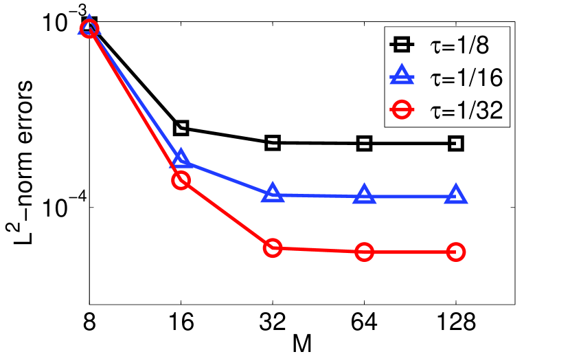
Figure 1: $L^{2}$-norm error with $r=2$

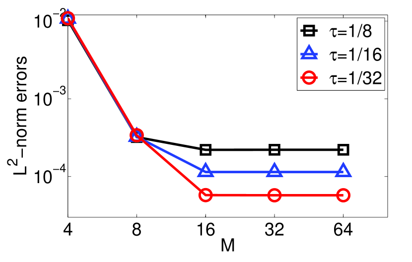
Figure 2: $L^{2}$-norm error with $r=3$.

6 Conclusion

In this paper, we have presented optimal error estimates for a linearized backward Euler–Galerkin FEM for a nonlinear and non-degenerate diffusion equation in a convex polygonal domain based on certain assumption on the regularity of the exact solution. For this strongly nonlinear equation, no previous works have been devoted to the error analysis for linearized semi-implicit FEMs, and existing analyses for implicit schemes still require certain restrictions on the time stepsize. Our analysis shows that the numerical solution of the linearized semi-implicit scheme achieves optimal convergence rate without any time-step condition.

There are some applications in which some degenerate diffusion equations ($\lambda=0$) should be investigated, such as total variation model [4, 20, 21] and parabolic $p$-Laplacian [3, 17, 36] without regularization. Numerical analysis for such degenerate equations is extremely difficult. Existing techniques in classical FEMs may not work well. Analysis for linearized schemes was less explored and many efforts focused only on implicit schemes and suboptimal error estimates due to the degeneracy. The extension of our analysis to the nonlinear non-degenerate diffusion equation in three-dimensional space and to the the nonlinear degenerate equations is our future works.

Appendix: $\bf H^{2+\delta_{0}}$ regularity of the equation $\bf\nabla\cdot(A(\nabla U^{n})\nabla\psi)=\varphi$

Under the assumption that $\|U^{n}\|_{H^{2+s_{0}}}\leq C$ (as given in Theorem 2.2) we consider the equation

$$\left\{\begin{array}[]{ll}\nabla\cdot(A(\nabla U^{n})\nabla\psi)=\varphi&\mbox{in}~{}~{}\Omega,\\[5.0pt] \nabla\psi\cdot{\vec{n}}=0&\mbox{on}~{}~{}\partial\Omega,\end{array}\right.$$ (A.3)

with the compatibility condition $\int_{\Omega}\varphi{\rm d}x=0$ and the normalization condition $\int_{\Omega}\psi{\rm d}x=0$.

For simplicity, we only present a priori estimates here. The equation can be written as

$$\Delta\psi=\frac{\nabla^{2}\psi\nabla U^{n}\cdot\nabla U^{n}}{\lambda^{2}+|\nabla U^{n}|^{2}}-\sqrt{1+|\nabla U^{n}|^{2}/\lambda^{2}}\partial_{i}A_{ij}(\nabla U^{n})\partial_{j}\psi+\sqrt{1+|\nabla U^{n}|^{2}/\lambda^{2}}\varphi$$ (A.4)

and by using (4.2) we derive that

$$\|\nabla^{2}\psi\|_{L^{2}} \leq\bigg{\|}\frac{|\nabla U^{n}|^{2}}{\lambda^{2}+|\nabla U^{n}|^{2}}\bigg{\|}_{L^{\infty}}\|\nabla^{2}\psi\|_{L^{2}}+C\|\nabla^{2}U^{n}\|_{L^{p}}\|\nabla\psi\|_{L^{\bar{p}}}+C\|\varphi\|_{L^{2}}$$

$$\leq\frac{K^{2}}{1+K^{2}}\|\nabla^{2}\psi\|_{L^{2}}+C\|\nabla\psi\|_{L^{\bar{p}}}+C\|\varphi\|_{L^{2}},$$

which further reduces to

$$\|\nabla^{2}\psi\|_{L^{2}} \leq C\|\nabla\psi\|_{L^{\bar{p}}}+C\|\varphi\|_{L^{2}}$$

$$\leq C\|\nabla\psi\|_{L^{2}}^{2/\bar{p}}\|\psi\|_{H^{2}}^{1-2/\bar{p}}+C\|\varphi\|_{L^{2}}$$

$$\leq\epsilon\|\psi\|_{H^{2}}+C_{\epsilon}\|\nabla\psi\|_{L^{2}}+C\|\varphi\|_{L^{2}}$$

$$\leq\epsilon\|\nabla^{2}\psi\|_{L^{2}}+C_{\epsilon}\|\varphi\|_{L^{2}}.$$

From the last inequality we see that

$$\|\psi\|_{H^{2}}\leq C\|\varphi\|_{L^{2}}.$$ (A.5)

Since $\nabla U^{n}\in H^{1+s_{0}}\hookrightarrow C^{s_{0}}(\overline{\Omega})$, it follows that

$$\begin{array}[]{ll}\displaystyle\Big{\|}\frac{F\nabla U^{n}\cdot\nabla U^{n}}{\lambda^{2}+|\nabla U^{n}|^{2}}\Big{\|}_{L^{2}}\leq\frac{K^{2}}{\lambda^{2}+K^{2}}\|F\|_{(L^{2})^{2\times 2}}&\mbox{for}~{}~{}s\in(0,s_{0}),\\[15.0pt] \displaystyle\Big{\|}\frac{F\nabla U^{n}\cdot\nabla U^{n}}{\lambda^{2}+|\nabla U^{n}|^{2}}\Big{\|}_{H^{s_{0}}}\leq C\|F\|_{(H^{s_{0}})^{2\times 2}}&\\[15.0pt] \|\sqrt{1+|\nabla U^{n}|^{2}/\lambda^{2}}\partial_{i}A_{ij}(\nabla U^{n})\partial_{j}\psi\|_{H^{s}}\leq C\|\psi\|_{H^{1+s}}&\mbox{for}~{}~{}s\in(0,s_{0}),\end{array}$$

and by the complex interpolation method [5] we derive that there exists a positive constant $\overline{s}_{0}\in(0,\min(s_{*},s_{0}))$ such that (where $s_{*}$ is given in (4.7))

$$\displaystyle\bigg{\|}\frac{F\nabla U^{n}\cdot\nabla U^{n}}{\lambda^{2}+|\nabla U^{n}|^{2}}\bigg{\|}_{H^{s}} \leq\bigg{(}\frac{K^{2}}{\lambda^{2}+K^{2}}\bigg{)}^{1-\bar{s}_{0}/s_{0}}C^{\bar{s}_{0}/s_{0}}\|F\|_{(H^{s})^{2\times 2}}$$

$$\leq\bigg{(}1-\frac{1}{2\lambda^{2}+2K^{2}}\bigg{)}\|F\|_{(H^{s})^{2\times 2}} \mbox{for}~{}~{}s\in(0,\overline{s}_{0}).$$

By applying (4.7) to (A.4) and using the last inequality, we derive that

$$\|\nabla^{2}\psi\|_{H^{s}}\leq(1+\overline{\varepsilon}_{s})\bigg{(}1-\frac{1}{2\lambda^{2}+2K^{2}}\bigg{)}\|\nabla^{2}\psi\|_{H^{s}}+C\|\psi\|_{H^{1+s}}+C\|\varphi\|_{H^{s}}\quad\mbox{for}~{}~{}s\in(0,\overline{s}_{0}).$$

There exists a positive constant $\delta_{0}$ such that $\overline{\varepsilon}_{s}<1/(2\lambda^{2}+2K^{2})$ when $s\in(0,\delta_{0}]$, and the last inequality reduces to

$$\|\nabla^{2}\psi\|_{H^{s}}\leq\bigg{(}1-\frac{1}{4(\lambda^{2}+K^{2})^{2}}\bigg{)}\|\nabla^{2}\psi\|_{H^{s}}+C\|\psi\|_{H^{1+s}}+C\|\varphi\|_{H^{s}}\quad\mbox{for}~{}~{}s\in(0,\delta_{0}].$$

which further implies that

$$\|\psi\|_{H^{2+s}}\leq C\|\varphi\|_{H^{s}}\quad\mbox{for}~{}~{}s\in(0,\delta_{0}].$$ (A.6)

References

[1]
E. Albrecht and V. Müller,
Spectrum of interpolated operators,
Proc.
Amer. Math. Soc.,
129 (2000), pp. 807–814.
[2]
A. Araujo, S. Barbeiro and P. Serranho,
Stability of finite difference schemes for complex diffusion processes,
SIAM J. Numer. Anal., 50 (2012), pp. 1284–1296.
[3]
J.W. Barrett and W.B. Liu,
Finite element approximation of the parabolic p-Laplacian,
SIAM J. Numer. Anal., 31(1994), 413–428.
[4]
G. Bellettini and V. Caselles, The total variation flow in , J. Differential Equations, 184 (2002), pp. 475–525.
[5]
J. Bergh and J. Löfström, Interpolation spaces: an introduction,
Springer-Verlag Berlin Heidelberg 1976, Printed in Germany.
[6]
C. Bernardi, M. Dauge and Y. Maday, Polynomials in the Sobolev
World, Preprint IRMAR 07-14, Rennes, March 2007.
[7]
D. Braess,
Finite Elements,
Theory, Fast Solvers, and Applications in Elasticity Theory,
Cambridge University Press, New York, 2007.
[8]
S.C. Brenner and L.R. Scott,
The Mathematical Theory of Finite Element Methods,
Third Edition, Springer Science+Business Media, LLC, 2008.
[9]
S.S. Byun and L. Wang, Elliptic equations with
measurable
coefficients in Reifenberg domains, Advances
in Mathematics,
225 (2010), pp. 2648–2673.
[10]
J. Calder, A. Mansouri and A. Yezzi,
Image sharpening via Sobolev gradient flows,
SIAM J. Imaging Sci., 3 (2010), pp. 981–1014.
[11]
A. Chambolle and P.L. Lions,
Image recovery via total variation minimization and related problems,
Numer. Math., 76 (1997), pp. 167–188.
[12]
T. Chan and J. Shen,
On the role of the BV image model in image
restoration, Tech. Report CAM 02-14, Department of Mathematics, UCLA, 2002.
[13]
C. Chen and G. Xu,
Gradient-flow-based semi-implicit finite-element method
and its convergence analysis for image reconstruction,
Inverse Problems, 28 (2012), pp. 035006–035024.
[14]
N. Chumchob and K. Chen,
Improved variational image registration model and a fast algorithm
for its numerical approximation,
Numer. Methods Partial Differential Eq.,
28 (2012), pp. 1966–1995.
[15]
M. Dauge,
Elliptic boundary value problems in corner domains,
Springer-Verlag Berlin Heidelberg, 1988.
[16]
K. Deckelnick and G. Dziuk,
Convergence of a finite element method for
non-parametric mean curvature,
Numer. Math., 72 (1995), pp. 197–222.
[17]
L. Diening, C. Ebmeyer and M. Ruzicka,
Optimal convergence for the implicit space-time
discretization of parabolic systems
with -structure,
SIAM J. Numer. Anal., 45 (2007), pp. 457–472.
[19]
C. Ebmeyer and J. Vogelgesang,
Finite element approximation of a forward and backward anisotropic
diffusion model in image denoising and form generalization,
Numer. Methods Partial Differential Eq., 24 (2008), pp. 646–662.
[20]
X. Feng and M. von Oehsen and A. Prohl,
Rate of convergence of regularization procedures and
finite element approximations for the total variation flow,
Numer. Math., 100 (2005), pp. 441–456.
[21]
X. Feng and A. Prohl,
Analysis of total variation flow and its finite element approximations,
M2AN Math. Model. Numer. Anal., 37 (2003), pp. 533–556.
[22]
X. Feng and A. Prohl, Analysis of gradient flow of a
regularized Mumford-Shah functional for image segmentation
and image inpainting, ESAIM: M2AN, 38 (2004), pp. 291–320.
[23]
C. Gerhardt,
Boundary value problems for surfaces of prescribed mean curvature,
J. Differential Equations, 36 (1980), pp. 139–172.
[24]
T. Grahs, A. Meister and T. Sonar,
Image processing for numerical approximations of
conservation laws: nonlinear anisotropic artificial dissipation,
SIAM J. Sci. Comput., 23 (2002), pp. 1439–1455.
[25]
P. Grisvard, Elliptic Problems in Nonsmooth Domains, SIAM 2011.
[26]
F. Hecht, New development in freefem++,
J. Numer. Math., 20 (2012), pp. 251–265.
[27]
B. Li and W. Sun,
Error analysis of linearized semi-implicit
Galerkin finite element methods for nonlinear parabolic equations,
Int. J. Numer. Anal.Modeling, 10 (2013), pp. 622–633.
[28]
B. Li and W. Sun, Unconditional convergence and optimal error
estimates of a Galerkin-mixed FEM for incompressible miscible flow
in porous media, SIAM J. Numer. Anal., 51 (2013), pp. 1949–1977.
[29]
A. Lichnewsky and R. Temam,
Pseudoslution of the time-dependent minimal surface problem,
J. Differential Equations, 30 (1978), pp. 340–364.
[30]
Z. Liu and Q. Chang,
Numerical analysis of the model of image processing
with time-delay regularization,
Appl. Math. Comput., 166 (2005), pp. 349–372.
[31]
Z. Liu and B. Guo,
New numerical algorithms for the nonlinear diffusion
model of image denoising
and segmentation,
Appl. Math. Comput., 178 (2006), pp. 380–389.
[32]
Z. Mghazli, Regularity of an elliptic problem with mixed
Dirichlet-Robin boundary conditions in a polygonal domain,
Calcolo, 29 (1992), pp. 241–267.
[33]
K. Mikula and F. Sgallari,
Semi-implicit finite volume scheme
for image processing in 3D cylindrical geometry,
J. Comp.
Appl.
Math., 161 (2003), pp. 119–132.
[34]
P. Perona and J. Malik,
Scale-space and edge detection using
anisotropic diffusion, IEEE transactions on pattern
analysis and
machine intelligence, 12 (1990), pp. 629–639.
[35]
R. Rannacher and R. Scott,
Some optimal error estimates for piecewise linear
finite element approximations,
Math. Comp., 38 (1982), pp. 437–445.
[36]
L.A. Vese and S.J. Osher,
Numerical methods for -harmonic flows and
applications to image processing,
SIAM J. Numer. Anal., 40 (2002), pp. 2085–2104.