Optimized Bit Mappings for Spatially Coupled LDPC Codes over Parallel Binary Erasure Channels

Abstract

In many practical communication systems, one binary encoder/decoder pair is used to communicate over a set of parallel channels. Examples of this setup include multi-carrier transmission, rate-compatible puncturing of turbo-like codes, and bit-interleaved coded modulation (BICM). A bit mapper is commonly employed to determine how the coded bits are allocated to the channels. In this paper, we study spatially coupled low-density parity check codes over parallel channels and optimize the bit mapper using BICM as the driving example. For simplicity, the parallel bit channels that arise in BICM are replaced by independent binary erasure channels (BECs). For two parallel BECs modeled according to a 4-PAM constellation labeled by the binary reflected Gray code, the optimization results show that the decoding threshold can be improved over a uniform random bit mapper, or, alternatively, the spatial chain length of the code can be reduced for a given gap to capacity. It is also shown that for rate-loss free, circular (tail-biting) ensembles, a decoding wave effect can be initiated using only an optimized bit mapper.

I Introduction

Spatial coupling of regular low-density parity check (LDPC) codes has emerged as a powerful technique to construct capacity-achieving codes for many communication channels using iterative belief propagation (BP) decoding [1, 2]. In this paper, we apply spatially coupled LDPC (SC-LDPC) codes to a system where communication takes place over a set of parallel channels. Parallel channels are frequently encountered in practical scenarios, including multi-carrier transmission and rate-compatible puncturing of turbo-like codes [3]. Our main motivation comes from the application of SC-LDPC codes to bit-interleaved coded modulation (BICM) systems, which are often analyzed under the assumption of equivalent parallel binary-input channels (or simply bit channels) [4, Sec. 2-C].

For a fixed code and channel characteristics, an important problem is how to allocate the coded bits to the channels. This allocation is performed by a so-called bit mapper. Our focus is on the asymptotic behavior and we are interested in optimizing the bit mapper in terms of the decoding threshold. The decoding threshold divides the parameter range used to characterize the quality of the set of parallel channels into a region where reliable decoding is possible and where it is not. Under the assumption of infinite codeword length, density evolution (DE) can be applied in order to find the threshold for LDPC codes and BP decoding [5].

SC-LDPC codes have been studied in the context of BICM systems in [6] and [7] assuming a uniform random bit mapping. Many authors have studied the optimization of bit mappers for irregular LDPC code ensembles. For example, in [8, 9], the authors use extrinsic information transfer charts to find approximate decoding thresholds and subsequently optimize bit mappers, where in [9] special attention is payed to the short block length regime. In [10], a downhill algorithm is used to find optimized bit mappings for two different LDPC codes. In [11], the authors substitute the parallel BICM bit channels by binary-input additive white Gaussian noise (AWGN) channels and optimized bit mappers are found for the codes and modulations specified in the DVB-T2 standard. Bit mappers with a simple implementation structure are designed in [12]. Some authors have also devised heuristic bit mapping strategies [13]. Furthermore, there exists a substantial amount of literature dealing with both code optimization for a fixed bit mapping (e.g., [14]) as well as the joint optimization of the code ensemble and the bit mapper (e.g., [15]).

In this paper, we take a similar approach as in [12] and substitute the parallel bit channels that arise in BICM with independent binary erasure channels (BECs). This is justified by the observation that the decoding threshold is mainly determined by the mutual information of the channel rather than the channel details, see the discussion in [12, Sec. I]. Compared to [11], where the parallel channels are approximated as binary-input AWGN channels, the numerical complexity of the DE equations is greatly simplified when studying BECs.

The results in this paper are for a scenario with two parallel BECs modeled according to a 4-PAM constellation labeled by the binary reflected Gray code (BRGC) and we also briefly discuss the generalization to an arbitrary number of channels. Optimized bit mappers are found for SC-LDPC code ensembles with a two-sided termination boundary [2, Sec. 2-B] as well as circular (tail-biting) ensembles [16, Sec. V]. For the two-sided ensembles, it is shown that the decoding threshold can be improved, or equivalently, the spatial chain length can be reduced for a given gap to capacity compared to a uniform random bit mapper. Circular ensembles on the other hand have a decoding behavior resembling that of regular uncoupled ensembles due to the absence of a termination boundary. We show that by using an optimized bit mapper, the different qualities of the parallel channels can be exploited to obtain a decoding wave effect as for two-sided ensembles, i.e., the channels are effectively used to induce a termination boundary.

II System Model

Figure 1: Block diagram of the considered system model.

We consider a communication system where one binary encoder/decoder pair is used to communicate over a set of parallel channels and a bit mapper determines the allocation of coded bits to the channels. A block diagram of the system model is shown in Fig. 1. In the following, the individual blocks are described in more detail.

II-A Parallel Channels

Many practical transmission scenarios can be modeled as a set of parallel channels and we take BICM as an example throughout this paper. To this end, consider the real AWGN channel $Y=X+N$, where $X\in\mathcal{X}$ is the channel input taking on values from a discrete signal constellation $\mathcal{X}$ and $N\sim\mathcal{N}(0,1)$. If we label each element in the constellation with a unique binary string of length $m=\log_{2}|\mathcal{X}|$, then, conceptually, we may view this setup as having $m$ parallel bit channels from $B_{i}$ to $Y$, where $B_{i}$, $1\leq i\leq m$, denotes the $i$th bit in the binary strings (counting from left to right) [4, Sec. 2-C]. Each of these bit channels can be characterized by an individual channel quality parameter $\alpha_{i}\triangleq 1-I(B_{i};Y)$ ranging from 0 (perfect channel) to 1 (useless channel). The mutual information $I(B_{i};Y)$ is commonly parameterized by the signal-to-noise ratio (SNR) and depends on the signal constellation as well as the binary labeling [4].

For simplicity, we replace these bit channels by parallel, independent BECs with erasure probabilities $\varepsilon_{i}=\alpha_{i}$. In Fig. 2, two PAM constellations labeled by the BRGC are shown, and in Fig. 3 we plot the corresponding $\varepsilon_{i}$ as a function of the average erasure probability $\mathrm{bar}{\varepsilon}=(\sum_{i=1}^{m}\varepsilon_{i})/m$. Note that $\mathrm{bar}{\varepsilon}$ (ranging from 0 to 1) is implicitly parameterized by the SNR (ranging from $+\infty$ dB to $-\infty$ dB), indicated by the top scale in Fig. 3, and this parameterization is different for the two constellations. Henceforth, $\mathrm{bar}{\varepsilon}$ is used as the parameter to characterize the overall quality of the set of parallel channels (cf. Fig. 1) and the correspondence between $\mathrm{bar}{\varepsilon}$ and the individual channel qualities is according to Fig. 3.

(a) 4-PAM

(b) 8-PAM

Figure 2: Two PAM constellations labeled by the BRGC.

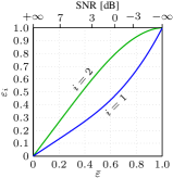
(a) 4-PAM, BRGC

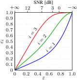
(b) 8-PAM, BRGC

Figure 3: Individual erasure probabilities $\varepsilon_{i}$ plotted over $\mathrm{bar}{\varepsilon}$.

II-B Encoder and Decoder

We focus on the two-sided and circular spatially coupled $(d_{\text{v}},d_{\text{c}},L,{w})$ code ensembles, where $d_{\text{v}}$ and $d_{\text{c}}$ denote the variable node (VN) and check node (CN) degrees, $L$ the spatial chain length, and ${w}$ is a “smoothing” parameter.

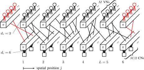
Figure 4: Graphical representation of the Tanner graph for the two-sided $(3,6,5,2)$ spatially coupled ensemble. Known VNs are shown in red.

The construction of the two-sided ensemble is explained in detail in [2, Sec. 2-B] and extended to circular ensembles in [16, Sec. V]. For completeness, we review the construction with the help of the example depicted in Fig. 4, where $d_{\text{v}}=3$, $d_{\text{c}}=6$, $L=5$, and ${w}=2$, starting with the two-sided case. $M$ VNs are placed at each spatial position $1$ to $L$ and $d_{\text{v}}M/d_{\text{c}}$ CNs are placed at each position $1$ to $L+{w}-1$. For the asymptotic case, i.e., infinite codeword length, it is assumed that $M\to\infty$. The red circles in Fig. 4 correspond to known VNs which are initialized to zero erasure probability and placed at positions $-w+2$ to $0$ and $L+1$ to $L+w-1$. The connections between VNs and CNs are as follows. It is assumed that the $d_{\text{v}}M$ edges originating from VNs at position $j$ are uniformly and independently distributed to CNs at positions $j$ to $j+{w}-1$, whereas the $d_{\text{v}}M$ edges from CNs at position $j$ are assumed to be uniformly and independently distributed to VNs at positions $j-{w}+1$ to $j$. In the figure, this is represented by the interleaver blocks that uniformly spread out the edges from the VNs and CNs. For circular ensembles, one can apply the same construction as above, but all position indices are now interpreted modulo $L$ and no known VNs are present [16, Sec. V]. For the example in Fig. 4, this would correspond to removing the red nodes and edges and appropriately connecting the VNs at position 5 to the CNs at position 1. Also, no CNs are placed at position 6 due to the modulo indexing.

The design rate $R$ of the two-sided ensemble is given by [2, Lemma 3]

$$R=1-\frac{d_{\text{v}}}{d_{\text{c}}}-\frac{d_{\text{v}}}{d_{\text{c}}}\frac{{w}+1-2\sum_{i=0}^{{w}}\left(\frac{i}{{w}}\right)^{d_{\text{c}}}}{L},$$ (1)

and it can be seen that there is a rate loss with respect to the design rate $1-d_{\text{v}}/d_{\text{c}}$ of the underlying regular ensemble. This is due to the termination boundary and the fact that a certain fraction of CNs is only connected to known VNs. For the circular ensemble, the rate loss is zero since all VNs and CNs are fully connected.

From the above definition of the ensemble, one can develop DE equations that describe the temporal and spatial evolution of the VN erasure probabilities when performing BP decoding under the assumption that $M\to\infty$. In this case, the VN erasure probabilities are given by [2, eq. (7)]

$$p^{(l+1)}_{j}=\varepsilon^{j}\left(\frac{1}{{w}}\sum_{a=0}^{{w}}\left(1-\left(1-\frac{1}{{w}}\sum_{b=0}^{{w}}p^{(l)}_{j+a-b}\right)^{d_{\text{c}}-1}\right)\right)^{d_{\text{v}}-1}$$ (2)

for $-{w}+2\leq j\leq L+{w}-1$, where $l$ denotes the iteration number and $\varepsilon^{j}$ the input erasure probability for the VNs at position $j$. The initial conditions for the two-sided ensemble are $p_{j}^{(0)}=\varepsilon^{j}$, where $\varepsilon^{j}=0$ for $j<1$ and $j>L$ due to the known VNs. For circular ensembles, $j\in\{1,\cdots,L\}$ and the index arithmetic in (2) is performed modulo $L$ [16, Sec. V].

II-C Bit Mapper and Demapper

For the considered scenario, the DE equations (2) are, in principle, the same as for the well-studied case with only one BEC. The only difference is that the input erasure probabilities can be different for each spatial position, i.e., one may think of the VNs at different positions belonging to different equivalence classes. One possible way to describe the assignment of channels to VN classes is via a matrix $\mathbf{A}=[a_{i,j}]\in\mathbb{R}^{m\times L}$, where $a_{i,j}$, $0\leq a_{i,j}\leq 1$ $\forall i,j$, denotes the fraction of VNs from position $j$ to be sent over the $i$th BEC. If we collect the individual channel erasure probabilities in a vector $\boldsymbol{\varepsilon}\triangleq(\varepsilon_{1},\dots,\varepsilon_{m})$, then, multiplying $\boldsymbol{\varepsilon}$ by $\mathbf{A}$ leads to a vector $(\varepsilon^{1},\varepsilon^{2},\dots,\varepsilon^{L})$ with the input erasure probabilities of the $L$ VN classes. Each input erasure probability is thus a weighted average of the channel erasure probabilities. In order to have a valid assignment, all columns in $\mathbf{A}$ have to sum up to one and all rows in $\mathbf{A}$ have to sum up to $L/m$. The first condition ensures that all VNs are assigned to a channel, while the second condition ensures that all parallel channels are used equally often. The set of valid assignment matrices that fulfill the above conditions is denoted by $\mathcal{A}^{m\times L}\subset\mathbb{R}^{m\times L}$.

III Decoding Threshold and Potential Gains

For a fixed bit mapper, i.e., for a fixed assignment matrix $\mathbf{A}$, the decoding threshold $\mathrm{bar}{\varepsilon}^{*}(\mathbf{A})$ is defined as the largest $\mathrm{bar}{\varepsilon}\in[0,1]$ such that $\lim_{l\to\infty}{p}^{(l)}_{j}={0}$, $1\leq j\leq L$, cf. (2). This condition corresponds to successful decoding, i.e., all erased VNs can be recovered using BP decoding. In practice, to obtain the threshold with a certain precision $\delta$, one fixes a target erasure probability $p_{\text{tar}}$ and a maximum number of iterations $l_{\text{max}}$. Then, starting from $\mathrm{bar}{\varepsilon}=\delta$, one iteratively computes (2) until the average erasure probability $(\sum_{j=1}^{L}p_{j}^{(l)})/L$ is either smaller than $p_{\text{tar}}$ (successful decoding) or the number of iterations exceeds $l_{\text{max}}$ (decoding failure). In the first case, $\mathrm{bar}{\varepsilon}$ is increased by $\delta$ until the decoding fails. For a given channel quality parameter $\mathrm{bar}{\varepsilon}$ up to the decoding threshold, we denote the number of iterations until successful decoding by $l_{\text{s}}(\mathbf{A},\mathrm{bar}{\varepsilon})$.

We are interested in optimizing $\mathbf{A}$ in terms of the decoding threshold for a given code ensemble. The baseline bit mapper realizes a uniform random mapping of coded bits to channels. For this case, we have $a_{i,j}=1/m$ $\forall i,j$, and the corresponding assignment matrix is denoted by $\mathbf{A}_{\text{uni}}$. To establish the amount of threshold gain we can hope for by finding a better $\mathbf{A}$, consider the following. Each BEC has capacity $C_{i}=1-\varepsilon_{i}$ and the average capacity is $\mathrm{bar}{C}=\frac{1}{m}\sum_{i=1}^{m}C_{i}=1-\mathrm{bar}{\varepsilon}$, where $1-\mathrm{bar}{\varepsilon}$ would correspond to the capacity of a BEC with erasure probability $\mathrm{bar}{\varepsilon}$. By employing the baseline mapper, however, the channel is effectively a BEC with erasure probability $\mathrm{bar}{\varepsilon}$ and the two-sided $(d_{\text{v}},d_{\text{c}},L,{w})$ ensemble can approach the capacity of this channel for appropriately chosen $(d_{\text{v}},d_{\text{c}})$ and $L\to\infty$, ${w}\to\infty$ [2, Th. 10]. Hence, for very long chain length $L$ and smoothing parameter ${w}$, one would expect the potential gains in terms of threshold improvement to be rather small. However, for finite $L$ and ${w}$, which is our main region of interest in this paper, significant gains may still be possible. This is also an important region for practical systems since increasing $L$ and ${w}$ leads to large block lengths (assuming a fixed and finite $M$) and high decoding complexity. Moreover, for the same average channel quality $\mathrm{bar}{\varepsilon}$, an optimized bit mapper may significantly reduce the number of decoding iterations until successful decoding compared to the baseline bit mapper. Finally, these potential gains come only at a small cost, i.e., by replacing the baseline bit mapper.

IV Optimization

Ideally, we would like to solve the problem

$$\mathbf{A}_{\text{opt}}=\underset{\mathbf{A}\in\mathcal{A}^{m\times L}}{\text{argmax}}\quad \mathrm{bar}{\varepsilon}^{*}(\mathbf{A}).$$ (3)

It was already pointed out in [17, Sec. IV] that directly optimizing a decoding threshold is difficult, simply due to the fact that finding the threshold is computationally expensive. This is especially pronounced for SC-LDPC codes and even for the moderate chain lengths considered in this paper ($L\leq 40$), the computational cost attached to one threshold computation is significant in the context of an optimization routine. An alternative, yet practical, approach, is to start with a certain channel quality parameter $\mathrm{bar}{\varepsilon}$ and then optimize the convergence behavior of the ensemble in terms of decoding iterations. Then, one can calculate the new threshold for the obtained assignment matrix and repeat the whole procedure. Such an iterative approach was proposed in [17, Sec. IV] to find optimized degree distributions for irregular LDPC codes. Based on this idea, we use the following iterative optimization routine in order to find bit mappers with good decoding thresholds.

1. Initialize the channel quality $\mathrm{bar}{\varepsilon}$ to the decoding threshold for the baseline bit mapper, i.e., $\mathrm{bar}{\varepsilon}=\mathrm{bar}{\varepsilon}^{*}(\mathbf{A}_{\text{uni}})$.

2. Find $\mathbf{A\!{}^{*}}$ such that it minimizes the number of decoding iterations until convergence for the given channel quality $\mathrm{bar}{\varepsilon}$, i.e.,

   $$\mathbf{A\!{}^{*}}=\underset{\mathbf{A}\in\mathcal{A}^{m\times L}}{\text{argmin}}\quad l_{\text{s}}(\mathbf{A},\mathrm{bar}{\varepsilon}).$$ (4)

   To solve the optimization problem (4), we use differential evolution [18].

3. For the found optimized $\mathbf{A\!{}^{*}}$, calculate the new threshold $\mathrm{bar}{\varepsilon}^{*}(\mathbf{A\!{}^{*}})$. If the threshold did not improve, stop. Otherwise, set $\mathrm{bar}{\varepsilon}=\mathrm{bar}{\varepsilon}^{*}(\mathbf{A\!{}^{*}})$ and go to step 2).

With this procedure, the computational complexity can be significantly reduced. However, it is not guaranteed to be equivalent to a true threshold optimization, i.e., $\mathbf{A}_{\text{opt}}\neq\mathbf{A\!{}^{*}}$ in general.

V Results and Discussion

In the following, we present optimization results assuming two parallel BECs according to Fig. 3(a). We focus on the two-sided and circular versions of the $(4,8,L,{w})$ ensemble, where $L\in\{10,15,\ldots,40\}$ and ${w}\in\{2,4\}$. Threshold values are computed assuming $\delta=10^{-4}$, $p_{\text{tar}}=10^{-6}$, and $l_{\text{max}}=5000$. For a code ensemble with design rate $R$ and an assignment matrix $\mathbf{A}$, the gap to capacity is defined as $\Delta\triangleq 1-\mathrm{bar}{\varepsilon}^{*}(\mathbf{A})-R$.

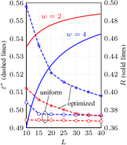
(a) Threshold and Design Rate

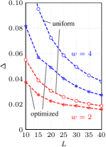
(b) Gap to Capacity

Figure 5: Optimization results for the two-sided $(4,8,L,{w})$ ensemble. Color is helpful.

V-A Two-Sided Ensembles

In Fig. 5, the results for the two-sided ensembles are shown. Fig. 5(a) shows both the decoding threshold (solid lines) and the design rate (dashed lines) and Fig. 5(b) shows the corresponding gap to capacity. The red and blue lines correspond to ${w}=2$ and ${w}=4$, respectively.

Let us first briefly discuss the performance behavior for the uniform baseline bit mapping schemes (circle markers), which is essentially the same as for the case with only one BEC. Both ensembles converge rapidly to a fixed threshold value for increased chain lengths, i.e., for $L\geq 15$ the decoding threshold is approximately $0.497$ and $0.494$ for ${w}=2$ and ${w}=4$, respectively. Furthermore, the ensemble with stronger coupling $({w}=4)$ exhibits a significantly larger rate loss.

The thresholds that can be achieved with the optimized bit mappers are shown by the star markers. It can be observed that it is possible to improve over the “uniform” thresholds and, as expected, the absolute threshold improvement becomes smaller with increasing chain length. For $L\to\infty$, it was already mentioned that the expected threshold gains will tend to zero. The results shown in Fig. 5(b) incorporate both the design rate and the decoding threshold and allow for a comparison between the two coupling parameters. We can conclude that a small coupling parameter is beneficial in terms of $\Delta$, due to the large rate loss for ${w}=4$ for both the uniform and optimized bit mappers. Moreover, for a fixed gap to capacity, the optimized bit mappers allow for a significant chain length reduction. As an example, for $\Delta=0.04$ and ${w}=4$, the chain length can be reduced from approximately $L=40$ to $L=25$ and for $\Delta=0.02$ and ${w}=2$ a chain length reduction from $L=35$ to $L=25$ is possible.

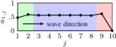
(a) $L=10$

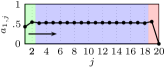
(b) $L=20$

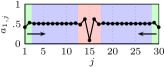
(c) $L=30$

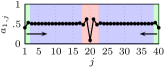
(d) $L=40$

Figure 6: Values in the first row of the optimized assignment matrices $\mathbf{A\!{}^{*}}$ for the two-sided $(4,8,L,2)$ ensemble with different chain lengths.

Next, we show some of the found optimized bit mappers and discuss their structure and the resulting iterative decoding behavior. In Fig. 6, the values in the first row of the optimized assignment matrices $\mathbf{A\!{}^{*}}$ are plotted for ${w}=2$ and spatial lengths $L\in\{10,20,30,40\}$. The values in the first row (i.e., $i=1$) determine the fraction of VNs at a particular position to be sent over the good channel, cf. Fig. 3(a). Certain regions of the spatial dimension are shaded in different colors and, when $\mathrm{bar}{\varepsilon}=\mathrm{bar}{\varepsilon}^{*}(\mathbf{A\!{}^{*}})$, these regions correspond to the part where a so-called decoding wave will start (green), end (red), and propagate at a roughly constant speed (blue). First, let us focus on Fig. 6(a) to gain some insight into the general structure of the optimized bit mappers. It is visible that the VNs at the last position are allocated only to the bad channel and there are proportionally more VNs allocated to the bad channel at the first position (i.e., $a_{1,1}$ is slightly less than $0.5$). For the positions shaded in blue, the values of the assignment matrix are roughly constant. Similar observations can be made for $L=20$. To illustrate the effect of the optimized bit mappers, in Fig. 7(a) we provide a visualization of the iterative decoding behavior for the two-sided $(4,8,20,2)$ ensemble at the threshold value of $\mathrm{bar}{\varepsilon}^{*}(\mathbf{A\!{}^{*}})=0.5024$. As seen from the figure, the optimized bit mapper induces a one-sided wave propagation even though the ensemble is two-sided, and the wave propagates at a roughly constant speed. The direction of the wave is arbitrary due to the symmetry of the Tanner graph describing the ensemble, i.e., flipping each row in the assignment matrix leads to a wave propagating from right to left with otherwise unchanged behavior.

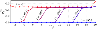
(a) two-sided, $\mathrm{bar}{\varepsilon}^{*}(\mathbf{A\!{}^{*}})=0.5024$, $R=0.4752$, $\Delta=0.0224$

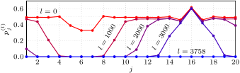
(b) circular, $\mathrm{bar}{\varepsilon}^{*}(\mathbf{A\!{}^{*}})=0.4772$, $R=0.5$, $\Delta=0.0228$

Figure 7: Visualization of the iterative decoding behavior for (a) the two-sided and (b) the circular version of the $(4,8,20,2)$ ensemble with optimized bit mappers. The optimized bit mapper induces a one-sided wave propagation for the two-sided ensemble in (a).

The general structure of the optimized bit mappers for $L\in\{15,25\}$ is similar to the ones shown in Fig. 6(a) and (b). For $L>25$, the structure changes as indicated in Fig. 6(c) and (d) for $L=30$ and $L=40$, respectively. Here, the optimized allocation is such that two decoding waves propagate from the ends of the spatial chain towards the center, similarly as for a uniform bit mapper. The different structure occurring for larger values of $L$ is possibly due to the fact that a two-sided wave propagation leads to a faster convergence compared to one-sided propagation for a given chain length $L$, even though a one-sided propagation may be better in terms of threshold. However, due to the fixed maximum number of decoding iterations, the iterative optimization routine converges to these solutions for larger $L$.

From the structure of the optimized bit mappers, an intuitive explanation for the decoding threshold improvement can be given as follows. In some sense, certain VN classes are “overprotected” and proportionally more of the VNs from these classes can be allocated to the bad channel without harming the overall iterative decoding performance. In turn, this allows for the remaining VN classes to be allocated more to the good channel, i.e., channel uses corresponding to the good channel become available and are spread out evenly among the VNs in the regions indicated in blue. In fact, all optimized bit mappers for ${w}=2$ are such that in the blue regions, the values for $a_{1,j}$ are all slightly greater than $0.5$. From this one can also explain why asymptotically the threshold gain will tend to zero, since asymptotically as $L\to\infty$ this effect is not noticeable any more and $a_{1,j}\to 0.5$ in the blue regions.

The optimized bit mappers for ${w}=4$ in principle show a similar structure, but tend to be more unstable and wiggle around a certain average value in the part of the spatial chain that is shaded in blue.

V-B Circular Ensembles

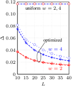
(a) Gap to Capacity

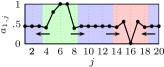
(b) $L=20$

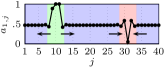
(c) $L=40$

Figure 8: Optimization results for the circular $(4,8,L,{w})$ ensemble. In (b) and (c), we plot the values in the first row of the optimized assignment matrices for ${w}=2$. Color is helpful.

In Fig. 8, we show the optimization results for the circular ensembles. In Fig. 8(a), the performance of the uniform and optimized bit mappers is shown in terms of the gap to capacity. The dotted lines correspond to the performance of the optimized bit mappers for the two-sided case and are simply reproduced from Fig. 5(b) for convenience to allow for a comparison between the two-sided and circular ensembles. For circular ensembles, the design rate is $R=1/2$, independent of $L$, and the decoding threshold assuming a uniform bit mapper is given by $\mathrm{bar}{\varepsilon}^{*}(\mathbf{A}_{\text{uni}})=0.3834$ for both coupling parameters, hence the constant “uniform” gap to capacity in Fig. 8(a). In fact, this threshold value corresponds to the BP decoding threshold of the regular, uncoupled $(4,8)$ ensemble due to the absence of a termination boundary. By employing the optimized bit mappers, a significant threshold gain is possible, which directly translates into a significant reduction in terms of the gap to capacity. Contrary to the two-sided case, the threshold gain with respect to a uniform bit mapper increases for longer chain lengths $L$. Compared to the results for the two-sided ensembles, one can achieve a slightly better performance for ${w}=4$, while for ${w}=2$, the corresponding curves in Fig. 8(a) virtually overlap. The improvement for ${w}=4$ can be explained by the large rate loss for the two-sided ensemble, and it shows that a more careful design of the termination boundary for small $L$ may be beneficial to achieve a better trade-off between rate loss and decoding threshold performance.

Similarly as before, in Fig. 8(b) and (c), we show some of the optimized bit mappers in the form of the values in the first row of $\mathbf{A\!{}^{*}}$ for ${w}=2$ and $L\in\{20,40\}$. The actual results from the optimization routine have been adjusted (i.e., appropriately flipped and shifted), so as to make the figures look similar. It can be observed that for circular ensembles, the optimized bit mappers are such that the VNs over a small spatial range in the green region are exclusively allocated to the good channel. In the red regions, the optimized allocation resembles that of the two-sided ensembles for $L\in\{30,40\}$, cf. Fig. 6(c) and (d). The resulting iterative decoding behavior is illustrated in Fig. 7(b) for the circular version of the $(4,8,20,2)$ ensemble at the decoding threshold value of $\mathrm{bar}{\varepsilon}^{*}(\mathbf{A\!{}^{*}})=0.4772$. In essence, the different channel qualities are exploited and a virtual termination boundary is created by the optimized bit mapping schemes. This allows for local convergence of the BP decoder at these positions within the first few iterations and consequently two waves propagate outwards and eventually end in the region shaded in red.

V-C Extension to More than Two Channels

An extension to scenarios where more than two channels are present, e.g., for three BECs as shown in Fig. 3(b), is straightforward but comes at the price of increased optimization complexity due to the dimensionality increase of the problem. However, once a good bit mapper for two BECs is found, one can easily try the following. Let $\mathbf{A\!{}^{*}}\in\mathcal{A}^{2\times L}$ be an optimized assignment matrix for a given code ensemble of length $L$ and $\mathrm{bar}{\varepsilon}^{*}(\mathbf{A\!{}^{*}})$ the corresponding threshold. The input erasure probabilities for the VNs $(\varepsilon^{1},\dots,\varepsilon^{L})$ are thus fixed. One can then try to find a feasible $\mathbf{A}\in\mathcal{A}^{3\times L}$ that satisfies $\boldsymbol{\varepsilon}\mathbf{A}=(\varepsilon^{1},\dots,\varepsilon^{L})$, where $\boldsymbol{\varepsilon}=(\varepsilon_{1},\varepsilon_{2},\varepsilon_{3})$ is a vector with the individual erasure probabilities for $\mathrm{bar}{\varepsilon}=\mathrm{bar}{\varepsilon}^{*}(\mathbf{A\!{}^{*}})$ in Fig. 3(b). This can be accomplished using standard numerical optimization routines.

VI Conclusion and Future Work

In this paper, we studied SC-LDPC code ensembles over parallel channels. Motivated by BICM, we used an example with two parallel BECs and optimized the bit mapper that determines the allocation of coded bits to the channels. Compared to a uniform random bit mapper, the decoding threshold can be improved or, alternatively, the spatial chain length can be reduced. For circular ensembles, the different qualities of the channels can be exploited to obtain a wave-like decoding behavior similar to terminated, e.g., two-sided, ensembles. Future work includes the study of protograph-based ensembles for finite length code design and the application to different channel types. Further, it would be of much practical value to find an analytical characterization of the optimal mappers.

References

- [1] M. Lentmaier, A. Sridharan, K. S. Zigangirov, and D. J. Costello, “Terminated LDPC convolutional codes with thresholds close to capacity,” in Proc. IEEE Int. Symp. Information Theory (ISIT), Adelaide, Australia, Sep. 2005.
- [2] S. Kudekar, T. Richardson, and R. Urbanke, “Threshold saturation via spatial coupling: Why convolutional LDPC ensembles perform so well over the BEC,” IEEE Trans. Inf. Theory, vol. 57, no. 2, pp. 803–834, Feb. 2011.
- [3] I. Sason and I. Goldenberg, “Coding for parallel channels: Gallager bounds and applications to turbo-like codes,” IEEE Trans. Inf. Theory, vol. 53, no. 7, pp. 2394–2428, Jul. 2007.
- [4] G. Caire, G. Taricco, and E. Biglieri, “Bit-interleaved coded modulation,” IEEE Trans. Inf. Theory, vol. 44, no. 3, pp. 927–946, May 1998.
- [5] T. Richardson and R. Urbanke, “The capacity of low-density parity-check codes under message-passing decoding,” IEEE Trans. Inf. Theory, vol. 47, no. 2, pp. 599–618, Feb. 2001.
- [6] L. Schmalen and S. ten Brink, “Combining spatially coupled LDPC codes with modulation and detection,” in Proc. Int. Conf. Systems, Communication and Coding (SCC), Munich, Germany, Jan. 2013.
- [7] A. Yedla, M. El-Khamy, J. Lee, and I. Kang, “Performance of spatially-coupled LDPC codes and threshold saturation over BICM channels,” arXiv:1303.0296v1 [cs.IT], Mar. 2013. [Online]. Available: http://arxiv.org/abs/1303.0296
- [8] T. Cheng, K. Peng, J. Song, and K. Yan, “EXIT-aided bit mapping design for LDPC coded modulation with APSK constellations,” IEEE Commun. Lett., vol. 16, no. 6, pp. 777–780, Jun. 2012.
- [9] S. Nowak and R. Kays, “On matching short LDPC codes with spectrally-efficient modulation,” in Proc. IEEE Int. Symp. Information Theory (ISIT), Cambridge, MA, Jul. 2012.
- [10] G. Richter, A. Hof, and M. Bossert, “On the mapping of low-density parity-check codes for bit-interleaved coded modulation,” in Proc. IEEE Int. Symp. Information Theory (ISIT), Nice, Italy, Jun. 2007.
- [11] L. Gong, S. Member, L. Gui, B. Liu, and B. Rong, “Improve the performance of LDPC coded QAM by selective bit mapping in terrestrial broadcasting system,” IEEE Trans. Broadcast., vol. 57, no. 2, pp. 263–269, Jun. 2011.
- [12] J. Lei, W. Gao, P. Spasojevic, and R. Yates, “Demultiplexer design for multi-edge type LDPC coded modulation,” in Proc. IEEE Int. Symp. Information Theory (ISIT), Seoul, South Korea, Jun. 2009.
- [13] W. Li Yan, Ryan, “Bit-reliability mapping in LDPC-coded modulation systems,” IEEE Commun. Lett., vol. 9, no. 1, pp. 1–3, Jan. 2005.
- [14] J. Hou, P. H. Siegel, L. B. Milstein, and H. D. Pfister, “Capacity-approaching bandwidth-efficient coded modulation schemes based on low-density parity-check codes,” IEEE Trans. Inf. Theory, vol. 49, no. 9, pp. 2141–2155, Sep. 2003.
- [15] G. Durisi, L. Dinoi, and S. Benedetto, “eIRA codes for coded modulation systems,” in Proc. IEEE Int. Conf. Communications (ICC), Istanbul, Turkey, Jun. 2006.
- [16] S. Kudekar, C. Méasson, T. J. Richardson, and R. L. Urbanke, “Threshold saturation on BMS channels via spatial coupling,” in Proc. Int. Symp. Turbo Codes and Iterative Information Processing (ISTC), Le Quartz, France, Sep. 2010.
- [17] T. J. Richardson, M. A. Shokrollahi, and R. L. Urbanke, “Design of capacity-approaching irregular low-density parity-check codes,” IEEE Trans. Inf. Theory, vol. 47, no. 2, pp. 619–637, Feb. 2001.
- [18] R. Storn and K. Price, “Differential evolution–a simple and efficient heuristic for global optimization over continuous spaces,” J. Global Opt., pp. 341–359, Nov. 1997.