Structured learning of sum-of-submodular higher order energy functions

Abstract

Submodular functions can be exactly minimized in polynomial time, and the special case that graph cuts solve with max flow [18] has had significant impact in computer vision [5, 20, 27]. In this paper we address the important class of sum-of-submodular (SoS) functions [2, 17], which can be efficiently minimized via a variant of max flow called submodular flow [6]. SoS functions can naturally express higher order priors involving, e.g., local image patches; however, it is difficult to fully exploit their expressive power because they have so many parameters. Rather than trying to formulate existing higher order priors as an SoS function, we take a discriminative learning approach, effectively searching the space of SoS functions for a higher order prior that performs well on our training set. We adopt a structural SVM approach [14, 33] and formulate the training problem in terms of quadratic programming; as a result we can efficiently search the space of SoS priors via an extended cutting-plane algorithm. We also show how the state-of-the-art max flow method for vision problems [10] can be modified to efficiently solve the submodular flow problem. Experimental comparisons are made against the OpenCV implementation of the GrabCut interactive segmentation technique [27], which uses hand-tuned parameters instead of machine learning. On a standard dataset [11] our method learns higher order priors with hundreds of parameter values, and produces significantly better segmentations. While our focus is on binary labeling problems, we show that our techniques can be naturally generalized to handle more than two labels.

1 Introduction

Discrete optimization methods such as graph cuts [5, 18] have proven to be quite effective for many computer vision problems, including stereo [5], interactive segmentation [27] and texture synthesis [20]. The underlying optimization problem behind graph cuts is a special case of submodular function optimization that can be solved exactly using max flow [18]. Graph cut methods, however, are limited by their reliance on first-order priors involving pairs of pixels, and there is considerable interest in expressing priors that rely on local image patches such as the popular Field of Experts model [26].

In this paper we focus on an important generalization of the functions that graph cuts can minimize, which can express higher-order priors. These functions, which [17] called Sum-of-Submodular (SoS), can be efficiently solved with a variant of max flow [6]. While SoS functions have more expressive power, they also involve a large number of parameters. Rather than addressing the question of which existing higher order priors can be expressed as an SoS function, we take a discriminative learning approach and effectively search the space of SoS functions with the goal of finding a higher order prior that gives strong results on our training set.

Our main contribution is to introduce the first learning method for training such SoS functions, and to demonstrate the effectiveness of this approach for interactive segmentation using learned higher order priors. Following a Structural SVM approach [14, 33], we show that the training problem can be cast as a quadratic optimization problem over an extended set of linear constraints. This generalizes large-margin training of pairwise submodular (a.k.a. regular [18]) MRFs [1, 29, 30], where submodularity corresponds to a simple non-negativity constraint. To solve the training problem, we show that an extended cutting-plane algorithm can efficiently search the space of SoS functions.

1.1 Sum-of-Submodular functions and priors

A submodular function $f:2^{V}\to\mathbb{R}$ on a set $V$ satisfies $f(S\cap T)+f(S\cup T)\leq f(S)+f(T)$ for all $S,T\subseteq V$. Such a function is sum-of-submodular (SoS) if we can write it as

$$f(S)=\sum_{C\in\mathcal{C}}f_{C}(S\cap C)$$ (1)

for $\mathcal{C}\subseteq 2^{V}$ where each $f_{C}:2^{C}\to\mathbb{R}$ is submodular. Research on higher-order priors calls $C\in\mathcal{C}$ a clique [13].

Of course, a sum of submodular functions is itself submodular, so we could use general submodular optimization to minimize an SoS function. However, general submodular optimization is $O(n^{6})$ [25] (which is impractical for low-level vision problems), whereas we may be able to exploit the neighborhood structure $\mathcal{C}$ to do better. For example, if all the cliques are pairs ($|C|=2$) the energy function is referred to as regular and the problem can be reduced to max flow [18]. As mentioned above, this is the underlying technique used in the popular graph cuts approach [5, 20, 27]. The key limitation is the restriction to pairwise cliques, which does not allow us to naturally express important higher order priors such as those involving image patches [26]. The most common approach to solving higher-order priors with graph cuts, which involves transformation to pairwise cliques, in practice almost always produces non-submodular functions that cannot be solved exactly [8, 13].

2 Related Work

Many learning problems in computer vision can be cast as structured output prediction, which allows learning outputs with spatial coherence. Among the most popular generic methods for structured output learning are Conditional Random Fields (CRFs) trained by maximum conditional likelihood [22], Maximum-Margin Markov Networks (M3N) [32], and Structural Support Vector Machines (SVM-struct) [33, 14]. A key advantage of M3N and SVM-struct over CRFs is that training does not require computation of the partition function. Among the two large-margin approaches M3N and SVM-struct, we follow the SVM-struct methodology since it allows the use of efficient inference procedures during training.

In this paper, we will learn submodular discriminant functions. Prior work on learning submodular functions falls into three categories: submodular function regression [3], maximization of submodular discriminant functions, and minimization of submodular discriminant functions.

Learning of submodular discriminant functions where a prediction is computed through maximization has widespread use in information retrieval, where submodularity models diversity in the ranking of a search engine [34, 23] or in an automatically generated abstract [28]. While exact (monotone) submodular maximization is intractible, approximate inference using a simple greedy algorithm has approximation guarantees and generally excellent performance in practice.

The models considered in this paper use submodular discriminant functions where a prediction is computed through minimization. The most popular such models are regular MRFs [18]. Traditionally, the parameters of these models have been tuned by hand, but several learning methods exist. Most closely related to the work in this paper are Associative Markov Networks [30, 1], which take an M3N approach and exploit the fact that regular MRFs have an integral linear relaxation. These linear programs (LP) are folded into the M3N quadratic program (QP) that is then solved as a monolithic QP. In contrast, SVM-struct training using cutting planes for regular MRFs [29] allows graph cut inference also during training, and [7, 19] show that this approach has interesting approximation properties even the for multi-class case where graph cut inference is only approximate. More complex models for learning spatially coherent priors include separate training for unary and pairwise potentials [21], learning MRFs with functional gradient boosting [24], and the ${\cal P}^{n}$ Potts models, all of which have had success on a variety of vision problems. Note that our general approach for learning multi-label SoS functions, described in section 4.4, includes the ${\cal P}^{n}$ Potts model as a special case.

3 SoS minimization

In this section, we briefly summarize how an SoS function can be minimized by means of a submodular flow network (section 3.1), and then present our improved algorithm for solving this minimization (section 3.2).

3.1 SoS minimization via submodular flow

Submodular flow is similar to the max flow problem, in that there is a network of nodes and arcs on which we want to push flow from $s$ to $t$. However, the notion of residual capacity will be slightly modified from that of standard max flow. For a much more complete description see [17].

We begin with a network $G=(V\cup\{s,t\},A)$. As in the max flow reduction for Graph Cuts, there are source and sink arcs $(s,i)$ and $(i,t)$ for every $i\in V$. Additionally, for each clique $C$, there is an arc $(i,j)_{C}$ for each $i,j\in C$.

Every arc $a\in A$ also has an associated residual capacity $\overline{c}_{a}$. The residual capacity of arcs $(s,i)$ and $(i,t)$ are the familiar residual capacities from max flow: there are capacities $c_{s,i}$ and $c_{i,t}$ (determined by the unary terms of $f$), and whenever we push flow on a source or sink arc, we decrease the residual capacity by the same amount.

For the interior arcs, we need one further piece of information. In addition to residual capacities, we also keep track of residual clique functions $\overline{f}_{C}(S)$, related to the flow values by the following rule: whenever we push $\delta$ units of flow on arc $(i,j)_{C}$, we update $\overline{f}_{C}(S)$ by

$$\overline{f}_{C}(S)\leftarrow\left\{\begin{array}[]{ll}\overline{f}_{C}(S)-\delta&i\in S,j\notin S\\ \overline{f}_{C}(S)+\delta&i\notin S,j\in S\\ \overline{f}_{C}(S)&\mathrm{otherwise}\end{array}\right.$$ (2)

The residual capacities of the interior arcs are chosen so that the $\overline{f}_{C}$ are always nonnegative. Accordingly, we define $\overline{c}_{i,j,C}=\min_{S}\{\overline{f}_{C}(S)\mid i\in S,j\notin S\}$.

Given a flow $\phi$, define the set of residual arcs $A_{\phi}$ as all arcs $a$ with $\overline{c}_{a}>0$. An augmenting path is an $s-t$ path along arcs in $A_{\phi}$. The following theorem of [17] tells how to optimize $f$ by computing a flow in $G$.

Theorem 3.1.

Let $\phi$ be a feasible flow such that there is no augmenting path from $s$ to $t$. Let $S^{\ast}$ be the set of all $i\in V$ reachable from $s$ along arcs in $A_{\phi}$. Then $f(S^{\ast})$ is the minimum value of $f$ over all $S\subseteq V$.

3.2 IBFS for Submodular Flow

Incremental Breadth First Search (IBFS) [10], which is the state of the art in max flow methods for vision applications, improves the algorithm of [4] to guarantee polynomial time complexity. We now show how to modify IBFS to compute a maximum submodular flow in $G$.

IBFS is an augmenting paths algorithm: at each step, it finds a path from $s$ to $t$ with positive residual capacity, and pushes flow along it. Additionally, each augmenting path found is a shortest $s$-$t$ path in $A_{\phi}$. To ensure that the paths found are shortest paths, we keep track of distances $d_{s}(i)$ and $d_{t}(i)$ from $s$ to $i$ and from $i$ to $t$, and search trees $S$ and $T$ containing all nodes at distance at most $D_{s}$ from $s$ or $D_{t}$ from $t$ respectively. Two invariants are maintained:

• For every $i$ in $S$, the unique path from $s$ to $i$ in $S$ is a shortest $s$-$i$ path in $A_{\phi}$.

• For every $i$ in $T$, the unique path from $i$ to $t$ in $T$ is a shortest $i$-$t$ path in $A_{\phi}$.

The algorithm proceeds by alternating between forward passes and reverse passes. In a forward pass, we attempt to grow the source tree $S$ by one layer (a reverse pass attempts to grow $T$, and is symmetric). To grow $S$, we scan through the vertices at distance $D_{s}$ away from $s$, and examine each out-arc $(i,j)$ with positive residual capacity. If $j$ is not in $S$ or $T$, then we add $j$ to $S$ at distance level $D_{s}+1$, and with parent $i$. If $j$ is in $T$, then we found an augmenting path from $s$ to $t$ via the arc $(i,j)$, so we can push flow on it.

The operation of pushing flow may saturate some arcs (and cause previously saturated arcs to become unsaturated). If the parent arc of $i$ in the tree $S$ or $T$ becomes saturated, then $i$ becomes an orphan. After each augmentation, we perform an adoption step, where each orphan finds a new parent. The details of the adoption step are similar to the relabel operation of the Push-Relabel algorithm, in that we search all potential parent arcs in $A_{\phi}$ for the neighbor with the lowest distance label, and make that node our new parent.

In order to apply IBFS to the submodular flow problem, all the basic datastructures still make sense: we have a graph where the arcs $a$ have residual capacities $\overline{c}_{a}$, and a maximum flow has been found if and only if there is no longer any augmenting path from $s$ to $t$.

The main change for the submodular flow problem is that when we increase flow on an edge $(i,j)_{C}$, instead of just affecting the residual capacity of that arc and the reverse arc, we may also change the residual capacities of other arcs $(i^{\prime},j^{\prime})_{C}$ for $i^{\prime},j^{\prime}\in C$. However, the following result ensures that this is not a problem.

Lemma 3.2.

If $(a,b)_{C}$ was previously saturated, but now has residual capacity as a result of increasing flow along $(c,d)$, then (1) either $a=d$ or there was an arc $(a,d)\in A_{\phi}$ and (2) either $b=c$ or there was an arc $(c,b)\in A_{\phi}$.

Corollary 3.3.

Increasing flow on an edge never creates a shortcut between $s$ and $i$, or from $i$ to $t$.

The proofs are based on results of [9], and can be found in the Supplementary Material.

Corollary 3.3 ensures that we never create any new shorter $s$-$i$ or $i$-$t$ paths not contained in $S$ or $T$. A push operation may cause some edges to become saturated, but this is the same problem as in the normal max flow case, and any orpans so created will be fixed in the adoption step. Therefore, all invariants of the IBFS algorithm are maintained, even in the submodular flow case.

One final property of the IBFS algorithm involves the use of the “current arc heuristic”, which is a mechanism for avoiding iterating through all possible potential parents when performing an adoption step. In the case of Submodular Flows, it is also the case that whenever we create new residual arcs we maintain all invariants related to this current arc heuristic, so the same speedup applies here. However, as this does not affect the correctness of the algorithm, and only the runtime, we will defer the proof to the Supplementary Material.

Running time. The asymptotic complexity of the standard IBFS algorithm is $O(n^{2}m)$. In the submodular-flow case, we still perform the same number of basic operations. However, note finding residual capacity of an arc $(i,j)_{C}$ requires minimizing $\overline{f}_{C}(S)$ for $S$ separating $i$ and $j$. If $|C|=k$, this can be done in time $O(k^{6})$ using [25]. However, for $k<<n$, it will likely be much more efficient to use the $O(2^{k})$ naive algorithm of searching through all values of $\overline{f}_{C}$. Overall, we add $O(2^{k})$ work at each basic step of IBFS, so if we have $m$ cliques the total runtime is $O(n^{2}m2^{k})$.

This runtime is better than the augmenting paths algorithm of [2] which takes time $O(nm^{2}2^{k})$. Additionally, IBFS has been shown to be very fast on typical vision inputs, independent of its asymptotic complexity [10].

4 S3SVM: SoS Structured SVMs

In this section, we first review the SVM algorithm and its associated Quadratic Program (section 4.1). We then decribe a general class of SoS discriminant functions which can be learned by SVM-struct (section 4.2) and explain this learning procedure (section 4.3). Finally, we generalize SoS functions to the multi-label case (section 4.4).

4.1 Structured SVMs

Structured output prediction describes the problem of learning a function $h:{\cal X}\longrightarrow{\cal Y}$ where ${\cal X}$ is the space of inputs, and ${\cal Y}$ is the space of (multivariate and structured) outputs for a given problem. To learn $h$, we assume that a training sample of input-output pairs ${S}=((x_{1},y_{1}),\dots,(x_{n},y_{n}))\in({\cal X}\times{\cal Y})^{n}$ is available and drawn i.i.d. from an unknown distribution. The goal is to find a function $h$ from some hypothesis space ${\cal{H}}$ that has low prediction error, relative to a loss function $\Delta(y,{\bar{y}})$. The function $\Delta$ quantifies the error associated with predicting ${\bar{y}}$ when $y$ is the correct output value. For example, for image segmentation, a natural loss function might be the Hamming distance between the true segmentation and the predicted labeling.

The mechanism by which Structural SVMs finds a hypothesis $h$ is to learn a discriminant function $f:{\cal X}\times{\cal Y}\to\mathbb{R}$ over input/output pairs. One derives a prediction for a given input $x$ by minimizing $f$ over all $y\in{\cal Y}$. We will write this as $h_{\textbf{w}}(x)=\operatorname*{argmin}_{y\in{\cal Y}}f_{\textbf{w}}(x,y)$. We assume $f_{\textbf{w}}(x,y)$ is linear in two quantities w and $\Psi$ $f_{\textbf{w}}(x,y)=\textbf{w}^{T}\Psi(x,y)$ where $\textbf{w}\in\mathbb{R}^{N}$ is a parameter vector and $\Psi(x,y)$ is a feature vector relating input $x$ and output $y$. Intuitively, one can think of $f_{\textbf{w}}(x,y)$ as a cost function that measures how poorly the output $y$ matches the given input $x$.

Ideally, we would find weights w such that the hypothesis $h_{\textbf{w}}$ always gives correct results on the training set. Stated another way, for each example $x_{i}$, the correct prediction $y_{i}$ should have low discriminant value, while incorrect predictions ${\bar{y}}_{i}$ with large loss should have high discriminant values. We write this constraint as a linear inequality in w

$$\textbf{w}^{T}\Psi(x_{i},{\bar{y}}_{i})\geq\textbf{w}^{T}\Psi(x_{i},y_{i})+\Delta(y_{i},{\bar{y}}_{i}):\forall{\bar{y}}\in{\cal Y}.$$ (3)

It is convenient to define $\delta\Psi_{i}({\bar{y}})=\Psi(x_{i},{\bar{y}})-\Psi(x_{i},y_{i})$, so that the above inequality becomes $\textbf{w}^{T}\delta\Psi_{i}({\bar{y}}_{i})\geq\Delta(y_{i},{\bar{y}}_{i})$.

Since it may not be possible to satisfy all these conditions exactly, we also add a slack variable to the constraints for example $i$. Intuitively, slack variable $\xi_{i}$ represents the maximum misprediction loss on the $i$th example. Since we want to minimize the prediction error, we add an objective function which penalizes large slack. Finally, we also penalize $\|w\|^{2}$ to discourage overfitting, with a regularization parameter $C$ to trade off these costs.

Quadratic Program 1.

$n$-Slack Structural SVM

$$\min_{\textbf{w},\mathbf{\xi}\geq\mathbf{0}} \frac{1}{2}\textbf{w}^{T}\textbf{w}+\frac{C}{n}\sum_{i=1}^{n}\xi_{i}$$

$$\forall i,\forall{\bar{y}}_{i}\in{\cal Y}: \textbf{w}^{T}\delta\Psi_{i}({\bar{y}}_{i})\geq\Delta(y_{i},{\bar{y}}_{i})-\xi_{i}$$

4.2 Submodular Feature Encoding

We now apply the Structured SVM (SVM-struct) framework to the problem of learning SoS functions.

For the moment, assume our prediction task is to assign a binary label for each element of a base set $V$. We will cover the multi-label case in section 4.4. Since the labels are binary, prediction consists of assigning a subset $S\subseteq V$ for each input (namely the set $S$ of pixels labeled 1).

Our goal is to construct a feature vector $\Psi$ that, when used with the SVM-struct algorithm of section 4.1, will allow us to learn sum-of-submodular energy functions. Let’s begin with the simplest case of learning a discriminant function $f_{C,\textbf{w}}(S)=\textbf{w}^{T}\Psi(S)$, defined only on a single clique and which does not depend on the input $x$.

Intuitively, our parameters w will correspond to the table of values of the clique function $f_{C}$, and our feature vector $\Psi$ will be chosen so that $\textbf{w}_{S}=f_{C}(S)$. We can accomplish this by letting $\Psi$ and w have $2^{|C|}$ entries, indexed by subsets $T\subseteq C$, and defining $\Psi_{T}(S)=\delta_{T}(S)$ (where $\delta_{T}(S)$ is 1 if $S=T$ and 0 otherwise). Note that, as we claimed,

$$f_{C,\textbf{w}}(S)=\textbf{w}^{T}\Psi(S)=\sum_{T\subseteq C}\textbf{w}_{T}\delta_{T}(S)=\textbf{w}_{S}.$$ (4)

If our parameters $\textbf{w}_{T}$ are allowed to vary over all $\mathbb{R}^{2^{|C|}}$, then $f_{C}(S)$ may be an arbitrary function $2^{C}\to\mathbb{R}$, and not necessarily submodular. However, we can enforce submodularity by adding a number of linear inequalities. Recall that $f$ is submodular if and only if $f(A\cup B)+f(A\cap B)\leq f(A)+f(B)$. Therefore, $f_{C,\textbf{w}}$ is submodular if and only if the parameters satisfy

$$\textbf{w}_{A\cup B}+\textbf{w}_{A\cap B}\leq\textbf{w}_{A}+\textbf{w}_{B}:\forall A,B\subseteq C$$ (5)

These are just linear constraints in w, so we can add them as additional constraints to Quadratic Program 1. There are $O(2^{|C|})$ of them, but each clique has $2^{|C|}$ parameters, so this does not increase the asymptotic size of the QP.

Theorem 4.1.

By choosing feature vector $\Psi_{T}(S)=\delta_{T}(S)$ and adding the linear constraints (5) to Quadratic Program 1, the learned discriminant function $f_{\textbf{w}}(S)$ is the maximum margin function $f_{C}$, where $f_{C}$ is allowed to vary over all possible submodular functions $f:2^{C}\to\mathbb{R}$.

Proof.

By adding constraints (5) to the QP, we ensure that the optimal solution w is defines a submodular $f_{\textbf{w}}$. Conversely, for any submodular function $f_{C}$, there is a feasible w defined by $\textbf{w}_{T}=f_{C}(T)$, so the optimal solution to the QP must be the maximum-margin such function. ∎

To introduce a dependence on the data $x$, we can define $\Psi^{\textrm{data}}$ to be $\Psi_{T}^{\textrm{data}}(S,x)=\delta_{T}(S)\Phi(x)$ for an arbitrary nonnegative function $\Phi:{\cal X}\to\mathbb{R}_{\geq 0}$.

Corollary 4.2.

With feature vector $\Psi^{\mathrm{data}}$ and adding linear constraints (5) to QP 1, the learned discriminant function is the maximum margin function $f_{C}(S)\Phi(x)$, where $f_{C}$ is allowed to vary over all possible submodular functions.

Proof.

Because $\Phi(x)$ is nonnegative, constraints (5) ensure that the discriminant function is again submodular. ∎

Finally, we can learn multiple clique potentials simultaneously. If we have a neighborhood structure $\mathcal{C}$ with $m$ cliques, each with a data-dependence $\Phi_{C}(x)$, we create a feature vector $\Psi^{\textrm{sos}}$ composed of concatenating the $m$ different features $\Psi^{\mathrm{data}}_{C}$.

Corollary 4.3.

With feature vector $\Psi^{\mathrm{sos}}$, and adding a copy of the constraints (5) for each clique $C$, the learned $f_{\textbf{w}}$ is the maximum margin $f$ of the form

$$f(x,S)=\sum_{C\in\mathcal{C}}f_{C}(S)\Phi_{C}(x)$$ (6)

where the $f_{C}$ can vary over all possible submodular functions on the cliques $C$.

4.3 Solving the quadratic program

1:  Input: ${S}=((x_{1},y_{1}),\ldots,(x_{n},y_{n}))$, $C$, $\epsilon$

2:  ${\cal W}\leftarrow\emptyset$

3:  repeat

4:     Recompute the QP solution with the current constraint set:
$(\textbf{w},\mathbf{\xi})\leftarrow\operatorname*{argmin}_{\textbf{w},\mathbf{\xi}\geq 0}\frac{1}{2}\textbf{w}^{T}\textbf{w}+C\mathbf{\xi}\newline \hskip 14.22636pts.t.\ \textrm{for all }({\bar{y}}_{1},\ldots,{\bar{y}}_{n})\in{\cal W}:\newline \hskip 28.45274pt\frac{1}{n}\textbf{w}^{T}\sum_{i=1}^{n}\delta\Psi_{i}({\bar{y}}_{i})\geq\frac{1}{n}\sum_{i=1}^{n}\Delta(y_{i},{\bar{y}}_{i})-\mathbf{\xi}\newline \hskip 14.22636pts.t.\ \textrm{for all }C\in\mathcal{C},\ A,B\subseteq C:\newline \hskip 28.45274pt\textbf{w}_{C,A\cup B}+\textbf{w}_{C,A\cap B}\leq\textbf{w}_{C,A}+\textbf{w}_{C,B}$

5:     for i=1,…,n do

6:        Compute the maximum violated constraint:
$\hat{y}_{i}\leftarrow\operatorname*{argmin}_{\hat{y}\in{\cal Y}}\{\textbf{w}^{T}\Psi(x_{i},\hat{y})-\Delta(y_{i},\hat{y})\}$
by using IBFS to minimize $f_{\textbf{w}}(x_{i},\hat{y})-\Delta(y_{i},\hat{y})$.

7:     end for

8:     ${\cal W}\leftarrow{\cal W}\cup\{(\hat{y}_{1},\ldots,\hat{y}_{n})\}$

9:  until the slack of the max-violated constraint is $\leq\xi+\epsilon$.

10:  return  (w,$\xi$)

Algorithm 1 : S3SVM via the $1$-Slack Formulation.

The $n$-slack formulation for SSVMs (QP 1) makes intuitive sense, from the point of view of minimizing the misprediction error on the training set. However, in practice it is better to use the $1$-slack reformulation of this QP from [14]. Compared to $n$-slack, the $1$-slack QP can be solved several orders of magnitude faster in practice, as well as having asymptotically better complexity.

The $1$-slack formulation is an equivalent QP which replaces the $n$ slack variables $\xi_{i}$ with a single variable $\xi$. The loss constraints (3) are replaced with constraints penalizing the sum of losses across all training examples. We also include submodular constraints on w.

Quadratic Program 2.

1-Slack Structural SVM

$$\min_{\textbf{w},\xi\geq 0} \frac{1}{2}\textbf{w}^{T}\textbf{w}+C\>\xi\qquad\text{s.t. }\>\forall({\bar{y}}_{1},...,{\bar{y}}_{n})\in{\cal Y}^{n}:$$

$$\frac{1}{n}\textbf{w}^{T}\sum_{i=1}^{n}\delta\Psi_{i}({\bar{y}}_{i})\geq\frac{1}{n}\sum_{i=1}^{n}\Delta(y_{i},{\bar{y}}_{i})-\xi$$

$$\forall C\in\mathcal{C},\ A,B\subseteq C:\>\textbf{w}_{C,A\cup B}+\textbf{w}_{C,A\cap B}\leq\textbf{w}_{C,A}+\textbf{w}_{C,B}$$

Note that we have a constraint for each tuple $({\bar{y}}_{1},\ldots,{\bar{y}}_{n})\in{\cal Y}^{n}$, which is an exponential sized set. Despite the large set of constraints, we can solve this QP to any desired precision $\epsilon$ by using the cutting plane algorithm. This algorithm keeps track of a set ${\cal W}$ of current constraints, solves the current QP with regard to those constraints, and then given a solution $(\textbf{w},\xi)$, finds the most violated constraint and adds it to ${\cal W}$. Finding the most violated constraint consists of solving for each example $x_{i}$ the problem

$$\hat{y}_{i}=\operatorname*{argmin}_{\hat{y}\in{\cal Y}}f_{\textbf{w}}(x,\hat{y})-\Delta(y_{i},\hat{y}).$$ (7)

Since the features $\Psi$ ensure that $f_{\textbf{w}}$ is SoS, then as long as $\Delta$ factors as a sum over the cliques $\mathcal{C}$ (for instance, the Hamming loss is such a function), then (7) can be solved with Submodular IBFS. Note that this also allows us to add arbitrary additional features for learning the unary potentials as well. Pseudocode for the entire S3SVM learning is given in Algorithm 1.

4.4 Generalization to multi-label prediction

Submodular functions are intrinsically binary functions. In order to handle the multi-label case, we use expansion moves [5] to reduce the multi-label optimization problem to a series of binary subproblems, where each pixel may either switch to a given label $\alpha$ or keep its current label. If every binary subproblem of computing the optimal expansion move is an SoS problem, we will call the original multi-label energy function an SoS expansion energy.

Let $L$ be our label set, with output space ${\cal Y}=L^{V}$. Our learned function will have the form $f(y)=\sum_{C\in\mathcal{C}}f_{C}(y_{C})$ where $f_{C}:L^{C}\to\mathbb{R}$. For a clique $C$ and label $\ell$, define $C_{\ell}=\{i\mid y_{i}=\ell\}$, i.e., the subset of $C$ taking label $\ell$.

Theorem 4.4.

If all the clique functions are of the form

$$f_{C}(y_{C})=\sum_{\ell\in L}g_{\ell}(C_{\ell})$$ (8)

where each $g_{\ell}$ is submodular, then any expansion move for the multi-label energy function $f$ will be SoS.

Proof.

Fix a current labeling $y$, and let $B(S)$ be the energy when the set $S$ switches to label $\alpha$. We can write $B(S)$ in terms of the clique functions and sets $C_{\ell}$ as

$$B(S)=\sum_{C\in\mathcal{C}}\bigg{(}g_{\alpha}(C_{\alpha}\cup S)+\sum_{\ell\neq\alpha}g_{\ell}(C_{\ell}\setminus S)\bigg{)}$$ (9)

We use a fact from the theory of submodular functions: if $f(S)$ is submodular, then for any fixed $T$ both $f(T\cup S)$ and $f(T\setminus S)$ are also submodular. Therefore, $B(S)$ is SoS. ∎

Theorem 4.4 characterizes a large class of SoS expansion energies. These functions generalize commonly used multi-label clique functions, including the ${\cal P}^{n}$ Potts model [15]. The ${\cal P}^{n}$ model pays cost $\lambda_{i}$ when all pixels are equal to label $i$, and $\lambda_{\max}$ otherwise. We can write this as an SoS expansion energy by letting $g_{\ell}(S)=\lambda_{i}-\lambda_{\max}$ if $S=C$ and otherwise $0$. Then, $\sum_{\ell}g_{\ell}(S)$ is equal to the ${\cal P}^{n}$ Potts model, up to an additive constant. Generalizations such as the robust ${\cal P}^{n}$ model [16] can be encoded in a similar fashion. Finally, in order to learn these functions, we let $\Psi$ be composed of copies of $\Psi^{\mathrm{data}}$ — one for each $g_{\ell}$, and add corresponding copies of the constraints (5).

As a final note: even though the individual expansion moves can be computed optimally, $\alpha$-expansion still may not find the global optimum for the multi-labeled energy. However, in practice $\alpha$-expansion finds good local optima, and has been used for inference in Structural SVM with good results, as in [19].

5 Experimental Results

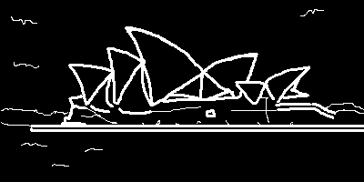
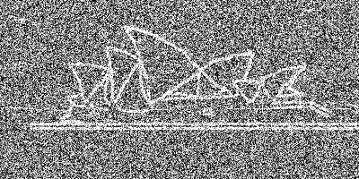
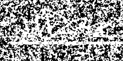
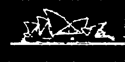
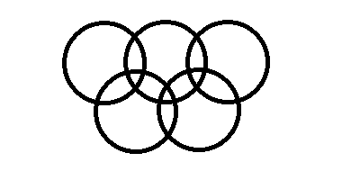
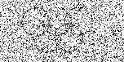
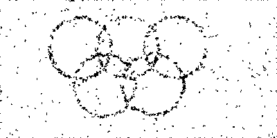
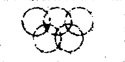
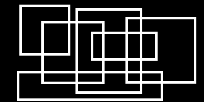
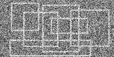
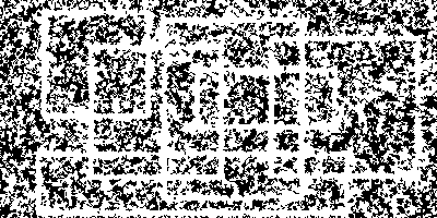
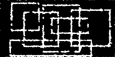
Figure 1: Example images from the binary segmentation results. From left to right, the columns are (a) the original image (b) the noisy input (c) results from Generic Cuts [2] (d) our results.

In order to evaluate our algorithms, we focused on binary denoising and interactive segmentation. For binary denoising, Generic Cuts [2] provides the most natural comparison since it is a state-of-the-art method that uses SoS priors. For interactive segmentation the natural comparison is against GrabCut [27], where we used the OpenCV implementation. We ran our general S3SVM method, which can learn an arbitrary SoS function, an also considered the special case of only using pairwise priors. For both the denoising and segmentation applications, we significantly improve on the accuracy of the hand-tuned energy functions.

5.1 Binary denoising

Our binary denoising dataset consists of a set of 20 black and white images. Each image is $400\times 200$ and either a set of geometric lines, or a hand-drawn sketch (see Figure 1). We were unable to obtain the original data used by [2], so we created our own similar data by adding independent Gaussian noise at each pixel.

For denoising, the hand-tuned Generic Cuts algorithm of [2] posed a simple MRF, with unary pixels equal to the absolute valued distance from the noisy input, and an SoS prior, where each $2\times 2$ clique penalizes the square-root of the number of edges with different labeled endpoints within that clique. There is a single parameter $\lambda$, which is the tradeoff between the unary energy and the smoothness term. The neighborhood structure $\mathcal{C}$ consists of all $2\times 2$ patches of the image.

Our learned prior includes the same unary terms and clique structure, but instead of the square-root smoothness prior, we learn a clique function $g$ to get an MRF $E_{\textrm{SVM}}(y)=\sum_{i}|y_{i}-x_{i}|+\sum_{C\in\mathcal{C}}g(y_{C})$. Note that each clique has the same energy as every other, so this is analogous to a graph cuts prior where each pairwise edge has the same attractive potential. Our energy function has 16 total parameters (one for each possible value of $g$, which is defined on $2\times 2$ patches).

We randomly divided the 20 input images into 10 training images and 10 test images. The loss function was the Hamming distance between the correct, un-noisy image and the predicted image. To hand tune the value $\lambda$, we picked the value which gave the minimum pixel-wise error on the training set. S3SVM training took only 16 minutes.

Numerically, S3SVM performed signficantly better than the hand-tuned method, with an average pixel-wise error of only 4.9% on the training set, compared to 28.6% for Generic Cuts. The time needed to do inference after training was similar for both methods: 0.82 sec/image for S3SVM vs. 0.76 sec/image for Generic Cuts. Visually, the S3SVM images are significantly cleaner looking, as shown in Figure 1.

5.2 Interactive segmentation

Input

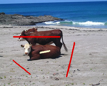
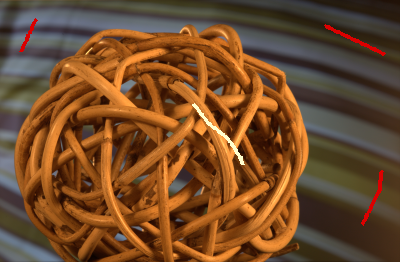
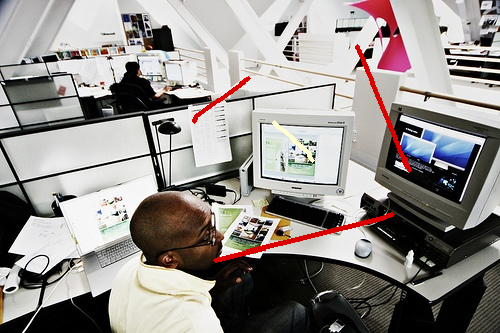
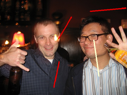
GrabCut

S3SVM-AMN

S3SVM

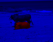
Figure 2: Example images from binary segmentation results. Input with user annotations are shown at top, with results below.

The input to interactive segmentation is a color image, together with a set of sparse foreground/background annotations provided by the user. See Figure 2 for examples. From the small set of labeled foreground and background pixels, the prediction task is to recover the ground-truth segmentation for the whole image.

Our baseline comparison is the Grabcut algorithm, which solves a pairwise CRF. The unary terms of the CRF are obtained by fitting a Gaussian Mixture Model to the histograms of pixels labeled as being definitely foreground or background. The pairwise terms are a standard contrast-sensitive Potts potential, where the cost of pixels $i$ and $j$ taking different labels is equal to $\lambda\cdot\textrm{exp}(-\beta|x_{i}-x_{j}|)$ for some hand-coded parameters $\beta,\lambda$. Our primary comparison is against the OpenCV implementation of Grabcut, available at www.opencv.org.

As a special case, our algorithm can be applied to pairwise-submodular energy functions, for which it solves the same optimization problem as in Associative Markov Networks (AMN’s) [30, 1]. Automatically learning parameters allows us to add a large number of learned unary features to the CRF.

As a result, in addition to the smoothness parameter $\lambda$, we also learn the relative weights of approximately 400 features describing the color values near a pixel, and relative distances to the nearest labeled foreground/background pixel. Further details on these features can be found in the Supplementary Material. We refer to this method as S3SVM-AMN.

Our general S3SVM method can incorporate higher-order priors instead of just pairwise ones. In addition to the unary features used in S3SVM-AMN, we add a sum-of-submodular higher-order CRF. Each $2\times 2$ patch in the image has a learned submodular clique function. To obtain the benefits of the contrast-sensitive pairwise potentials for the higher-order case, we cluster (using $k$-means) the $x$ and $y$ gradient responses of each patch into 50 clusters, and learn one submodular potential for each cluster. Note that S3SVM automatically allows learning the entire energy function, including the clique potentials and unary potentials (which come from the data) simultaneously.

We use a standard interactive segmentation dataset from [11] of 151 images with annotations, together with pixel-level segmentations provided as ground truth. These images were randomly sorted into training, validation and testing sets, of size 75, 38 and 38 respectively. We trained both S3SVM-AMN and S3SVM on the training set for various values of the regularization parameter $c$, and picked the value $c$ which gave the best accuracy on the validation set, and report the results of that value $c$ on the test set.

The overall performance is shown in the table below. Training time is measured in seconds, and testing time in seconds per image. Our implementation, which used the submodular flow algorithm based on IBFS discussed in section 3.2, will be made freely available under the MIT license.

Algorithm	Average error	Training	Testing
Grabcut	10.6$\pm$ 1.4%	n/a	1.44
S3SVM-AMN	7.5$\pm$ 0.5%	29000	0.99
S3SVM	7.3$\pm$ 0.5%	92000	1.67

Learning and validation was performed 5 times with independently sampled training sets. The averages and standard deviations shown above are from these 5 samples.

Figure 3: A multi-label segmentation result, on data from [12]. The purple label represents vegetation, red is rhino/hippo and blue is ground. There are 7 labels in the input problem, though only 3 are present in the output we obtain on this particular image.

While our focus is on binary labeling problems, we have conducted some preliminary experiments with the multi-label version of our method described in section 4.4. A sample result is shown in figure 3, using an image taken the Corel dataset used in [12].

References

- [1] D. Anguelov, B. Taskar, V. Chatalbashev, D. Koller, D. Gupta, G. Heitz, and A. Y. Ng. Discriminative learning of Markov Random Fields for segmentation of 3D scan data. In CVPR, 2005.
- [2] C. Arora, S. Banerjee, P. Kalra, and S. N. Maheshwari. Generic cuts: an efficient algorithm for optimal inference in higher order MRF-MAP. In ECCV, 2012.
- [3] M.-F. Balcan and N. J. A. Harvey. Learning submodular functions. In STOC, 2011.
- [4] Y. Boykov and V. Kolmogorov. An experimental comparison of min-cut/max-flow algorithms for energy minimization in vision. TPAMI, 26(9), 2004.
- [5] Y. Boykov, O. Veksler, and R. Zabih. Fast approximate energy minimization via graph cuts. TPAMI, 23(11), 2001.
- [6] J. Edmonds and R. Giles. A min-max relation for submodular functions on graphs. Annals of Discrete Mathematics, 1:185–204, 1977.
- [7] T. Finley and T. Joachims. Training structural SVMs when exact inference is intractable. In ICML, 2008.
- [8] A. Fix, A. Gruber, E. Boros, and R. Zabih. A graph cut algorithm for higher-order Markov Random Fields. In ICCV, 2011.
- [9] S. Fujishige and X. Zhang. A push/relabel framework for submodular flows and its refinement for 0-1 submodular flows. Optimization, 38(2):133–154, 1996.
- [10] A. V. Goldberg, S. Hed, H. Kaplan, R. E. Tarjan, and R. F. Werneck. Maximum flows by incremental breadth-first search. In European Symposium on Algorithms, 2011.
- [11] V. Gulshan, C. Rother, A. Criminisi, A. Blake, and A. Zisserman. Geodesic star convexity for interactive image segmentation. In CVPR, 2010.
- [12] X. He, R. S. Zemel, and M. A. Carreira-Perpiñán. Multiscale conditional random fields for image labeling. In CVPR, 2004.
- [13] H. Ishikawa. Transformation of general binary MRF minimization to the first order case. TPAMI, 33(6), 2010.
- [14] T. Joachims, T. Finley, and C.-N. Yu. Cutting-plane training of structural SVMs. Machine Learning, 77(1), 2009.
- [15] P. Kohli, M. P. Kumar, and P. H. Torr. P3 and beyond: Move making algorithms for solving higher order functions. TPAMI, 31(9), 2008.
- [16] P. Kohli, L. Ladicky, and P. Torr. Robust higher order potentials for enforcing label consistency. IJCV, 82, 2009.
- [17] V. Kolmogorov. Minimizing a sum of submodular functions. Discrete Appl. Math., 160(15):2246–2258, Oct. 2012.
- [18] V. Kolmogorov and R. Zabih. What energy functions can be minimized via graph cuts? TPAMI, 26(2), 2004.
- [19] H. Koppula, A. Anand, T. Joachims, and A. Saxena. Semantic labeling of 3D point clouds for indoor scenes. In NIPS, 2011.
- [20] V. Kwatra, A. Schodl, I. Essa, G. Turk, and A. Bobick. Graphcut textures: Image and video synthesis using graph cuts. SIGGRAPH, 2003.
- [21] L. Ladicky, C. Russell, P. Kohli, and P. H. S. Torr. Associative hierarchical CRFs for object class image segmentation. In ICCV, 2009.
- [22] J. Lafferty, A. McCallum, and F. Pereira. Conditional random fields: Probabilistic models for segmenting and labeling sequence data. In ICML, 2001.
- [23] H. Lin and J. Bilmes. Learning mixtures of submodular shells with application to document summarization. In UAI, 2012.
- [24] D. Munoz, J. A. Bagnell, N. Vandapel, and M. Hebert. Contextual classification with functional max-margin Markov networks. In CVPR, 2009.
- [25] J. B. Orlin. A faster strongly polynomial time algorithm for submodular function minimization. Math. Program., 118(2):237–251, Jan. 2009.
- [26] S, Roth and M, Black. Fields of experts. IJCV, 82, 2009.
- [27] C. Rother, V. Kolmogorov, and A. Blake. “GrabCut” - interactive foreground extraction using iterated graph cuts. SIGGRAPH, 23(3):309–314, 2004.
- [28] R. Sipos, P. Shivaswamy, and T. Joachims. Large-margin learning of submodular summarization models. In EACL, 2012.
- [29] M. Szummer, P. Kohli, and D. Hoiem. Learning CRFs using graph cuts. In ECCV, 2008.
- [30] B. Taskar, V. Chatalbashev, and D. Koller. Learning associative markov networks. In ICML, 2004.
- [31] B. Taskar, V. Chatalbashev, and D. Koller. Learning associative markov networks. In ICML. ACM, 2004.
- [32] B. Taskar, C. Guestrin, and D. Koller. Maximum-margin markov networks. In NIPS, 2003.
- [33] I. Tsochantaridis, T. Hofmann, T. Joachims, and Y. Altun. Support vector machine learning for interdependent and structured output spaces. In ICML, 2004.
- [34] Y. Yue and T. Joachims. Predicting diverse subsets using structural SVMs. In ICML, 2008.