Strong-field ionization of He by elliptically polarized light in attoclock configuration

Abstract

We perform time-dependent calculations of strong-field ionization of He by elliptically polarized light in configuration of recent attoclock measurements of Boge et al [PRL 111, 103003 (2013)]. By solving a 3D time-dependent Schrödinger equation, we obtain the angular offset $\theta_{m}$ of the maximum in the photoelectron momentum distribution in the polarization plane relative to the position predicted by the strong field approximation. This offset is used in attoclock measurements to extract the tunneling time. Our calculations clearly support the set of experimental angular offset values obtained with the use of non-adiabatic calibration of the in situ field intensity, and disagree with an alternative set calibrated adiabatically. These findings are in contrast with the conclusions of Boge et al who found a qualitative agreement of their semiclassical calculations with the adiabatic set of experimental data. This controversy may complicate interpretation of the recent atto-clock measurements.

One of recent advances of attosecond science was experimental observation of the time delay of photoemission after subjecting an atom to a short and intense laser pulse. Theoretical interpretation of such measurements depends on the Keldysh parameter $\gamma$ which draws the borderline between the truly quantum multiphoton regime $\gamma>1$ and a semi-classical tunneling regime $\gamma<1$ Keldysh (1965). The time delay measurements in the multi-photon regime by attosecond streaking Schultze et al. (2010) or two-photon sideband interference Klünder et al. (2011); Guénot et al. (2012) can be conveniently interpreted by the Wigner time delay theory de Carvalho and Nussenzveig (2002). Even though some quantitative differences remain between measured and calculated time delays (see e.g. Kheifets (2013)), qualitatively, these measurements are now well understood. At the same time, interpretation of the attosecond measurements in the tunneling regime by attosecond angular streaking Eckle et al. (2008a, 2008) or high harmonics generation Shafir et al. (2012) is less straightforward. Indeed, the timing of the tunneling process has been a subject of numerous discussions and a long controversy (see Landauer and Martin (1994) for a comprehensive review).

The attosecond angular streaking technique, termed colloquially as a tunneling clock or an atto-clock, uses the rotating electric-field vector of the elliptically polarized pulse to deflect photo-ionized electrons in the angular spatial direction. Then the instant of ionization is mapped to the final angle of the momentum vector in the polarization plane, and a tunneling time is calculated using a semiclassical propagation model. By employing this technique, Eckle et al. (2008) placed an intensity-averaged upper limit of 12 as on tunneling time in strong field ionization of He with peak intensities ranging from 2.3 to 3.5 units of $\rm 10^{14}~{}W/cm^{2}$. In a subsequent paper by the same group Pfeiffer et al. (2012a), the attoclock was used to obtain information on the electron tunneling geometry and to confirm vanishing tunneling time. In addition, by comparing the angular streaking results in Ar and He, multi-electron effects were clearly identified. Further on, the influence of the ion potential on the departing electron was considered and explained within a semiclassical model Pfeiffer et al. (2012b); Hofmann et al. (2013). In a recent development Weger et al. (2013), the attoclock technique was transferred from a cold-target recoil-ion momentum spectrometer (coltrims) to a velocity map imaging spectrometer (vmis). These refined attoclock measurements revealed a real and not instantaneous tunneling time over a large intensity regime Landsman et al. (2013). Various competing theories of tunneling ionization were assessed against these experimental data, and some of them were found consistent with the data.

In the latest report Boge et al. (2013), the attoclock measurements on He were used to assess the influence of non-adiabatic tunneling effects. In the tunneling regime, the electron tunnels adiabatically, it experiences a static field while tunneling and exits the tunnel with zero momentum Keldysh (1965). By employing both the coltrims and vmis techniques, the attoclock measurements of Ref. Boge et al. (2013) were extended over a large range of intensities from 1 to 8 units of $10^{14}~{}\rm W/cm^{2}$, corresponding to a variation of the Keldysh parameter $\gamma$ from 0.7 to 2.5. The upper end of the $\gamma$ interval clearly trespasses on the multiphoton regime where the adiabatic hypothesis becomes questionable and the electron exits the tunnel with a non-zero momentum. Because this exit momentum is used as a tool for in situ calibration of the field intensity in the attoclock experiments, adopting either of the adiabatic or non-adiabatic tunneling hypothesis would affect strongly the intensity calibration and the tunneling time results. In order to overcome this uncertainty, Boge et al. (2013) performed a measurement of the angle of the photoelectron momentum at the detector defined by $\theta_{m}=\arctan(p_{x~{}\rm final}/p_{y~{}\rm final})$. Provided the electron is tunnel ionized at the maximum of the electric field $E_{x}$ and is driven to the detector by the laser pulse, its final momentum is aligned with the vector potential at the moment of ionization $A_{y}$ and hence $\theta_{m}=0$. Non-zero values $\theta_{m}\neq 0$ can be attributed to the Coulomb field of the ionic core and/or a finite tunneling time

Boge et al. (2013) obtained two sets of the offset angles $\theta_{m}$ under the two tunneling scenarios. Then they attempted to reproduce their data qualitatively with a TIPIS model (Tunnel Ionization in Parabolic coordinates with Induced dipole and Stark shift). The version of the model based on the non-adiabatic tunneling hypothesis predicted increasing of the offset angle with increase of the field intensity. Conversely, the adiabatic model showed decrease of the offset with growing intensity, which was indeed the case experimentally. On this qualitative basis, Boge et al. (2013) concluded that their experiments conformed to the adiabatic tunneling scenario. Quantitative difference of the adiabatic experimental data and theory was attributed to a finite tunneling time. Comparable difference between the non-adiabatic TIPIS theory and experiment can also be attributed to the same finite tunneling time effect Cirelli, C. and Boge, R. (2013).

In the present work, we perform accurate numerical calculations of the angular offset $\theta_{m}$ by solving a 3D time-dependent Schrödinger equation (TDSE). Our theoretical model is fully ab initio, it uses no adjustable parameters and does not require any specific tunneling hypothesis. Results of our calculations support the set of experimental data calibrated under the non-adiabatic hypothesis. If this agreement is not accidental, it may indicate the influence of non-adiabatic effects predicted by the analytical theory Yudin and Ivanov (2001). It may also raise a question of validity of the TIPIS model and, more broadly, the interpretation of the tunneling time measurements reported in Landsman et al. (2013). Indeed, our numerical results, the TIPIS model predictions and the experimental data of Boge et al. (2013) are mutually contradictory. The adiabatic tunneling scenario leads to the experimental data calibration which contradicts to the present calculation. The non-adiabatic scenario leads to the TIPIS model prediction which is qualitatively incompatible with the experiment. One of the components of this triad, formed by the two theories and the experiment, is likely to be at fault.

Because of this important implication, we made every effort possible to verify our theoretical model and to validate our numerical computations. We tested the gauge invariance, partial wave and radial box convergence and the carrier envelope phase (CEP) as well as the pulse length effects. All these tests were performed successfully.

We solve the TDSE for a helium atom described in a single active electron approximation:

$$i{\partial\Psi({\bm{r}})/\partial t}=\left[\hat{H}_{\rm atom}+\hat{H}_{\rm int}(t)\right]\Psi({\bm{r}})\ ,$$ (1)

where $\hat{H}_{\rm atom}$ is the Hamiltonian of the field-free atom with effective one-electron potentials Sarsa et al. (2004); Green et al. (1969). Two different model potentials were employed and produced indistinguishable results, which assured the accuracy of the calculation. The Hamiltonian $\hat{H}_{\rm int}(t)$ describes the interaction with the EM field. For this operator we can use both the length and velocity gauges:

$$\hat{H}_{\rm int}(t)=\left\{\begin{array}[]{ccc}{\bm{E}}(t)\cdot\hat{\bm{r}}\\ {\bm{A}}(t)\cdot\hat{\bm{p}}&,\ \ {\bm{A}(t)}=-\int_{-T_{1}/2}^{t}{\bm{E}(\tau)}\ d\tau\\ \end{array}\right.$$ (2)

The field is elliptically polarized in the $xy$ plane with the components:

$$E_{x}={{\cal E}f(t)\over\sqrt{1+\epsilon^{2}}}\cos(\omega t+\phi)\ ,\ E_{y}={\epsilon{\cal E}f(t)\over\sqrt{1+\epsilon^{2}}}\sin(\omega t+\phi)$$ (3)

Here the ellipticity parameter $\epsilon=0.87$ and the carrier frequency $\omega=1.69$ eV (corresponding the wavelength $\lambda=735$ nm) are the same as in the experimental work Landsman et al. (2013). The pulse envelope was chosen to be $f(t)=\sin^{2}\pi t/T_{1}$, where $T_{1}=6T$ was the total pulse duration ($T=2\pi/\omega$ is an optical period corresponding to the carrier frequency), and $\phi$ the CEP. The bulk of calculations was performed with $\phi=0$ with a well-defined maximum of the vector potential relative to which the angular offset is measured. The electric field $\bm{E}$ and the vector potential $\bm{A}$ of this pulse are shown in Figure 1. Some calculations at few selected field intensities were performed with varying $\phi$. We also performed a separate set of calculations at varying field intensity for a shorter pulse with $T_{1}=3T$.

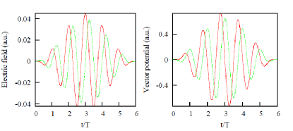
Figure 1: (Color online) The electric field (left) and the vector potential (right) of the laser pulse with $\phi=0$. Solid (red) line: $x$-components, dashed (green): $y$-components.

We seek a solution of Eq. (1) in the form of a partial wave expansion

$$\Psi({\bm{r}},t)=\sum\limits_{l=0}^{L_{\max}}\sum\limits_{\mu=-l}^{l}f_{l\mu}(r,t)Y_{l\mu}(\theta,\phi)\ ,$$ (4)

The radial part of the TDSE is discretized on a spatial grid in a box. To propagate the wave function (4) in time, we use the matrix iteration method developed in Nurhuda and Faisal (1999a) and further tested in calculations of strong field ionization driven by linear Grum-Grzhimailo et al (2010); Ivanov (2011) and circularly polarized Ivanov and Kheifets (2013) radiation.

By projecting the solution of the TDSE at the end of the laser pulse at $t=T_{1}$ on the set of the ingoing scattering states:

$$\psi^{(-)}_{{\bm{k}}}({\bm{r}})=\sum\limits_{l\mu}i^{l}e^{-i\delta_{l}}Y^{*}_{l\mu}({\bm{n}}_{{\bm{k}}})Y_{l\mu}({\bm{n}}_{{\bm{r}}})R_{kl}(r)\ ,$$ (5)

(here ${\bm{n}}_{{\bm{k}}}={\bm{k}}/k$, and ${\bm{n}}_{{\bm{r}}}={\bm{r}}/r$ are unit vectors in the direction of ${\bm{k}}$ and ${\bm{r}}$, respectively) we obtain ionization amplitudes and the electron momentum distribution:

$$P({{\bm{k}}})=|\langle\psi^{(-)}_{{\bm{k}}}|\Psi(T_{1})\rangle|^{2}$$ (6)

For the field parameters that we considered, the ionization probabilities are extremely small (of the order of $10^{-10}$) which required highly accurate computations. The issue of convergence and accuracy of the results was, therefore, critical for us in the present work. We found that convergence with respect to the number of partial waves retained in Eq. (4) is much faster in the velocity (V) gauge for the operator of the atom-field interaction (2). In the V-gauge, a convergence on the acceptable level of accuracy was achieved for $L_{\max}=40$ (laser intensity of $1.25\times 10^{14}$ W/cm² or less), $L_{\max}=50$ for the intensity of $1.5\times 10^{14}$ W/cm², $L_{\max}=60$ for the intensities in the range $1.75\times 10^{14}-2.25\times 10^{14}$ W/cm², and $L_{\max}=70$ for higher intensities. In comparison, for the intensity of $1.25\times 10^{14}$ W/cm², the L-gauge results begin to converge for $L_{\rm max}$ as large as 60. This made use of the L-gauge for higher field intensities prohibitively expensive. Results reported below, therefore, have been obtained using the V-gauge. Typical calculation required several hundred hours of CPU time, which was only possible by making our code run in parallel on a 1.2 petaflop supercomputer. A series of checks was performed to insure convergence both with respect to the parameter $L_{\rm max}$, time integration stepsize $\Delta t$ and the box size $R_{\rm max}$. Some results of these checks are illustrated in Table I for the field intensity of $1.25\times 10^{14}$ W/cm². These checks allowed us to estimate the error margin of our calculation as one degree.

Table 1: Convergence with respect to the parameter $L_{\rm max}$ and the time integration stepsize $\Delta t$ for the field intensity of $1.25\times 10^{14}$ W/cm², $T_{1}=3T$ and $\phi=0$.

Computation parameters			Ionization probability
Gauge	$L_{\rm max}$	$\Delta t$, a.u	$10^{-10}$
V	40	0.01	1.0235
V	50	0.01	1.0115
V	40	0.0075	1.0234
L	50	0.01	0.807
L	60	0.01	0.959

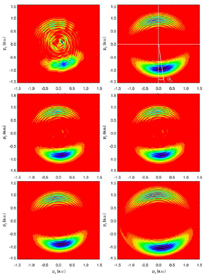
Figure 2: (Color online) Photoelectron momentum distribution in the polarization plane for the field intensities of 1, 1.25 and 1.5 units of $10^{14}$ W/cm² (left set of panels, from top to bottom) and 1.75, 2, and 2.25 units of $10^{14}$ W/cm² (right set of panels, from top to bottom), $T_{1}=6T$, $\phi=0$. The offset angle $\theta_{m}$ relative to the vertical $-p_{y}$ direction is visualized on the top right panel.

By using the projection operation (6), we calculate the electron momentum distribution in the polarization $xy$-plane. These distributions are shown in Figure 2 for the field intensities varying from $1\times 10^{14}$ to $2.25\times 10^{14}$ W/cm². Distributions were computed on a dense momenta grid in the $p_{x}p_{y}$ plane using the polar coordinates $p$ and $\theta_{p}$. To find the angular maximum $\theta_{m}$, we integrated the momentum distribution over $p$ and analyzed resulting one-dimensional angular distribution. These distributions for varying field intensities are shown in Figure 3. A similar procedure was followed in atto-clock experiments.

The well-known strong field approximation (SFA) Perelomov and Popov (1967) predicts that the direction of the maximum of the momentum distribution in the polarization plane should coincide with the direction of the vector potential $-\bm{A}(t_{0})$ at the moment $t_{0}$ when the maximum field strength is attained. For the pulse with $T_{1}=6T$ and $\phi=0$, $t_{0}=3T$ which is the midpoint of the laser pulse. The vector potential at this moment of time has zero $x$ and positive $y$ components (see the right panel of Figure 1). The SFA predicts, therefore the zero offset angle $\theta_{m}=0$ from the vertical $-p_{y}$ direction. Our TDSE calculations predict a noticeable offset $\theta_{m}$ relative to this direction which is visualized on the top right panel of Figure 2.

For the laser intensity $1\times 10^{14}$ W/cm² (the left top panel of Figure 2), one can still discern the structures in the momentum distribution reminiscent of the multiphoton regime. Nevertheless, the prominent global maximum predicted by the SFA is clearly visible. This maximum takes over completely at higher field intensities. Each multiphoton rings visible in Figure 2 corresponds to an integer number of photons absorbed by the He atom $p_{x}^{2}+p_{y}^{2}=n\omega-24.6~{}{\rm eV}$ As we project the calculated 3D momentum distribution onto the $p_{x},p_{y}$ plane, we set $p_{z}=0$. The multiphoton rings are not observed in the experiment, most probably because of the finite range of $p_{z}$ detected. Also, the experimental momentum distributions Pfeiffer et al. (2012a) show two symmetric lobes in the electron momentum distribution whereas our calculations with $\phi=0$ show two lobes of unequal strength. This asymmetry is due to the CEP variation investigated in Eckle et al. (2008a, 2008) but not controlled in the later measurements Pfeiffer et al. (2012a); Boge et al. (2013). We illustrate this asymmetry in Figure 4 where we plot the $p$-integrated momentum distributions as functions of the angle $\theta_{p}$ for various CEP values. The relative intensity of the lobes in the second and fourth quadrants is changing with $\phi$ in exactly the same manner as observed in Eckle et al. (2008a, 2008). The figure shows some drift of the angular maximum position $\theta_{m}$ with $\phi$. This is due to the drift of the direction of the vector potential at the maximum field strength, which is located at $t_{0}=3T$ when $\phi=0$ but varies slightly for other $\phi$ values. When the angular maximum values $\theta_{m}$ are compensated for this drift, they are all located at the same value (9 degrees) irrespective of $\phi$.

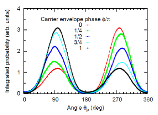
Figure 3: (Color online) The radial $p$-integrated momentum distributions as the functions of the angle $\theta_{p}$ for field intensities of 1, 1.25, 1.5, 1.75 and 2 units of $10^{14}$ W/cm². The CEP $\phi=0$, pulse duration $T_{1}=6T$.

Figure 4: (Color online) The radial $p$-integrated momentum distributions as the functions of the angle $\theta_{p}$ for CEP values $\phi=0$, $\pi/4$, $\pi/2$, $3\pi/4$ and $\pi$. Field intensity $1.5\times 10^{14}$ W/cm².

The offset from the SFA prediction $\theta_{m}=0$ can be represented in the notations of Landsman et al. (2013) as $\theta_{m}=\theta_{\rm Coul}+\omega\tau\ .$ Here $\tau$ is the tunneling time, the angle $\theta_{\rm Coul}$ arises from the effect of the ionic potential Madsen et al. (2007) which is neglected in the SFA. The TIPIS model was used in the atto-clock measurements Pfeiffer et al. (2012a); Boge et al. (2013) to evaluate the Coulomb contribution $\theta_{\rm Coul}$ and thus to evaluate the tunneling time $\tau$.

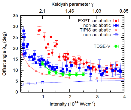
Figure 5: (Color online) The offset angle $\theta_{m}$ of the photoelectron angular distribution from which the tunneling time is extracted. The two sets of the experimental data of Boge et al. (2013) corresponding to the adiabatic and non-adiabatic field calibration are shown with the red filled circles and blue filled squares, respectively. The two analogous sets of the TIPIS calculations are shown with the red asterisks and blue open squares, respectively. The present TDSE results are shown with the green filled circles.

Our numerical results for the angular offset $\theta_{m}$, derived from Figure 3 are shown in Figure 5. In the same figure, we display two sets of the experimental data of Boge et al. (2013) and their calculations using the semi-classical TIPIS model. Each set corresponds to either adiabatic or non-adiabatic in situ calibration of the field intensity. We see clearly that our TDSE calculations favor the set of experimental data calibrated non-adiabatically and strongly disagree with an alternative set of data calibrated adiabatically. At the same time, neither of the TIPIS calculations agree with the corresponding set of the experimental data. The adiabatic TIPIS set behaves qualitatively similar to the corresponding set of the experimental data, but numerically is much closer to the non-adiabatic set of the experimental. The non-adiabatic TIPIS set is qualitatively different as it predicts the offset $\theta_{m}$ rising with an increasing field intensity.

If the agreement of the present calculation with the set of experimental offset angles, corresponding to the non-adiabatic calibration of the in situ field intensity, is not coincidental than we can draw the following conclusions: (i) non-adiabatic tunneling effects are noticeable and cannot be discarded and/or (ii) TIPIS model is inaccurate and cannot be used to extract the tunneling time. The second conclusion has a strong implication for the ongoing tunneling time debate.

The authors wish to thank Claudio Cirelli and Robert Boge for their detailed and extensive comment on the present work. Many discussions with Misha Ivanov, Olga Smirnova and Alexandra Landsman were also very useful and stimulating. The authors acknowledge support of the Australian Research Council in the form of the Discovery grant DP120101805. Resources of the National Computational Infrastructure (NCI) Facility were employed.

References

- Keldysh (1965) L. V. Keldysh, Sov. Phys. JETP 20, 1307 (1965)
- Schultze et al. (2010) M. Schultze et al., Science 328, 1658 (2010).
- Klünder et al. (2011) K. Klünder et al., Phys. Rev. Lett. 106, 143002 (2011).
- Guénot et al. (2012) D. Guénot et al., Phys. Rev. A 85, 053424 (2012).
- de Carvalho and Nussenzveig (2002) C. A. A. de Carvalho and H. M. Nussenzveig, Phys. Rep. 364, 83 (2002).
- Kheifets (2013) A. S. Kheifets, Phys. Rev. A 87, 063404 (2013)
- Eckle et al. (2008a) P. Eckle et al., Nature Phys. 4, 565 (2008a).
- Eckle et al. (2008) P. Eckle et al., Science 322, 1525 (2008).
- Shafir et al. (2012) D. Shafir et al., Nature 485, 343 (2012).
- Lein (2012) M. Lein, Nature 485, 313 (2012).
- Landauer and Martin (1994) R. Landauer and T. Martin, Rev. Mod. Phys. 66, 217 (1994).
- Pfeiffer et al. (2012a) A. N. Pfeiffer et al., Nature Phys. 8, 76 (2012a).
- Pfeiffer et al. (2012b) A. N. Pfeiffer et al., Phys. Rev. Lett. 109, 083002 (2012b).
- Hofmann et al. (2013) C. Hofmann, A. S. Landsman, C. Cirelli, A. N. Pfeiffer, and U. Keller, J. Phys. B 46, 125601 (2013).
- Weger et al. (2013) M. Weger et al., ArXiv e-prints eprint 1306.6280 (2013).
- Landsman et al. (2013) A. Landsman et al., ArXiv e-prints eprint 1301.2766 (2013).
- Boge et al. (2013) R. Boge et al., Phys. Rev. Lett. 111, 103003 (2013).
- Cirelli, C. and Boge, R. (2013) C. Cirelli and R. Boge (2013), private communication.
- Yudin and Ivanov (2001) G. L. Yudin and M. Y. Ivanov, Phys. Rev. A 64, 013409 (2001).
- Sarsa et al. (2004) A. Sarsa, F. J. Gálvez, and E. Buendia, Atomic Data and Nuclear Data Tables 88, 163 (2004).
- Green et al. (1969) A. E. S. Green, D. L. Sellin, and A. S. Zachor, Phys. Rev. 184, 1 (1969).
- Nurhuda and Faisal (1999a) M. Nurhuda and F. H. M. Faisal, Phys. Rev. A 60, 3125 (1999a).
- Grum-Grzhimailo et al (2010) A. N. Grum-Grzhimailo et al, Phys. Rev. A 81, 043408 (2010).
- Ivanov (2011) I. A. Ivanov, Phys. Rev. A 83, 023421 (2011).
- Ivanov and Kheifets (2013) I. A. Ivanov and A. S. Kheifets, Phys. Rev. A 87, 033407 (2013).
- Nurhuda and Faisal (1999b) M. Nurhuda and F. H. M. Faisal, Phys. Rev. A 60, 3125 (1999b).
- Perelomov and Popov (1967) A. M. Perelomov and V. S. Popov, Sov. Phys. JETP 25, 336 (1967).
- Madsen et al. (2007) L. B. Madsen, L. A. A. Nikolopoulos, T. K. Kjeldsen, and J. Fernández, Phys. Rev. A 76, 063407 (2007).