Restarted inverse Born series for the
Schrödinger problem with
discrete internal measurements

Abstract

Convergence and stability results for the inverse Born series [Moskow and Schotland, Inverse Problems, 24:065005, 2008] are generalized to mappings between Banach spaces. We show that by restarting the inverse Born series one obtains a class of iterative methods containing the Gauss-Newton and Chebyshev-Halley methods. We use the generalized inverse Born series results to show convergence of the inverse Born series for the Schrödinger problem with discrete internal measurements. In this problem, the Schrödinger potential is to be recovered from a few measurements of solutions to the Schrödinger equation resulting from a few different source terms. An application of this method to a problem related to transient hydraulic tomography is given, where the source terms model injection and measurement wells.

1 Introduction

We consider the problem of finding a Schrödinger potential $q(\mathbf{x})$ (which may be complex) from discrete internal measurements of the solution $u_{i}(\mathbf{x})$ to the Schrödinger equation

$$\left\{\begin{aligned} -\Delta u_{i}+qu_{i}&=\phi_{i},&&\text{ for }\mathbf{x}\in\Omega,\\ u_{i}&=0,&&\text{ for }\mathbf{x}\in\partial\Omega,\end{aligned}\right.$$ (1)

in a closed bounded set $\Omega\subset\mathbb{R}^{d}$ for $d\geq 2$, and for different (known) source terms $\phi_{i}\in C^{\infty}(\Omega)$, $i=1,\ldots,N$. We further assume $q\in L^{\infty}(\Omega)$ is known in $\Omega\backslash\widetilde{\Omega}$, where $\widetilde{\Omega}$ is a closed subset of $\Omega$ with a finite distance separating $\partial\widetilde{\Omega}$ and $\partial\Omega$.

The internal measurements we consider are of the form

$$D_{i,j}=\int_{\Omega}\phi_{j}(\mathbf{x})u_{i}(\mathbf{x})d\mathbf{x},\text{for $i,j=1,\ldots,N$}.$$ (2)

The measurement $D_{i,j}$ is a weighted average of the field $u_{i}$ resulting from the $i-$th source term. Although it is not necessary for our method to work, we assume for simplicity the same source terms are used as weights for the averages.

A motivation for this inverse Schrödinger problem is transient hydraulic tomography (see e.g. [4] for a review). The hydraulic pressure or head $v(\mathbf{x},t)$ in an underground reservoir or aquifer $\Omega$ resulting from a source $\psi(\mathbf{x},t)$ (the injection well) satisfies the initial value problem

$$\left\{\begin{aligned} Sv_{t}&=\nabla\cdot(\sigma\nabla v)-\psi,&&\text{ for }\mathbf{x}\in\Omega,~{}t>0,\\ v(\mathbf{x},t)&=0,&&\text{ for }\mathbf{x}\in\partial\Omega,~{}t>0,\\ v(\mathbf{x},0)&=g(\mathbf{x}),&&\text{ for }\mathbf{x}\in\Omega.\end{aligned}\right.$$ (3)

Here $S(\mathbf{x})$ is the storage coefficient and $\sigma(\mathbf{x})$ the hydraulic conductivity of the aquifer. The inverse problem is to image both $S(\mathbf{x})$ and $\sigma(\mathbf{x})$ from a series of measurements made by fixing a source term at one well, and measuring the resulting pressure response at the other wells. We show in section 6 that the inverse problem of reconstructing $S(\mathbf{x})$ and $\sigma(\mathbf{x})$ from these sparse (and discrete) internal pressure measurements, can be recast as an inverse Schrödinger problem with discrete measurements as in (2).

The main tool we use here for solving the inverse Schrödinger problem is inverse Born series. Inverse Born series have been used to solve inverse problems in different contexts such as optical tomography [10, 9, 12, 11], the Calderón or electrical impedance tomography problem [1] and in inverse scattering for the wave equation [8].

In section 2 we generalize the inverse Born series convergence results of Moskow and Schotland [11] and Arridge et al. [1], to nonlinear mappings between Banach spaces. The convergence results of inverse Born series in this generalized setting are given in section 2.3 and proved in A, following the same pattern of the proofs in [11, 1]. This new framework is applied in section 3 to a few problems that have been solved before with inverse Born series. We also show that both forward and inverse Born series are closely related to Taylor series. Since the cost of calculating the $n-$th term in an inverse Born series grows exponentially with $n$, we restart it after having computed a few $k$ terms (i.e. we truncate the series to $k$ terms and iterate). We show in section 4 that restarting the inverse Born series gives a class of iterative methods that includes the Gauss-Newton and Chebyshev-Halley methods. For the discrete measurements Schrödinger problem, we prove that the necessary conditions for convergence of the inverse Born series are satisfied (section 5). Then in section 6, we explain how the transient hydraulic tomography problem can be transformed into a discrete measurement Schrödinger problem. Finally in section 7 we present numerical experiments comparing the performance of inverse Born series with other iterative methods and their effectiveness for reconstructing the Schrödinger potential in (1) and for solving the transient hydraulic tomography problem. We conclude in section 8 with a summary of our main results.

2 Forward and inverse Born series in Banach spaces

We start by extending the notion of Born series and inverse Born series [10, 11] to operators between Banach spaces. The idea being to give a common framework for the convergence proofs of the inverse Born series for diffuse waves [11], the Calderón problem [1] and the discrete internal measurements Schrödinger problem. This generalization also highlights that the inverse Born series are a systematic way of finding non-linear approximate inverses for non-linear mappings. The resulting approximate inverses are valid locally and have guaranteed error estimates.

In sections 2.1 and 2.2 we define forward and inverse Born series for a mapping $f$ from a Banach space $X$ (the parameter space) to another Banach space $Y$ (the data space). Then in section 2.3 we state local convergence results for inverse Born series in Banach spaces that are valid under mild assumptions on the forward Born series. The proofs are included in the A as they are patterned after the proofs in [11, 1]. Examples of forward and inverse Born series are included in section 3.

2.1 Forward Born series

Let $X$ and $Y$ be Banach spaces and consider a mapping $f:X\to Y$. In inverse problems applications $X$ is typically the parameter space and $Y$ the data or measurements space. The forward problem is to find the measurements $y=f(x)$ from known parameters $x$. The inverse problem is to estimate the parameters $x$ knowing the measurements $y$.

Born series involve operators in $\mathcal{L}(X^{\otimes n},Y)$, i.e. bounded linear operators from $X^{\otimes n}$ to $Y$. Here tensor products are used to define the Banach space

$$X^{\otimes n}=\underbrace{X\otimes\cdots\otimes X}_{\text{$n$ times}},$$

endowed with the norm

$$\|x_{1}\otimes\cdots\otimes x_{n}\|_{X^{\otimes n}}=\|x_{1}\|_{X}\cdot\cdots\cdot\|x_{n}\|_{X}.$$ (4)

Notice that a map $a\in\mathcal{L}(X^{\otimes n},Y)$ can be identified to a bounded multilinear (or $n-$linear) map $\widetilde{a}:X^{n}\to Y$ defined by:

$$\widetilde{a}(x_{1},\ldots,x_{n})=a(x_{1}\otimes\cdots\otimes x_{n}).$$

Forward Born series express the measurements for a parameter $x+h\in X$ near a known parameter $x\in X$, assuming knowledge of $y=f(x)$.

Definition 1.

A nonlinear map $f:X\to Y$ admits a Born series expansion at $x\in X$ if there are are bounded linear operators $a_{n}\in\mathcal{L}(X^{\otimes n},Y)$ (possibly depending on $x$) such that

$$d(h)=f(x+h)-f(x)=\sum_{n=1}^{\infty}a_{n}(h^{\otimes n}),$$ (5)

and the $a_{n}$ satisfy the bound

$$\|a_{n}\|\leq\alpha\mu^{n}~{}\text{for $n=0,1,\ldots$}.$$ (6)

It follows from the bounds on the operators $a_{n}$, that the Born series converges locally, i.e. when $h$ is sufficiently small:

$$\|h\|<1/\mu.$$ (7)

This restriction on the size of the perturbation $h$ can be thought of as the radius of convergence of the expansion about the point $x$.

2.2 Inverse Born series

The purpose of inverse Born series is to recover $h$ from knowing the difference in measurements $d(h)=f(x+h)-f(x)$ from a (known) reference combination of parameters $x$ and measurements $y=f(x)$. The original idea in [10] is to write a power series of the data $d$,

$$g(d)=\sum_{n=1}^{\infty}b_{n}(d^{\otimes n}),$$ (8)

involving the operators $b_{n}\in\mathcal{L}(Y^{\otimes n},X)$, which are obtained by requiring (formally) that $g$ is the inverse of $d(h)$, i.e. $g(d(h))=h$. By equating operators $\mathcal{L}(X^{\otimes n},Y)$ with the same tensor power $n$, the operators $b_{n}$ need to satisfy:

$$I =b_{1}(a_{1})$$ (9)

$$0 =b_{1}(a_{2})+b_{2}(a_{1}\otimes a_{1})$$

$$0 =b_{1}(a_{3})+b_{2}(a_{1}\otimes a_{2})+b_{2}(a_{2}\otimes a_{1})+b_{3}(a_{1}\otimes a_{1}\otimes a_{1})$$

$$\vdots$$

$$0 =\sum_{m=1}^{n}\sum_{s_{1}+\cdots+s_{m}=n}b_{m}(a_{s_{1}}\otimes\cdots\otimes a_{s_{m}})$$

where $I$ is the identity in the parameter space $X$. The requirement that $b_{1}a_{1}=I$ is quite strong and may not be possible, for example when the measurement space $Y$ is finite dimensional and $X$ is infinite dimensional. Nevertheless if we assume that $b_{1}$ is both a right and left inverse of $a_{1}$ we can express the operators $b_{n}$ in terms of the operators $a_{n}$ and $b_{1}$:

$$b_{2} =-b_{1}a_{2}(b_{1}\otimes b_{1})$$ (10)

$$b_{3} =-(b_{1}a_{3}+b_{2}(a_{1}\otimes a_{2})+b_{2}(a_{2}\otimes a_{1}))(b_{1}\otimes b_{1}\otimes b_{1})$$

$$\vdots$$

$$b_{n} =-\left(\sum_{m=1}^{n-1}\sum_{s_{1}+\cdots+s_{m}=n}b_{m}(a_{s_{1}}\otimes\cdots\otimes a_{s_{m}})\right)(b_{1}^{\otimes n}).$$

Since an inverse of $a_{1}$ is not necessarily available, the key is to choose $b_{1}\in\mathcal{L}(Y,X)$ as a regularized pseudoinverse of $a_{1}$ so that $b_{1}a_{1}$ is close to the identity, at least in some subspace. This allows to define the inverse Born series.

Definition 2.

Assume $f:X\to Y$ admits a Born series (Definition 1) and let $b_{1}\in\mathcal{L}(Y,X)$. The inverse Born series for $f$ using $b_{1}$ is the power series $g(d)$ given by (8) where the operators $b_{n}\in\mathcal{L}(Y^{\otimes n},X)$ are defined for $n\geq 2$ by (10). Here again we note the dependence of the operators $b_{n}$, $n\geq 2$, on the expansion point $x\in X$ and the operator $b_{1}$.

We now state results that guarantee convergence of the inverse Born series, and give an error estimate between the limit of the inverse Born series and the true parameter perturbation $h$. The error estimate involves $\|(I-b_{1}a_{1})h\|$, that is how well the operator $b_{1}a_{1}$ approximates the identity for $h$. These results require that both $h$ and $d(h)=f(x+h)-f(x)$ are sufficiently small.

2.3 Inverse Born series local convergence

Convergence and stability for the forward and inverse Born series were established by Moskow and Schotland [11] for an inverse scattering problem for diffuse waves (see also section 3.3). Specifically they obtained bounds on the operators $a_{n}$ in (27) similar to the bounds (6). With these bounds, it is possible to show convergence and stability of the inverse Born series and even give a reconstruction error bound [11].

The convergence and stability proofs in [11] for the diffuse wave problem carry out without major modifications to the general Banach space setting. We give in this section a summary of results analogous to those in [11]. The proofs are deferred to A, as they closely follow the proof pattern in [11].

The following Lemma shows that if the forward Born operators satisfy the bounds (6), the operators $b_{n}$ are also bounded under a smallness condition on the linear operator $b_{1}$ that is used to prime the inverse Born series.

Lemma 1.

Assume $f:X\to Y$ admits a Born series and that

$$\|b_{1}\|<\frac{1}{(1+\alpha)\mu},$$ (11)

where $\alpha$ and $\mu$ are as in Definition (1). Then the coefficients (10) of the inverse Born series satisfy the estimate

$$\|b_{n}\|\leq\beta((1+\alpha)\mu\|b_{1}\|)^{n},~{}\text{for $n\geq 2$}$$ (12)

where

$$\beta=\|b_{1}\|\exp\left(\frac{1}{1-(1+\alpha)\mu\|b_{1}\|}\right).$$ (13)

Convergence of the inverse Born series follows from the bounds in Lemma 1 and a smallness condition on the data $d$.

Theorem 1 (Convergence of inverse Born series).

The inverse Born series (8) induced by $b_{1}$ and associated with the forward Born series (5) converges if

$$\|b_{1}\|<\frac{1}{(1+\alpha)\mu}$$ (14)

and the data is sufficiently small

$$\|d\|<\frac{1}{(1+\alpha)\mu\|b_{1}\|}.$$ (15)

If $h_{*}$ is the limit of the series, one can estimate the error due to truncating the series by

$$\left\|h_{*}-\sum_{n=1}^{N}b_{n}(d^{\otimes n})\right\|\leq\beta\frac{((1+\alpha)\mu\|b_{1}\|\|d\|)^{N+1}}{1-(1+\alpha)\mu\|b_{1}\|\|d\|}.$$

Stability also follows using essentially the same proof as in [11].

Theorem 2 (Stability of inverse Born series).

Assume $\|b_{1}\|<((1+\alpha)\mu)^{-1}$ and that we have two data $d_{1}$ and $d_{2}$ satisfying $M=\max(\|d_{1}\|,\|d_{2}\|)<((1+\alpha)\mu\|b_{1}\|)^{-1}$. Let $h_{i}=g(d_{i})$ for $i=1,2$ (i.e. the limit of the inverse Born series). Then the reconstructions are stable with respect to perturbations in the data in the sense that:

$$\|h_{1}-h_{2}\|<C\|d_{1}-d_{2}\|,$$ (16)

where the constant $C$ depends on $M$, $\alpha$, $\mu$, and $\|b_{1}\|$.

Theorem 1 guarantees convergence of the forward and inverse Born series:

$$d=\sum_{j=1}^{\infty}a_{j}(h^{j})\quad\text{and}\quad h_{*}=\sum_{j=1}^{\infty}b_{j}(d^{j}).$$ (17)

The limit $h_{*}$ of the inverse Born series is, in general, different from the true parameter perturbation $h$. The following theorem provides an estimate of the error $\|h-h_{*}\|$.

Theorem 3 (Error estimate).

Assuming that $\|h\|\leq M$, $\|b_{1}a_{1}h\|\leq M$ with

$$M<\frac{1}{(1+\alpha)\mu},$$

and that the hypothesis of theorem 1 hold, i.e.

$$\|b_{1}\|\leq\frac{1}{(1+\alpha)\mu}~{}\text{and}~{}\|d\|\leq\frac{1}{(1+\alpha)\mu\|b_{1}\|},$$

we have the following error estimate for the reconstruction error of the inverse Born series:

$$\left\|h-\sum_{n=1}^{\infty}b_{n}(d^{n})\right\|\leq C\|(I-b_{1}a_{1})h\|,$$ (18)

where the constant $C$ depends only on $M$, $\alpha$, $\beta$ and $\mu$ and $\|b_{1}\|$.

The proofs of lemma 1, theorems 1, 2, and 3 can be found in A.

3 Examples of forward and inverse Born series

We write examples of forward and inverse Born series in the framework of section 2. We start by showing in section 3.1 that forward and inverse Born series are intimately related to Taylor series. Another example is that of Neumann series (section 3.2). We also include the forward and inverse Born series from [11, 1], namely those for the diffuse waves for optical tomography (section 3.3) and the electrical impedance tomography problem (section 3.4). We finish the examples with the discrete internal measurements Schrödinger problem (section 3.5), which is the main application of inverse Born series that we are concerned with here.

3.1 Taylor series

• Parameter space: $X=$ Banach space

• Measurement space: $Y=X$ (for simplicity)

• Forward map: $f$ analytic (see e.g. [13])

• Forward Born series coefficients: About $x\in X$, the coefficients $a_{n}$ can be any operators in $\mathcal{L}(X^{\otimes n},X)$ agreeing with $f^{(n)}(x)/n!$ on the diagonal i.e. for any $h\in X$,

  $$a_{n}(h^{\otimes n})=\frac{1}{n!}f^{(n)}(x)(h^{\otimes n}).$$

  Here $f^{(n)}$ is the $n-$th Fréchet derivative of $f$, see e.g. [14, §4.5] for a definition.

Here we use the theory of analytic functions between Banach spaces (see e.g. [13]) which assumes that the function $f$ is $C^{\infty}$ and that the Taylor series of the function

$$f(x+h)=\sum_{n=0}^{\infty}\frac{1}{n!}f^{(n)}(x)(h^{\otimes n})$$ (19)

converges absolutely and uniformly for $h$ small enough. If in addition we assume that $f$ admits a Born series expansion at $x$, then we have

$$d(h)=f(x+h)-f(x)=\sum_{n=1}^{\infty}\frac{1}{n!}f^{(n)}(x)(h^{\otimes n})=\sum_{n=1}^{\infty}a_{n}(h^{\otimes n}).$$

That is the Taylor series and Born series coefficients, $f^{(n)}(x)/n!$ and $a_{n}$ respectively, agree at the diagonal $h^{\otimes n}$.

Since $f$ is $C^{\infty}$, the Fréchet derivatives $f^{(n)}$ are symmetric in the sense that for any permutation $\pi$ of $\{1,\ldots,n\}$ we have that

$$f^{(n)}(h_{1}\otimes\cdots\otimes h_{n})=f^{(n)}(h_{\pi(1)}\otimes\cdots\otimes h_{\pi(n)}).$$

The Born series coefficients $a_{n}$ in general do not satisfy this property, however we can consider their symmetrization $\widetilde{a}_{n}:X^{\otimes n}\to Y$ defined by

$$\widetilde{a}_{n}(h_{1}\otimes\cdots\otimes h_{n})=\frac{1}{n!}\sum_{\pi}a_{n}(h_{\pi(1)}\otimes\cdots\otimes h_{\pi(n)})$$ (20)

where the summation is taken over all permutations $\pi$ of $\{1,\ldots,n\}$.

Clearly we have that

$$\widetilde{a}_{n}(h^{\otimes n})=\frac{1}{n!}\sum_{\pi}a_{n}(h^{\otimes n})=a_{n}(h^{\otimes n}),$$

and so we have the following equality:

$$d(h)=f(x+h)-f(x)=\sum_{n=1}^{\infty}\frac{1}{n!}f^{(n)}(x)(h^{\otimes n})=\sum_{n=1}^{\infty}\widetilde{a}_{n}(h^{\otimes n}).$$

We then have two analytic functions that are equal for $h$ sufficiently small, therefore the symmetric operators $\frac{1}{n!}f^{(n)}(x)$ and $\widetilde{a}_{n}$ must be identical (see [13]). Therefore the Born series and Taylor series coefficients are essentially the same, up to a symmetrization.

If $a_{1}=f^{(1)}(x)$ is invertible (this is where the assumption $X=Y$ is used), we can apply the implicit function theorem (see e.g. [13] or [14, §4.6]) to guarantee the existence of $f^{-1}$ in a neighborhood of $x$. Moreover the inverse is analytic [13] in a neighborhood of $y=f(x)$ and admits a Taylor series near $y$

$$f^{-1}(y+d)=\sum_{n=0}^{\infty}\frac{1}{n!}(f^{-1})^{(n)}(y)(d^{\otimes n}).$$ (21)

On the other hand, if $b_{1}=a_{1}^{-1}$ we can define an inverse Born series for $f$ as in (8). By the error estimate for the inverse Born series (Theorem 3) we can guarantee that $h=g(d(h))=g(f(x+h)-f(x))$ for $h$ and $d(h)$ sufficiently small. Since $f$ is invertible in a neighborhood of $y$ we can also write $g$ in terms $f^{-1}$

$$g(d)=f^{-1}(y+d)-f^{-1}(y)=f^{-1}(y+d)-x.$$

Using the Taylor series (21) for $f^{-1}$ we can write

$$g(d)=\sum_{n=1}^{\infty}b_{n}(d^{\otimes n})=\sum_{n=1}^{\infty}\frac{1}{n!}(f^{-1})^{(n)}(y)(d^{\otimes n}).$$ (22)

As is the case for the forward Born operators $a_{n}$, the inverse Born operators $b_{n}$ are in general not symmetric. If we consider their symmetrization $\widetilde{b}_{n}$ (as in (20)), then we find that the symmetric operators $\widetilde{b}_{n}$ and $\frac{1}{n!}(f^{-1})^{(n)}(y)$ are the same. Therefore inverse Born series is a way of calculating (up to a symmetrization) the Taylor series for $f^{-1}$ from the Taylor series for $f$.

3.2 Neumann series

• Parameter space: $X=\mathbb{R}^{N}$

• Measurement space: $Y=\mathbb{R}^{n\times n}$

• Forward map: $f(\mathbf{x})=\mathbf{M}^{T}(\mathbf{L}-\operatorname{diag}(\mathbf{x}))^{-1}\mathbf{M}$, where $\mathbf{L}\in\mathbb{R}^{N\times N}$ is invertible and $\mathbf{M}\in\mathbb{R}^{N\times n}$.

• Forward Born series coefficients: About $\mathbf{0}$, the coefficients are $a_{n}(\mathbf{h})=\mathbf{M}^{T}(\mathbf{L}^{-1}\operatorname{diag}(\mathbf{h}))^{n}\mathbf{L}^{-1}\mathbf{M}$.

The forward Born series in this is example comes from the Neumann series for the inverse of $\mathbf{L}-\operatorname{diag}(\mathbf{h})$, when it exists. Indeed if for some matrix induced norm $\|\mathbf{L}^{-1}\operatorname{diag}(\mathbf{h})\|<1$, this inverse exists and is given by the Neumann series

$$(\mathbf{L}-\operatorname{diag}(\mathbf{h}))^{-1}=\left(\sum_{n=0}^{\infty}(\mathbf{L}^{-1}\operatorname{diag}(\mathbf{h}))^{n}\right)\mathbf{L}^{-1}.$$ (23)

The forward Born series is then

$$f(\mathbf{h})-f(\mathbf{0}) =\mathbf{M}^{T}(\mathbf{L}-\operatorname{diag}(\mathbf{h}))^{-1}\mathbf{M}-\mathbf{M}^{T}\mathbf{L}^{-1}\mathbf{M}$$ (24)

$$=\sum_{n=1}^{\infty}\mathbf{M}^{T}(\mathbf{L}^{-1}\operatorname{diag}(\mathbf{h}))^{n}\mathbf{L}^{-1}\mathbf{M}.$$

The inverse Born series can be defined by using as $b_{1}$ a regularized pseudoinverse of the linear map $a_{1}(\mathbf{h})=\mathbf{M}^{T}\mathbf{L}^{-1}\operatorname{diag}(\mathbf{h})\mathbf{L}^{-1}\mathbf{M}$. By the convergence results of section 2.3, the inverse Born series converges under smallness conditions for $\mathbf{h}$, $f(\mathbf{h})-f(\mathbf{0})$ and $b_{1}$.

This problem is motivated by a discretization of the Schrödinger equation $\Delta u-qu=\phi$ with finite differences. The matrix $\mathbf{L}$ is the finite difference discretization of the Laplacian and $\mathbf{h}$ is the Schrödinger potential at the discretization nodes. The matrix $\mathbf{M}$ corresponds to different source terms $\phi$, which are also used to measure $u$ (collocated sources and receiver setup as the one we use for the Schrödinger problem with discrete internal measurements in section 3.5). This example can be easily modified when the discretization of the $qu$ term in the Schrödinger equation is not a diagonal matrix (as is often the case for finite elements). The collocated sources and receivers setup can be changed as well by using a matrix other than $\mathbf{M}^{T}$ in the definition of $f(\mathbf{x})$.

3.3 Optical tomography with diffuse waves model [11]

In the diffuse waves approximation for optical tomography (see e.g. [2] for a review), the energy density $G_{q}(\mathbf{x},\mathbf{y})$ resulting from a point source $\mathbf{y}\in\Omega$ satisfies a Schrödinger type equation:

$$\left\{\begin{aligned} -\Delta_{\mathbf{x}}G_{q}(\mathbf{x},\mathbf{y})+q(\mathbf{x})G_{q}(\mathbf{x},\mathbf{y})&=-\delta(\mathbf{x}-\mathbf{y}),&&\text{for $\mathbf{x}\in\Omega$,}\\ G_{q}(\mathbf{x},\mathbf{y})+\ell\mathbf{n}(\mathbf{x})\cdot\nabla_{\mathbf{x}}G_{q}(\mathbf{x},\mathbf{y})&=0,&&\text{for $\mathbf{x}\in\partial\Omega$},\end{aligned}\right.$$ (25)

where the domain $\Omega\subset\mathbb{R}^{d}$, $d\geq 2$ has a smooth boundary $\partial\Omega$, and $q(\mathbf{x})\geq 0$ is the absorption coefficient. The $\ell\geq 0$ in the Robin boundary condition is given and, as usual, $\mathbf{n}(\mathbf{x})$ denotes the unit outward pointing normal vector to $\partial\Omega$ at $\mathbf{x}$. The inverse problem here is to recover the absorption coefficient $q(\mathbf{x})$ from knowledge of $G_{q}(\mathbf{x},\mathbf{y})$ on $\partial\Omega\times\partial\Omega$. This data amounts to taking measurements of the energy density at all $\mathbf{x}\in\partial\Omega$ for all source locations $\mathbf{y}\in\partial\Omega$ or to knowing the Robin-to-Dirichlet map for $q$. If the difference between the absorption coefficient $q(\mathbf{x})$ and a known reference coefficient $q_{0}(\mathbf{x})$ is supported in some $\widetilde{\Omega}\subset\Omega$ (with $\partial\Omega$ and $\partial\widetilde{\Omega}$ separated by a finite distance), then $G_{q}$ satisfies the Lippmann-Schwinger type integral equation:

$$G_{q}(\mathbf{x},\mathbf{y})=G_{q_{0}}(\mathbf{x},\mathbf{y})+\int_{\widetilde{\Omega}}d\mathbf{z}\;G_{q_{0}}(\mathbf{x},\mathbf{z})(q(\mathbf{z})-q_{0}(\mathbf{z}))G_{q}(\mathbf{z},\mathbf{y}).$$ (26)

Moskow and Schotland [11] show that the forward Born or scattering series for this problem can be defined as follows.

• Parameter space: $X=L^{p}(\widetilde{\Omega})$ for $2\leq p\leq\infty$.

• Measurement space: $Y=L^{p}(\partial\Omega\times\partial\Omega)$

• Forward map: $f:q\to G_{q}(\mathbf{x},\mathbf{y})|_{\partial\Omega\times\partial\Omega}$.

• Forward Born series coefficients: For $\eta_{1},\ldots,\eta_{n}\in L^{p}(\widetilde{\Omega})$ and $\mathbf{x}_{1},\mathbf{x}_{2}\in\partial\Omega$, the coefficient for the Born series expansion about $q=q_{0}$ is

  $$(a_{n}(\eta_{1}\otimes\cdots\otimes\eta_{n}))(\mathbf{x}_{1},\mathbf{x}_{2})=\\ \int_{\widetilde{\Omega}^{n}}G_{q_{0}}(\mathbf{x}_{1},\mathbf{y}_{1})G_{q_{0}}(\mathbf{y}_{1},\mathbf{y}_{2})\ldots G_{q_{0}}(\mathbf{y}_{n-1},\mathbf{y}_{n})G_{q_{0}}(\mathbf{y}_{n},\mathbf{x}_{2})\\ \eta_{1}(\mathbf{y}_{1})\ldots\eta_{n}(\mathbf{y}_{n})~{}d\mathbf{y}_{1}\ldots d\mathbf{y}_{n}.$$ (27)

In particular, the results of Moskow and Schotland [11] guarantee that the operators $a_{n}$ satisfy the bounds (6) assuming $q_{0}$ is constant and that $q$ is sufficiently close to $q_{0}$. Therefore one can define an inverse Born series through the procedure (10), and this series converges under appropriate conditions (see [11] and section 2.3).

3.4 The Calderón or electrical impedance tomography problem [1]

The electric potential inside a domain $\Omega$ with positive conductivity $\sigma(\mathbf{x})\in L^{\infty}(\Omega)$ resulting from a point source located at $\mathbf{y}\in\Omega$ satisfies the equation

$$\left\{\begin{aligned} \nabla_{\mathbf{x}}\cdot[\sigma(\mathbf{x})\nabla_{\mathbf{x}}G_{\sigma}(\mathbf{x},\mathbf{y})]&=-\delta(\mathbf{x}-\mathbf{y}),&&\text{for $\mathbf{x}\in\Omega$}\\ G_{\sigma}(\mathbf{x},\mathbf{y})+z\sigma\mathbf{n}(\mathbf{x})\cdot\nabla_{\mathbf{x}}G_{\sigma}(\mathbf{x},\mathbf{y})&=0,&&\text{for $\mathbf{x}\in\partial\Omega$.}\end{aligned}\right.$$ (28)

Here we assume the contact impedance $z\geq 0$ is known and that $\sigma$ is constant on $\partial\Omega$. The domain $\Omega$ is also assumed to be in $\mathbb{R}^{d}$, $d\geq 2$ and with smooth boundary. The electric impedance tomography (EIT) problem consists in recovering the conductivity $\sigma$ from the Robin-to-Dirichlet map, i.e. from knowledge of $G_{\sigma}(\mathbf{x},\mathbf{y})$ on $\partial\Omega\times\partial\Omega$ (see e.g. [3] for a review of EIT). If the difference between $\sigma$ and a known reference conductivity $\sigma_{0}$ is supported in $\widetilde{\Omega}\subset\Omega$ (with $\partial\widetilde{\Omega}$ at a finite distance from $\partial\Omega$), $G_{\sigma}$ satisfies the integral equation

$$G_{\sigma}(\mathbf{x},\mathbf{y})=G_{\sigma_{0}}(\mathbf{x},\mathbf{y})+\int_{\widetilde{\Omega}}d\mathbf{z}\;G_{\sigma_{0}}(\mathbf{x},\mathbf{z})\nabla_{\mathbf{z}}\cdot[(\sigma(\mathbf{z})-\sigma_{0}(\mathbf{z}))\nabla_{\mathbf{z}}G_{\sigma}(\mathbf{z},\mathbf{y})].$$ (29)

Integrating by parts and using that $\sigma=\sigma_{0}$ on $\partial\Omega$, $G_{\sigma}$ obeys a Lippmann-Schwinger type equation:

$$G_{\sigma}(\mathbf{x},\mathbf{y})=G_{\sigma_{0}}(\mathbf{x},\mathbf{y})-\int_{\widetilde{\Omega}}d\mathbf{z}\;(\sigma(\mathbf{x})-\sigma_{0}(\mathbf{x}))\nabla_{\mathbf{z}}G_{\sigma_{0}}(\mathbf{x},\mathbf{z})\cdot\nabla_{\mathbf{z}}G_{\sigma}(\mathbf{z},\mathbf{y}).$$ (30)

As shown by Arridge et al. [1], one can then define a forward Born series that can be summarized as follows.

• Parameter Space: $X=L^{\infty}(\widetilde{\Omega})$.

• Measurement space: $Y=L^{\infty}(\partial\Omega\times\partial\Omega)$.

• Forward map: $f:\sigma\to G_{\sigma}(\mathbf{x},\mathbf{y})|_{\partial\Omega\times\partial\Omega}$.

• Forward Born series coefficients: For $\eta_{1},\ldots,\eta_{n}\in L^{\infty}(\widetilde{\Omega})$ and $\mathbf{x}_{1},\mathbf{x}_{2}\in\partial\Omega$, the coefficient for the Born series expansion about $\sigma=\sigma_{0}$ is

  $$a_{n}(\eta_{1}\otimes\cdots\otimes\eta_{n})(\mathbf{x}_{1},\mathbf{x}_{2})=\\ (-1)^{n}\int_{\widetilde{\Omega}}d\mathbf{y}_{1}\;\eta_{1}(\mathbf{y}_{1})\nabla_{\mathbf{y}_{1}}G_{\sigma_{0}}(\mathbf{y}_{1},\mathbf{x}_{1})\cdot\nabla_{\mathbf{y}_{1}}\int_{\widetilde{\Omega}}d\mathbf{y}_{2}\;\eta_{2}(\mathbf{y}_{2})\nabla_{\mathbf{y}_{2}}G_{\sigma_{0}}(\mathbf{y}_{2},\mathbf{y}_{1})\cdot\\ \cdots\nabla_{\mathbf{y}_{n-1}}\int_{\widetilde{\Omega}}d\mathbf{y}_{n}\;\eta_{n}(\mathbf{y}_{n})\nabla_{\mathbf{y}_{n}}G_{\sigma_{0}}(\mathbf{y}_{n},\mathbf{y}_{n-1})\cdot\nabla_{\mathbf{y}_{n}}G_{\sigma_{0}}(\mathbf{y}_{n},\mathbf{x}_{2}).$$ (31)

Arridge et al. [1] show that for $\sigma_{0}$ constant, the operators $a_{n}$ satisfy the bounds (6) and so an inverse Born series can be defined following the procedure (10). The convergence of this series is established in [1] and can also be shown using the generalization in section 2.3.

3.5 The Schrödinger problem with discrete internal measurements

Instead of having infinitely many measurements as in the optical tomography inverse Schrödinger problem (outlined in section 3.3), we consider here the case where we only have access to finitely many internal measurements $D_{i,j}$ (see equation (2)) of the fields $u_{i}$, $i=1,\ldots,N$, satisfying (1). We also allow the Schrödinger potential in (1) to be complex (as discussed in section 6, this is useful when solving the transient hydraulic tomography problem).

The Green function $G_{q}(\mathbf{x},\mathbf{y})$ for the problem (1) satisfies (25) with homogeneous Dirichlet boundary conditions (instead of homogeneous Robin boundary conditions). The fields $u_{i}$ can be expressed in terms of the Green function $G_{q}$ as

$$u_{i}(\mathbf{x})=-\int_{\Omega}d\mathbf{y}\;G_{q}(\mathbf{x},\mathbf{y})\phi_{i}(\mathbf{y}),~{}i=1,\ldots,N.$$ (32)

If the difference between the Schrödinger potential $q(\mathbf{x})$ and known reference $q_{0}(\mathbf{x})$ is supported in $\widetilde{\Omega}\subset\Omega$ (with $\partial\widetilde{\Omega}$ and $\partial\Omega$ separated by a finite distance), $G_{q}$ and $G_{q_{0}}$ are still related by the Lippmann-Schwinger type equation (26). By a fixed point procedure we can define a forward Born series as follows.

• Parameter Space: $X=L^{\infty}(\widetilde{\Omega})$.

• Measurement Space: $Y=\mathbb{C}^{N\times N}$, with norm $\|\mathbf{A}\|=\max_{i,j=1,\ldots N}|A_{i,j}|$.

• Forward map: Owing to (32), the data $\mathbf{D}$ in (2) becomes:

  $$f:q\to\mathbf{D}=-\left[\int_{\Omega^{2}}d\mathbf{x}d\mathbf{y}\;\phi_{i}(\mathbf{y})\phi_{j}(\mathbf{x})G_{q}(\mathbf{x},\mathbf{y})\right]_{i,j=1\ldots N}.$$

• Forward Born series coefficients: For $\eta_{1},\ldots,\eta_{n}\in L^{\infty}(\widetilde{\Omega})$ the coefficient for the Born series expansion about $q_{0}$ is

  $$[a_{n}(\eta_{1}\otimes\cdots\otimes\eta_{n})]_{i,j}=\\ (-1)^{n}\int_{\widetilde{\Omega}^{n+2}}G_{q_{0}}(\mathbf{x},\mathbf{y}_{1})G_{q_{0}}(\mathbf{y}_{1},\mathbf{y}_{2})\cdots G_{q_{0}}(\mathbf{y}_{n-1},\mathbf{y}_{n})G_{q_{0}}(\mathbf{y}_{n},\mathbf{z})\cdot\\ \eta_{1}(\mathbf{y}_{1})\cdots\eta_{n}(\mathbf{y}_{n})\phi_{i}(\mathbf{z})\phi_{j}(\mathbf{x})\;d\mathbf{z}d\mathbf{y}_{1}\cdots d\mathbf{y}_{n}d\mathbf{x},$$ (33)

  for $i,j=1,\ldots,N$. Note that we have have assumed $\mathrm{supp}\text{ }\phi_{i}\subset\widetilde{\Omega}$ so that instead of integrating over $\widetilde{\Omega}^{n}\times\Omega^{2}$ integrate over $\widetilde{\Omega}^{n+2}$.

We show in section 5 that the operators $a_{n}$ satisfy the bounds (6) (with $q_{0}$ not necessarily constant), so it is possible to show convergence of the corresponding inverse Born series by the results of section 2.3.

4 Inverse Born series and iterative methods

The main goal of this section is to show that inverse Born series can be used to design superlinear iterative methods converging to an approximation $x_{*}$ of the true parameter $x_{\text{true}}$ from knowing measurements $y_{\text{meas}}=f(x_{\text{true}})$ and the forward map $f:X\to Y$. The iterative methods we study here are of the form

$$\left\{\begin{aligned} x_{0}&=\text{given},\\ x_{n+1}&=T_{n}(x_{n}),~{}\text{for $n\geq 0$,}\end{aligned}\right.$$

where $T_{n}:X\to X$. Of course, for such an iterative method to be useful, the iterates $x_{n}$ need to converge to $x_{*}$ as $n\to\infty$ (with an a priori rate of convergence) and one should be able to estimate the error $\|x_{\text{true}}-x_{*}\|$ between the desired parameter $x_{\text{true}}$ and the limit $x_{*}$.

4.1 Inverse Born series as an iterative method

We start by reformulating the results of section 2.3 in the context of iterative methods. Let us assume that we have a good guess $x_{0}$ for $x_{\text{true}}$, and that we know the forward Born series about $x_{0}$, i.e. we know the coefficients $a_{j}[x_{0}]\in\mathcal{L}(X^{\otimes j},Y)$ so that

$$f(x)-f(x_{0})=\sum_{j=1}^{\infty}a_{j}[x_{0}](x-x_{0})^{\otimes j}.$$

Theorem 1 means that for an appropriate choice of $b_{1}[x_{0}]$, if $\|x_{0}-x_{\text{true}}\|$ and $\|f(x_{0})-y_{\text{meas}}\|$ are sufficiently small then the inverse Born series

$$x_{n}-x_{0}=\sum_{j=1}^{n}b_{j}[x_{0}](y_{\text{meas}}-f(x_{0}))^{\otimes j},$$ (34)

converges linearly to some $x_{*}\in X$ as $n\to\infty$. Here we write explicitly the dependence of the inverse Born operators $b_{n}[x_{0}]$ (defined recursively as in (10)) on the reference parameter $x_{0}$. Notice that the inverse Born series (34) can be written as the iterative method,

$$\left\{\begin{aligned} x_{0}&=\text{given},\\ x_{n+1}&=x_{n}+b_{n+1}[x_{0}](y_{\text{meas}}-f(x_{0}))^{\otimes n+1},~{}\text{for $n\geq 0$}.\end{aligned}\right.$$ (35)

The error estimate of theorem 3 quantifies how close the limit $x_{*}$ of the iterative method (35) is to the true parameter $x_{\text{true}}$, i.e. there is some $C>0$ such that

$$\|x_{*}-x_{\text{true}}\|\leq C\|(I-b_{1}[x_{0}]a_{1}[x_{0}])(x_{0}-x_{\text{true}})\|.$$ (36)

Unfortunately this is an expensive method to implement as the computational cost of each term $b_{n}[x_{0}]$ in the inverse Born series (see (10)) increases exponentially with $n$. Indeed if applying the forward Born operator $a_{n}[x_{0}]$ requires $n$ forward problem solves (as is the case for the Schrödinger problem), an application of the inverse Born operator $b_{n}[x_{0}]$ involves $2^{n-1}-1$ forward problem solves.

4.2 Restarted inverse Born series (RIBS)

A natural idea to reduce the cost of inverse Born series is to use the $k-$th iterate of the inverse Born series (35) as the starting guess for a fresh run of inverse Born series. This gives rise to the following class of iterative methods:

$$\left\{\begin{aligned} x_{0}&=\text{given},\\ x_{n+1}&=x_{n}+\sum_{j=1}^{k}b_{j}[x_{n}](y_{\text{meas}}-f(x_{n}))^{\otimes j},~{}\text{for $n\geq 0$},\end{aligned}\right.$$ (37)

which we denote by RIBS($k$).

If $f$ is a differentiable mapping and we choose $b_{1}[x_{n}]=(f^{\prime}(x_{n}))^{\dagger}$ (where the sign $\dagger$ stands for a regularized pseudoinverse of $f^{\prime}(x_{n})$), the RIBS(1) method is in fact the Gauss-Newton method:

$$\left\{\begin{aligned} x_{0}&=\text{given},\\ x_{n+1}&=x_{n}+f^{\prime}(x_{n})^{\dagger}(y_{\text{meas}}-f(x_{n})),~{}\text{for $n\geq 0$},\end{aligned}\right.$$ (38)

and is quadratically convergent in a neighborhood of $x_{\text{true}}$ under fairly mild conditions on $f$ (for $X$ and $Y$ finite dimensional, see e.g. [5]).

If in addition to choosing $b_{1}[x_{n}]=(f^{\prime}(x_{n}))^{\dagger}$ we have $a_{2}[x_{n}]=f^{\prime\prime}(x_{n})/2$, the RIBS(2) method can be written as

$$\left\{\begin{aligned} x_{0}&=\text{given},\\ x_{n+1}&=x_{n}-f^{\prime}(x_{n})^{\dagger}\left[r_{n}-\frac{1}{2}f^{\prime\prime}(x_{n})(f^{\prime}(x_{n})^{\dagger}r_{n},f^{\prime}(x_{n})^{\dagger}r_{n})\right],~{}\text{for $n\geq 0$},\end{aligned}\right.$$ (39)

where $r_{n}\equiv y_{\text{meas}}-f(x_{n})$. This is the so called Chebyshev-Halley method, which has been studied before by Hettlich and Rundell [7] in the context of inverse problems. This method is guaranteed to converge cubically when $f^{\prime\prime}$ is Lipschitz continuous [7].

Remark 1.

Although the inverse Born series, and the Gauss-Newton and Chebyshev-Halley methods are guaranteed to converge (under appropriate assumptions), the limits may be different. The only case where we know that these methods converge to the same $x_{*}=x_{\text{true}}$ is when $X=Y$, the mapping $f$ is invertible in a neighborhood of $x_{\text{true}}$ and the initial iterate $x_{0}$ is sufficiently close to $x_{\text{true}}$.

4.3 Numerical experiments on a Neumann series toy problem

Here we compare the performance of inverse Born series, Gauss-Newton and Chebyshev-Halley on the Neumann series problem discussed in section 3.2. We used for discrete Laplacian $\mathbf{L}$ the matrix

$$\mathbf{L}=\begin{bmatrix}-3&1\\ 1&-3&1\\ &\cdots&\\ &1&-3&1\\ &&1&-3\end{bmatrix}\in\mathbb{R}^{256\times 256}.$$

The true parameter is a vector with zero mean, independent, normal distributed entries and standard deviation $0.1$. The measurement operator $\mathbf{M}$ is a $256\times 8$ matrix with zero mean, independent, normal distributed entries and standard deviation $1$. For the inverse Born series, $b_{1}$ is a pseudoinverse of the Jacobian of the forward problem, where the singular values smaller than $10^{-6}$ times the largest singular value (of the Jacobian) are treated as zeroes. The same pseudoinverse is applied to the Jacobian matrices involved in the Gauss-Newton and Chebyshev-Halley methods. The initial guess for all the methods is $\mathbf{x}_{0}=\mathbf{0}$. For each method we display in figure 1 (a) the quantity $\|\mathbf{x}_{n}-\mathbf{x}_{*}\|$. Since we do not have access to the limiting iterate, we simply took one more step of each method and used it instead of $\mathbf{x}_{*}$. The residual terms $\|f(\mathbf{x}_{n})-f(\mathbf{x}_{\text{true}})\|$ are shown in figure 1 (b). As expected, we see linear convergence for the iterates and the residuals from the truncated inverse Born series method. Also the first Gauss-Newton (resp. Chebyshev-Halley) iterate error and residual matches that of the first (resp. second) inverse Born series iterate. The Gauss-Newton method has the expected quadratic convergence of the error, while the Chebyshev-Halley exhibits super-quadratic convergence of the error.

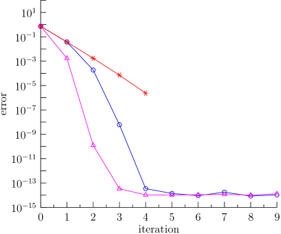
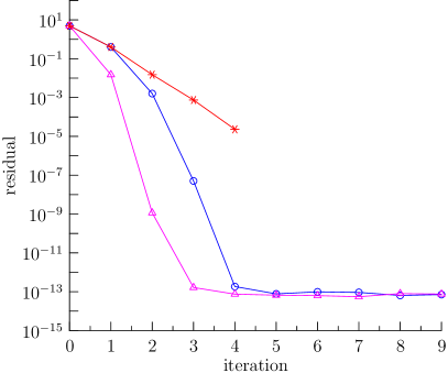
(a)	(b)

Figure 1: Convergence of (a) iterates $\|\mathbf{x}_{n}-\mathbf{x}_{*}\|$ and (b) residuals $\|f(\mathbf{x}_{n})-f(\mathbf{x}_{\text{true}})\|$, for the inverse Born series ($*$), Gauss-Newton ($\circ$) and Chebyshev-Halley ($\triangle$) methods. These methods are applied to the Neumann series problem of section 3.2.

5 Forward and inverse Born series for the Schrödinger problem
with discrete internal measurements

Recall from section 2.3 that local convergence of the forward and inverse Born series follows from showing that the forward Born operators $a_{n}$ satisfy bounds of the type (6). We show in section 5.1 that bounds of the type (6) hold for the operators $a_{n}$ for the Schrödinger problem with discrete internal measurements (defined in (33)). Then we report in section 5.2 a numerical approximation to the convergence radius of inverse Born series, in a setup related to the hydraulic tomography application of section 6.

5.1 Bounds on the forward Born operators

We recall from section 3.5 that the parameter space for this problem is $X=L^{\infty}(\widetilde{\Omega})$ where $\widetilde{\Omega}\subset\Omega$ and the distance between $\partial\Omega$ and $\partial\widetilde{\Omega}$ is positive. The difference between the unknown and the reference Schrödinger potentials is assumed to be supported in $\widetilde{\Omega}$. The measurements space is $Y=\mathbb{C}^{N\times N}$ where $N$ is the number of sources used and the norm is the entry-wise $\ell_{\infty}$ norm of a matrix in $\mathbb{C}^{N\times N}$.

The proof of lemma 2 below follows a pattern similar to [11]. There are two main differences. The first is that we work with finitely many measurements. The second is that we allow the (possibly complex) reference Schrödinger potential $q_{0}$ to be in $L^{\infty}(\Omega)$, whereas in [11] the reference potential is assumed to be constant and real. The bound (6) immediately gives a smallness condition that is sufficient for convergence of the forward Born series. The smallness condition we obtain is identical to that in [11]. This is to be expected because the underlying equation is the same and only the measurements differ.

To prove lemma 2, we need that the reference Schrödinger potential $q_{0}(\mathbf{x})\in L^{\infty}(\Omega)$ is such that the only solution to

$$\left\{\begin{aligned} -\Delta u+q_{0}u&=0,&&\text{in $\Omega$},\\ u&=0,&&\text{on $\partial\Omega$,}\end{aligned}\right.$$ (40)

is $u=0$. Such $q_{0}$ are sometimes called “non-resonant” and we assume that all the Schrödinger potentials that we deal with in what follows are non-resonant. We also need two properties for the Green function $G_{q_{0}}(\mathbf{x},\mathbf{y})$ for the Schrödinger equation (as defined in section 3.5):

1. The function $\mathbf{x}\mapsto G_{q_{0}}(\mathbf{x},\mathbf{y})$ is in $L^{1}(\Omega)$ for all $\mathbf{y}\in\Omega$.

2. The function $\mathbf{y}\mapsto\|G_{q_{0}}(\cdot,\mathbf{y})\|_{L^{1}(\Omega)}$ is in $L^{\infty}(\Omega)$.

These properties can be easily verified in both $\mathbb{R}^{2}$ and $\mathbb{R}^{3}$ for $G_{0}$ (i.e. when $q_{0}\equiv 0$) and hold for general bounded $q_{0}$. Indeed, we have $(\Delta+q_{0})(G_{q_{0}}-G_{0})=-q_{0}G_{0}$. Since the right hand side belongs to $L^{2}(\Omega)$, the difference $G_{q_{0}}-G_{0}$ must be in $H^{2}_{\text{loc}}(\Omega)$ by standard elliptic regularity estimates (see e.g. [6]) and therefore continuous (by Sobolev embeddings). This argument shows that $(G_{q_{0}}-G_{0})(\mathbf{x},\mathbf{y})$ is continuous as function of $\mathbf{x}$ and for all $\mathbf{y}$. By reciprocity $G_{q_{0}}-G_{0}$ is continuous on $\Omega\times\Omega$. Therefore $G_{q_{0}}$ satisfies the desired properties.

We can now show boundedness of the operators $a_{n}$ for the Schrödinger equation with discrete measurements. The proof of the following lemma is similar to that in [11].

Lemma 2.

Let $q_{0}(\mathbf{x})$ be a (possibly complex) non-resonant Schrödinger potential. Then the operators $a_{n}$ defined in (33) satisfy the bounds

$$||a_{n}||\leq\alpha\mu^{n},$$ (41)

with $\alpha=\nu/\mu$, and where $\nu$ and $\mu$ are constants depending on $\Omega$ and $q_{0}$ only (see equations (43) and (44) below for their definition). The norm on $a_{n}$ is the operator norm in $\mathcal{L}(X^{\otimes n},Y)$, with parameter space $X$ and data space $Y$ as in section 3.5.

Proof.

Consider $\eta_{1}\otimes\cdots\otimes\eta_{n}\in(L^{\infty}(\widetilde{\Omega}))^{\otimes n}$ and observe

$$||a_{n}(\eta_{1}\otimes\cdots\otimes\eta_{n})|| =\sup_{i,j}|(a_{n}(\eta_{1}\otimes\cdots\otimes\eta_{n}))_{i,j}|$$ (42)

$$\leq||\eta_{1}\otimes\cdots\otimes\eta_{n}||_{(L^{\infty}(\widetilde{\Omega}))^{\otimes n}}\sup_{i,j}\int_{{\widetilde{\Omega}}^{n+2}}\big{|}G_{q_{0}}(\mathbf{x},\mathbf{y}_{1})\cdot$$

$$\qquad\cdots G_{q_{0}}(\mathbf{y}_{n-1},\mathbf{y}_{n})G_{q_{0}}(\mathbf{y}_{n},\mathbf{z})\phi_{i}(\mathbf{z})\phi_{j}(\mathbf{x})\big{|}d\mathbf{z}d\mathbf{y}_{1}\cdots d\mathbf{y}_{n}d\mathbf{x}.$$

We start by estimating $||a_{1}||$ as follows,

$$||a_{1}|| \leq\sup_{i,j}\int_{{\widetilde{\Omega}}\times{\widetilde{\Omega}}\times{\widetilde{\Omega}}}{\big{|}G_{q_{0}}(\mathbf{x},\mathbf{y}_{1})G_{q_{0}}(\mathbf{y}_{1},\mathbf{z})\phi_{i}(\mathbf{z})\phi_{j}(\mathbf{x})\big{|}d\mathbf{z}d\mathbf{y}_{1}d\mathbf{x}}$$

$$\leq\sup_{i,j}\int_{\widetilde{\Omega}}\int_{\widetilde{\Omega}}\big{|}G_{q_{0}}(\mathbf{y}_{1},\mathbf{z})\phi_{i}(\mathbf{z})\big{|}d\mathbf{z}\int_{\widetilde{\Omega}}\big{|}G_{q_{0}}(\mathbf{x},\mathbf{y}_{1})\phi_{j}(\mathbf{x})\big{|}d\mathbf{x}d\mathbf{y}_{1}$$

$$\leq\sup_{i}\Bigg{(}\sup_{\mathbf{x}\in{\widetilde{\Omega}}}{\int_{\widetilde{\Omega}}\big{|}G_{q_{0}}(\mathbf{x},\mathbf{y})\phi_{i}(\mathbf{y})\big{|}d\mathbf{y}}\Bigg{)}^{2}|\Omega|.$$

Since $q_{0}$ is assumed to be non-resonant and using that $\phi_{i}\in L^{\infty}(\Omega)$, the quantity

$$\nu =\Bigg{(}\sup_{i}\sup_{\mathbf{x}\in{\widetilde{\Omega}}}{\int_{\widetilde{\Omega}}\big{|}G_{q_{0}}(\mathbf{x},\mathbf{y})\phi_{i}(\mathbf{y})\big{|}d\mathbf{y}}\Bigg{)}^{2}|\Omega|$$ (43)

is bounded. We have established that $||a_{1}||\leq\nu$.

For the remaining Born operators, we proceed recursively. Considering again (42) for $n\geq 2$, we have

$$||a_{n}|| \leq\sup_{i,j}\int_{\widetilde{\Omega}^{n+2}}\big{|}G_{q_{0}}(\mathbf{x},\mathbf{y}_{1})G_{q_{0}}(\mathbf{y}_{1},\mathbf{y}_{2})\cdot$$

$$\qquad\cdots G_{q_{0}}(\mathbf{y}_{n-1},\mathbf{y}_{n})G_{q_{0}}(\mathbf{y}_{n},\mathbf{z})\phi_{i}(\mathbf{z})\phi_{j}(\mathbf{x})\big{|}d\mathbf{z}d\mathbf{y}_{1}\cdots d\mathbf{y}_{n}d\mathbf{x}$$

$$\leq\sup_{i,j}\Bigg{(}\sup_{\mathbf{y}_{1}\in{\widetilde{\Omega}}}\int_{\widetilde{\Omega}}{\big{|}G_{q_{0}}(\mathbf{x},\mathbf{y}_{1})\phi_{j}(\mathbf{x})\big{|}d\mathbf{x}}\Bigg{)}\Bigg{(}\sup_{\mathbf{y}_{n}\in{\widetilde{\Omega}}}\int_{\widetilde{\Omega}}{\big{|}G_{q_{0}}(\mathbf{y}_{n},\mathbf{z})\phi_{i}(\mathbf{z})\big{|}d\mathbf{z}}\Bigg{)}$$

$$\cdot\int_{{\widetilde{\Omega}}^{n}}{\big{|}G_{q_{0}}(\mathbf{y}_{1},\mathbf{y}_{2})\cdots G_{q_{0}}(\mathbf{y}_{n-1},\mathbf{y}_{n})\big{|}d\mathbf{y}_{1}\cdots d\mathbf{y}_{n}}$$

$$\leq\Bigg{(}\sup_{i}\sup_{\mathbf{x}\in{\widetilde{\Omega}}}\int_{\widetilde{\Omega}}\big{|}G_{q_{0}}(\mathbf{x},\mathbf{y})\phi_{i}(\mathbf{y})\big{|}d\mathbf{y}\Bigg{)}^{2}I_{n-1}$$

where

$$I_{n-1}=\int_{{\widetilde{\Omega}}^{n}}{\big{|}G_{q_{0}}(\mathbf{y}_{1},\mathbf{y}_{2})\cdots G_{q_{0}}(\mathbf{y}_{n-1},\mathbf{y}_{n})\big{|}d\mathbf{y}_{1}\cdots d\mathbf{y}_{n}}.$$

Estimating $I_{n-1}$ we find that

$$I_{n-1} \leq\sup_{\mathbf{y}_{n-1}\in{\widetilde{\Omega}}}\int_{\widetilde{\Omega}}{\big{|}G_{q_{0}}(\mathbf{y}_{n-1},\mathbf{y}_{n})\big{|}d\mathbf{y}_{n}}\cdot\int_{{\widetilde{\Omega}}^{n-1}}{\big{|}G_{q_{0}}(\mathbf{y}_{1},\mathbf{y}_{2})\cdots G_{q_{0}}(\mathbf{y}_{n-2},\mathbf{y}_{n-1})\big{|}d\mathbf{y}_{1}\cdots d\mathbf{y}_{n-1}}$$

$$\leq\mu I_{n-2},$$

where the quantity

$$\mu=\sup_{\mathbf{x}\in{\widetilde{\Omega}}}||G_{q_{0}}(\mathbf{x},\cdot)||_{L^{1}({\widetilde{\Omega}})}$$ (44)

is finite by the properties that $G_{q_{0}}$ satisfies. Finally, noting that

$$I_{1} =\int_{{\widetilde{\Omega}}\times{\widetilde{\Omega}}}{\big{|}G_{q_{0}}(\mathbf{y}_{1},\mathbf{y}_{2})\big{|}d\mathbf{y}_{1}d\mathbf{y}_{2}}$$

$$\leq\mu|\Omega|,$$

it follows that

$$I_{n-1}\leq|\Omega|\mu^{n-1},$$

and thus

$$||a_{n}||\leq\left(\sup_{i}\sup_{\mathbf{x}\in{\widetilde{\Omega}}}||G_{q_{0}}(\mathbf{x},\cdot)||_{L^{1}(B_{\rho}(\mathbf{x}_{i}))}\right)^{2}|\Omega|\mu^{n-1}=\alpha\mu^{n}.$$

∎

Remark 2 ($L^{p}$ Bounds).

Bounds similar to those in lemma 2 can be proven when the parameter space is $X=L^{2}(\Omega)$ and the data space is $Y=\mathbb{C}^{N\times N}$, endowed with the Frobenius norm. Once we have bounds for the $\infty$ and $2$ norms, it is possible to invoke the Riesz-Thorin theorem (as in [11]) to show bounds for $2\leq p\leq\infty$ by interpolation. In this case the data space is $X=L^{p}(\Omega)$ and the parameter space is $Y=\mathbb{C}^{N\times N}$, endowed with the entry-wise $p-$norm (i.e. the $p-$norm of the $\mathbb{C}^{N^{2}}$ vector obtained by stacking the columns of a matrix in $\mathbb{C}^{N\times N}$).

Having established norm bounds on the operators $a_{n}$ for the discrete measurements Schrödinger problem, we can apply the results from section 2.3 to establish local convergence of the forward Born series, local convergence of the inverse Born series (provided the linear operator $b_{1}$ used to prime the series has sufficiently small norm, see theorem 1), stability of the inverse Born series (theorem 2) and even an error estimate (theorem 3). The actual choice of $b_{1}$ is discussed in section 7.

5.2 Numerical illustration

Applying theorem 1 to the Schrödinger problem with discrete measurements, we can expect the inverse Born series to converge when the difference $d$ between the data for the unknown and reference Schrödinger potentials satisfies

$$\|d\|\leq\frac{1}{(1+\alpha)\mu\|b_{1}\|},$$

where the constants $\alpha=\nu/\mu$ and $\mu$ are constants defined by (43) and (44) and the norms are as in section 3.5.

In preparation for the application to hydraulic tomography, we consider the setup depicted in figure 2 with computational domain $\Omega=[0,1]^{2}$. The distance between $\Omega$ and $\widetilde{\Omega}$ is $\epsilon\in[0,1/4]$ and the sources $\phi_{i}$ are supported in disks of radius $0.05$ with centers $(0.2k,0.2l)$, for $k,l=1,\ldots,4$. The sources are $\phi_{i}(\mathbf{x})=\phi(\mathbf{x}-\mathbf{x}_{i})$ where $\mathbf{x}_{i}$ is the center of the disk support and $\phi$ is an infinitely smooth function with $0\leq\phi(\mathbf{x})\leq 1$. Although theorem 1 allows for the supports of the sources to overlap, we take them to be disjoint as this is the case in the hydraulic tomography application.

The constants $\mu$ and $\nu$ are approximated by solving appropriate (forward) Schrödinger problems with $q_{0}=0$. The grid we use for this purpose is uniform and consists of the nodes $(kh,lh)$ for $k,l=0,\ldots,400$ and $h=1/400$. We display in figure 3 the radius of convergence of the inverse Born series predicted by theorem 1, assuming $\|b_{1}\|=1$. We observe that the radius of convergence increases as $\epsilon$ increases, or in other words, the larger the region where we assume the Schrödinger potential is known, the larger the perturbations in the data the method can handle.

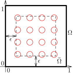
Figure 2: Setup for the numerical experiments with the Schrödinger problem with internal measurements. The domain $\Omega$ is the unit square. The domain $\widetilde{\Omega}$ where the Schrödinger potential is unknown is in dotted line and its boundary $\partial\widetilde{\Omega}$ is at a distance $\epsilon$ from $\partial\Omega$. The supports of the functions used as source terms/measurements are the red circle.

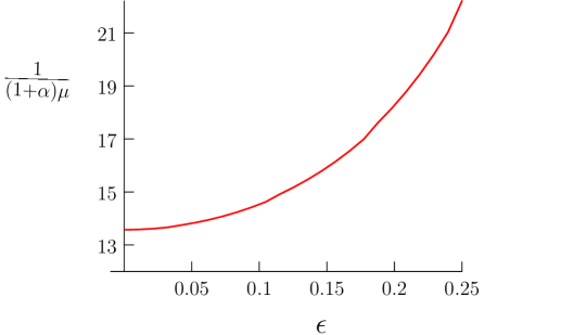
Figure 3: Numerical approximation of the radius of convergence for the inverse Born series for the Schrödinger problem with discrete internal measurements and assuming $\|b_{1}\|\geq 1$. The reference Schrödinger potential is $q_{0}=0$ and the setup is that given in figure 2.

6 Application to transient hydraulic tomography

Consider an underground aquifer confined in a bounded domain $\Omega$. The head or hydraulic pressure $u_{i}(\mathbf{x},t)$ in the aquifer due to injecting water in the $i-$th well satisfies the equation

$$\left\{\begin{aligned} S\frac{\partial u_{i}}{\partial t}&=\nabla\cdot(\sigma\nabla u_{i})-\phi_{i},&&\text{ for }\mathbf{x}\in\Omega,~{}t>0,\\ u_{i}(\mathbf{x},t)&=0,&&\text{ for }\mathbf{x}\in\partial\Omega,~{}t>0,\\ u_{i}(\mathbf{x},0)&=g(\mathbf{x}),&&\text{ for }\mathbf{x}\in\Omega.\end{aligned}\right.$$ (45)

where $i=1,\ldots,N$. Here we assume there are no sources or leaks of water in the aquifer, other than those prescribed at the wells. Hence the source term $\phi_{i}(\mathbf{x},t)$ is supported at the $i-$th well and represents the water injected at the $i-$th well. The physical properties of the aquifer are modeled by the storage coefficient $S(\mathbf{x})$ and the hydraulic conductivity $\sigma(\mathbf{x})$. The initial head (at $t=0$) is given by $g(\mathbf{x})$.

The inverse problem of hydraulic tomography that we consider here, is to determine the coefficients $\sigma$ and $S$ from knowledge of the discrete internal measurements

$$M_{i,j}(t)=\int_{\Omega}\phi_{j}(\mathbf{x},t)*u_{i}(\mathbf{x},t)d\mathbf{x},~{}i,j=1,\ldots,N,$$ (46)

where the convolution is in time. Physically these measurements correspond to time domain measurements at the $j-$th well of a spatial average of the hydraulic pressure $u_{i}$ generated by injecting in the $i-$th well. Here for simplicity, we use for the impulse response (in time) of the $j-$th measurement well the function $\phi_{j}(\mathbf{x},t)$. In a more general setup, the injection and measurement “well functions” can be different.

6.1 Reformulation as a discrete internal measurements Schrödinger problem

The frequency domain version of problem (45) is

$$\left\{\begin{aligned} \nabla\cdot(\sigma\nabla\widehat{u}_{i})-\imath\omega S\widehat{u}_{i}&=\widehat{\phi}_{i},&&\text{ for }\mathbf{x}\in\Omega,\\ \widehat{u}_{i}&=0,&&\text{ for }\mathbf{x}\in\partial\Omega,\end{aligned}\right.$$ (47)

where the hat denotes Fourier transform in time, i.e.

$$\widehat{u}_{i}(\mathbf{x},\omega)=\int_{\mathbb{R}}u_{i}(\mathbf{x},t)e^{-\imath\omega t}dt\quad\text{ and }\quad\widehat{\phi}_{i}(\mathbf{x},\omega)=\int_{\mathbb{R}}\phi_{i}(\mathbf{x},t)e^{-\imath\omega t}dt.$$

The inverse problem is now to recover $\sigma$ and $S$ from the discrete internal measurements

$$\widehat{M}_{i,j}(\omega)=\int_{\Omega}\widehat{\phi}_{j}(\mathbf{x},\omega)\widehat{u}_{i}(\mathbf{x},\omega)d\mathbf{x},$$ (48)

which is the Fourier transform in time of the discrete internal measurements for the time domain problem (46).

Next we use the Liouville transformation by defining $v_{i}=\sigma^{1/2}\widehat{u}_{i}$. If $\widehat{u}_{i}$ satisfies (47) then $v_{i}$ must satisfy the Schrödinger equation

$$\left\{\begin{aligned} \Delta v_{i}-\left(\frac{\Delta\sigma^{1/2}}{\sigma^{1/2}}+\frac{\imath\omega S}{\sigma}\right)v_{i}&=\frac{\widehat{\phi}_{i}}{\sigma^{1/2}},&&\text{ for }\mathbf{x}\in\Omega,\\ v_{i}&=0,&&\text{ for }\mathbf{x}\in\partial\Omega.\end{aligned}\right.$$ (49)

The internal measurements $\widehat{M}_{i,j}(\omega)$ can now be expressed in terms of $v_{i}$ as

$$\widehat{M}_{i,j}(\omega)=\int_{\Omega}\widehat{\phi}_{j}(\mathbf{x},\omega)\widehat{u}_{i}(\mathbf{x},\omega)d\mathbf{x}=\int_{\Omega}\frac{\widehat{\phi}_{j}(\mathbf{x},\omega)}{\sigma^{1/2}(\mathbf{x})}v_{i}(\mathbf{x},\omega)d\mathbf{x}.$$

Hence the measurements $\widehat{M}_{i,j}(\omega)$ are of the form defined in (2) with test functions $\widehat{\phi}_{i}/\sigma^{1/2}$ (modeling both injection and measurement).

If we do have access to the inside of the wells (i.e. $\mathrm{supp}\text{ }\widehat{\phi}_{i}$), it is reasonable to assume that $\sigma$ is known in $\mathrm{supp}\text{ }\widehat{\phi}_{i}$. Hence the test functions $\widehat{\phi}_{i}/\sigma^{1/2}$ are known and we can use any method for solving the inverse Schrödinger problem with discrete data to obtain an approximation to the complex Schrödinger potential

$$Q(\mathbf{x};\omega)=\frac{\Delta\sigma^{1/2}}{\sigma^{1/2}}+\frac{\imath\omega S}{\sigma},~{}\text{for $\mathbf{x}\in\Omega$}.$$ (50)

Remark 3.

A limitation of transforming the hydraulic tomography problem into an inverse Schrödinger problem is that the conductivity $\sigma$ appears as $\Delta\sigma^{1/2}/\sigma^{1/2}$ in the Schrödinger potential. Therefore any high (spatial) frequency components in $\sigma^{1/2}$ are magnified. The resulting Schrödinger potential can easily fall outside of the radius of convergence of the inverse Born series. It may be possible to overcome this limitation if we apply the inverse Born series to the hydraulic tomography problem directly (i.e. without doing the Liouville transform).

6.2 Recovery of $S$ and $\sigma$ from one frequency

Once we have approximated $Q(\mathbf{x};\omega)$ for a single (known) frequency $\omega$, the real part of $Q(\mathbf{x};\omega)$ can be used to estimate the hydraulic conductivity $\sigma$. This can be achieved by solving for $\sigma^{1/2}(\mathbf{x})$ in the equation

$$\Delta\sigma^{1/2}-\text{Re}(Q(\mathbf{x};\omega))\sigma^{1/2}=0,$$

on the aquifer without the wells, i.e.

$$\Omega^{\prime}\equiv\Omega\backslash\bigcup_{i=1}^{n}\mathrm{supp}\text{ }\widehat{\phi}_{i},$$

and with Dirichlet boundary conditions at $\partial\Omega^{\prime}$ determined from the (assumed) knowledge of $\sigma$ at the measurement wells and at $\partial\Omega$. An estimate of the storage coefficient $S$ from $\text{Im}(Q(\mathbf{x};\omega))$ and $\sigma(\mathbf{x})$ follows since

$$S(\mathbf{x})=\sigma(\mathbf{x})\text{Im}(Q(\mathbf{x};\omega))/\omega.$$

In principle, measurements $\widehat{M}_{i,j}(\omega)$ for one single frequency are enough to find both parameters $\sigma(\mathbf{x})$ and $S(\mathbf{x})$. Unfortunately, this procedure seems to be much more sensitive to changes in $\sigma$ than to changes in $S$. This is due to $\Delta\sigma^{1/2}$ appearing in the expression of $Q(\mathbf{x};\omega)$ (see remark 3). We deal with this problem by using data for two frequencies as is explained below.

6.3 Recovery of $S$ and $\sigma$ from two frequencies

Here the data we have is $\widehat{M}_{i,j}(\omega_{1})$ and $\widehat{M}_{i,j}(\omega_{2})$ for two frequencies $\omega_{1}\neq\omega_{2}$ and we use it to solve two discrete measurements Schrödinger problems for $Q(\mathbf{x};\omega_{1})$ and $Q(\mathbf{x};\omega_{2})$, for $\mathbf{x}\in\Omega$. A good rule of thumb is to choose the frequencies so that $\omega_{1}$ is sufficiently low to make $\text{Re}(Q(\mathbf{x};\omega_{1}))$ the largest term in $Q(\mathbf{x};\omega_{1})$ and $\omega_{2}$ is sufficiently large to make $\text{Im}(Q(\mathbf{x};\omega_{2}))$ the largest term in $Q(\mathbf{x};\omega_{2})$. For each point $\mathbf{x}$ in $\Omega^{\prime}$ (the domain without the wells), we solve for $r_{1}(\mathbf{x})$ and $r_{2}(\mathbf{x})$ in the $2\times 2$ system:

$$\begin{bmatrix}1&\imath\omega_{1}\\ 1&\imath\omega_{2}\end{bmatrix}\begin{bmatrix}r_{1}(\mathbf{x})\\ r_{2}(\mathbf{x})\end{bmatrix}=\begin{bmatrix}Q(\mathbf{x};\omega_{1})\\ Q(\mathbf{x};\omega_{2})\end{bmatrix}.$$ (51)

Then to estimate the conductivity we solve for $\sigma^{1/2}$ in the equation:

$$\Delta\sigma^{1/2}-r_{1}(\mathbf{x})\sigma^{1/2}=0,~{}\text{for $\mathbf{x}\in\Omega^{\prime}$},$$ (52)

with Dirichlet boundary condition given by the knowledge of $\sigma$ on $\partial\Omega^{\prime}$. Once we know $\sigma$, the storage coefficient $S$ can be easily obtained from $r_{2}$, indeed:

$$S(\mathbf{x})=\sigma(\mathbf{x})r_{2}(\mathbf{x}).$$ (53)

7 Numerical Experiments

We now present numerical experiments comparing inverse Born series with the Gauss-Newton and Chebyshev-Halley methods for both the discrete internal measurements Schrödinger problem (section 7.1) and an application to transient hydraulic tomography (section 7.2).

7.1 Schrödinger potential reconstructions from discrete internal measurements

As discussed in section 3.5, our objective is to recover an unknown Schrödinger potential $q$ from the measurements $f(q)=\mathbf{D}$, where the entries $D_{i,j}$ of the $N\times N$ matrix $\mathbf{D}$ are given by (2).

We discretize the computational domain $\Omega=[0,1]^{2}$ with a uniform grid consisting of the nodes $(kh,lh)$, for $k,l=0,\ldots,400$ and $h=1/400$. We use a total of $16$ measurement functions $\phi_{j}$, which are smooth and satisfy: $\|\phi_{j}\|_{L^{\infty}(\Omega)}=1$ for $j=1,\ldots,16$; $\phi_{j}$ is compactly supported on a circle of radius $\rho=0.05$; and the centers of the wells are uniformly spaced in the domain at the points $(0.2m,0.2n)$ for $m,n=1,\ldots,4$. The Laplacian in the Schrödinger equation is discretized with the usual five point finite differences stencil and the true Schrödinger potential is simply evaluated at the grid nodes. The measurements $D_{i,j}=\langle\phi_{j},u_{i}\rangle_{L^{2}(\Omega)}$ involve integrals that are approximated by the trapezoidal rule on the grid. Measurements $f(q_{0})$ for the reference potential $q_{0}$ are computed in the same grid. The data that we use for the reconstructions is $f(q)-f(q_{0})$.

The reconstructions are performed on a different (coarser) grid consisting of the nodes $(kh_{c},lh_{c})$ for $k,l=0,\ldots,80$ and $h_{c}=1/80$. We compare the results obtained from a truncated inverse Born series of order 5, and 10 iterations of the Gauss-Newton and Chebyshev-Halley methods. These three reconstructions are applied to $F$, a coarse grid version of the map $f$. For instance, the reconstructions for the inverse Born series are

$$\sum_{n=1}^{k}B_{n}((f(q)-f(q_{0}))^{\otimes n}),$$

where the coefficients $B_{n}$ are the inverse Born series coefficients for the coarse grid $F$ (rather than those for the fine grid $f$, which would be an inverse crime). For the inverse Born series, the operator $B_{1}$ is a regularized pseudoinverse of $A_{1}$ (i.e. the linearization of the coarse grid forward map $F$) where the singular values of $A_{1}$ which are less than $0.01$ times the largest singular value (of $A_{1}$) are treated as zero. The same regularization is used for the Jacobians involved in the Gauss-Newton and Chebyshev-Halley methods. We use $q_{0}=0$ as the reference potential for the inverse Born series as well as the initial guess for the iterative Gauss-Newton and Chebyshev-Halley methods.

Figure 4 shows the reconstructions of a real smooth Schrödinger potential $-14\leq q(\mathbf{x})\leq 4$ and a real piecewise constant potential with $-6\leq q(\mathbf{x})\leq 12$. In both cases, the potential and the generated data are small enough to satisfy the hypotheses of theorem 3. Figure 5 displays the reconstructions of the same potentials from noisy data. The noisy data is obtained by first generating the true data $f(q)-f(q_{0})$ as above, and then perturbing it with $1\%$ zero mean additive Gaussian noise, i.e. with standard deviation $0.01\max_{i,j}|(f(q)-f(q_{0}))_{i,j}|$. Similarly, figure 6 displays the reconstructions with 5% additive Gaussian noise, i.e. with zero mean and standard deviation $0.05\max_{i,j}|(f(q)-f(q_{0}))_{i,j}|$. In the experiments with noise present, the pseudoinverses of the Jacobians have been additionally regularized to compensate for the noise level (i.e. only singular values above $0.02$ (resp. $0.06$) times the largest singular value are retained for inversion for 1% (resp. 5%) noise).

Figure 4: Comparison of reconstructions of a smooth (top) and piecewise constant (bottom) Schrödinger potential from discrete internal data at 16 locations and with no noise. The color scale is identical for all images in a row.

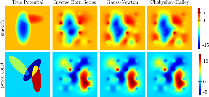
Figure 5: Comparison of reconstructions of a smooth (top) and piecewise constant (bottom) Schrödinger potential from discrete internal data at 16 locations and with 1% additive Gaussian noise. The color scale is identical for all images in a row.

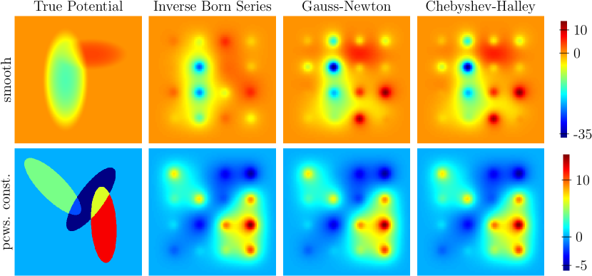
Figure 6: Comparison of reconstructions of a smooth (top) and piecewise constant (bottom) Schrödinger potential from discrete internal data at 16 locations and with 5% additive Gaussian noise. The color scale is identical for all images in a row.

7.2 Transient hydraulic tomography

In the frequency domain hydraulic tomography problem (see section 6), the objective is to estimate the hydraulic conductivity $\sigma(\mathbf{x})$ and the storage coefficient $S(\mathbf{x})$ from the frequency dependent measurements $\widehat{M}_{i,j}(\omega)$ defined in (48).

As before, the computational domain $\Omega=[0,1]^{2}$ is discretized with a uniform grid with nodes $(kh,lh)$ for $k,l=0,\ldots 400$ and $h=1/400$. The true storage coefficient $S$ is evaluated on this grid. The discretization of the term $\nabla\cdot[\sigma\nabla u]$ is done through the stencil

$$(\nabla\cdot[\sigma\nabla u])(kh,lh)\approx \sigma_{k+1/2,l}\frac{u_{k+1,l}-u_{k,l}}{h^{2}}+\sigma_{k-1/2,l}\frac{u_{k-1,l}-u_{k,l}}{h^{2}}$$

$$+ \sigma_{k,l+1/2}\frac{u_{k,l+1}-u_{k,l}}{h^{2}}+\sigma_{k,l-1/2}\frac{u_{k,l-1}-u_{k,l}}{h^{2}},$$

where $u_{k,l}\approx u(kh,lh)$ and similarly for $\sigma$. This means that the true conductivity is evaluated at the midpoints of the horizontal and vertical edges of the grid. The boundary points have a different stencil that takes into account the homogeneous Dirichlet boundary conditions, and that we do not include here for the sake of clarity.

The frequency domain measurement functions $\widehat{\phi}_{i}(\mathbf{x},\omega)$ we use are, for simplicity, independent of the frequency $\omega$ and are given in $\mathbf{x}$ by the same 16 compactly supported smooth functions described in section 7.1. The measurements $\widehat{M}_{i,j}(\omega)=\langle\widehat{\phi}_{j},\widehat{u}_{i}\rangle_{L^{2}(\Omega)}$ involve integrals over $\Omega$ that are evaluated by using the trapezoidal rule on the same grid that is used for the forward simulations. Recalling section 6.1, the measurements $\widehat{M}_{i,j}(\omega)$ can also be viewed as discrete internal measurements of a Schrödinger field $v_{i}$ (see (49)) associated with the potential $Q(\mathbf{x};\omega)$ defined in (50) i.e. ${\bf\widehat{M}(\omega)}=f(Q(\mathbf{x};\omega))$ with well functions $\widehat{\phi}_{i}/\sigma^{1/2}$. We also compute measurements for the reference potential $Q_{0}=0$ on this grid using the well functions $\widehat{\phi}_{i}/\sigma^{1/2}$ (this corresponds to $S=0$ and $\sigma=1$). The measurements we use for reconstructions are $f(Q(\mathbf{x};\omega))-f(Q_{0})$ (for two different frequencies).

Reconstructions are again performed on the coarse grid consisting of the nodes $(kh_{c},lh_{c})$ for $k,l=0,\ldots,80$ and $h_{c}=1/80$. For each method (inverse Born series order 5, Gauss-Newton, and Chebyshev-Halley), an approximation of the complex Schrödinger potential $Q(\mathbf{x};\omega)$ is found from the frequency domain data $f(Q(\mathbf{x};\omega))-f(Q_{0})$ for $\omega=1,10$. The parameters $S$ and $\sigma$ are then estimated with the procedure of section 6.3. The grid used for solving the problems (52) for the conductivity is the same coarse grid used for the reconstructions (to avoid an inverse crime). The boundary conditions for (52) are obtained from the true conductivity evaluated at appropriate points.

Figure 7 shows the reconstructions of the hydraulic conductivity $\sigma$ and storage coefficient $S$ when data has no noise. The conductivity $\sigma$ is smooth and $|1-\sigma|<0.8$. The storage coefficient $S$ is also smooth and $-5\leq S\leq 3$. We use the true conductivity $\sigma$ inside the wells but the storage coefficient $S$ inside the wells is computed, as in the rest of the domain, from (53). Reconstructions with 1% additive zero mean Gaussian noise are included in figure 8. As before this means the noise has standard deviation $0.01\max_{i,j}|[f(Q(\mathbf{x};\omega))-f(Q_{0})]_{i,j}|$, which is different for the two frequencies we use. Similarly, figure 9 displays reconstructions with 5% additive zero mean Gaussian noise.

Remark 4.

In our experiments, the parameters $\sigma$ and $S$ are chosen so that the corresponding Schrödinger potential $Q(\mathbf{x};\omega)$ and the generated data are small enough to satisfy the hypotheses of theorem 3 (for $\omega=1,10$). This makes the contrasts in $\sigma$ (especially) and $S$ too small to represent a realistic problem (see e.g. [4]). As noted before in remark 3, it may be possible to overcome this by using the inverse Born series on the hydraulic tomography problem directly.

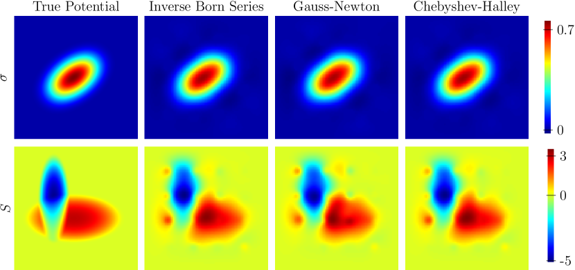
Figure 7: Hydraulic tomography reconstructions of the hydraulic conductivity $\sigma(\mathbf{x})$ (top) and the storage coefficient $S(\mathbf{x})$ (bottom) for noiseless data and different methods.

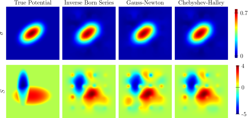
Figure 8: Hydraulic tomography reconstructions of the hydraulic conductivity $\sigma(\mathbf{x})$ (top) and the storage coefficient $S(\mathbf{x})$ (bottom) for data with 1% additive Gaussian noise and different methods.

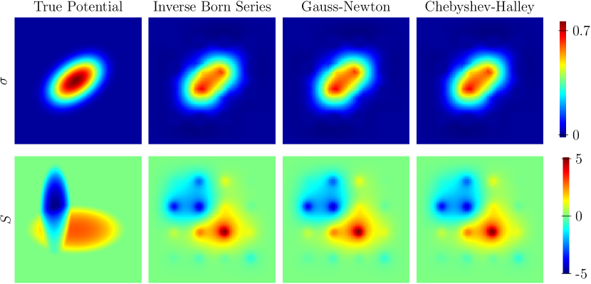
Figure 9: Hydraulic tomography reconstructions of the hydraulic conductivity $\sigma(\mathbf{x})$ (top) and the storage coefficient $S(\mathbf{x})$ (bottom) for data with 5% additive Gaussian noise and different methods.

8 Discussion

We show here that with little modification, the inverse Born series convergence results of Moskow and Schotland [11] can be generalized to mappings between Banach spaces. With this abstraction, we only need to show that the forward Born operators are bounded as in (6) to obtain convergence, stability and error estimates for the inverse Born series. Such results are then proven for the problem of finding the Schrödinger potential from discrete internal measurements. A nice byproduct of our approach is that we can relate forward and inverse Born series coefficients (up to a symmetrization) to the Taylor series coefficients of an analytic map and its inverse (provided it exists).

Since the cost of computing the $n-$th term of the inverse Born series increases exponentially in $n$, we also consider the iterative method obtained by restarting the inverse Born series after summing the first $k$ terms. We obtain a class of methods that we call RIBS($k$) and that includes the well-known Gauss-Newton and Chebyshev-Halley iterative methods. Our numerical results show these methods give reconstructions comparable to those obtained with the inverse Born series.

Among the future directions of this work would be to show the RIBS($k$) method is convergent. We conjecture that the convergence rate of RIBS($k$) is of order $k$. The RIBS($k$) method is only locally convergent, meaning that we need to be already close to the solution for the method to converge. Globalization strategies that keep, when possible, this higher order convergence rate are needed.

The application we use to illustrate our method is a problem related to transient hydraulic tomography. Since we convert this problem to the problem of finding a Schrödinger potential and all the methods we use here are locally convergent, the contrasts that we can deal with are far from realistic ones. We believe that a proper globalization strategy will allow us to deal with higher contrasts. Another important question that we have not dealt with here is that of regularization. The only regularization that we consider here is the choice of the linear operator that primes the inverse Born series. By analogy with what can be done with the Gauss-Newton method, we believe it is possible to include specific a priori information about the true parameters by formulating the problem as minimizing the misfit plus a penalty term that takes into account the a priori information.

Appendix A Inverse Born series in Banach spaces

The proofs in this appendix are an adaptation of the proofs in Moskow and Schotland [11] to inverse Born series in Banach spaces. The results are stated in section 2.3.

A.1 Proof of bounds for inverse Born series coefficients (lemma 1)

Proof.

Since $\|a_{n}\|\leq\alpha\mu^{n}$, we can estimate for $n\geq 2$:

$$\|b_{n}\| \leq\sum_{m=1}^{n-1}\sum_{s_{1}+\cdots+s_{m}=n}\|b_{m}\|\|a_{s_{1}}\|\cdots\|a_{s_{m}}\|\|b_{1}\|^{n}$$ (54)

$$\leq\|b_{1}\|^{n}\sum_{m=1}^{n-1}\|b_{m}\|\sum_{s_{1}+\cdots+s_{m}=n}(\alpha\mu^{s_{1}})\ldots(\alpha\mu^{s_{m}})$$

$$=\|b_{1}\|^{n}\mu^{n}\sum_{m=1}^{n-1}\|b_{m}\|\alpha^{m}\sum_{s_{1}+\cdots+s_{m}=n}1.$$

The last sum is the number of partitions of the integer $n$ into $m$ ordered parts. Hence for $n\geq 2$, we get

$$\|b_{n}\| \leq(\mu\|b_{1}\|)^{n}\sum_{m=1}^{n-1}\|b_{m}\|\alpha^{m}{n-1\choose m-1}$$ (55)

$$\leq(\mu\|b_{1}\|)^{n}\left(\sum_{m=1}^{n-1}\|b_{m}\|\right)\left(\sum_{m=1}^{n-1}\alpha^{m}{n-1\choose m-1}\right)$$

$$\leq(\mu\|b_{1}\|(\alpha+1))^{n}\sum_{m=1}^{n-1}\|b_{m}\|.$$

To get the last inequality we used that

$$\sum_{m=1}^{n-1}\alpha^{m}{n-1\choose m-1}=\sum_{m=0}^{n-2}\alpha^{m+1}{n-1\choose m}\leq\alpha\sum_{m=0}^{n-1}\alpha^{m+1}{n-1\choose m}=\alpha(1+\alpha)^{n-1}\leq(1+\alpha)^{n}.$$

Following [11] we can estimate the coefficients in the inverse Born series by

$$\|b_{n}\|\leq C_{n}(\mu\|b_{1}\|(\alpha+1))^{n}\|b_{1}\|,~{}\text{for}~{}n\geq 2,$$ (56)

where the constants $C_{n}$ are defined recursively by

$$C_{2}=1~{}\text{and}~{}C_{n+1}=1+((\alpha+1)\mu\|b_{1}\|)^{n}~{}\text{for $n\geq 2$.}$$ (57)

The constants $C_{n}$ are then

$$C_{n}=\prod_{m=2}^{n-1}(1+((\alpha+1)\mu\|b_{1}\|)^{m})\leq\exp\left(\frac{1}{1-(\alpha+1)\mu\|b_{1}\|}\right).$$ (58)

where the bound for $C_{n}$ can be derived as in [11] and is valid when $(\alpha+1)\mu\|b_{1}\|<1$, which is one of the hypothesis. The result follows from the bounds (56) and (58). ∎

A.2 Proof of local convergence of inverse Born series (theorem 1)

Proof.

Using the estimate of lemma 1, we can dominate the term of the inverse Born series by a geometric series as follows

$$\|b_{n}(d^{n})\| \leq\beta((\alpha+1)\mu\|b_{1}\|\|d\|)^{n}.$$ (59)

Therefore the Born series is absolutely convergent when $(\alpha+1)\mu\|b_{1}\|\|d\|<1$, which is one of the assumptions of this theorem. The tail of the series with terms the absolute values of the inverse Born series terms, can be estimated by noticing that:

$$\sum_{N+1}^{\infty}\beta((\alpha+1)\mu\|b_{1}\|\|d\|)^{n}=\beta\frac{((\alpha+1)\mu\|b_{1}\|\|d\|)^{N+1}}{1-(\alpha+1)\mu\|b_{1}\|\|d\|}.$$ (60)

∎

A.3 Proof of stability of inverse Born series (theorem 2)

Proof.

We use an identity on tensor products to conclude that

$$\|h_{1}-h_{2}\| \leq\sum_{n=1}^{\infty}\|b_{n}(d_{1}^{\otimes n}-d_{2}^{\otimes n})\|$$ (61)

$$=\sum_{n=1}^{\infty}\left\|b_{n}\left(\sum_{k=0}^{n-1}d_{1}^{\otimes k}\otimes(d_{1}-d_{2})\otimes d_{2}^{\otimes(n-k-1)}\right)\right\|$$

$$\leq\sum_{n=1}^{\infty}nM^{n-1}\|b_{n}\|\|d_{1}-d_{2}\|.$$

The desired estimate follows from applying the estimate for the $\|b_{n}\|$ in lemma 1,

$$\|h_{1}-h_{2}\| \leq\|d_{1}-d_{2}\|\sum_{n=1}^{\infty}nM^{n-1}\beta((\alpha+1)\mu\|b_{1}\|)^{n}$$ (62)

$$\leq\|d_{1}-d_{2}\|\frac{\beta}{M}\frac{1}{(1-M(\alpha+1)\mu\|b_{1}\|)^{2}},$$

since we assumed that $M(\alpha+1)\mu\|b_{1}\|<1$. Here we used the following inequality:

$$\beta\sum_{n=1}^{\infty}nM^{n-1}\delta^{n}=\frac{\beta}{M}\sum_{n=1}^{\infty}n(M\delta)^{n}\leq\frac{\beta}{M}\sum_{n=0}^{\infty}(n+1)(M\delta)^{n}=\frac{\beta}{M}\frac{1}{(1-M\delta)^{2}}$$

where $\delta\equiv(\alpha+1)\mu\|b_{1}\|$. ∎

A.4 Proof of inverse Born series error estimate (theorem 3)

Proof.

Taking the expression for $d$ in (17) and replacing in the expression for $h_{*}$ in (17) we get:

$$h_{*}=\sum_{n=1}^{\infty}c_{n}(h^{\otimes n}),$$ (63)

where

$$c_{1} =b_{1}a_{1},$$ (64)

$$c_{n} =\left(\sum_{m=1}^{n-1}b_{m}\left(\sum_{s_{1}+\cdots s_{m}=n}a_{s_{1}}\otimes\cdots\otimes a_{s_{m}}\right)\right)+b_{n}(a_{1}^{\otimes n}),~{}\text{for $n\geq 2$.}$$

Using the expression (10) of $b_{n}$ in terms of $b_{m}$, $1\leq m\leq n-1$, we get for $n\geq 2$ that

$$c_{n}=\sum_{m=1}^{n-1}b_{m}\left(\sum_{s_{1}+\cdots s_{m}=n}a_{s_{1}}\otimes\cdots\otimes a_{s_{m}}\right)\left(I-(b_{1}a_{1})^{\otimes n}\right).$$ (65)

Hence the reconstruction error is

$$h-h_{*}=(h-b_{1}a_{1}h)-\sum_{n=2}^{\infty}\sum_{m=1}^{n-1}b_{m}\left(\sum_{s_{1}+\cdots s_{m}=n}a_{s_{1}}\otimes\cdots\otimes a_{s_{m}}\right)\left(h^{\otimes n}-(b_{1}a_{1}h)^{\otimes n}\right).$$ (66)

We now estimate the error:

$$\|h-h_{*}\|\leq\|h-b_{1}a_{1}h\|+\sum_{n=2}^{\infty}\sum_{m=1}^{n-1}\sum_{s_{1}+\cdots s_{m}=n}\|b_{m}\|\|a_{s_{1}}\|\cdots\|a_{s_{m}}\|\left\|h^{\otimes n}-(b_{1}a_{1}h)^{\otimes n}\right\|.$$ (67)

For $n\geq 1$ we can estimate:

$$\|h^{\otimes n}-(b_{1}a_{1}h)^{\otimes n}\| =\left\|\sum_{k=0}^{n-1}h^{\otimes k}\otimes(h-b_{1}a_{1}h)\otimes(b_{1}a_{1}h)^{\otimes(n-k-1)}\right\|$$ (68)

$$\leq nM^{n-1}\|h-b_{1}a_{1}h\|,$$

where we used the hypothesis $\|h\|\leq M$, $\|b_{1}a_{1}h\|\leq M$. Since we assumed the Born series coefficients satisfy $\|a_{n}\|\leq\alpha\mu^{n}$ we get:

$$\|h-h_{*}\| \leq\|h-b_{1}a_{1}h\|\left(1+\sum_{n=2}^{\infty}\sum_{m=1}^{n-1}\sum_{s_{1}+\cdots s_{m}=n}\|b_{m}\|(\alpha\mu^{s_{1}})\cdots(\alpha\mu^{s_{m}})nM^{n-1}\right)$$ (69)

$$=\|h-b_{1}a_{1}h\|\left(1+\sum_{n=2}^{\infty}\sum_{m=1}^{n-1}\|b_{m}\|\alpha^{m}n\mu^{n}M^{n-1}{n-1\choose m-1}\right).$$

Here we have used again the fact that the number of ordered partitions of $n$ into $m$ integers is:

$$\sum_{s_{1}+\cdots s_{m}=n}1={n-1\choose m-1}.$$

Clearly we have that:

$$\|h-h_{*}\|\leq\|h-b_{1}a_{1}h\|\left(1+\sum_{n=2}^{\infty}n\mu^{n}M^{n-1}\left(\sum_{m=1}^{n-1}\|b_{m}\|\right)\left(\sum_{m=1}^{n-1}\alpha^{m}{n-1\choose m-1}\right)\right).$$ (70)

Now using the two facts:

$$\sum_{m=1}^{n-1}\|b_{m}\| \leq\beta\sum_{m=1}^{n-1}((\alpha+1)\mu\|b_{1}\|)^{m}~{}\text{(lemma~{}\ref{lem:bj})},$$ (71)

$$\sum_{m=1}^{n-1}\alpha^{m}{n-1\choose m-1} \leq(1+\alpha)^{n}~{}\text{(as in \eqref{eq:binomial})},$$

we get the inequality

$$\|h-h_{*}\|\leq\|h-b_{1}a_{1}h\|\left(1+\sum_{n=2}^{\infty}\frac{n}{M}(\mu M(1+\alpha))^{n}\beta\sum_{m=1}^{n-1}((\alpha+1)\mu\|b_{1}\|)^{m}\right).$$ (72)

Adding the $m=0$ term to the geometric series over $m$ and summing we get:

$$\|h-h_{*}\|\leq\|h-b_{1}a_{1}h\|\left(1+\frac{\beta}{M}\sum_{n=1}^{\infty}n(\mu M(1+\alpha))^{n}\frac{1-((\alpha+1)\mu\|b_{1}\|)^{n}}{1-(\alpha+1)\mu\|b_{1}\|}\right).$$ (73)

The hypothesis $\mu M(\alpha+1)<1$ and $\mu(\alpha+1)\|b_{1}\|<1$ imply the quantitity in parenthesis is bounded and depends only on $M$, $\alpha$, $\beta$ and $\mu$ and $\|b_{1}\|$. ∎

References

- Arridge et al. [2012] S. Arridge, S. Moskow, and J. C. Schotland. Inverse Born series for the Calderon problem. Inverse Problems, 28(3):035003, 16, 2012. ISSN 0266-5611. doi: 10.1088/0266-5611/28/3/035003.
- Arridge [1999] S. R. Arridge. Optical tomography in medical imaging. Inverse Problems, 15(2):R41, 1999. doi: 10.1088/0266-5611/15/2/022.
- Borcea [2002] L. Borcea. Electrical impedance tomography. Inverse Problems, 18:R99–R136, 2002. doi: 10.1088/0266-5611/18/6/201. Topical Review.
- Cardiff and Barrash [2011] M. Cardiff and W. Barrash. 3-D transient hydraulic tomography in unconfined aquifers with fast drainage response. Water Resources Research, 47(12):W12518, 2011. ISSN 1944-7973. doi: 10.1029/2010WR010367.
- Deuflhard [2011] P. Deuflhard. Newton methods for nonlinear problems, volume 35 of Springer Series in Computational Mathematics. Springer, Heidelberg, 2011. ISBN 978-3-642-23898-7. doi: 10.1007/978-3-642-23899-4. Affine invariance and adaptive algorithms, First softcover printing of the 2006 corrected printing.
- Evans [2010] L. Evans. Partial Differential Equations, 2nd Edition. American Mathematical Society, 2010.
- Hettlich and Rundell [2000] F. Hettlich and W. Rundell. A second degree method for nonlinear inverse problems. SIAM J. Numer. Anal., 37(2):587–620 (electronic), 2000. ISSN 0036-1429. doi: 10.1137/S0036142998341246.
- Kilgore et al. [2012] K. Kilgore, S. Moskow, and J. C. Schotland. Inverse Born series for scalar waves. J. Comput. Math., 30(6):601–614, 2012. ISSN 0254-9409. doi: 10.4208/jcm.1205-m3935.
- Markel and Schotland [2007] V. A. Markel and J. C. Schotland. On the convergence of the Born series in optical tomography with diffuse light. Inverse Problems, 23(4):1445–1465, 2007. ISSN 0266-5611. doi: 10.1088/0266-5611/23/4/006.
- Markel et al. [2003] V. A. Markel, J. A. O’Sullivan, and J. C. Schotland. Inverse problem in optical diffusion tomography. iv. nonlinear inversion formulas. J. Opt. Soc. Am. A, 20(5):903–912, May 2003. doi: 10.1364/JOSAA.20.000903.
- Moskow and Schotland [2008] S. Moskow and J. C. Schotland. Convergence and stability of the inverse scattering series for diffuse waves. Inverse Problems, 24(6):065005, 16, 2008. ISSN 0266-5611. doi: 10.1088/0266-5611/24/6/065005.
- Moskow and Schotland [2009] S. Moskow and J. C. Schotland. Numerical studies of the inverse Born series for diffuse waves. Inverse Problems, 25(9):095007, 18, 2009. ISSN 0266-5611. doi: 10.1088/0266-5611/25/9/095007.
- Whittlesey [1965] E. F. Whittlesey. Analytic functions in Banach spaces. Proc. Amer. Math. Soc., 16:1077–1083, 1965. ISSN 0002-9939.
- Zeidler [1986] E. Zeidler. Nonlinear functional analysis and its applications. I. Springer-Verlag, New York, 1986. ISBN 0-387-90914-1. doi: 10.1007/978-1-4612-4838-5. Fixed-point theorems, Translated from the German by Peter R. Wadsack.