Understanding early indicators of critical transitions in power systems from autocorrelation functions

Abstract

Many dynamical systems, including power systems, recover from perturbations more slowly as they approach critical transitions—a phenomenon known as critical slowing down. If the system is stochastically forced, autocorrelation and variance in time-series data from the system often increase before the transition, potentially providing an early warning of coming danger. In some cases, these statistical patterns are sufficiently strong, and occur sufficiently far from the transition, that they can be used to predict the distance between the current operating state and the critical point. In other cases CSD comes too late to be a good indicator. In order to better understand the extent to which CSD can be used as an indicator of proximity to bifurcation in power systems, this paper derives autocorrelation functions for three small power system models, using the stochastic differential algebraic equations (SDAE) associated with each. The analytical results, along with numerical results from a larger system, show that, although CSD does occur in power systems, its signs sometimes appear only when the system is very close to transition. On the other hand, the variance in voltage magnitudes consistently shows up as a good early warning of voltage collapse. Finally, analytical results illustrate the importance of nonlinearity to the occurrence of CSD.

I Introduction

There is increasing evidence that time-series data taken from stochastically forced dynamical systems show statistical patterns that can be useful in predicting the proximity of a system to critical transitions [1], [2]. Collectively this phenomenon is known as Critical Slowing Down, and is most easily observed by testing for autocorrelation and variance in time-series data. Increases in autocorrelation and variance have been shown to give early warning of critical transitions in climate models [3], ecosystems [4], the human brain [5] and electric power systems [6, 7, 8].

Scheffer et al. [1] provide some explanation for why increasing variance and autocorrelation can indicate proximity to a critical transition. They illustrate that increasing autocorrelation results from the system returning to equilibrium more slowly after perturbations, and that increased variance results from state variables spending more time further away from equilibrium. Some further explanation of CSD in stochastic systems can be found by looking at the theory of fast-slow systems [9]. In many stochastic systems with critical transitions there are two time scales; slow trends gradually move the “equilibrium” operating state toward, or away from points of instability, and random perturbations cause fast changes in the state variables. In power systems, loads have slow predictable trends, such as load ramps in the morning hours, and fast stochastic ones, such as random load switching or rapid changes in renewable generation. Reference [9] uses the mathematical theory of the stochastic fast-slow dynamical systems and the Fokker–Planck equation to explain the use of autocorrelation and variance as indicators of CSD.

While CSD is a general property of critical transitions [10], its signs do not always appear early enough to be useful as an early warning, and do not universally appear in all variables [10, 11]. References [10] and [11] both show, using ecological models, that the signs of CSD appear only in a few of the variables, or even not at all.

Several types of critical transitions in deterministic power system models have been explained using bifurcation theory. Reference [12] explains voltage collapse as a saddle-node bifurcation. Reference [13] describes voltage instability caused by the violation of equipment limits using limit-induced bifurcation theory. Some types of oscillatory instability can be explained as a Hopf bifurcation [14], [15]. Reference [16] describes an optimization method that can find saddle-node or limit-induced bifurcation points. Reference [17] shows that both Hopf and saddle-node bifurcations can be identified in a multi-machine power system, and that their locations can be affected by a power system stabilizer. In [18], authors computed the singular points of the differential and algebraic equations that model the power system.

Substantial research has focused on estimating the proximity of a power system to a particular critical transition. References [13],[19]–[21] describe methods to measure the distance between an operating state and voltage collapse with respect to slow-moving state variables, such as load. Although these methods provide valuable information about system stability, they are based on the assumption that the current network model is accurate. However, all power system models include error, both in state variable estimates and network parameters, particularly for areas of the network that are outside of an operator’s immediate control.

An alternate approach to estimating proximity to bifurcation is to study the response of a system to stochastic forcing, such as fluctuations in load, or variable production from renewable energy sources. To this end, a growing number of papers study power system stability using stochastic models [22]–[26]. Reference [22] models power systems using Stochastic Differential Equations (SDEs) in order to develop a measure of voltage security. In [25], numerical methods are used to assess transient stability in power systems, given fluctuating loads and random faults. Reference [26] uses the Fokker-Planck equation to calculate the probability density function (PDF) for state variables in a single machine infinite bus system (SMIB), and uses the time evolution of this PDF to show how random load fluctuations affect system stability.

The results above clearly show that power system stability is affected by stochastic forcing. However, they provide little information about the extent to which CSD can be used as an early warning of critical transitions given fluctuating measurement data. Given the increasing availability of high-sample-rate synchronized phasor measurement unit (PMU) data, and the fact that insufficient situational awareness has been identified as a critical contributor to recent large power system failures (e.g., [27], [28]) there is a need to better understand how statistical phenomena, such as CSD, might be used to design good indicators of stress in power systems.

Results from the literature on CSD suggest that autocorrelation and variance in time-series data increase before critical transitions. Empirical evidence for increasing autocorrelation and variance is provided for an SMIB and a 9-bus test case in [6]. Reference [29] shows that voltage variance at the end of a distribution feeder increases as it approaches voltage collapse. However, the results do not provide insight into autocorrelation. To our knowledge, only [7, 8] derive approximate analytical autocorrelation functions (from which either autocorrelation or variance can be found) for state variables in a power system model, which is applied to the New England 39 bus test case. However, the autocorrelation function in [7, 8] is limited to the operating regime very close to the threshold of system instability. Furthermore, there is, to our knowledge, no existing research regarding which variables show the signs of CSD most clearly in power system, and thus which variables are better indicators of proximity to critical transitions. In [30], the authors derived the general autocorrelation function for the stochastic SMIB system. This paper extends the SMIB results in [30], and studies two additional power system models using the same analytical approach. Also, this paper includes new numerical simulation results for two multi-machine systems, which illustrate insights gained from the analytical work.

Motivated by the need to better understand CSD in power systems, the goal of this paper is to describe and explain changes in the autocorrelation and variance of state variables in several power system models, as they approach bifurcation. To this end, we derive autocorrelation functions of state variables for three small models. We use the results to show that CSD does occur in power systems, explain why it occurs, and describe conditions under which autocorrelation and variance signal proximity to critical transitions. The remainder of this paper is organized as follows. Section II describes the general mathematical model and the method used to derive autocorrelation functions in this paper. Analytical solutions and illustrative numerical results for three small power systems are presented in Secs. III, IV and V. In Sec. VI, the results of numerical simulations on two multi-machine power system models including the New England 39 bus test case are presented. Finally, Sec. VII summarizes the results and contributions of this paper.

II Solution Method for Autocorrelation Functions

In this section, we present the general form of the Stochastic Differential Algebraic Equations (SDAEs) used to model the three systems studied in this paper. Then, the solution of the SDAEs and the expressions for autocorrelations and variances of both algebraic and differential variables of the systems are presented. Finally, the method used for simulating the SDAEs numerically is described.

II-A The Model

All three models studied analytically in this paper include a single second-order synchronous generator. These systems can be described by the following SDAEs:

$$\ddot{\delta}+2\gamma\dot{\delta}+F_{1}\left(\delta,\underline{y},\eta\right) = 0$$ (1)

$$\underline{F_{2}}\left(\delta,\underline{y},\eta\right) = 0$$ (2)

where $\delta$ is angle of the synchronous generator’s rotor relative to a synchronously rotating reference axis, $\underline{y}$ is the vector of algebraic variables, $\gamma$ is the damping coefficient, $F_{1},\underline{F_{2}}$ form a set of nonlinear algebraic equations of the systems, and $\eta$ is a Gaussian random variable. $\eta$ has the following properties:

$$\textnormal{{E}}\left[\eta\left(t\right)\right] = 0$$ (3)

$$\textnormal{{E}}\left[\eta\left(t\right)\eta\left(s\right)\right] = \sigma_{\eta}^{2}\cdot\delta_{I}\left(t-s\right)$$ (4)

where $t,s$ are two arbitrary times, $\sigma_{\eta}^{2}$ is the intensity of noise, and $\delta_{I}$ represents the unit impulse (delta) function (which should not be confused with the rotor angle $\delta$). There are a variety of sources of noise, such as random load switching or variable renewable generation, in power systems. To our knowledge, no existing studies have quantified the correlation time of noise in power systems. Thus, in this paper, we assume that the correlation time of noise is negligible relative to the response-time of the system, which means that $\mbox{E}[\eta(t)\eta(s)]=0$ for all $s$ significantly greater than $t$. It is important to note that the variance of $\eta$ is infinite according to (4), because the delta function is infinite at $t=s$, which means that particular care is needed when simulating (1) and (2) numerically (see Sec. II-C).

In order to solve (1) and (2) analytically, we linearized $F_{1}$ and $\underline{F_{2}}$ around the stable equilibrium point using first-order Taylor expansion. Then (1) and (2) were combined into a single damped harmonic oscillator equation with stochastic forcing:

$$\Delta\ddot{\delta}+2\gamma\Delta\dot{\delta}+\omega_{0}^{2}\Delta\delta=-f\eta$$ (5)

where $\omega_{0}$ is the undamped angular frequency of the oscillator, $f$ is a constant, and $\Delta\delta=\delta-\delta_{0}$ is the deviation of the rotor angle from its equilibrium value. Both $\omega_{0}$ and $f$ change with the system’s equilibrium operating state. Equation (5) can be written as a multivariate Ornstein–Uhlenbeck process [31]:

$$\dot{\underline{z}}\left(t\right)=A\underline{z}\left(t\right)+B\left[\begin{array}[]{c}0\\ \eta\left(t\right)\end{array}\right]$$ (6)

where $\underline{z}=\left[\begin{array}[]{cc}\Delta\delta&\Delta\dot{\delta}\end{array}\right]^{T}$ is the vector of differential variables, $\Delta\dot{\delta}$ is the deviation of the generator speed from its equilibrium value, and $A$ and $B$ are constant matrices as follows:

$$A = \left[\begin{array}[]{cc}0&1\\ -\omega_{0}^{2}&-2\gamma\end{array}\right]$$ (9)

$$B = \left[\begin{array}[]{cc}0&0\\ 0&-f\end{array}\right]$$ (12)

Given (9), the eigenvalues of $A$ are $-\gamma\pm\sqrt{\gamma^{2}-\omega_{0}^{2}}$. At $\omega_{0}=0$, one of the eigenvalues of matrix $A$ becomes zero, and the system experiences a saddle-node bifurcation.

Equation (5) can be interpreted in two different ways: using either It$\hat{o}$ SDE and Stratonovich SDEs. In the It$\hat{o}$ interpretation [32], noise is considered to be uncorrelated. However, in the Stratonovich interpretation [33], which is a more natural choice physically, noise has finite, albeit very small, correlation time [31]. It$\hat{o}$ calculus is often used in discrete systems, such as finance, though a few papers have applied the It$\hat{o}$ approach to power systems [22], [25]. On the other hand, the Stratonovich method is often used in continuous physical systems or systems with band-limited noise [34]. The Stratonovich interpretation also allows the use of ordinary calculus, which is not possible with the It$\hat{o}$ interpretation. Because $B$ is a constant matrix in this paper, the It$\hat{o}$ and Stratonovich interpretations result in the same solution [34]. This paper follows the Stratonovich interpretation because it allows one to use ordinary calculus.

Following the method in [35], if $\gamma<\omega_{0}$ (which holds until very close to the bifurcation in two of our systems), the solution of (6) is as follows:

$$\Delta\delta(t) = f\cdot\int_{-\infty}^{t}\exp\left(\gamma\left(t^{\prime}-t\right)\right)\eta\left(t^{\prime}\right)\cdot$$

$$\qquad\frac{\sin\left(\omega^{\prime}(t^{\prime}-t)\right)}{\omega^{\prime}}dt^{\prime}$$

$$\Delta\dot{\delta}\left(t\right) =- f\cdot\int_{-\infty}^{t}\exp\left(\gamma\left(t^{\prime}-t\right)\right)\eta\left(t^{\prime}\right)\cdot$$

$$\qquad\frac{\sin\left(\omega^{\prime}(t^{\prime}-t)+\phi\right)\omega_{0}}{\omega^{\prime}}dt^{\prime}$$

where $t^{\prime}$ is the variable of integration, $\omega^{\prime}=\sqrt{\omega_{0}^{2}-\gamma^{2}}$ is the frequency of the underdamped harmonic oscillator, and $\phi=\arctan(\omega^{\prime}/\gamma)$.

In the system considered in Sec. IV, $\omega_{0}$ in (5) is equal to zero for all system parameters, so the condition $\gamma<\omega_{0}$ does not hold. Therefore, the solution of (5) in that system is different from (II-A), (II-A) as follows:

$$\Delta\dot{\delta}=-f\int_{-\infty}^{t}\exp\left(-2\gamma\left(t-t^{\prime}\right)\right)\eta\left(t^{\prime}\right)dt^{\prime}$$ (15)

II-B Autocorrelation and Variance of Differential Variables

Given that the eigenvalues of $A$ have negative real part before the bifurcation (because $\gamma>0$), one can calculate the stationary variances and autocorrelations of $\Delta\delta$ and $\Delta\dot{\delta}$ using (3), (4), (II-A) and (II-A). The variances of the differential variables are as follows:

$$\sigma_{\Delta\delta}^{2} = \frac{f^{2}\sigma_{\eta}^{2}}{4\gamma\omega_{0}^{2}}$$ (16)

$$\sigma_{\Delta\dot{\delta}}^{2} = \frac{f^{2}\sigma_{\eta}^{2}}{4\gamma}$$ (17)

If $\gamma<\omega_{0}$, the normalized autocorrelation functions for $\Delta\delta$ and $\Delta\dot{\delta}$ are as follows:

$$\frac{\text{E}\left[\Delta\delta\left(t\right)\Delta\delta\left(s\right)\right]}{\sigma_{\Delta\delta}^{2}} = \exp\left(-\gamma\Delta t\right)\frac{\omega_{0}}{\omega^{\prime}}\cdot$$

$$\sin\left(\omega^{\prime}\Delta t+\phi\right)$$

$$\frac{\text{E}\left[\Delta\dot{\delta}\left(t\right)\Delta\dot{\delta}\left(s\right)\right]}{\sigma_{\Delta\dot{\delta}}^{2}} = \exp\left(-\gamma\Delta t\right)\frac{-\omega_{0}}{\omega^{\prime}}\cdot$$

$$\sin\left(\omega^{\prime}\Delta t-\phi\right)$$

where $\Delta t=t-s$.

If $\omega_{0}=0$, the variance of $\Delta\dot{\delta}$ can be calculated from (17) and the autocorrelation of $\Delta\dot{\delta}$ is as follows:

$$\frac{\text{E}\left[\Delta\dot{\delta}\left(t\right)\Delta\dot{\delta}\left(s\right)\right]}{\sigma_{\Delta\dot{\delta}}^{2}}=\exp\left(-2\gamma\Delta t\right)$$ (20)

II-C Autocorrelation and Variance of Algebraic Variables

In order to compute the autocorrelation functions of the algebraic variables, we calculated the algebraic variables as linear functions of the differential variable $\Delta\delta$ and the noise $\eta$, by linearizing $\underline{F_{2}}$ in (2):

$$\Delta y_{i}\left(t\right)=C_{i_{,}1}\Delta\delta\left(t\right)+C_{i_{,}2}\eta$$ (21)

where $y_{i}$ is an algebraic variable, and $C_{i_{,}1},C_{i_{,}2}$ are constant values. Then, the autocorrelation of $\Delta y_{i}$ is as follows for $t\geq s$:

$$\text{E}\left[\Delta y_{i}\left(t\right)\Delta y_{i}\left(s\right)\right] = C_{i_{,}1}^{2}\cdot\text{E}\left[\Delta\delta\left(t\right)\Delta\delta\left(s\right)\right]+$$

$$C_{i_{,}1}C_{i_{,}2}\mbox{$\cdot$}\textnormal{E}\left[\Delta\delta\left(t\right)\eta\left(s\right)\right]+$$

$$C_{i_{,}2}^{2}\cdot\text{E}\left[\eta\left(t\right)\eta\left(s\right)\right]$$

In deriving (II-C), we used the fact that $\textnormal{{E}}\left[\Delta\delta\left(s\right)\eta\left(t\right)\right]=0$ since the system is causal. Equation (II-C) shows that, in order to calculate the autocorrelation of $\Delta y_{i}\left(t\right)$, it is necessary to calculate $\textnormal{{E}}\left[\Delta\delta\left(t\right)\eta\left(s\right)\right]$. Using (II-A), $\textnormal{{E}}\left[\Delta\delta\left(t\right)\eta\left(s\right)\right]$ is as follows:

$$\textnormal{{E}}\left[\Delta\delta\left(t\right)\eta\left(s\right)\right] = -\exp\left(-\gamma\Delta t\right)\cdot\frac{f}{\omega^{\prime}}\cdot$$

$$\sin\left(\omega^{\prime}\Delta t\right)\sigma_{\eta}^{2}$$

which indicates that $\textrm{cov}\left(\Delta\delta,\eta\right)=0$.

In order to use (II-C) to compute the variance of $\Delta y_{i}$, we need to carefully consider our model of noise in numerical computations. According to (4), the variance of $\eta$ is infinite, because the delta function is infinite at $t=s$, which would mean that the variance of $\Delta y_{i}$ could be infinite. However, the noise in numerical simulations must have a finite variance. To determine it, we rewrite (6) as follows:

$$d\underline{z}\left(t\right)=A\underline{z}\left(t\right)dt+Bd\underline{W}\left(t\right)$$ (24)

where $d\underline{W}\left(t\right)=\eta dt$ is the Wiener process. It is well-known that the variance of $dW\left(t\right)$ is $\sigma_{\eta}^{2}dt$ [31]. In numerical simulations, $dt=\tau_{\textnormal{{int}}}$, where $\tau_{\textnormal{{int}}}$ is the integration time step. Thus, ${E}\left[dW_{\textnormal{{num}}}^{2}\right]=\textnormal{{E}}\left[\left(\eta_{\textnormal{{num}}}\tau_{{int}}\right)^{2}\right]=\sigma_{\eta}^{2}\tau_{\textnormal{{int}}}$. Hence, ${E}\left[\eta{}_{\textnormal{{num}}}^{2}\right]=\sigma_{\eta}^{2}/\tau_{\textnormal{{int}}}$. With this definition of noise, (21) means that the variance of $\Delta y_{i}$ is:

$$\sigma_{\Delta y_{i}}^{2}=C_{i_{{}_{,}}1}^{2}\sigma_{\Delta\delta}^{2}+C_{i_{,}2}^{2}\frac{\sigma_{\eta}^{2}}{\tau_{\textrm{int}}}$$ (25)

where $\tau_{\textrm{int}}$ is the integration time step in numerical simulations. In order to match analytical results with numerical simulations, we divided the noise intensity by the integration step size in the second term of the right-hand side of (25). Combining (16) and (25) results in the following:

$$\sigma_{\Delta y_{i}}^{2}=\left(\frac{C_{i_{,}1}^{2}f^{2}}{4\gamma\omega_{0}^{2}}+\frac{C_{i_{,}2}^{2}}{\tau_{\textrm{int}}}\right)\sigma_{\eta}^{2}$$ (26)

Combining (16), (II-B), (II-C) , (II-C) and (26), we calculated the normalized autocorrelation function of $\Delta y_{i}$:

$$\frac{\textnormal{{E}}\left[\Delta y_{i}\left(t\right)\Delta y_{i}\left(s\right)\right]}{\sigma_{\Delta y_{i}}^{2}} = \exp\left(-\gamma\Delta t\right)\sin\left(\omega^{\prime}\Delta t+\phi_{\Delta y_{i}}\right)\cdot$$ (27)

$$\frac{C_{i_{,}1}f\omega_{0}\sqrt{\lambda}}{\omega^{\prime}\left(C_{i_{,}1}^{2}f^{2}+4C_{i_{,}2}^{2}\gamma\omega_{0}^{2}\right)}$$

where $\lambda=\sqrt{C_{i_{,}1}f\left(C_{i_{,}1}f-8C_{i_{,}2}\gamma^{2}\right)+\left(4C_{i_{,}2}\omega_{0}\gamma\right)^{2}},\phi_{\Delta y_{i}}=\arctan\left(\nicefrac{{C_{i_{,}1}f\omega^{\prime}}}{{\left(C_{i_{,}1}f\gamma-4C_{i_{,}2}\gamma\omega_{0}^{2}\right)}}\right)$.

II-D Numerical Simulation

In order to calculate numerical results that can be compared to the analytical ones, (1) and (2) were solved using a trapezoidal ordinary differential equation solver, with a fixed time step of integration, $\tau_{\textrm{int}}$. We chose the integration step size $\tau_{\textrm{int}}$ to be much shorter than the the smallest period of oscillation $T=2\pi/\omega^{\prime}$, between the periods for all bifurcation parameter values.

In order to determine numerical mean values in this paper, each set of SDEs was simulated 100 times. In each case the resulting averages were compared with analytical means.

III Single Machine Infinite Bus System

Analysis of small power system models can be very helpful for understanding the concepts of power system stability. The single machine infinite bus system has long been used to understand the behavior of a relatively small generator connected to a larger system through a long transmission line. This SMIB system has been used, for example, to explore the small signal stability of synchronous machines [36] and to evaluate control techniques to improve transient stability and voltage regulation [37]. In the recent literature, there is increasing interest in stochastic behavior of power systems, in part due to the increasing integration of variable renewable energy sources. A few of these papers use stochastic SMIB models. In [38], it is suggested that increasing noise in the stochastic SMIB system can make the system unstable and induce chaotic behavior. Reference [26] (mentioned in Sec. I) also studied stability in a stochastic SMIB system.

In this section, we use the autocorrelation functions derived in Sec. II to calculate the variances and autocorrelations of the state variables of a stochastic SMIB system. Analysis of these functions provides analytical evidence for, and insight into, CSD in a small power system.

III-A Stochastic SMIB System Model

Fig. 1 shows the stochastic SMIB system. Equation (28), which combines the mechanical swing equation and the electrical power produced by the generator, fully describes the dynamics of this system:

$$M\ddot{\delta}+D\dot{\delta}+\frac{(1+\eta)E^{\prime}_{a}}{X}\sin\left(\delta\right)=P_{m}$$ (28)

where $(\eta\sim\mathcal{N}(0,0.01))$ is a white Gaussian random variable added to the voltage magnitude of the infinite bus to account for the noise in the system, $M$ and $D$ are the combined inertia constant and damping coefficient of the generator and turbine, and $E_{a}^{{}^{\prime}}$ is the transient emf. The reactance $X$ is the sum of the generator transient reactance $(X_{d}^{{}^{\prime}})$ and the line reactance $\left(X_{l}\right)$, and $P_{m}$ is the input mechanical power. The value of parameters used in this section are given below:

$D=0.03\frac{\textrm{pu}}{rad/s},H=4\frac{MW.s}{MVA},X_{d}^{\prime}=0.15\textrm{pu,}$

$X_{l}=0.2\textrm{pu},\omega_{s}=2\pi\cdot 60\textrm{{rad/s}}$

Note that $M=2H/\omega_{s}$, where $H$ is the inertia constant in seconds, and $\omega_{s}$ is the rated speed of the machine. The generator and the system base voltage levels are $13.8\text{kV}$ and $115\textrm{{kV}}$, and both the generator and system per unit base are set to $100$MVA. The generator transient reactance $X_{d}^{{}^{\prime}}=0.15\cdot(13.8/115)^{2}$ pu, on the system pu base. The third term on the left-hand side of (28) is the generator’s electrical power $\left(P_{g}\right)$.

In order to test the system at various load levels, we solved the system for different equilibria, with the generator’s mechanical and electrical power equal at each equilibrium:

$$P_{m}=P_{g0}=\frac{E_{a}^{{}^{\prime}}}{X}\sin\left(\delta_{0}\right)$$ (29)

where $\delta_{0}$ is the value of the generator rotor angle at equilibrium.

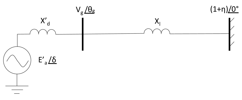
Figure 1: Stochastic single machine infinite bus system used in Sec. III. The notation $V_{g}\phase{\theta_{g}}$ represents $V_{g}\exp\left[j\theta_{g}\right]$.

III-B Autocorrelation and Variance

In this section, we calculate the autocorrelations and variances of the algebraic and differential variables of this system using the method in Sec. II. Equations (1) and (2) describe this system for which the following equalities hold:

$$\gamma=\frac{D}{2M};\omega_{0}=\sqrt{\frac{E_{a}^{{}^{\prime}}\cos\delta_{0}}{MX}};\underline{y}=\left[\begin{array}[]{cc}V_{g}&\theta_{g}\end{array}\right]^{T}$$ (30)

$$f=\frac{P_{g0}}{M};F_{1}\left(z,\underline{y},\eta\right)=\left(\frac{(1+\eta)E_{a}^{{}^{\prime}}}{X}\sin\delta-P_{m}\right)/M$$ (31)

where $\Delta V_{g}=V_{g}-V_{g0},\Delta\theta_{g}=\theta_{g}-\theta_{g0}$ are the deviations of, respectively the generator terminal busbar’s voltage magnitude and angle from their equilibrium values. Equations (30) and (31) show that $f$ increases with $\delta_{0}$ while $\omega_{0}$ decreases with $\delta_{0}$.

In order to calculate the algebraic equations, which form $\underline{F_{2}}\left(\delta,y,\eta\right)$ in (2), we wrote Kirchhoff’s current law at the generator’s terminal:

$$\frac{E^{\prime}_{a}e^{j\delta}-V_{g}e^{j\theta_{g}}}{jX^{\prime}_{d}}+\frac{1+\eta-V_{g}e^{j\theta_{g}}}{jX_{l}}=0$$ (32)

Separating the real and imaginary parts in (32) gives the following:

$$V_{g}\sin\left(\theta_{g}\right) = \alpha E_{a}^{{}^{\prime}}\sin\left(\delta\right)$$ (33)

$$V_{g}\cos\left(\theta_{g}\right) = \alpha E_{a}^{{}^{\prime}}\cos\left(\delta\right)$$

$$+\left(1+\eta\right)\left(1-\alpha\right)$$

where $\alpha=X_{l}/(X_{l}+X_{d}^{{}^{\prime}})$. Equations (33) and (III-B) combine to make $\underline{F_{2}}\left(\delta,y,\eta\right)$ in (2).

Linearizing (33) and (III-B) yields the coefficients in (21), which are necessary for calculating the autocorrelations and variances of the algebraic variables (here $y_{1}=\Delta V_{g},y_{2}=\Delta\theta_{g}$):

$$C_{1_{,}1} = \alpha E_{a}^{{}^{\prime}}\sin\left(\theta_{g0}-\delta_{0}\right)$$ (35)

$$C_{1_{,}2} = \left(1-\alpha\right)\cos\left(\theta_{g0}\right)$$ (36)

$$C_{2_{,}1} = \alpha E_{a}^{{}^{\prime}}\cos\left(\theta_{g0}-\delta_{0}\right)$$ (37)

$$C_{2_{,}2} = -\left(1-\alpha\right)\sin\left(\theta_{g0}\right)$$ (38)

Fig. 2 shows the decrease of $\omega^{\prime}$, which is the absolute value of the imaginary part of the eigenvalues of $A$ in (9), with $P_{m}$. Note that the bifurcation occurs at $P_{m}=5\textrm{{pu}}$. This figure illustrates how it can be difficult to accurately foresee a bifurcation by computing the eigenvalues of a system (as in, e.g., [19]), if there is noise in the measurements feeding the calculation. The value of $\omega^{\prime}\sim\left(P_{m}-\textrm{{b}}\right)^{1/4}$ does not decrease by a factor of two (compared to its value at $P_{m}=1.0\textnormal{{pu}}$) until $P_{m}=4.83\textrm{{pu}}$ (only $<3.4\%$ away from the bifurcation). It decreases by another factor of two at $P_{m}=4.99\textrm{{pu}}$ ($0.2\%$ away from the bifurcation). Also, note that the real part of the eigenvalues are equal to $-\gamma$ until very close to the bifurcation ($0.1\%$ away from the bifurcation), so they do not provide a useful indication of proximity to the bifurcation. Thus, one can confidently predict from $\omega^{\prime}$ the imminent occurrence of the bifurcation only very near it, which may be too late to avert it. On the other hand, we will demonstrate below that for this system, autocorrelation functions can provide substantially more advanced warning of the bifurcation.

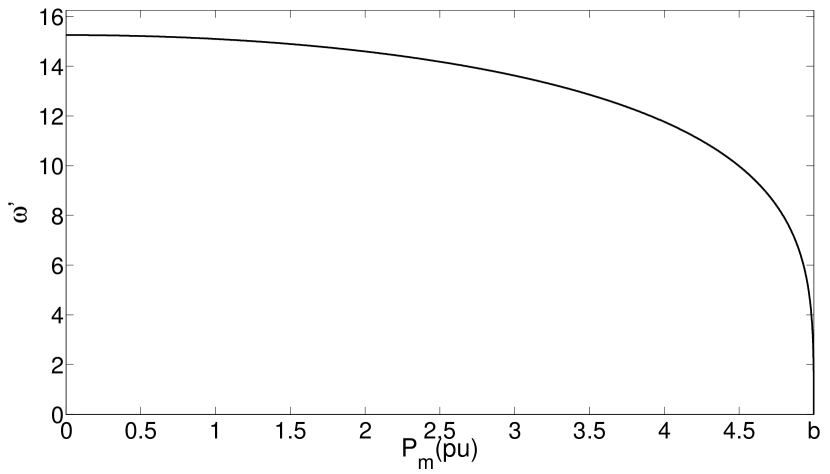
Figure 2: The decrease of $\omega^{\prime}$ with $P_{m}$ in the SMIB system. Near the bifurcation, $\omega^{\prime}$ is very sensitive to changes in $P_{m}$. In this figure, and most that follow, b is the value of the bifurcation parameter ($P_{m}$ in this system) at the bifurcation.

Using autocorrelation as an early warning sign of potential bifurcations requires that one carefully select a time lag, $\Delta t=t-s$, such that changes in autocorrelation are observable. To understand the impact of different time lags, we computed the autocorrelation as function of $\Delta\delta$ (see Fig. 3). From (II-B), the autocorrelation of $\delta(t)$ crosses zero at $\Delta t_{0}=\frac{2\pi-\phi}{\omega^{\prime}}$. The implication is that choosing $\Delta t$ close to $\Delta t_{0}$ allows one to observe a monotonic increase of autocorrelation as $P_{m}$ increases. For $\Delta t>\Delta t_{0}$, autocorrelation may not increase monotonically, or the autocorrelation for some values of $P_{m}$ may be negative. For example, in Fig. 3 for $\Delta t=0.3\textrm{{s}}$, the autocorrelation decreases first and then increases with $P_{m}$. On the other hand, for $\Delta t$ considerably smaller than $\Delta t_{0}$, the increase of the autocorrelation may not be large enough to be measurable. In Fig. 3, the curves converge as $\Delta t\rightarrow 0$. Given that the smallest period of oscillation $(T=2\pi/\omega^{\prime})$ in this system is $0.41\textrm{s}$, we chose $\Delta t=0.1$s for the autocorrelation calculations in this section.

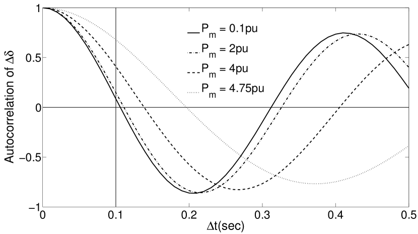
Figure 3: Autocorrelation function of $\Delta\delta$. $\Delta t=0.1$s is close to 1/4 of the smallest period of the function for all values of $P_{m}$.

Using (16)–(II-B), we calculated the variances and autocorrelations of $\Delta\delta$, $\Delta\dot{\delta}$ at different operating points. In Figs. 4 and 5, these analytical results are compared with the numerical ones. To initialize the numerical simulations, we assumed that $V_{g0}=1\textrm{{pu}}$ and solved for $E^{\prime}_{a}$ in (33), (III-B) to obtain $V_{g}=V_{g0}$ (for $\eta=0$). We chose the integration step size $\tau_{int}$ to be 0.01s, which is much shorter than the the smallest period of oscillation ($T=0.41\textrm{s}$). The numerical results are shown for the range of bifurcation parameter values for which the numerical solutions were stable.

In order to determine if variance and autocorrelation measurably increase as load approaches the bifurcation, we computed the ratio of each statistic when load is at 80% of the bifurcation value to the value when load is at 20% of b. This ratio, $q_{\frac{80}{20}}$ in Figs. 4 and 5, is defined as follows:

$$q_{\frac{80}{20}}=\frac{\textrm{Autocorrelation}\textrm{ {of} }u\textrm{ or }\sigma_{u}^{2}|_{P_{m}=0.8b}}{\textrm{Autocorrelation}\textrm{ {of} }u\textrm{ or }\sigma_{u}^{2}|_{P_{m}=0.2b}}$$ (39)

where $u$ is the plot’s variable. In subsequent figures, $q_{\frac{80}{20}}$ is defined similarly.

Fig. 4 shows that the variances of both $\Delta\delta$ and $\Delta\dot{\delta}$ increase substantially with $P_{m}$, and thus appear to be good warning signs of the bifurcation. However, the two variances grow with different rates. (This becomes clear when comparing the ratios $q_{\frac{80}{20}}$ for $\Delta\delta$ and $\Delta\dot{\delta}$.) The difference becomes even more noticeable near the bifurcation where the variance of $\Delta\delta$ increases much faster than the variance of $\Delta\dot{\delta}$. This is caused by the term $\omega_{0}^{2}$ in the denominator of the expression for the variance of $\Delta\delta$ in (16). In Fig. 5, the autocorrelations of $\Delta\delta$ and $\Delta\dot{\delta}$ increase with $P_{m}$. Similar to the variances, the autocorrelations are good early warning signs of the bifurcation as well. Comparing Figs. 4 and 5 with Fig. 2 (where an equivalent $q_{\frac{80}{20}}$ would be 1.28) shows that the autocorrelations and variances of $\Delta\delta$ and $\Delta\dot{\delta}$ provide a substantially stronger early warning sign, relative to using eigenvalues to estimate the distance to bifurcation in this system.

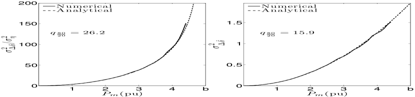
Figure 4: Variances of $\Delta\delta,\Delta\dot{\delta}$ versus mechanical power $(P_{m})$ values.

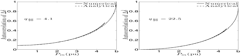
Figure 5: Autocorrelations of $\Delta\delta,\Delta\dot{\delta}$ versus mechanical power $(P_{m})$ values. The autocorrelation values are normalized by dividing by the variances of the variables.

The results for the algebraic variables are mainly similar. Figs. 6,7 show the variances and autocorrelations of $\Delta V_{g},\Delta\theta_{g}$ as a function of load. In Fig. 6, the variance of $\Delta V_{g}$ decreases with $P_{m}$ until the system gets close to the bifurcation, while the variance of $\Delta\theta_{g}$ increases with $P_{m}$ even if the system is far from the bifurcation. The autocorrelations of both $\Delta V_{g}$ and $\Delta\theta_{g}$ in Fig. 7 increase with $P_{m}$. However, the ratio $q_{\frac{80}{20}}$ in (39) is much larger for $\Delta V_{g}$ than for $\Delta\theta_{g}$. This is caused by the autocorrelation of $\Delta V_{g}$ being very close to zero for small values of $P_{m}$.

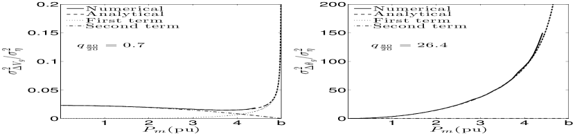
Figure 6: Variances of $\Delta V_{g}$ and $\Delta\theta_{g}$ versus mechanical power $\left(P_{m}\right)$ levels. The two terms comprising the variances in (25) are also shown.

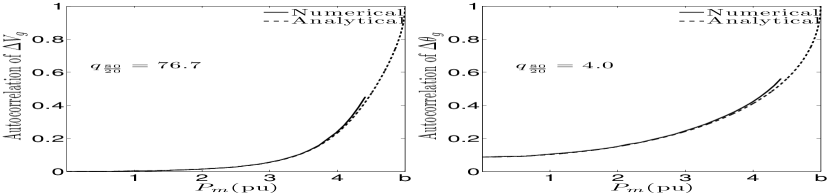
Figure 7: Autocorrelations of $\Delta V_{g}$ and $\Delta\theta_{g}$ versus $P_{m}$.

III-C Discussion

These results can be better understood by observing the trajectory of the eigenvalues of the SMIB system (Fig. 8). Near the bifurcation, the eigenvalues are very sensitive to changes in the bifurcation parameter. As a result, the system is in the overdamped regime $(\omega_{0}<\gamma)$ for much less than 0.1% distance in terms of $P_{m}$ to the critical transition. This implies that, at least for this system, the autocorrelation function in [7, 8], is valid only when the system is within $0.1\%$ of the saddle-node bifurcation. Because the method in [7, 8] can provide a good estimate of the autocorrelations and variances of state variables only for a very short range of the bifurcation parameter, it may not be particularly useful as an early warning sign of bifurcation.

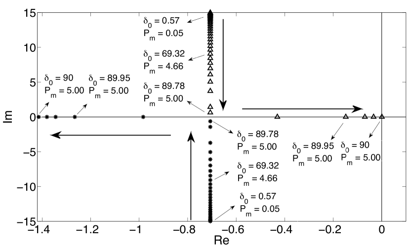
Figure 8: Eigenvalues of the first system as the bifurcation parameter (mechanical power) is increased. The arrows show the direction of the eigenvalues’ movement in the complex plane as $P_{m}$ is increased. The values of $P_{m}$ and $\delta_{0}$ are given for several eigenvalues.

From Figs. 4–7, we can observe that, except for the variance of $\Delta V_{g}$, the variances and autocorrelations of all state variables increase when the system is more loaded. This demonstrates that CSD occurs in this system as it approaches bifurcation, as suggested both by general results [9], and prior work for power systems [6, 7].

In addition to validating these prior results, several new observations can be made. For example, the signs of CSD are more clearly observable in some variables than in others. While all of the variables show some increase in autocorrelation and variance, they are less clearly observable in $\Delta V_{g}$. The variance of $\Delta V_{g}$ decreases with $P_{m}$ slightly until the vicinity of the bifurcation. In comparison, the variance of $\Delta\theta_{g}$ always increases with $P_{m}$. Fig. 6 shows the two terms of the expressions for the variances of $\Delta V_{g}$ and $\Delta\theta_{g}$ in (25). The second term of the variance of $\Delta\theta_{g}$ is very small compared to the first term, and the first term is always dominant and growing. On the other hand, the second term of the variance of $\Delta V_{g}$ is more significant for small $P_{m}$. This term decreases with $P_{m}$, which can be observed from the expression for $C_{1_{,}2}$ in (36). Accordingly, decrease of $C_{1_{,}2}$ with $P_{m}$ causes the the variance of $\Delta V_{g}$ to decrease with $P_{m}$ until the vicinity of the bifurcation. In conclusion, the variance of $\Delta\theta_{g}$ is a better indicator of proximity to the bifurcation. Because the variables $\Delta\delta$ and $\Delta\dot{\delta}$ are highly correlated with $\Delta\theta_{g}$, their variances are also good indicators of proximity to the bifurcation.

The rate at which autocorrelation increases with $P_{m}$ differs significantly in Figs. 5 and 7. In Fig. 5, the ratio $q_{\frac{80}{20}}$ in (39) is 5.5 times larger for $\Delta\dot{\delta}$ than for $\Delta\delta$. The normalized autocorrelation functions of $\Delta\delta$ and $\Delta\dot{\delta}$ are as follows:

$$\textnormal{{E}}\left[\Delta\delta\left(t\right)\Delta\delta\left(s\right)\right]/\sigma_{\Delta\delta}^{2} = \exp\left(-\gamma\Delta t\right)\frac{\omega_{0}}{\omega^{\prime}}$$

$$\cdot\sin\left(\omega^{\prime}\Delta t+\phi\right)$$

$$\textnormal{{E}}\left[\Delta\dot{\delta}\left(t\right)\Delta\dot{\delta}\left(s\right)\right]/\sigma_{\Delta\dot{\delta}}^{2} = \exp\left(-\gamma\Delta t\right)\frac{\omega_{0}}{\omega^{\prime}}$$

$$\cdot\sin\left(\omega^{\prime}\Delta t+\pi-\phi\right)$$

The difference between the two functions is in the phase of the sine function which causes the values of the two autocorrelations to be different. $q_{\frac{80}{20}}$ is so much larger for $\Delta\dot{\delta}$ than for $\Delta\delta$ because of the time lag ($\Delta t$) used to compute autocorrelation. $\Delta t=0.1\mbox{s}$ is close to the zero crossing of the autocorrelation function of $\Delta\dot{\delta}$, causing the large $q_{\frac{80}{20}}$. This difference illustrates the importance of choosing an appropriate time lag.

It is important to note that although the growth ratio of the autocorrelation for $\Delta\delta$ is not large compared to $\Delta\dot{\delta}$, it can be increased by subtracting a bias value from the autocorrelation values for $P_{m}=0.2b(\textrm{{pu})}$ and $P_{m}=0.8b\textrm{({pu}})$. For example, if the value of 0.075 is subtracted from the autocorrelation values, the ratio $q_{\frac{80}{20}}$ increases from 4.1 to 13.0. When using this approach, it is recommended that the new base value (here, autocorrelation of $\Delta\delta$ for $P_{m}=0.2\textrm{b}(\textrm{{pu})}$) is chosen to be at least $25\%$ of the original value, in order to reduce the impact of measurement noise.

The results also show that it is the nonlinearity of this system that causes CSD to occur. One of the elements of the state matrix $(-\omega_{0}^{2})$ in (9) changes with $P_{m}$ because of the nonlinear relationship between the electrical power $(P_{g})$ and the rotor angle, causing the eigenvalues to change with $P_{m}$. If the relationship between $P_{g}$ and $\delta$ were linear, the state matrix $A$ would be constant. Indeed, in [31], it is shown that the stationary time correlation matrix of (6) can be calculated using the following equation:

$$\textnormal{{E}}\left[\mathbf{\mathbf{\underline{\mathrm{\mathit{Z}}}\left(\mathit{t}\right)}}\underline{Z}{}^{T}\left(s\right)\right]=\exp\left[-A\Delta t\right]\sigma$$ (42)

where $\sigma$ is the covariance matrix of the state variables. Thus, the normalized autocorrelation matrix depends only on $A$ and the time lag. As a result, if the state matrix is constant, the autocorrelation for a specific time lag will also be constant. Thus, in this system, CSD is caused by the nonlinear relationship between $P_{g}$ and the rotor angle.

IV Single Machine Single Load System

The first system illustrates how CSD can occur in a generator connected to a large power grid, through a long line. In this section we use a generator to represent the bulk grid, and look for signs of CSD caused by a stochastically varying load. Some form of the single machine single load (SMSL) model used in this section has been used extensively to study voltage collapse (e.g., [13, 39]).

IV-A Stochastic SMSL System Model

The second system (shown in Fig. 9) consists of one generator, one load and a transmission line between them. The random variable $\eta$ defined in (3) and (4), is added to the load to model its fluctuations. The load consists of both active and reactive components. In order to stress the system, the baseline load $S_{d}$ is increased, while keeping the noise intensity ($S_{d0}$) and the load’s power factor constant.

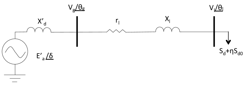
Figure 9: Single machine single load system.

A set of differential-algebraic equations comprising the swing equation and power flow equations describe this system. The swing equation and the generator’s electrical power equation are given below:

$$M\ddot{\delta}+D\dot{\delta} = P_{m}-P_{g}$$ (43)

$$P_{g} = E_{a}^{{}^{\prime}}V_{l}G_{gl}\cos\left(\delta-\theta_{l}\right)$$

$$+E_{a}^{{}^{\prime}}V_{l}B_{gl}\sin\left(\delta-\theta_{l}\right)+E_{a}^{{}^{\prime}2}G_{gg}$$

where $V_{l},\theta_{l}$ are voltage magnitude and angle of the load busbar, $G_{gl},G_{gg}$ and $B_{gl}$ are as follows:

$$G_{gg} = -G_{gl}=\textrm{$\mathsf{{Re}}$}\left(\frac{1}{r_{l}+jX_{l}}\right)$$ (45)

$$B_{gl} = \mathsf{-{Im}}\left(\frac{1}{r_{l}+jX_{l}}\right)$$ (46)

The power flow equations at the load bus are as follows:

$$-P_{d}-P_{d0}\eta = V_{l}E_{a}^{{}^{\prime}}G_{gl}\cos\left(\theta_{l}-\delta\right)$$

$$+V_{l}E_{a}^{{}^{\prime}}B_{gl}\sin\left(\theta_{l}-\delta\right)+V_{l}^{2}G_{ll}$$

$$-Q_{d}-Q_{d0}\eta = V_{l}E_{a}^{{}^{\prime}}G_{gl}\sin\left(\theta_{l}-\delta\right)$$

$$-V_{l}E_{a}^{{}^{\prime}}B_{gl}\cos\left(\theta_{l}-\delta\right)-V_{l}^{2}B{}_{ll}$$

where $G_{ll}=G_{gg},\,B_{ll}=-B_{gl}$, and $P_{d0},Q_{d0}$ are constant values. The parameters of this system are similar to the SMIB system, with the following additional parameters: $r_{l}=0.025\Omega,P_{d0}=1\textrm{pu}$, $pf=0.95\textrm{{lead}}$, where $r_{l}$ is the line’s resistance and $pf$ is the load’s power factor.

In this system, $V_{l}$, $\theta_{l}-\delta$ are the algebraic variables, and $\delta$, $\dot{\delta}$ are the differential variables. The algebraic equations (IV-A) and (IV-A) define $V_{l}$ and $\theta_{l}-\delta$, which then drive $\delta$ through (43) and (IV-A). By linearizing (IV-A) and the power flow equations around the equilibrium, we simplified (43) to the following:

$$\Delta\ddot{\delta}+\frac{D}{M}\Delta\dot{\delta}=-\frac{C_{5}}{M}\eta$$ (49)

where $C_{5}$ is a function of the system state at the equilibrium point. The derivation of (49) and the expression for $C_{5}$ are presented in Appendix A. Comparing (5) with (49) yields the following:

$$\gamma=\frac{D}{2M},\omega_{0}=0,f=\frac{C_{5}}{M}$$ (50)

The expression for the autocorrelation of $\Delta\dot{\delta}$ is given in (20). Note that the normalized autocorrelation of $\Delta\dot{\delta}$ does not change with the bifurcation parameter $(P_{d})$, as it did for the SMIB system. In Appendix A, it is shown that $\Delta V_{l}$ and $\Delta\delta-\Delta\theta_{l}$ are proportional to $\eta$ (see (58) and (59)). As a result, they are memoryless; the variables have zero autocorrelation.

Figs. 10 and 11 show the analytical and numerical solutions of the variances of $\Delta\dot{\delta}$, $\Delta V_{l}$ and $\Delta\delta-\Delta\theta_{l}$. Unlike the SMIB system, the variance of $\Delta V_{l}$ is a good early warning sign of the bifurcation. It is also much more sensitive to the increase of $P_{d}$ compared to $\Delta\delta-\Delta\theta_{l}$ and $\Delta\dot{\delta}$.

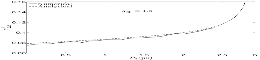
Figure 10: Variance of $\Delta\dot{\delta}$ for different load levels. The variance increases modestly with $P_{d}$ as the system approaches the bifurcation.

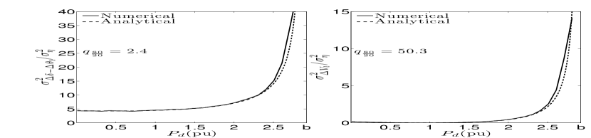
Figure 11: Variances of $\Delta\delta-\Delta\theta_{l}$ and $\Delta V_{l}$ for different load levels. Both variances increase with $P_{d}$ as the system approaches the bifurcation.

IV-B Discussion

As was the case with the SMIB system, when the power flowing on the transmission line in this system reaches its transfer limit, the algebraic equations become singular. However, unlike the previous system, the differential equations of this system do not become singular at the bifurcation point of the algebraic equations. Fig. 12 shows the sample trajectories of the two systems’ rotor angles. Both signals are Gaussian stochastic processes. The rotor angle in the SMIB system is an Ornstein–Uhlenbeck process while the rotor angle in the SMSL system varies like the position of the brownian particle [40]. The existence of the infinite bus in the former system causes this difference.

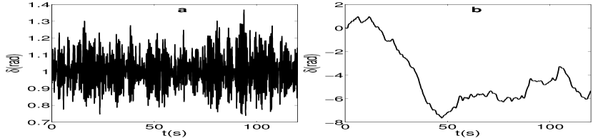
Figure 12: A sample trajectory of the rotor angle of (a) the SMIB system (b) the SMSL system.

One difference between the SMSL system and the SMIB system is the absence of the term comprising $\Delta\delta$ in (49) compared with (5). This causes the linearized state matrix to be independent of the bifurcation parameter. From (42), one can show that the normalized autocorrelation of $\Delta\dot{\delta}$ depends only on $A$ and the time lag. Since $A$ is constant in this system, the autocorrelation of $\Delta\dot{\delta}$ will be constant for a specific $\Delta t$.

The increase of the variances of both differential and algebraic variables is due to the non-linearity of the algebraic equations. Fig. 13 shows that as the load power increases, the perturbation of the load power causes a larger deviation in the load busbar voltage magnitude. Consequently, variance of this algebraic variable increases with $P_{d}$. Likewise, this nonlinearity causes the coefficient $C_{5}$ in (49) to increase as the load power is increased, increasing the variance of $\Delta\dot{\delta}$. One can show that if the line resistance ($r_{l}$) is neglected in this system, $C_{5}$ in (49) will be replaced by $P_{d0}$. In this case, the variance of $\Delta\dot{\delta}$ is constant, since the differential and algebraic equations are fully decoupled.

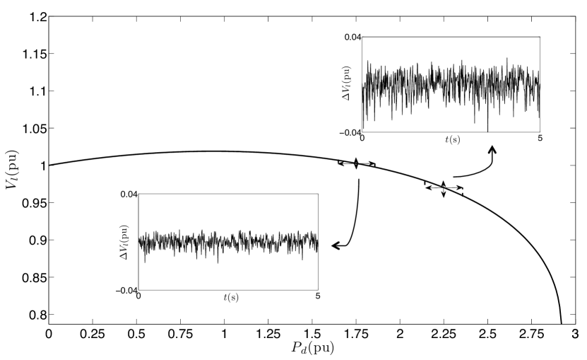
Figure 13: The load bus voltage as a function of load power. The load bus voltage magnitude becomes increasingly sensitive to power fluctuations as the system approaches the bifurcation. This increased sensitivity raises the voltage magnitude’s variance.

While voltage variance increases with load, this system does not technically show CSD before the bifurcation, since increases in both variance and autocorrelation are essential to conclude that CSD has occurred [9]. Also, the eigenvalues of the state matrix of this system do not vary with load. This confirms that CSD does not occur in this system, since the poles of the dynamical system do not move toward the right-half plane as the bifurcation parameter increases [1], [9].

V Three-Bus System

Real power systems have properties that are common to both the SMIB in Sec. III and the SMSL in Sec. IV. In order to explore CSD for a system that has both an infinite bus, and the potential for voltage collapse case, this section looks at the three-bus system in Fig. 14.

V-A Model and Results

The three-bus system consists of a generator connected to a load bus through a transmission line, which is connected to an infinite bus through another transmission line. In the SMIB system, the bifurcation occurred in the differential equations. Increasing the load in the three-bus system causes a saddle-node bifurcation in the algebraic equations $F_{1}\left(\delta,\underline{y},0\right)=0,\underline{F_{2}}\left(\delta,\underline{y},0\right)=0$ (in terms of (1), (2)), as in the SMSL system. However, unlike in the SMSL system, the bifurcation in these algebraic equations also causes a bifurcation in the differential equation (5).

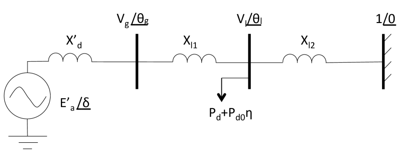
Figure 14: Three–bus system.

We studied this system for two different cases. Our goal from studying these two cases was to show that the CSD signs for some variables can vary differently with changing the system parameters. In case A, the parameters of this system are similar to those in the SMIB system except for the following:

$X_{l1}=\textrm{0.1{pu}},X_{l2}=0.35\textrm{pu},X^{\prime}_{d}=0.1\textrm{pu}$

In Case B, the following parameters were used:

$X_{l1}=\textrm{0.3{pu}},\,D=0.001\frac{\textnormal{{pu}}}{rad/s}$

The algebraic equations of the three-bus system are as follows:

$$\left(\frac{E^{\prime}_{a}V_{l}}{X}\sin\left(\delta-\theta_{l}\right)-\frac{2}{3}P_{d}\right)/M = 0$$ (51)

$$\frac{E^{\prime}_{a}V_{l}}{X}\sin\left(\delta-\theta_{l}\right)-\frac{V_{l}}{X_{l2}}\sin\left(\theta_{l}\right)-P_{d0}\eta = P_{d}$$ (52)

$$\frac{E^{\prime}_{a}V_{l}}{X}\cos\left(\delta-\theta_{l}\right)+\frac{V_{l}}{X_{l2}}\cos\left(\theta_{l}\right) = V_{l}^{2}\cdot$$

$$\left(\frac{1}{X}+\frac{1}{X_{l2}}\right)$$

where $X=X_{d}^{{}^{\prime}}+X_{l1}$, $V_{l},\theta_{l}$ are voltage magnitude and angle of the load busbar. Equation (51) is equivalent to $F_{1}\left(\delta,\underline{y},0\right)$ in (1), and (52), (V-A), which are the simplified active and reactive power flow equations at the load busbar, are equivalent to $F_{2}\left(\delta,\underline{y},0\right)$ in (2). We assumed that $P_{g0}=\nicefrac{{2P_{d}}}{{3}}$, which is reflected in (51).

The following equalities relate this system to the general model in (5):

$$\gamma=\frac{D}{2M};\omega_{0}^{2}=\frac{-C_{6}}{M};f=\frac{-C_{7}}{M}$$ (54)

where $C_{6}$ and $C_{7}$ are functions of the system state at the equilibrium point. The derivation and expressions for $C_{6},C_{7}$ are presented in Appendix B. Fig. 15 shows $C_{6},C_{7}$ versus $P_{d}$. When the load increases, $C_{6}$ approaches $0,$ and a bifurcation in the differential equation (5) and (54) occurs.

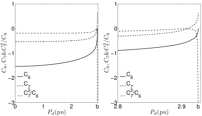
Figure 15: Three variables $C_{6},C_{7}$ and $C_{7}^{2}/C_{6}$ derived by linearizing the Three-bus system model. The left panel shows the variables versus $P_{d}$ for Case B. The right panel shows a close-up view of the variables near the bifurcation. Note that as $P_{d}\rightarrow P_{d,cr}$, $C_{6}\rightarrow 0$ while $C_{7}$ approaches a finite value of $\sim 0.6$. $C_{7}^{2}/C_{6}\rightarrow\infty$, as $P_{d}\rightarrow P_{d,cr}$.

Using (54), the expressions in Sec. II-B, and (76), (77) in Appendix B, we calculated the variances and autocorrelations of $\Delta\delta,\Delta\dot{\delta},\Delta V_{l}$ and $\Delta\theta_{l}$. We chose the autocorrelation time lag $\Delta t$ of the variables to be equal to 0.14s taking a similar approach as in Sec. III-B. Although the chosen $\Delta t$ may not be optimal for all of the variables, it represents a reasonable compromise between simplicity (choosing just one $\Delta t$) and usefulness as early warning signs. Figs. 16–19 compare the analytical solutions with the numerical solutions of the variances and autocorrelations of $\Delta\delta$, $\Delta\dot{\delta}$, $\Delta V_{l}$ and $\Delta\theta_{l}$.

Fig. 17 shows that although the growth rates of the autocorrelations of $\Delta\delta,\Delta\dot{\delta}$ are not large, the autocorrelations increase monotonically in both cases. As mentioned in Sec. III-C, it is possible to have larger indicators (growth ratios) by subtracting a bias value from the autocorrelations. On the other hand, the variances of $\Delta\delta,\Delta\dot{\delta}$ in Fig. 16, do not monotonically increase for case B. We will explain this behavior in the next subsection. As a result, they are not reliable indicators of proximity to the bifurcation.

Fig. 18 shows that although both variances of $\Delta V_{l}$ and $\Delta\theta_{l}$ increase with $P_{d}$, increase of the variance of $\Delta V_{l}$ is more significant. Also, the variance of $\Delta\theta_{l}$ does not increase monotonically with $P_{d}$ for case B. As a result, the variance of $\Delta V_{l}$ seems to be a better indicator of the system stability.

In Fig. 19, the autocorrelation of $\Delta V_{l}$ until very near the bifurcation is small compared to those in Fig. 17. This is caused by $C_{26}$ being very small in (76), so $\Delta V_{l}$ is tied to the differential variables weakly. As a result, $\Delta V_{l}$ behaves in part like $\eta$—the white random variable, and hence its autocorrelation is not a good indicator of proximity to the bifurcation. In addition, nonmonotonicity of the autocorrelations of $\Delta V_{l},\,\Delta\theta_{l}$ for case B in Fig. 19 shows that they are not good early warning signs of bifurcation.

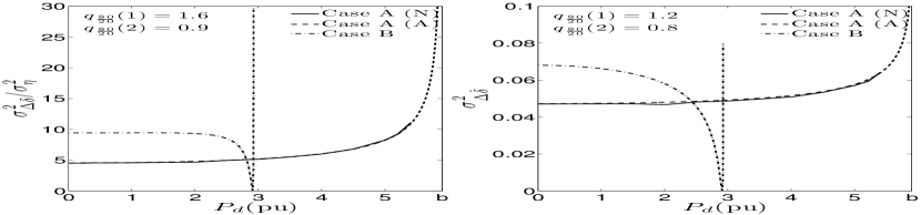
Figure 16: Variances of $\Delta\delta,\Delta\dot{\delta}$ versus load power $\left(P_{d}\right)$. The ratios $q_{\frac{80}{20}}(1),q_{\frac{80}{20}}(2)$ are for case A, case B respectively. CaseA(N), CaseA(A) denote numerical and analytical solutions for case A.

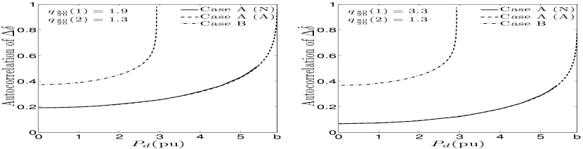
Figure 17: Autocorrelations of $\Delta\delta,\Delta\dot{\delta}$ versus $\textrm{P}_{d}$. Both of the autocorrelations increase with $P_{d}$.

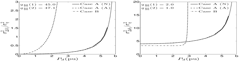
Figure 18: Variances of $\Delta V_{l},\Delta\theta_{l}$ versus $P_{d}$.

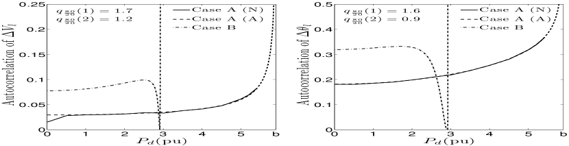
Figure 19: Autocorrelations of $\Delta V_{l},\Delta\theta_{l}$ versus $\textrm{P}_{d}$.

V-B Discussion

After studying this system with a range of different parameters, we found that autocorrelations of the differential variables and variance of the voltage magnitude are consistently good indicators of proximity to the bifurcation.

On the other hand, as shown in Fig. 16, variance in the differential variables is not a reliable indicator. Namely, variances change non-monotonically (i.e., they do not always increase) and, importantly, may exhibit very abrupt changes. Fig. 15 provides some clues as to the reason for this latter phenomenon. In this figure, the absolute value of $C_{7}$ decreases with $P_{d}$ and becomes zero very close to the bifurcation point, at $P_{d|C_{7}=0}$. Therefore, the variances of $\Delta\delta$ and $\Delta\dot{\delta}$, which are proportional to $C_{7}^{2}$, decrease and vanish at $P_{d|C_{7}=0}$. Past this point, $\left|C_{7}\right|$ increases, while $C_{6}$ continues to decrease and vanishes at $b$. Therefore, the variances of $\Delta\delta$ and $\Delta\dot{\delta}$, which are proportional to $\nicefrac{{C_{7}^{2}}}{{C_{6}}}$, increase to infinity in the very narrow interval $\left(P_{d|C_{7}=0},\,b\right)$; see Fig. 15. This explains the sharp features in Fig. 16; a similar explanation can be given to such a feature in Fig. 19. Therefore, neither the variances of $\Delta\delta,\Delta\dot{\delta}$ or the autocorrelations of $\Delta V_{l},\Delta\theta_{l}$ are good indicators of proximity to bifurcation.

The results for this system clearly show that not all of the variables in a power system will show CSD signs long before the bifurcation. Although autocorrelations and variances of all variables increase before the bifurcation, some of them increase only very near the bifurcation or the increase is not monotonic. Hence, these variables are not useful indicators of proximity to the bifurcation. In the three-bus system, autocorrelation in the differential equations was a better indicator of proximity than autocorrelation in $\Delta V_{l}$ or $\Delta\theta_{l}$, which are not directly associated with the differential equations. Also, $\Delta V_{l}$ was the only variable whose variance shows a gradual and monotonic increase with the bifurcation parameter.

VI CSD in multi-machine systems

In order to compare these analytical results to results from more practical power system, this section presents numerical results for two multi-machine systems.

The first system was similar to the Three-bus system (case B in Sec. V). The only difference was that instead of infinite bus, a generator similar to the other generator was used. The numerical simulation results were similar to the Three-bus system, except for the autocorrelation of $\Delta\dot{\delta}$. Fig. 20 shows that autocorrelation of $\Delta\dot{\delta}$ increases for one of the machines, while it decreases for the other one. This shows that the autocorrelation of $\Delta\dot{\delta}$ is not a reliable indicator of the proximity to the bifurcation.

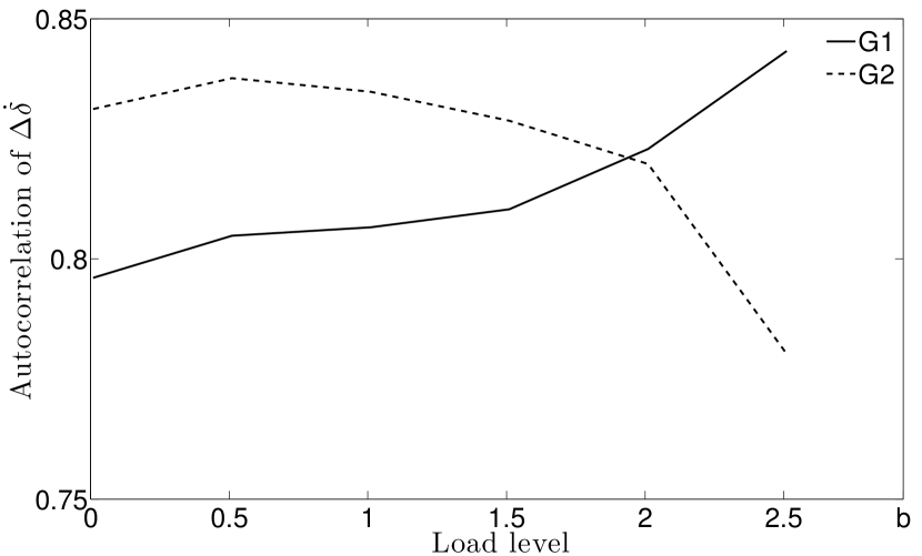
Figure 20: Autocorrelation of $\Delta\dot{\delta}$ for two machines in the Three-bus system with two generators. $G_{1}$ is the same generator as in the Three-bus system and $G_{2}$ is the new generator.

The second system we studied was the New England 39-bus system, using the system data from [41] We simulated this system for different load levels using the power system analysis toolbox (PSAT) [42]. Exciters and governors were not included in the results here, although subsequent tests indicate that adding them do not substantially change the conclusions. In order to change the system loading, each load was multiplied by the same factor. At each load level, we added white noise to each load. As one would expect, increasing the loads moves the system towards voltage collapse. For solving the stochastic DAEs, we used the fixed-step trapezoidal solver of PSAT with the step size of 0.01s. The noise intensity was kept constant for all load levels.

The simulation results show that the variances and autocorrelations of bus voltage magnitudes increase with load. However, similar to the Three-bus system, the autocorrelations of voltage magnitudes are very small, indicating that in practice, these variables would not be good indicators of proximity. The variances and autocorrelations of generator rotor angles and speeds and bus voltage angles did not consistently show an increasing pattern. Figs. 21 and 22 show the variances and autocorrelations of the voltage magnitudes of five busbars and the rotor angles of five generators of the system respectively. The buses and generators were arbitrarily chosen. As in previous results, the autocorrelation time lag was chosen to be 0.1s.

The results in this section suggest that autocorrelations of differential variables show nonmonotic behavior in some cases, which limits their application as early waning signs of bifurcation.

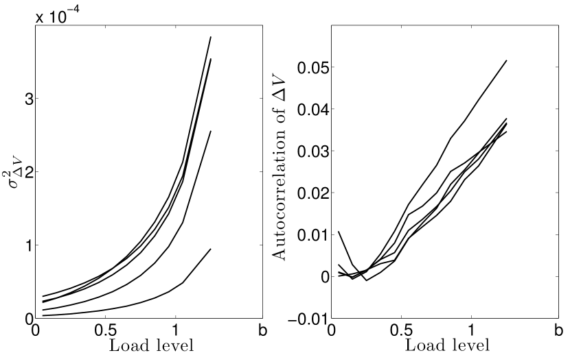
Figure 21: The variances and autocorrelations of the voltage magnitudes of five busbars of the system. Load level is the ratio of the values of the system’s loads to their nominal values.

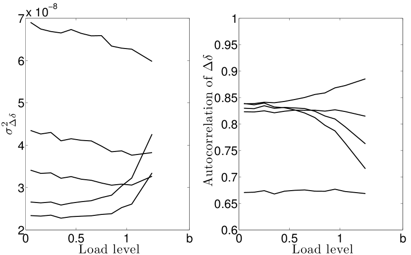
Figure 22: The variances and autocorrelations of the rotor angles of five generators of the system.

In many ways, this test case is a multi-machine version of the SMSL system. As with the SMSL and Three-bus systems, variances of bus voltage magnitudes are good early warning signs. However, unlike in the SMSL system, autocorrelation in voltage magnitudes increases, albeit only slightly, with system load. Unlike in the SMSL system, voltage magnitudes in the 39-bus case have non-zero autocorrelation for $\Delta t>0$. This results from the fact that voltage magnitudes are coupled to the differential variables in this system.

Results from this system, as with the SMSL system, suggest that variance in voltage magnitudes is a useful early warning sign of voltage collapse. It is less clear from these results if changes in autocorrelation will be sufficiently large to provide a reliable early warning of criticality.

VII Conclusion

In this paper, we analytically and numerically solve the stochastic differential algebraic equations for three small power system models in order to understand critical slowing down in power systems. The results from the single machine infinite bus system and the Three-bus system models show that critical slowing down does occur in power systems, and illustrate that autocorrelation and variance in some cases can be good indicators of proximity to criticality in power systems. The results also show how non-linear dynamics influence the observed changes in autocorrelation and variance. For example, linearity of the differential equation in the single machine single load system caused the autocorrelation of the differential variable to be constant. On the other hand, in the SMIB system and Three-bus system, the differential equations were nonlinear and autocorrelations of the differential variables increased with the bifurcation parameter.

Although the signs of critical slowing down do consistently appear as the systems approach bifurcation, only in a few of the variables did the increases in autocorrelation appear sufficiently early to give a useful early warning of potential collapse. On the other hand, variance in load bus voltages consistently showed substantial increases with load, indicating that variance in bus voltages can be a good indicator of voltage collapse in multi-machine power system models. This was verified for the New England 39-bus system.

Together these results suggest that it is possible to obtain useful information about system stability from high-sample rate time-series data, such as that produced by synchronized phasor measurement units. Future research will focus on developing an effective power system stability indicator based on these results.

Appendix A

The derivation of (49) is presented in this section. By linearizing (IV-A) around the equilibrium and replacing the obtained equation for $P_{g}$ in (43), we obtained the following:

$$M\Delta\ddot{\delta}+D\Delta\dot{\delta}=-C_{12}\Delta V_{l}-C_{13}\left(\Delta\delta-\Delta\theta_{l}\right)$$ (55)

where $C_{12}$ and $C_{13}$ are:

$$C_{12} = E_{a}^{{}^{\prime}}\sin\left(\theta_{l0}-\delta_{0}-\arctan\left(\frac{G_{gl}}{B_{gl}}\right)\right)$$

$$\cdot\sqrt{G_{gl}^{2}+B_{gl}^{2}}$$

$$C_{13} = V_{l0}E_{a}^{{}^{\prime}}\cos\left(\theta_{l0}-\delta_{0}-\arctan\left(\frac{G_{gl}}{B_{gl}}\right)\right)$$

$$\cdot\sqrt{G_{gl}^{2}+B_{gl}^{2}}$$

By linearizing (IV-A) and (IV-A) around the equilibrium, and solving for $\Delta V_{l}$ and $\Delta\delta-\Delta\theta_{l}$, we obtained the following:

$$\Delta V_{l} = C_{14}\eta$$ (58)

$$\Delta\delta-\Delta\theta_{l} = C_{15}\eta$$ (59)

where $C_{14}$ and $C_{15}$ are:

$$C_{14} = \frac{C_{19}P_{d0}-C_{17}Q_{d0}}{C_{17}C_{18}-C_{16}C_{19}}$$ (60)

$$C_{15} = \frac{C_{18}P_{d0}-C_{16}Q_{d0}}{C_{17}C_{18}-C_{16}C_{19}}$$ (61)

where $C_{16}-C_{19}$ are given below:

$$C_{16} = E_{a}^{{}^{\prime}}\sin\left(\theta_{l0}-\delta_{0}+\arctan\left(\frac{G_{gl}}{B_{gl}}\right)\right)$$

$$\cdot\sqrt{G_{gl}^{2}+B_{gl}^{2}}+2G_{ll}V_{l0}$$

$$C_{17} = V_{l0}E_{a}^{{}^{\prime}}\cos\left(\theta_{l0}-\delta_{0}+\arctan\left(\frac{G_{gl}}{B_{gl}}\right)\right)$$

$$\cdot\sqrt{G_{gl}^{2}+B_{gl}^{2}}$$

$$C_{18} = -E_{a}^{{}^{\prime}}\cos\left(\theta_{l0}-\delta_{0}+\arctan\left(\frac{G_{gl}}{B_{gl}}\right)\right)$$

$$\cdot\sqrt{G_{gl}^{2}+B_{gl}^{2}}-2B_{ll}V_{l0}$$

$$C_{19} = V_{l0}E_{a}^{{}^{\prime}}\sin\left(\theta_{l0}-\delta_{0}+\arctan\left(\frac{G_{gl}}{B_{gl}}\right)\right)$$

$$\cdot\sqrt{G_{gl}^{2}+B_{gl}^{2}}$$

Using (58) and (59), we rewrote (55) as (49) where $C_{5}$ is as follows:

$$C_{5}=\frac{\left(C_{13}C_{18}+C_{12}C_{19}\right)P_{d0}-\left(C_{13}C_{16}+C_{12}C_{17}\right)Q_{d0}}{C_{16}C_{19}-C_{17}C_{18}}$$ (66)

Appendix B

The derivation of $C_{6},C_{7}$ is presented in this section. By using (1) and linearizing (51)-(V-A) around the equilibrium, we have the following:

$$\Delta\ddot{\delta} = -\left(D\Delta\dot{\delta}+C_{20}\Delta V_{l}+C_{21}\left(\Delta\delta-\Delta\theta_{l}\right)\right)/M$$ (67)

$$0 = -P_{d0}\eta+C_{22}\Delta V_{l}+C_{21}\Delta\delta+C_{23}\Delta\theta_{l}$$ (68)

$$0 = -\Delta V_{l}+C_{24}\Delta\delta+C_{25}\Delta\theta_{l}$$ (69)

where $C_{20}$ through $C_{25}$ are as follows:

$$C_{20}\left(\delta_{0},\theta_{l0}\right) = \frac{E^{\prime}_{a}}{X}\sin\left(\delta_{0}-\theta_{l0}\right)$$ (70)

$$C_{21}\left(\delta_{0},\theta_{l0},V_{l0}\right) = \frac{E^{\prime}_{a}V_{l0}}{X}\cos\left(\delta_{0}-\theta_{l0}\right)$$ (71)

$$C_{22}\left(\delta_{0},\theta_{l0}\right) = C_{20}\left(\delta_{0},\theta_{l0}\right)-\frac{\sin\left(\theta_{l0}\right)}{X_{l2}}$$ (72)

$$C_{23}\left(\delta_{0},\theta_{l0},V_{l0}\right) = -C_{21}\left(\delta_{0},\theta_{l0},V_{l0}\right)$$

$$-\frac{V_{l0}}{X_{l2}}\cos\left(\theta_{l0}\right)$$

$$C_{24}\left(\delta_{0},\theta_{l0}\right) = -\beta E^{\prime}_{a}\sin\left(\delta_{0}-\theta_{l0}\right)$$ (74)

$$C_{25}\left(\delta_{0},\theta_{l0}\right) = -C_{24}\left(\delta_{0},\theta_{l0}\right)-\left(1-\beta\right)$$ (75)

$$\cdot\sin\left(\theta_{l0}\right)$$

where $\beta=X_{l2}/(X+X_{l2})$. Using (68) and (69), we solved for $\Delta V_{l}$ and $\Delta\theta_{l}$:

$$\Delta V_{l} = C_{26}\Delta\delta+C_{27}\eta$$ (76)

$$\Delta\theta_{l} = C_{28}\Delta\delta+C_{29}\eta$$ (77)

where $C_{26}$ through $C_{29}$ are as follows:

$$C_{26} = \frac{C_{23}C_{24}-C_{21}C_{25}}{C_{22}C_{25}+C_{23}}$$ (78)

$$C_{27} = \frac{C_{25}P_{d0}}{C_{22}C_{25}+C_{23}}$$ (79)

$$C_{28} = -\frac{C_{21}+C_{22}C_{24}}{C_{22}C_{25}+C_{23}}$$ (80)

$$C_{29} = \frac{P_{d0}}{C_{22}C_{25}+C_{23}}$$ (81)

Equations (67), (76) - (81) lead to the following expressions for $C_{6}$ and $C_{7}$:

$$C_{6} = C_{21}C_{28}-C_{20}C_{26}-C_{21}$$ (82)

$$C_{7} = C_{21}C_{29}-C_{20}C_{27}$$ (83)

Author biographies

Goodarz Ghanavati (S‘11) received the B.S. and M.S. degrees in Electrical Engineering from Amirkabir University of Technology, Tehran, Iran in 2005 and 2008, respectively. Currently, he is pursuing the Ph.D. degree in Electrical Engineering at University of Vermont. His research interests include power system dynamics, PMU applications and smart grid.

Paul D. H. Hines (S‘96,M‘07) received the Ph.D. in Engineering and Public Policy from Carnegie Mellon University in 2007 and M.S. (2001) and B.S. (1997) degrees in Electrical Engineering from the University of Washington and Seattle Pacific University, respectively. He is currently an Assistant Professor in the School of Engineering, and the Dept. of Computer Science at the University of Vermont, and a member of the adjunct research faculty at the Carnegie Mellon Electricity Industry Center. Formerly he worked at the U.S. National Energy Technology Laboratory, the US Federal Energy Regulatory Commission, Alstom ESCA, and Black and Veatch. He currently serves as the vice-chair of the IEEE Working Group on Understanding, Prediction, Mitigation and Restoration of Cascading Failures, and as an Associate Editor for the IEEE Transactions on Smart Grid. He is National Science Foundation CAREER award winner.

Taras I. Lakoba received the Diploma in physics from Moscow State University, Moscow, Russia, in 1989, and the Ph.D. degree in applied mathematics from Clarkson University, Potsdam, NY, in 1996. In 2000 he joined the Optical Networking Group at Lucent Technologies, where he was engaged in the development of an ultralong-haul terrestrial fiber-optic transmission system. Since 2003 he has been with the Department of Mathematics and Statistics of the University of Vermont. His research interests include multichannel all-optical regeneration, the effect of noise in fiber-optic communication systems, stability of numerical methods for nonlinear wave equations, and perturbation techniques.

Eduardo Cotilla-Sanchez (S‘08,M‘12) received the M.S. and Ph.D. degrees in electrical engineering from the University of Vermont, Burlington, in 2009 and 2012, respectively. He is currently an Assistant Professor in the School of Electrical Engineering and Computer Science at Oregon State University, Corvallis. His primary field of research is electrical infrastructure protection, in particular, the study of cascading outages. Cotilla-Sanchez is a member of the IEEE Cascading Failure Working Group.

References

- [1] M. Scheffer, J. Bascompte, W. A. Brock, V. Brovkin, S. R. Carpenter, V. Dakos, H. Held, E. H. Van Nes, M. Rietkerk, and G. Sugihara, “Early–warning signals for critical transitions,” Nature, vol. 461, no. 7260, pp. 53–59, Sep. 2009.
- [2] T. Lenton, V. Livina, V. Dakos, E. Van Nes, and M. Scheffer, “Early warning of climate tipping points from critical slowing down: comparing methods to improve robustness,” Philos. Trans. Royal Soc. A: Math., Phys. Eng. Sci., vol. 370, no. 1962, pp. 1185–1204, 2012.
- [3] V. Dakos, M. Scheffer, E. H. Van Nes, V. Brovkin, V. Petoukhov, and H. Held, “Slowing down as an early warning signal for abrupt climate change,” Proc. Natl. Acad. Sci., vol. 105, no. 38, pp. 14 308–14 312, Sep. 2008.
- [4] V. Dakos, S. Kéfi, M. Rietkerk, E. H. van Nes, and M. Scheffer, “Slowing down in spatially patterned ecosystems at the brink of collapse,” Amer. Natur., vol. 177, no. 6, pp. E153–E166, 2011.
- [5] B. Litt, R. Esteller, J. Echauz, M. D’Alessandro, R. Shor, T. Henry, P. Pennell, C. Epstein, R. Bakay, M. Dichter et al., “Epileptic seizures may begin hours in advance of clinical onset: a report of five patients,” Neuron, vol. 30, no. 1, pp. 51–64, 2001.
- [6] E. Cotilla-Sanchez, P. Hines, and C. Danforth, “Predicting critical transitions from time series synchrophasor data,” IEEE Trans. Smart Grid, vol. 3, no. 4, pp. 1832 –1840, Dec. 2012.
- [7] D. Podolsky and K. Turitsyn, “Random load fluctuations and collapse probability of a power system operating near codimension 1 saddle-node bifurcation,” arXiv preprint arXiv:1212.1224, 2012. [Online]. Available: http://arxiv.org/abs/1212.1224
- [8] ——, “Critical slowing-down as indicator of approach to the loss of stability,” arXiv preprint arXiv:1307.4318, 2013.
- [9] C. Kuehn, “A mathematical framework for critical transitions: Bifurcations, fast-slow systems and stochastic dynamics,” Phys. D: Nonlinear Phen., vol. 240, no. 12, pp. 1020–1035, Jun. 2011.
- [10] M. C. Boerlijst, T. Oudman, and A. M. de Roos, “Catastrophic collapse can occur without early warning: examples of silent catastrophes in structured ecological models,” PloS one, vol. 8, no. 4, p. e62033, 2013.
- [11] A. Hastings and D. B. Wysham, “Regime shifts in ecological systems can occur with no warning,” Ecology Lett., vol. 13, no. 4, pp. 464–472, 2010.
- [12] I. Dobson, “Observations on the geometry of saddle node bifurcation and voltage collapse in electrical power systems,” IEEE Trans. Circuits Syst. I, Fundam. Theory Appl., vol. 39, no. 3, pp. 240 –243, Mar. 1992.
- [13] C. A. Canizares et al., “Voltage stability assessment: concepts, practices and tools,” Power Syst. Stability Subcommittee Special Publication IEEE/PES, 2002.
- [14] V. Ajjarapu and B. Lee, “Bifurcation theory and its application to nonlinear dynamical phenomena in an electrical power system,” IEEE Trans. Power Syst., vol. 7, no. 1, pp. 424–431, Feb. 1992.
- [15] C. A. Cañizares, N. Mithulananthan, F. Milano, and J. Reeve, “Linear performance indices to predict oscillatory stability problems in power systems,” IEEE Trans. Power Syst., vol. 19, no. 2, pp. 1104–1114, May. 2004.
- [16] R. Avalos, C. Canizares, F. Milano, and A. Conejo, “Equivalency of continuation and optimization methods to determine saddle-node and limit-induced bifurcations in power systems,” IEEE Trans. Circuits Syst. I, Reg. Papers, vol. 56, no. 1, pp. 210 –223, Jan. 2009.
- [17] G. Revel, A. Leon, D. Alonso, and J. Moiola, “Bifurcation analysis on a multimachine power system model,” IEEE Trans. Circuits Syst. I, Reg. Papers, vol. 57, no. 4, pp. 937 –949, Apr. 2010.
- [18] S. Ayasun, C. Nwankpa, and H. Kwatny, “Computation of singular and singularity induced bifurcation points of differential-algebraic power system model,” IEEE Trans. Circuits Syst. I, Reg. Papers, vol. 51, no. 8, pp. 1525 – 1538, Aug. 2004.
- [19] H. D. Chiang, I. Dobson, R. J. Thomas, J. S. Thorp, and L. Fekih-Ahmed, “On voltage collapse in electric power systems,” IEEE Trans. Power Syst., vol. 5, no. 2, pp. 601–611, 1990.
- [20] M. M. Begovic and A. G. Phadke, “Control of voltage stability using sensitivity analysis,” IEEE Trans. Power Syst., vol. 7, no. 1, pp. 114–123, 1992.
- [21] M. Glavic and T. Van Cutsem, “Wide-area detection of voltage instability from synchronized phasor measurements. part I: Principle,” IEEE Trans. Power Syst., vol. 24, no. 3, pp. 1408 –1416, Aug. 2009.
- [22] C. De Marco and A. Bergen, “A security measure for random load disturbances in nonlinear power system models,” IEEE Trans. Circuits Syst., vol. 34, no. 12, pp. 1546 – 1557, Dec. 1987.
- [23] C. Nwankpa, S. Shahidehpour, and Z. Schuss, “A stochastic approach to small disturbance stability analysis,” IEEE Trans. Power Syst., vol. 7, no. 4, pp. 1519–1528, Nov. 1992.
- [24] M. Anghel, K. A. Werley, and A. E. Motter, “Stochastic model for power grid dynamics,” in 40th Annual Hawaii Intl. Conf. Syst. Sci. IEEE, Jan. 2007.
- [25] Z. Y. Dong, J. H. Zhao, and D. Hill, “Numerical simulation for stochastic transient stability assessment,” IEEE Trans. Power Syst., vol. 27, no. 4, pp. 1741 –1749, Nov. 2012.
- [26] K. Wang and M. L. Crow, “The fokker-planck equation for power system stability probability density function evolution,” IEEE Trans. Power Syst., vol. 28, no. 3, pp. 2994–3001, Aug. 2013.
- [27] S. Abraham and J. Efford, “Final report on the August 14, 2003 blackout in the United states and Canada: causes and recommendations,” US–Canada Power Syst. Outage Task Force, Tech. Rep., 2004.
- [28] Staff, “Arizona–Southern California outages on September 8, 2011: causes and recommendations,” FERC and NERC Staff, Tech. Rep., Apr. 2012.
- [29] M. Chertkov, S. Backhaus, K. Turtisyn, V. Chernyak, and V. Lebedev, “Voltage collapse and ode approach to power flows: Analysis of a feeder line with static disorder in consumption/production,” arXiv preprint arXiv:1106.5003, 2011.
- [30] G. Ghanavati, P. D. H. Hines, T. I. Lakoba, and E. Cotilla-Sanchez, “Calculation of the autocorrelation function of the stochastic single machine infinite bus system,” in North American Power Symposium, Sep. 2013.
- [31] C. W. Gardiner, Stochastic Methods: A Handbook for the Natural and Social Sciences, 4th ed. Springer, 2010.
- [32] W. Rümelin, “Numerical treatment of stochastic differential equations,” SIAM J. Numer. Anal., pp. 604–613, 1982.
- [33] R. L. Stratonovich, Introduction to the Theory of Random Noise. Gordon and Breach, 1963.
- [34] R. Mannella and V. Peter, “Itô versus Stratonovich: 30 years later,” Fluct. Noise Lett., vol. 11, no. 01, p. 1240010, Mar. 2012.
- [35] G. R. H. P. Blanchard, R. L. Devaney, Differential Equations. Thomson Brooks/Cole, 2006.
- [36] F. P. Demello and C. Concordia, “Concepts of synchronous machine stability as affected by excitation control,” IEEE Trans. Power Apparatus Syst., no. 4, pp. 316–329, 1969.
- [37] Y. Wang, D. J. Hill, R. H. Middleton, and L. Gao, “Transient stability enhancement and voltage regulation of power systems,” IEEE Trans. Power Syst., vol. 8, no. 2, pp. 620–627, 1993.
- [38] D. Wei and X. Luo, “Noise-induced chaos in single-machine infinite-bus power systems,” EPL (Europhysics Lett.), vol. 86, no. 5, pp. 50 008, 6 pp., 2009.
- [39] P. Kundur, N. J. Balu, and M. G. Lauby, Power system stability and control. New York: McGraw-hill, 1994, vol. 4, no. 2.
- [40] W. Horsthemke and R. Lefever, Noise-induced Transitions, 2nd ed. Berlin: Springer, 2006.
- [41] M. Pai, Energy function analysis for power system stability. Springer, 1989.
- [42] F. Milano, “An open source power system analysis toolbox,” IEEE Trans. Power Syst., vol. 20, no. 3, pp. 1199–1206, 2005.
- [43] C. Kuehn, “A mathematical framework for critical transitions: normal forms, variance and applications,” Journal of Nonlinear Science, vol. 23, no. 3, pp. 1–54, Jun. 2013.
- [44] Y. Susuki and I. Mezic, “Nonlinear koopman modes and a precursor to power system swing instabilities,” IEEE Trans. Power Syst., vol. 27, no. 3, pp. 1182–1191, 2012.
- [45] A. J. Veraart, E. J. Faassen, V. Dakos, E. H. van Nes, M. Lürling, and M. Scheffer, “Recovery rates reflect distance to a tipping point in a living system,” Nature, vol. 481, no. 7381, pp. 357–359, 2011.
- [46] I. Dobson, “The irrelevance of load dynamics for the loading margin to voltage collapse and its sensitivities,” in Bulk Power Syst. Voltage Phenom. III, Voltage stability, Security & amp; Control, Proc. ECC/NSF workshop, Davos, Switzerland, 1994.
- [47] A. Bergen and V. Vittal, Power systems analysis, 2nd ed. Prentice Hall, 1999.
- [48] I. Dobson and H. D. Chiang, “Towards a theory of voltage collapse in electric power systems,” Syst. Control Lett., vol. 13, no. 3, pp. 253–262, Sep 1989.
- [49] H. G. Kwatny, R. F. Fischl, and C. O. Nwankpa, “Local bifurcation in power systems: Theory, computation, and application,” Proc. IEEE, vol. 83, no. 11, pp. 1456–1483, Nov. 1995.
- [50] P. D. H. Hines, E. Cotilla-Sanchez, B. O’hara, and C. Danforth, “Estimating dynamic instability risk by measuring critical slowing down,” in Power Energy Soc. General Meeting. IEEE, 2011, pp. 1–5.
- [51] W. Coffey, Y. Kalmykov, and J. Waldron, The Langevin Equation: With Applications in Physics, Chemistry, and Electrical Engineering, ser. World Scientific series in contemporary physics. World Scientific, 1996. [Online]. Available: http://books.google.com/books?id=AlzSLSOAJK4C
- [52] T. Van Cutsem, “Voltage instability: phenomena, countermeasures, and analysis methods,” Proc. IEEE, vol. 88, no. 2, pp. 208 –227, Feb. 2000.
- [53] G. Hou and V. Vittal, “Trajectory sensitivity based preventive control of voltage instability considering load uncertainties,” IEEE Trans. Power Syst., vol. 27, no. 4, pp. 2280 – 2288, Nov. 2012.
- [54] P. Kundur, J. Paserba, V. Ajjarapu, G. Andersson, A. Bose, C. Canizares, N. Hatziargyriou, D. Hill, A. Stankovic, C. Taylor, T. Van Cutsem, and V. Vittal, “Definition and classification of power system stability ieee/cigre joint task force on stability terms and definitions,” IEEE Trans. Power Syst., vol. 19, no. 3, pp. 1387 – 1401, Aug. 2004.
- [55] C. A. Canizares, “On bifurcations, voltage collapse and load modeling,” IEEE Trans. Power Syst., vol. 10, no. 1, pp. 512–522, February 1995.