Branching Ratios and CP Violations of $B\to K_{0}^{*}(1430)K^{*}$ Decays in the pQCD Approach

Abstract

We investigate $B\to K_{0}^{*}(1430)K^{*}$ decays in the perturbative QCD(pQCD) factorization approach, where $B$ denotes $B_{u}$, $B_{d}$ and $B_{s}$ meson respectively, and the scalar $K_{0}^{*}(1430)$ is considered as a meson based on the model of conventional two-quark structure. With the light-cone distribution amplitude of $K_{0}^{*}(1430)$ defined in two scenarios, namely Scenario 1 and Scenario 2, we make the first estimation for the branching ratios and CP-violating asymmetries for those concerned decay modes in the pQCD factorization approach. For all considered $B\to K_{0}^{*}(1430)K^{*}$ decays in this paper, only one preliminary upper limit on the branching ratio of $B^{0}\to{K_{0}^{*}(1430)}^{0}\overline{K}^{*0}$ measured at 90% C.L. by Belle Collaboration is available now. It is therefore of great interest to examine the predicted physical quantities at two $B$ factories, Large Hadron Collider experiments, and forthcoming Super-$B$ facility, then test the reliability of the pQCD approach employed to study the considered decay modes involving a $p$-wave scalar meson as one of the final state mesons. Furthermore, these pQCD predictions combined with the future precision measurements are also helpful to explore the complicated QCD dynamics involved in the light scalars.

I Introduction

The inner structure of the light scalars, generally below 2 GeV, has been explored by the physicists at both experimental and theoretical aspects for several decades. However, unfortunately, their underlying structure has not yet been well established and the identification of the considered light scalars is known as a long-standing puzzle  Beringer12:pdg . But, it is lucky for us that the light scalars could be studied in the decay channels of heavy flavor $B$ mesons, with the rich data provided by $B$ factories, the Large Hadron Collider(LHC) experiments  Cheng09:bdecays , and the forthcoming Super-$B$ factory Soni07 ; SuperB . Ever since the $B\to f_{0}(980)K$ mode was firstly measured by Belle Collaboration in 2002 belle02:f98 , then confirmed by BaBar Collaboration in 2004 babar04:f98 , more and more channels with $p$-wave light scalars in the final states of $B$ meson decays have been opened and more precise data have been obtained  Beringer12:pdg . With the gradually enlarging data samples collected in the running LHC experiments and the forthcoming Super-$B$ factory, it is therefore believed with enough reasons that as a different unique insight to the nature of the light scalars, the $B$ meson decays involving $p$-wave light scalars will provide good places in investigating the physical properties of light scalars. It is expected that the old puzzles related to the nature of the scalars could receive new attention through the studies on rare $B$ meson decays involving scalars, apart from those well-known primary tasks in heavy flavor physics.

Although the underlying structure of the light scalars is still controversial, the scalar $a_{0}(1450)$ has been confirmed to be a conventional $q\bar{q}$ meson in lattice calculations Mathur06 ; Kim97 ; Bardeen02 ; Kunihiro04:lattice ; Prelovsek04:lattice recently. Furthermore, a good SU(3) flavor symmetry is indicated in the scalar sector through the calculations in lattice QCD Mathur06 on the masses of $a_{0}(1450)$ and $K_{0}^{*}(1430)$. The evaluations on the relevant $K_{0}^{*}(1430)$ (Hereafter, unless otherwise stated, $K_{0}^{*}$ will be adopted to describe the $K_{0}^{*}(1430)$ throughout the paper for the sake of simplicity.) modes therefore draw more attention now. Recently, the authors in Ref. Cheng06:B2SP proposed two possible scenarios, namely, Scenario 1(S1) and Scenario 2(S2), to describe the components of $K_{0}^{*}$ meson in the QCD sum rule method based on the assumption of conventional two-quark structure:

• In S1, the lighter state $\kappa$ near 1 GeV is treated as the lowest lying $q\bar{q}$ state, while the heavier state $K_{0}^{*}$ above 1 GeV is considered as the corresponding first excited $q\bar{q}$ state.

• In S2, $K_{0}^{*}$ is regarded as ground $q\bar{q}$ state and the corresponding first excited state lies between (2.0 $\sim$ 2.3) GeV. Then $\kappa$ is viewed as the four-quark bound state or hybrid state.

The two body charmless hadronic $B$ meson decays to the scalar $K_{0}^{*}$ meson have been studied intensively, for example, in Refs. Delepine08:b2sp ; Cheng06:B2SP ; Zhang:scalar ; Liu:scalar ; Wang:scalar by employing different factorization approaches respectively, or in Ref. Li:scalar even with the inclusion of the new physics contributions from a $Z^{\prime}$ boson. This year, the authors of Ref. Cheng13:scalar revisited the $B\to SP,SV$ decays in the framework of QCD factorization.

On the theory side, it is necessary for us to make all possible investigations on the decay modes of $B$ meson with the scalar $K_{0}^{*}$ to identify the favorite one from the proposed S1 and S2 scenarios, which will also be helpful to obtain the new insights in the properties of the scalar $K_{0}^{*}$; On the experiment side, however, so far only a preliminary upper limit at 90% C.L. on the branching ratio of $B^{0}\to{K_{0}^{*}}^{0}\overline{K}^{*0}$ decay has been measured by Belle Collaboration Chiang10:k0k0b ,

$$Br(B^{0}\to{K_{0}^{*}}^{0}\overline{K}^{*0})<3.3\times 10^{-6}\;.$$ (1)

Of course, this measurement would be improved rapidly with the LHC experiments at CERN, and other relevant channels considered in this work would also be observed in the near future.

In this work, we will study the branching ratios and CP-violating asymmetries of $B\to K_{0}^{*}K^{*}$ decays in the standard model (SM) by employing the low energy effective Hamiltonian Buras96:weak and the pQCD factorization approach Keum01:kpi ; Lu01:pipi ; Li03:ppnp , where $B$ stands for $B_{u,d}$ and $B_{s}$ respectively. Based on $k_{T}$ factorization, the pQCD approach is one of the popular factorization methods for dealing with the B meson exclusive decays. In the pQCD approach, the parton transverse momentum $k_{T}$ is kept in order to eliminate the end-point singularity, while the Sudakov factor play an important role in suppressing the long-distance contribution Li03:ppnp . We here not only consider the usual factorizable emission diagrams, but also evaluate the nonfactorizable spectator and the annihilation type contributions simultaneously. As far as the annihilation contributions are concerned, both the soft-collinear effective theory scet:factor and the pQCD approach can work, but with rather different viewpoints on the relevant perturbative calculations Stewart08:anni-scet ; Chay08:complexanni . However, the predictions on the pure annihilation decays based on the pQCD approach can accommodate the experimental data well, for example, for the $B_{s}\to\pi^{+}\pi^{-}$ and $B^{0}\to K^{+}K^{-}$ decays as have been done in Refs. Lu03:dsk ; Li04:pippim ; Lu07:bs2mm ; Xiao11:pippim . In this work, we will therefore leave the controversies aside and adopt this approach in our analysis.

The paper is organized as follows. Section II is devoted to the ingredients of the basic formalism in the pQCD approach. The analytic expressions for the decay amplitudes of $B\to K_{0}^{*}K^{*}$ modes in the pQCD approach are also collected in this section. The numerical results and phenomenological analysis for the branching ratios and CP-violating asymmetries of the considered decays are given in Sec. III. We summarize and conclude in Sec. IV.

II Formalism

The pQCD approach is one of the popular methods to evaluate the hadronic matrix elements in the heavy $b$-flavor mesons’ decays. The basic idea of the pQCD approach is that it takes into account the transverse momentum $k_{T}$ of the valence quarks in the calculation of the hadronic matrix elements. The $B$ meson transition form factors, and the spectator and annihilation contributions are then all calculable in the framework of the $k_{T}$ factorization, where three energy scales $m_{W},m_{B}$ and $t\approx\sqrt{m_{B}\Lambda_{\rm QCD}}$ are involved Keum01:kpi ; Lu01:pipi ; Li95-96:pQCD . The running of the Wilson coefficients $C_{i}(t)$ with $t\geq\sqrt{m_{B}\Lambda_{\rm QCD}}$ are controlled by the renormalization group equation (RGE) and can be calculated perturbatively. The dynamics below $\sqrt{m_{B}\Lambda_{\rm QCD}}$ is soft, which is described by the meson wave functions. The soft dynamics is not perturbative but universal for all channels. In the pQCD approach, a $B\to M_{2}M_{3}$ decay amplitude is therefore factorized into the convolution of the six-quark hard kernel($H$), the jet function($J$) and the Sudakov factor($S$) with the bound-state wave functions($\Phi$) as follows,

$${\cal A}(B\to M_{2}M_{3})=\Phi_{B}\otimes H\otimes J\otimes S\otimes\Phi_{M_{2}}\otimes\Phi_{M_{3}}\;,$$ (2)

The jet function $J$ comes from the threshold resummation, which exhibits strong suppression effect in the small $x$ (quark momentum fraction) region Li02:threshold . The Sudakov factor $S$ comes from the $k_{T}$ resummation, which provide a strong suppression in the small $k_{T}$ region Sterman89-92:ktfact . Therefore, these resummation effects guarantee the removal of the endpoint singularities.

II.1 Wave Functions and Distribution Amplitudes

Throughout this paper, we will use light-cone coordinate $(P^{+},P^{-},{\bf P_{T}})$ to describe the meson’s momenta with the definitions $P^{\pm}=(p_{0}\pm p_{3})/\sqrt{2}$ and ${\bf P_{T}}=(p_{1},p_{2})$. The heavy $B$ meson is usually treated as a heavy-light system and its light-cone wave function can generally be defined as Lu01:pipi ; Keum01:kpi ; Lu03:form

$$\Phi_{B,\alpha\beta,ij} \equiv \langle 0|\bar{b}_{\beta j}(0)q_{\alpha i}(z)|B(P)\rangle$$ (3)

$$= \frac{i\delta_{ij}}{\sqrt{2N_{c}}}\int dxd^{2}k_{T}e^{-i(xP^{-}z^{+}-k_{T}z_{T})}\left\{(P/+m_{B})\gamma_{5}\phi_{B}(x,k_{T})\right\}_{\alpha\beta}\;;$$

where the indices $i,j$ and $\alpha,\beta$ are the Lorentz indices and color indices, respectively, $P(m)$ is the momentum(mass) of the $B$ meson, $N_{c}$ is the color factor, and $k_{T}$ is the intrinsic transverse momentum of the light quark in $B$ meson. Note that, in principle, there are two Lorentz structures of the wave function to be considered in the numerical calculations, however, the contribution induced by the second Lorentz structure is numerically small and approximately negligible Lu03:form .

In Eq. (3), $\phi_{B}(x,k_{T})$ is the $B$ meson distribution amplitude and obeys to the following normalization condition,

$$\int_{0}^{1}dx\phi_{B}(x,b=0) = \frac{f_{B}}{2\sqrt{2N_{c}}}\;.$$ (4)

where $b$ is the conjugate space coordinate of transverse momentum $k_{T}$ and $f_{B}$ is the decay constant of $B$ meson. For $B$ meson, the distribution amplitude in the impact $b$ space has been proposed

$$\phi_{B}(x,b) = N_{B}x^{2}(1-x)^{2}\exp\left[-\frac{1}{2}\left(\frac{xm_{B}}{\omega_{b}}\right)^{2}-\frac{\omega_{b}^{2}b^{2}}{2}\right]\;,$$ (5)

in Refs. Keum01:kpi ; Lu01:pipi , where the normalization factor $N_{B}$ is related to the decay constant $f_{B}$ through Eq. (4). The shape parameter $\omega_{b}$ has been fixed at $\omega_{b}=0.40\pm 0.04$ GeV by using the rich experimental data on the $B_{u/d}$ mesons with $f_{B_{u/d}}=0.19$ GeV based on lots of calculations of form factors Lu03:form and other well-known decay modes of $B_{u/d}$ mesons Keum01:kpi ; Lu01:pipi in the pQCD approach in recent years. By considering the small SU(3) flavor symmetry breaking effect, the shape parameter $\omega_{b}$ for $B_{s}$ meson is taken as $\omega_{B_{s}}=0.50\pm 0.05$ GeV Lu07:bs2mm .

The light-cone wave function of the light vector meson $K^{*}$ has been given in the QCD sum rule method up to twist-3 as Ball98:kst

$$\Phi^{L}_{K^{*},\alpha\beta,ij} \equiv \langle K^{*}(P,\epsilon_{L})|\bar{q}(z)_{\beta j}q(0)_{\alpha i}|0\rangle$$ (6)

$$= \frac{\delta_{ij}}{\sqrt{2N_{c}}}\int^{1}_{0}dxe^{ixP\cdot z}\biggl{\{}m_{K^{*}}\,{\epsilon/\,}_{L}\,\phi_{K^{*}}(x)+{\epsilon/\,}_{L}\,P/\,\phi_{K^{*}}^{t}(x)+m_{K^{*}}\,\phi_{K^{*}}^{s}(x)\biggr{\}}_{\alpha\beta}\;,$$

for longitudinal polarization, where $\epsilon_{L}$ denotes the longitudinal polarization vector of $K^{*}$, satisfying $P\cdot\epsilon_{L}=0$, $x$ denotes the momentum fraction carried by quark in the meson.

The twist-2 distribution amplitude $\phi_{K^{*}}$ can be parameterized as:

$$\phi_{K^{*}}(x) = \frac{3f_{K^{*}}}{\sqrt{2N_{c}}}x(1-x)\left[1+3a_{1K^{*}}^{||}\,(2x-1)+a_{2K^{*}}^{||}\,\frac{3}{2}(5(2x-1)^{2}-1)\right]\;.$$ (7)

And the asymptotic forms of the twist-3 distribution amplitudes $\phi^{t}_{K^{*}}$ and $\phi_{K^{*}}^{s}$ are adopted Li05:kphi :

$$\phi^{t}_{K^{*}}(x) = \frac{3f^{T}_{K^{*}}}{2\sqrt{2N_{c}}}(2x-1)^{2},\qquad\phi^{s}_{K^{*}}(x)=-\frac{3f_{K^{*}}^{T}}{2\sqrt{2N_{c}}}(2x-1)~{}.$$ (8)

Here $f_{K^{*}}$ and $f_{K^{*}}^{T}$ are the decay constants of the $K^{*}$ meson with longitudinal and transverse polarization, respectively, whose values are

$$f_{K^{*}} = 0.217\pm 0.005~{}~{}~{}~{}~{}{\rm GeV}\;,\qquad f_{K^{*}}^{T}=0.185\pm 0.010~{}~{}~{}~{}~{}~{}{\rm GeV}\;.$$ (9)

The Gegenbauer moments are taken from the recent updates Ball05:DAs :

$$a_{1K^{*}}^{||} = 0.03\pm 0.02,\;\;\;\;\;\;\;\;a_{2K^{*}}^{||}=0.11\pm 0.09,\;\;$$ (10)

The light-cone wave function of the light scalar $K_{0}^{*}$ has been analyzed in the QCD sum rule method  Cheng06:B2SP

$$\Phi_{K_{0}^{*},\alpha\beta,ij} \equiv \langle K_{0}^{*}(P)|\bar{q}(z)_{\beta j}q(0)_{\alpha i}|0\rangle$$ (11)

$$= \frac{i\delta_{ij}}{\sqrt{2N_{c}}}\int^{1}_{0}dxe^{ixP\cdot z}\biggl{\{}P/\,\phi_{K_{0}^{*}}(x)+m_{K_{0}^{*}}\,\phi_{K_{0}^{*}}^{S}(x)+m_{K_{0}^{*}}(n/v/-1)\,\phi_{K_{0}^{*}}^{T}(x)\biggr{\}}_{\alpha\beta}\;,$$

where $n=(1,0,{\bf 0_{T}})$ and $v=(0,1,{\bf 0_{T}})$ are the unit vectors pointing to the plus and minus directions on the light-cone, respectively, and $x$ denotes the momentum fraction carried by the quark in the $K_{0}^{*}$ meson.

For the light scalar meson $K_{0}^{*}$, its leading twist (twist-2) light-cone distribution amplitude $\phi_{K_{0}^{*}}(x,\mu)$ can be generally expanded as the Gegenbauer polynomials Cheng06:B2SP ; Li09:B2Sfm :

$$\phi_{K_{0}^{*}}(x,\mu) = \frac{3}{\sqrt{2N_{c}}}x(1-x)\biggl{\{}f_{K_{0}^{*}}(\mu)+\bar{f}_{K_{0}^{*}}(\mu)\sum_{m=1}^{\infty}B_{m}(\mu)C^{3/2}_{m}(2x-1)\biggr{\}},$$ (12)

where $f_{K_{0}^{*}}(\mu)$ and $\bar{f}_{K_{0}^{*}}(\mu)$, $B_{m}(\mu)$, and $C_{m}^{3/2}(t)$ are the vector and scalar decay constants, Gegenbauer moments, and Gegenbauer polynomials, respectively. There is a relation between the vector and scalar decay constants,

$$\bar{f}_{K_{0}^{*}} = \mu_{K_{0}^{*}}f_{K_{0}^{*}}\;\;\;\;{\rm and}\;\;\;\;\mu_{K_{0}^{*}}=\frac{m_{K_{0}^{*}}}{m_{2}(\mu)-m_{1}(\mu)}\;,$$ (13)

where $m_{1}$ and $m_{2}$ are the running current quark masses in the scalar $K_{0}^{*}$. According to Eq. (13), one can clearly find that the vector decay constant $f_{K_{0}^{*}}$ is proportional to the mass difference between the constituent $s$ and $u(d)$ quarks, which will result in $f_{K_{0}^{*}}$ being of order $m_{s}-m_{u(d)}$. Therefore, contrary to the case of pseudoscalar mesons, the contribution from the factorizable diagrams with the emission of $K_{0}^{*}$ will be largely suppressed.

The values for scalar decay constants and Gegenbauer moments in the distribution amplitudes of $K_{0}^{*}$ have been estimated at scale $\mu=1~{}\mbox{GeV}$ in the scenarios S1 and S2 Cheng06:B2SP :

$${\rm S1}: \quad\bar{f}_{K_{0}^{*}}=-0.300\pm 0.030~{}{\rm GeV},\quad B_{1}=0.58\pm 0.07,\quad B_{3}=-1.20\pm 0.08,$$

$${\rm S2}: \quad\bar{f}_{K_{0}^{*}}=0.445\pm 0.050~{}{\rm GeV},\quad B_{1}=-0.57\pm 0.13,\quad B_{3}=-0.42\pm 0.22.$$ (14)

As for the twist-3 distribution amplitudes $\phi_{K_{0}^{*}}^{S}$ and $\phi_{K_{0}^{*}}^{T}$, we here adopt the asymptotic forms in our numerical calculations as in Ref. Cheng06:B2SP :

$$\phi^{S}_{K_{0}^{*}} = \frac{1}{2\sqrt{2N_{c}}}\bar{f}_{K_{0}^{*}},\quad\phi_{K_{0}^{*}}^{T}=\frac{1}{2\sqrt{2N_{c}}}\bar{f}_{K_{0}^{*}}(1-2x).$$ (15)

Here, we should stress that the $k_{T}$ dependence of the distribution amplitudes in the final states has been neglected, since its contribution is very small as indicated in Refs. Li95-96:pQCD . The underlying reason is that the contribution from $k_{T}$ correlated with a soft dynamics is strongly suppressed by the Sudakov effect through resummation for the wave function, which is dominated by a collinear dynamics. Another reason is just that, unfortunately, up to now, the distribution amplitudes with intrinsic $k_{T}$-dependence for the above mentioned light mesons $K^{*}$ and $K_{0}^{*}$ are not available.

II.2 Perturbative Calculations

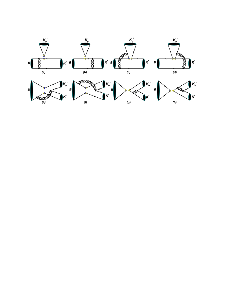
Figure 1: (Color online) Typical Feynman diagrams contributing to $B\to K_{0}^{*}K^{*}$ decays at leading order. In this figure, $B$ stands for $B_{u}$, $B_{d}$, and $B_{s}$, respectively. When we exchanged the position of $K_{0}^{*}$ and $K^{*}$, the other eight diagrams contribute to the considered decay modes will be easily obtained.

For the considered $B\to K_{0}^{*}K^{*}$ decays, the related weak effective Hamiltonian $H_{{\rm eff}}$ Buras96:weak can be written as

$$H_{\rm eff}\, = \,{G_{F}\over\sqrt{2}}\biggl{\{}V^{*}_{ub}V_{uq}[C_{1}(\mu)O_{1}^{u}(\mu)+C_{2}(\mu)O_{2}^{u}(\mu)]-V^{*}_{tb}V_{tq}[\sum_{i=3}^{10}C_{i}(\mu)O_{i}(\mu)]\biggr{\}}+{\rm H.c.}\;,$$ (16)

with $q=d$ or $s$, the Fermi constant $G_{F}=1.16639\times 10^{-5}{\rm GeV}^{-2}$, Cabibbo-Kobayashi-Maskawa(CKM) matrix elements $V$, and Wilson coefficients $C_{i}(\mu)$ at the renormalization scale $\mu$. The local four-quark operators $O_{i}(i=1,\cdots,10)$ are written as

1. (1) current-current(tree) operators

   $${\begin{array}[]{ll}\displaystyle O_{1}^{u}\,=\,(\bar{q}_{\alpha}u_{\beta})_{V-A}(\bar{u}_{\beta}b_{\alpha})_{V-A}\;,&\displaystyle O_{2}^{u}\,=\,(\bar{q}_{\alpha}u_{\alpha})_{V-A}(\bar{u}_{\beta}b_{\beta})_{V-A}\;;\end{array}}$$ (18)

2. (2) QCD penguin operators

   $${\begin{array}[]{ll}\displaystyle O_{3}\,=\,(\bar{q}_{\alpha}b_{\alpha})_{V-A}\sum_{q^{\prime}}(\bar{q}^{\prime}_{\beta}q^{\prime}_{\beta})_{V-A}\;,&\displaystyle O_{4}\,=\,(\bar{q}_{\alpha}b_{\beta})_{V-A}\sum_{q^{\prime}}(\bar{q}^{\prime}_{\beta}q^{\prime}_{\alpha})_{V-A}\;,\\ \displaystyle O_{5}\,=\,(\bar{q}_{\alpha}b_{\alpha})_{V-A}\sum_{q^{\prime}}(\bar{q}^{\prime}_{\beta}q^{\prime}_{\beta})_{V+A}\;,&\displaystyle O_{6}\,=\,(\bar{q}_{\alpha}b_{\beta})_{V-A}\sum_{q^{\prime}}(\bar{q}^{\prime}_{\beta}q^{\prime}_{\alpha})_{V+A}\;;\end{array}}$$ (21)

3. (3) electroweak penguin operators

   $${\begin{array}[]{ll}\displaystyle O_{7}\,=\,\frac{3}{2}(\bar{q}_{\alpha}b_{\alpha})_{V-A}\sum_{q^{\prime}}e_{q^{\prime}}(\bar{q}^{\prime}_{\beta}q^{\prime}_{\beta})_{V+A}\;,&\displaystyle O_{8}\,=\,\frac{3}{2}(\bar{q}_{\alpha}b_{\beta})_{V-A}\sum_{q^{\prime}}e_{q^{\prime}}(\bar{q}^{\prime}_{\beta}q^{\prime}_{\alpha})_{V+A}\;,\\ \displaystyle O_{9}\,=\,\frac{3}{2}(\bar{q}_{\alpha}b_{\alpha})_{V-A}\sum_{q^{\prime}}e_{q^{\prime}}(\bar{q}^{\prime}_{\beta}q^{\prime}_{\beta})_{V-A}\;,&\displaystyle O_{10}\,=\,\frac{3}{2}(\bar{q}_{\alpha}b_{\beta})_{V-A}\sum_{q^{\prime}}e_{q^{\prime}}(\bar{q}^{\prime}_{\beta}q^{\prime}_{\alpha})_{V-A}\;.\end{array}}$$ (24)

with the color indices $\alpha,\ \beta$ and the notations $(\bar{q}^{\prime}q^{\prime})_{V\pm A}=\bar{q}^{\prime}\gamma_{\mu}(1\pm\gamma_{5})q^{\prime}$. The index $q^{\prime}$ in the summation of the above operators runs through $u,\;d,\;s$, $c$, and $b$. The standard combinations $a_{i}$ of Wilson coefficients are defined as follows,

$$a_{1} = C_{2}+\frac{C_{1}}{3}\;,\qquad a_{2}=C_{1}+\frac{C_{2}}{3}\;,\quad a_{i}=C_{i}+\frac{C_{i\pm 1}}{3}(i=3-10)\;.$$ (25)

where the upper(lower) sign applies, when $i$ is odd(even).

Similar to $B\to K_{0}^{*}K$ decays Liu:scalar , there are eight types of diagrams contributing to $B\to K_{0}^{*}K^{*}$ modes at leading order, as illustrated in Fig. 1. They involve two classes of topologies with spectator and annihilation, respectively. Each kind of topology is classified into factorizable diagrams, in which hard gluon connects the quarks in the same meson, e.g., Fig. 1 (a) and 1 (b), and nonfactorizable diagrams, in which hard gluon attaches the quarks in two different mesons, e.g., Fig. 1 (c) and 1 (d). By calculating these Feynman diagrams, one can get the decay amplitudes of $B\to K_{0}^{*}K^{*}$ decays. Because the formulas of $B\to K_{0}^{*}K^{*}$ are similar to those of $B\to K_{0}^{*}K_{0}^{*}$ Liu:scalar , one can therefore obtain the expressions for all the diagrams just by replacing the corresponding wave functions and input parameters from $B\to K_{0}^{*}K_{0}^{*}$. So we do not present the detailed formulas in this paper.

By combining various of contributions from the relevant Feynman diagrams together, the total decay amplitudes for the considered $B\to K_{0}^{*}K^{*}$ decays can then read as,

1. The total decay amplitudes for charged $B_{u}$ decays:

   $${\cal A}(B_{u}\to K^{*+}{\overline{K}_{0}^{*}}^{0}) = \lambda_{u}\biggl{[}M_{nfa}C_{1}\biggr{]}-\lambda_{t}\biggl{[}F_{fs}(a_{4}-\frac{1}{2}a_{10})+F_{fs}^{P2}(a_{6}-\frac{1}{2}a_{8})$$ (26)

   $$+M_{nfs}(C_{3}-\frac{1}{2}C_{9})+M_{nfs}(C_{5}-\frac{1}{2}C_{7})+M_{nfa}$$

   $$\times(C_{3}+C_{9})+M_{nfa}^{P1}(C_{5}+C_{7})+f_{B}F_{fa}^{P2}(a_{6}+a_{8})\biggr{]}\;,$$

   where $\lambda_{u}=V_{ub}^{*}V_{ud}$ and $\lambda_{t}=V_{tb}^{*}V_{td}$. The decay amplitude of $B_{u}\to{K_{0}^{*}}^{+}\bar{K}^{*0}$ can be obtained directly from Eq. (26) with the replacement of $K^{*}\leftrightarrow{K_{0}^{*}}$, but without the contributions from the term $F_{fs}^{P2}$. The reason is that the emitted vector $K^{*}$ meson can not be produced via the scalar or pseudoscalar current.

2. The total decay amplitudes for neutral $B_{d}$ decays:

   $${\cal A}(B_{d}\to K^{*+}{K_{0}^{*}}^{-}) = \lambda_{u}\biggl{[}M_{nfa}C_{2}\biggr{]}-\lambda_{t}\biggl{[}M_{nfa}(C_{4}+C_{10})+M_{nfa}^{P2}(C_{6}+C_{8})$$ (27)

   $$+M_{nfa}[K^{*+}\leftrightarrow{K_{0}^{*}}^{-}](C_{4}-\frac{1}{2}C_{10})$$

   $$+M_{nfa}^{P2}[K^{*+}\leftrightarrow{K_{0}^{*}}^{-}](C_{6}-\frac{1}{2}C_{8})\biggr{]}\;,$$

   $${\cal A}(B_{d}\to K^{*0}{\overline{K}_{0}^{*}}^{0}) = -\lambda_{t}\biggl{[}F_{fs}(a_{4}-\frac{1}{2}a_{10})+F_{fs}^{P2}(a_{6}-\frac{1}{2}a_{8})+(M_{nfs}+M_{nfa})$$ (28)

   $$\times(C_{3}-\frac{1}{2}C_{9})+(M_{nfs}^{P1}+M_{nfa}^{P1})(C_{5}-\frac{1}{2}C_{7})+(M_{nfa}$$

   $$+[K^{*0}\leftrightarrow{\overline{K}_{0}^{*}}^{0}])(C_{4}-\frac{1}{2}C_{10})+(M_{nfa}^{P2}+[K^{*0}\leftrightarrow{\overline{K}_{0}^{*}}^{0}])$$

   $$\times(C_{6}-\frac{1}{2}C_{8})+f_{B}F_{fa}^{P2}(a_{6}-\frac{1}{2}a_{8})\biggr{]}\;.$$

   Similarly, the decay amplitudes of $B_{d}\to{K_{0}^{*}}^{+}K^{*-}$ and $B_{d}\to{K_{0}^{*}}^{0}\bar{K}^{*0}$ can also be obtained easily from Eqs. (27) and (28) with the replacements $K^{*}\leftrightarrow K_{0}^{*}$, respectively, and with the dropping of term $F_{sf}^{P2}$ for the latter mode.

3. The total decay amplitudes for $B_{s}$ decays:

   $${\cal A}(B_{s}\to{K_{0}^{*}}^{+}K^{*-}) = \lambda^{\prime}_{u}\biggl{[}F_{fs}a_{1}+M_{nfs}C_{1}+M_{nfa}C_{2}\biggr{]}-\lambda^{\prime}_{t}\biggl{[}F_{fs}(a_{4}+a_{10})$$ (29)

   $$+F_{fs}^{P2}(a_{6}+a_{8})+M_{nfs}(C_{3}+C_{9})+M_{nfs}^{P1}(C_{5}+C_{7})$$

   $$+M_{nfa}(C_{3}-\frac{1}{2}C_{9}+C_{4}-\frac{1}{2}C_{10})+M_{nfa}[{K_{0}^{*}}^{+}\leftrightarrow K^{*-}]$$

   $$\times(C_{4}+C_{10})+M_{nfa}^{P1}(C_{5}-\frac{1}{2}C_{7})+M_{nfa}^{P2}(C_{6}-\frac{1}{2}C_{8})$$

   $$+M_{nfa}^{P2}[{K_{0}^{*}}^{+}\leftrightarrow K^{*-}](C_{6}+C_{8})+f_{B_{s}}F_{fa}^{P2}(a_{6}-\frac{1}{2}a_{8})\biggr{]}\;,$$

   where $\lambda^{\prime}_{u}=V_{ub}^{*}V_{us}$ and $\lambda^{\prime}_{t}=V_{tb}^{*}V_{ts}$, and

   $${\cal A}(B_{s}\to{K_{0}^{*}}^{0}\bar{K}^{*0}) = -\lambda^{\prime}_{t}\biggl{[}F_{fs}(a_{4}-\frac{1}{2}a_{10})+F_{fs}^{P2}(a_{6}-\frac{1}{2}a_{8})+(M_{nfs}+M_{nfa})$$ (30)

   $$\times(C_{3}-\frac{1}{2}C_{9})+(M_{nfs}^{P1}+M_{nfa}^{P1})(C_{5}-\frac{1}{2}C_{7})+(M_{nfa}$$

   $$+[{K_{0}^{*}}^{0}\leftrightarrow\bar{K}^{*0}])(C_{4}-\frac{1}{2}C_{10})+(M_{nfa}^{P2}+[{K_{0}^{*}}^{0}\leftrightarrow\bar{K}^{*0}])$$

   $$\times(C_{6}-\frac{1}{2}C_{8})+f_{B_{s}}F_{fa}^{P2}(a_{6}-\frac{1}{2}a_{8})\biggr{]}\;.$$

There are other two $B_{s}$ decay channels, i.e., $B_{s}\to K^{*+}{K_{0}^{*}}^{-}$ and $B_{s}\to K^{*0}{\overline{K}_{0}^{*}}^{0}$, whose decay amplitudes can be derived from Eqs. (29) and (30) by the exchange of $K_{0}^{*}\leftrightarrow K^{*}$, respectively. Certainly, the $F_{fs}^{P2}$ term has no contribution to them either. Note that, based on the discussions of the factorizable annihilation contributions $F_{fa}$ in Ref. Liu:scalar , we here neglected this term in the above decay amplitudes for the considered $B\to K_{0}^{*}K^{*}$ decays analytically.

III Numerical Results and Discussions

In this section, we will present the theoretical predictions for the branching ratios and CP-violating asymmetries for those considered $B\to K_{0}^{*}K^{*}$ decay modes in the pQCD approach. In numerical calculations, central values of the input parameters will be used implicitly unless otherwise stated. The relevant QCD scale (GeV), masses (GeV), and $B$ meson lifetime(ps) are the following  Keum01:kpi ; Lu01:pipi ; Beringer12:pdg

$$\Lambda_{\overline{\mathrm{MS}}}^{(f=4)} = 0.250\;,\quad m_{W}=80.41\;,\quad m_{B}=5.28\;,\quad m_{B_{s}}=5.37\;,\quad m_{b}=4.8\;;$$

$$\tau_{B_{u}} = 1.641\;,\quad\tau_{B_{d}}=1.519\;,\quad\tau_{B_{s}}=1.497\;,\quad m_{K^{*}}=0.892\;,\quad m_{K_{0}^{*}(1430)}=1.425\;.$$ (31)

For the CKM matrix elements, we adopt the Wolfenstein parametrization and the updated parameters $A=0.811$, $\lambda=0.22535$, $\bar{\rho}=0.131^{+0.026}_{-0.013}$, and $\bar{\eta}=0.345^{+0.013}_{-0.014}$ Beringer12:pdg .

III.1 Branching Ratios

In this subsection, we will analyze the branching ratios of the considered $B\to K_{0}^{*}K^{*}$ decays in the pQCD approach. For $B\to K_{0}^{*}K^{*}$ decays, the decay rate can be written as

$$\Gamma=\frac{G_{F}^{2}m^{3}_{B}}{32\pi}(1-2r_{K_{0}^{*}}^{2})|{\cal A}(B\to K_{0}^{*}K^{*})|^{2}\;,$$ (32)

where the corresponding decay amplitudes ${\cal A}$ have been given explicitly in Eqs. (26-30). Using the decay amplitudes obtained in last section, it is straightforward to calculate the branching ratios with uncertainties as displayed in Table 1 - 3 for the considered decay modes. The major errors are induced by the uncertainties of the shape parameters $\omega_{b}=0.40\pm 0.04$ GeV for $B_{u,d}$ decays, $\omega_{B_{s}}=0.50\pm 0.05$ GeV for $B_{s}$ decays, the scalar decay constant $\bar{f}_{K_{0}^{*}}$ of $K_{0}^{*}$ meson, the decay constants $f_{K^{*}}^{(T)}$ of vector $K^{*}$ meson, the Gegenbauer moments $B_{i}(i=1,3)$ for the scalar $K_{0}^{*}$, the Gegenbauer moments $a_{i}(i=1,2)$ for the vector $K^{*}$ meson, and CKM matrix elements $V_{i}$ ($\bar{\rho},\bar{\eta}$), respectively.

Table 1: The pQCD predictions for the branching ratios of $B_{u}\to{K_{0}^{*}}^{+}\overline{K}^{*0}$ and $K^{*+}{\overline{K}_{0}^{*}}^{0}$ decays in different scenarios: the first (second) entry corresponds to S1(S2).

Decay modes	Branching ratios
$B_{u}\to{K_{0}^{*}}^{+}\overline{K}^{*0}$	$\begin{array}[]{l}2.1^{+1.5}_{-0.9}(\omega_{b})^{+0.4}_{-0.4}(\bar{f}_{K_{0}^{*}})^{+0.3}_{-0.3}(f^{(T)}_{K^{*}})^{+0.1}_{-0.2}(B_{i})^{+0.2}_{-0.1}(a_{i})^{+0.1}_{-0.2}(V_{i})^{+0.4}_{-0.2}(a_{t})\times 10^{-7}\\ 1.3^{+0.5}_{-0.3}(\omega_{b})^{+0.3}_{-0.3}(\bar{f}_{K_{0}^{*}})^{+0.1}_{-0.1}(f^{(T)}_{K^{*}})^{+0.1}_{-0.1}(B_{i})^{+0.1}_{-0.1}(a_{i})^{+0.0}_{-0.1}(V_{i})^{+0.4}_{-0.2}(a_{t})\times 10^{-6}\end{array}$
$B_{u}\to K^{*+}{\overline{K}_{0}^{*}}^{0}$	$\begin{array}[]{l}6.0^{+1.4}_{-1.0}(\omega_{b})^{+1.3}_{-1.2}(\bar{f}_{K_{0}^{*}})^{+0.3}_{-0.3}(f^{(T)}_{K^{*}})^{+0.4}_{-0.3}(B_{i})^{+0.1}_{-0.1}(a_{i})^{+0.5}_{-0.5}(V_{i})^{+0.8}_{-0.5}(a_{t})\times 10^{-7}\\ 1.5^{+0.5}_{-0.3}(\omega_{b})^{+0.4}_{-0.3}(\bar{f}_{K_{0}^{*}})^{+0.1}_{-0.1}(f^{(T)}_{K^{*}})^{+0.3}_{-0.1}(B_{i})^{+0.2}_{-0.1}(a_{i})^{+0.1}_{-0.1}(V_{i})^{+0.5}_{-0.3}(a_{t})\times 10^{-6}\end{array}$

Table 2: Same as Table 1 but for neutral $B_{d}\to K_{0}^{*}K^{*}$ decays in both scenarios.

Decay modes	Branching ratios
$B_{d}\to{K_{0}^{*}}^{0}\overline{K}^{*0}+K^{*0}{\overline{K}_{0}^{*}}^{0}$	$\begin{array}[]{l}6.4^{+0.5}_{-0.6}(\omega_{b})^{+1.3}_{-1.2}(\bar{f}_{K_{0}^{*}})^{+0.7}_{-0.7}(f^{(T)}_{K^{*}})^{+1.6}_{-1.5}(B_{i})^{+0.8}_{-0.8}(a_{i})^{+0.2}_{-0.3}(V_{i})^{+0.2}_{-0.5}(a_{t})\times 10^{-7}\\ 5.9^{+0.7}_{-0.6}(\omega_{b})^{+1.4}_{-1.2}(\bar{f}_{K_{0}^{*}})^{+0.6}_{-0.4}(f^{(T)}_{K^{*}})^{+5.9}_{-3.2}(B_{i})^{+0.5}_{-0.4}(a_{i})^{+0.2}_{-0.3}(V_{i})^{+0.7}_{-0.6}(a_{t})\times 10^{-7}\end{array}$
$B_{d}/\bar{B}_{d}\to{K_{0}^{*}}^{0}\overline{K}^{*0}(K^{*0}{\overline{K}_{0}^{*}}^{0})$	$\begin{array}[]{l}5.0^{+2.2}_{-1.3}(\omega_{b})^{+1.1}_{-1.0}(\bar{f}_{K_{0}^{*}})^{+0.6}_{-0.6}(f^{(T)}_{K^{*}})^{+0.4}_{-0.3}(B_{i})^{+0.2}_{-0.1}(a_{i})^{+0.1}_{-0.3}(V_{i})^{+0.5}_{-0.5}(a_{t})\times 10^{-7}\\ 2.3^{+0.8}_{-0.5}(\omega_{b})^{+0.5}_{-0.5}(\bar{f}_{K_{0}^{*}})^{+0.1}_{-0.1}(f^{(T)}_{K^{*}})^{+0.4}_{-0.2}(B_{i})^{+0.2}_{-0.2}(a_{i})^{+0.0}_{-0.1}(V_{i})^{+0.7}_{-0.5}(a_{t})\times 10^{-6}\end{array}$
Decay modes	Branching ratios ($10^{-6}$)
$B_{d}\to{K_{0}^{*}}^{+}K^{*-}+K^{*+}{K_{0}^{*}}^{-}$	$\begin{array}[]{l}2.8^{+0.2}_{-0.3}(\omega_{b})^{+0.6}_{-0.6}(\bar{f}_{K_{0}^{*}})^{+0.1}_{-0.2}(f^{(T)}_{K^{*}})^{+0.4}_{-0.4}(B_{i})^{+0.1}_{-0.0}(a_{i})^{+0.1}_{-0.2}(V_{i})^{+0.0}_{-0.1}(a_{t})\\ 1.1^{+0.1}_{-0.1}(\omega_{b})^{+0.2}_{-0.3}(\bar{f}_{K_{0}^{*}})^{+0.0}_{-0.1}(f^{(T)}_{K^{*}})^{+1.1}_{-0.6}(B_{i})^{+0.1}_{-0.1}(a_{i})^{+0.0}_{-0.1}(V_{i})^{+0.0}_{-0.1}(a_{t})\end{array}$
$B_{d}/\bar{B}_{d}\to{K_{0}^{*}}^{+}K^{*-}$	$\begin{array}[]{l}4.5^{+0.4}_{-0.4}(\omega_{b})^{+0.9}_{-0.9}(\bar{f}_{K_{0}^{*}})^{+0.2}_{-0.2}(f^{(T)}_{K^{*}})^{+0.6}_{-0.6}(B_{i})^{+0.3}_{-0.3}(a_{i})^{+0.2}_{-0.3}(V_{i})^{+0.1}_{-0.1}(a_{t})\\ 2.9^{+0.3}_{-0.4}(\omega_{b})^{+0.6}_{-0.7}(\bar{f}_{K_{0}^{*}})^{+0.2}_{-0.1}(f^{(T)}_{K^{*}})^{+2.0}_{-1.4}(B_{i})^{+0.1}_{-0.1}(a_{i})^{+0.2}_{-0.2}(V_{i})^{+0.1}_{-0.2}(a_{t})\end{array}$
$B_{d}/\bar{B}_{d}\to K^{*+}{K_{0}^{*}}^{-}$	$\begin{array}[]{l}1.7^{+0.2}_{-0.2}(\omega_{b})^{+0.3}_{-0.3}(\bar{f}_{K_{0}^{*}})^{+0.1}_{-0.1}(f^{(T)}_{K^{*}})^{+0.2}_{-0.2}(B_{i})^{+0.1}_{-0.1}(a_{i})^{+0.1}_{-0.2}(V_{i})^{+0.1}_{-0.1}(a_{t})\\ 1.1^{+0.1}_{-0.2}(\omega_{b})^{+0.2}_{-0.3}(\bar{f}_{K_{0}^{*}})^{+0.1}_{-0.0}(f^{(T)}_{K^{*}})^{+0.6}_{-0.5}(B_{i})^{+0.0}_{-0.1}(a_{i})^{+0.1}_{-0.1}(V_{i})^{+0.0}_{-0.1}(a_{t})\end{array}$

Table 3: Same as Table 1 but for strange $B_{s}\to K_{0}^{*}K^{*}$ decays in both scenarios.

Decay modes	Branching ratios ($10^{-5}$)
$B_{s}\to{K_{0}^{*}}^{0}\overline{K}^{*0}+K^{*0}{\overline{K}_{0}^{*}}^{0}$	$\begin{array}[]{l}1.3^{+0.2}_{-0.1}(\omega_{bs})^{+0.3}_{-0.2}(\bar{f}_{K_{0}^{*}})^{+0.2}_{-0.1}(f^{(T)}_{K^{*}})^{+0.4}_{-0.3}(B_{i})^{+0.2}_{-0.1}(a_{i})^{+0.0}_{-0.0}(V_{i})^{+0.1}_{-0.1}(a_{t})\\ 1.3^{+0.2}_{-0.2}(\omega_{bs})^{+0.3}_{-0.3}(\bar{f}_{K_{0}^{*}})^{+0.1}_{-0.1}(f^{(T)}_{K^{*}})^{+1.2}_{-0.7}(B_{i})^{+0.1}_{-0.1}(a_{i})^{+0.0}_{-0.0}(V_{i})^{+0.1}_{-0.2}(a_{t})\end{array}$
$B_{s}/\bar{B}_{s}\to{K_{0}^{*}}^{0}\overline{K}^{*0}(K^{*0}{\overline{K}_{0}^{*}}^{0})$	$\begin{array}[]{l}0.9^{+0.3}_{-0.2}(\omega_{bs})^{+0.2}_{-0.2}(\bar{f}_{K_{0}^{*}})^{+0.1}_{-0.1}(f^{(T)}_{K^{*}})^{+0.1}_{-0.1}(B_{i})^{+0.1}_{-0.1}(a_{i})^{+0.0}_{-0.0}(V_{i})^{+0.1}_{-0.1}(a_{t})\\ 5.4^{+1.5}_{-0.9}(\omega_{bs})^{+1.3}_{-1.1}(\bar{f}_{K_{0}^{*}})^{+0.2}_{-0.2}(f^{(T)}_{K^{*}})^{+0.9}_{-0.5}(B_{i})^{+0.9}_{-0.6}(a_{i})^{+0.0}_{-0.0}(V_{i})^{+1.7}_{-1.1}(a_{t})\end{array}$
Decay modes	Branching ratios ($10^{-5}$)
$B_{s}\to{K_{0}^{*}}^{+}K^{*-}+K^{*+}{K_{0}^{*}}^{-}$	$\begin{array}[]{l}1.3^{+0.2}_{-0.1}(\omega_{bs})^{+0.3}_{-0.2}(\bar{f}_{K_{0}^{*}})^{+0.1}_{-0.1}(f^{(T)}_{K^{*}})^{+0.4}_{-0.2}(B_{i})^{+0.1}_{-0.1}(a_{i})^{+0.1}_{-0.0}(V_{i})^{+0.1}_{-0.1}(a_{t})\\ 1.5^{+0.4}_{-0.3}(\omega_{bs})^{+0.4}_{-0.3}(\bar{f}_{K_{0}^{*}})^{+0.1}_{-0.0}(f^{(T)}_{K^{*}})^{+1.0}_{-0.4}(B_{i})^{+0.1}_{-0.0}(a_{i})^{+0.1}_{-0.0}(V_{i})^{+0.3}_{-0.2}(a_{t})\end{array}$
$B_{s}/\bar{B}_{s}\to{K_{0}^{*}}^{+}K^{*-}$	$\begin{array}[]{l}0.9^{+0.3}_{-0.1}(\omega_{bs})^{+0.2}_{-0.2}(\bar{f}_{K_{0}^{*}})^{+0.1}_{-0.1}(f^{(T)}_{K^{*}})^{+0.2}_{-0.1}(B_{i})^{+0.0}_{-0.0}(a_{i})^{+0.0}_{-0.0}(V_{i})^{+0.1}_{+0.1}(a_{t})\\ 4.0^{+1.3}_{-0.7}(\omega_{bs})^{+1.0}_{-0.8}(\bar{f}_{K_{0}^{*}})^{+0.2}_{-0.1}(f^{(T)}_{K^{*}})^{+0.8}_{-0.3}(B_{i})^{+0.6}_{-0.4}(a_{i})^{+0.1}_{-0.1}(V_{i})^{+1.4}_{-0.8}(a_{t})\end{array}$
$B_{s}/\bar{B}_{s}\to K^{*+}{K_{0}^{*}}^{-}$	$\begin{array}[]{l}0.9^{+0.2}_{-0.1}(\omega_{bs})^{+0.2}_{-0.2}(\bar{f}_{K_{0}^{*}})^{+0.1}_{-0.1}(f^{(T)}_{K^{*}})^{+0.1}_{-0.1}(B_{i})^{+0.2}_{-0.1}(a_{i})^{+0.0}_{-0.0}(V_{i})^{+0.2}_{-0.1}(a_{t})\\ 6.1^{+1.5}_{-0.9}(\omega_{bs})^{+1.4}_{-1.3}(\bar{f}_{K_{0}^{*}})^{+0.3}_{-0.2}(f^{(T)}_{K^{*}})^{+1.0}_{-0.6}(B_{i})^{+1.1}_{-0.9}(a_{i})^{+0.1}_{-0.1}(V_{i})^{+1.9}_{-1.2}(a_{t})\end{array}$

Based on the above numerical results of the branching ratios given at leading order in the pQCD approach for the considered decay modes, some remarks are as follows:

1. Generally speaking, the theoretical predictions for the considered decays in the pQCD approach have relatively large errors arising from the still large uncertainties of many input parameters. Furthermore, the numerical results for the branching ratios suffer more from the errors induced by the less constrained hadronic parameters of the light scalar $K_{0}^{*}$, such as the scalar decay constant $\bar{f}_{K_{0}^{*}}$ and the Gegenbauer coefficients $B_{i}(i=1,3)$. Additionally, in this work, as displayed in the above tables, the higher order contributions are also simply investigated by exploring the variation of the hard scale $t_{\rm max}$, i.e., from $0.8t$ to $1.2t$ (not changing $1/b_{i},i=1,2,3$), in the hard kernel, which have been counted into one of the source of theoretical uncertainties.

2. The pQCD predictions for the CP-averaged $Br(B_{u}\to{K_{0}^{*}}^{+}\overline{K}^{*0})$ and $Br(B_{u}\to K^{*+}{\overline{K}_{0}^{*}}^{0})$ are in the order of $10^{-6}$ in S2, which are lager than those in S1, and can be tested by the future $B$ physics experiments. Moreover, one can define the ratios of the branching ratios of the same decay mode but in different scenarios as the following,

   $$\frac{Br(B_{u}\to{K_{0}^{*}}^{+}\overline{K}^{*0})_{\rm S2}}{Br(B_{u}\to{K_{0}^{*}}^{+}\overline{K}^{*0})_{\rm S1}} = 6.2\;,\qquad\frac{Br(B_{u}\to K^{*+}{\overline{K}_{0}^{*}}^{0})_{\rm S2}}{Br(B_{u}\to K^{*+}{\overline{K}_{0}^{*}}^{0})_{\rm S1}}=2.5\;;$$ (33)

   where the central values are quoted for clarification. The above two patterns imply the different QCD dynamics involved in the corresponding decay channels, which can be tested with the future precision measurements.

3. For the neutral $B_{d}$ decays, which include the pure penguin contribution modes, i.e., $B_{d}\to K^{*0}{\overline{K}_{0}^{*}}^{0}$ and $B_{d}\to{K_{0}^{*}}^{0}\overline{K}^{*0}$, and the pure annihilation contribution channels, i.e., $B_{d}\to K^{*+}{K_{0}^{*}}^{-}$ and $B_{d}\to{K_{0}^{*}}^{+}K^{*-}$, respectively. The analysis for these four decay modes are a little complicated, which is just because both $B_{d}$ and $\bar{B}_{d}$ can decay into the same final states simultaneously, in other words, the final states in the considered $B_{d}$ decays are not the CP-eigensates. Due to the $B_{d}-\bar{B}_{d}$ mixing, it is very difficult for us to distinguish the $B_{d}$ from the $\bar{B}_{d}$. However, fortunately, it is easy to identify the final states in the considered decays. We therefore sum up $B_{d}/\bar{B}_{d}\to K^{*0}{\overline{K}_{0}^{*}}^{0}$ as one channel, and $B_{d}/\bar{B}_{d}\to{K_{0}^{*}}^{0}\overline{K}^{*0}$ as another. Similarly, we will have $B_{d}/\bar{B}_{d}\to K^{*+}{K_{0}^{*}}^{-}$ as one mode, and $B_{d}/\bar{B}_{d}\to{K_{0}^{*}}^{+}K^{*-}$ as another. Moreover, following the convention by the experimental measurements Beringer12:pdg ; Amhis12:hfag , we also define the averaged quantity of the two channels, i.e., $B_{d}\to K^{*0}{\overline{K}_{0}^{*}}^{0}+{K_{0}^{*}}^{0}\overline{K}^{*0}$ and $B_{d}\to K^{*+}{K_{0}^{*}}^{-}+{K_{0}^{*}}^{+}K^{*-}$. The same phenomena will also occur in the decays of the $B_{s}$ meson.

4. The theoretical predictions on the branching ratios of the $B_{d}$ meson decays in the pQCD approach have been presented in Table 2. For the pure penguin $B_{d}/\bar{B}_{d}\to{K_{0}^{*}}^{0}\overline{K}^{*0}$, $B_{d}/\bar{B}_{d}\to K^{*0}{\overline{K}_{0}^{*}}^{0}$, and $B_{d}\to{K_{0}^{*}}^{0}\overline{K}^{*0}+K^{*0}{\overline{K}_{0}^{*}}^{0}$ channels, the pQCD predictions for the former two decays show that the branching ratios (about $2\times 10^{-6}$) in S2 are larger than that (about $5\times 10^{-7}$) in S1, which results in the ratio $Br(B_{d}/\bar{B}_{d}\to{K_{0}^{*}}^{0}\overline{K}^{*0}(K^{*0}{\overline{K}_{0}^{*}}^{0}))_{\rm S2}/Br(B_{d}/\bar{B}_{d}\to{K_{0}^{*}}^{0}\overline{K}^{*0}(K^{*0}{\overline{K}_{0}^{*}}^{0}))_{\rm S1}\approx 4.6$; while the pQCD predictions for the latter one in both scenarios are similar, which leads to the ratio $Br(B_{d}\to K^{*0}{\overline{K}_{0}^{*}}^{0}+{K_{0}^{*}}^{0}\overline{K}^{*0})_{\rm S1}/Br(B_{d}\to K^{*0}{\overline{K}_{0}^{*}}^{0}+{K_{0}^{*}}^{0}\overline{K}^{*0})_{\rm S2}\approx 1.1$. Note that due to the charge conjugation between the pure penguin channels $B_{d}\to{K_{0}^{*}}^{0}\overline{K}^{*0}$ and $\bar{B}_{d}\to{\overline{K}_{0}^{*}}^{0}K^{*0}$ and the domination of the real contributions arising from the factorizable emission diagrams, e.g., Fig. 1 (a) and (b), in the considered channels, which give the same branching ratios for $B_{d}/\bar{B}_{d}\to{K_{0}^{*}}^{0}\overline{K}^{*0}$ and $B_{d}/\bar{B}_{d}\to{\overline{K}_{0}^{*}}^{0}K^{*0}$ modes, as presented in Table 2. Certainly, the similar phenomena will also appear in the related $B_{s}$ meson decays.

   As shown in Eq. (1), only a preliminary upper limit for $B^{0}\to{K_{0}^{*}(1430)}^{0}\overline{K}^{*0}$ decay is available now. By comparison, one can easily find from Table 2 that the pQCD predictions in both scenarios are all consistent with this upper limit. The branching ratios in the order of $10^{-6}$ and above are expected to be tested in the near future $B$ meson experiments.

5. For the pure annihilation $B_{d}/\bar{B}_{d}\to{K_{0}^{*}}^{+}K^{*-}$, $B_{d}/\bar{B}_{d}\to K^{*+}{K_{0}^{*}}^{-}$, and $B_{d}\to{K_{0}^{*}}^{+}K^{*-}+K^{*+}{K_{0}^{*}}^{-}$ channels, as listed in Table 2, the pQCD predictions for the branching ratios in both scenarios are in order of $10^{-6}$. Furthermore, one can find that the numerical pQCD results for the branching ratios in S1 are clearly larger than those in S2, which are rather different from the situation of $B_{d}\to{K_{0}^{*}}^{0}\overline{K}^{*0}$ and $K^{*0}{\overline{K}_{0}^{*}}^{0}$ decays. Although the charge conjugation also exists in the channels $B_{d}\to K^{*+}{K_{0}^{*}}^{-}$ and $\bar{B}_{d}\to K^{*-}{K_{0}^{*}}^{+}$, the interference between tree and penguin topologies makes the decay amplitudes for the considered modes different from those for the $B_{d}$ meson decaying into two neutral final states, which therefore give different branching ratios for $B_{d}/\bar{B}_{d}\to{K_{0}^{*}}^{+}K^{*-}$ and $B_{d}/\bar{B}_{d}\to K^{*+}{K_{0}^{*}}^{-}$ as exhibited in Table 2.

   Additionally, one can define the interesting ratios among the same decay modes but in different scenarios,

   $$\frac{Br(B_{d}\to{K_{0}^{*}}^{+}K^{*-}+K^{*+}{K_{0}^{*}}^{-})_{\rm S1}}{Br(B_{d}\to{K_{0}^{*}}^{+}K^{*-}+K^{*+}{K_{0}^{*}}^{-})_{\rm S2}} = 2.5\;,$$ (34)

   $$\frac{Br(B_{d}/\bar{B}_{d}\to{K_{0}^{*}}^{+}K^{*-})_{\rm S1}}{Br(B_{d}/\bar{B}_{d}\to{K_{0}^{*}}^{+}K^{*-})_{\rm S2}} = 1.6\;,\qquad\frac{Br(B_{d}/\bar{B}_{d}\to K^{*+}{K_{0}^{*}}^{-})_{\rm S1}}{Br(B_{d}/\bar{B}_{d}\to K^{*+}{K_{0}^{*}}^{-})_{\rm S2}}=1.5\;,$$ (35)

   where only the central values of the branching ratios are considered for clarification.

   Very recently, LHCb Powell11:LHCb and CDF Ruffini11:CDF Collaborations have measured the pure annihilation modes of charmless hadronic $B$ meson decays, such as $B_{d}\to K^{+}K^{-}$ and $B_{s}\to\pi^{+}\pi^{-}$, respectively. It is therefore believed that such large decay rates (about $(1\sim 5)\times 10^{-6}$) for the considered pure annihilation decays in this paper could be tested by the ongoing LHC experiments and/or the forthcoming Super-$B$ factory in the near future. If the numerical results of the pure annihilation decays can be confirmed by the future measurements at the predicted level, on one hand, which will provide much more evidences to support the successful pQCD approach in calculating the annihilation diagrams; on the other hand, which will provide more important information on the sizable annihilation contributions in heavy $B$ meson physics and further shed light on the underlying mechanism of the annihilated $B$ meson decays.

6. For the considered $B_{s}$ meson decays, all the predicted branching ratios are in the range of $(1\sim 6)\times 10^{-5}$, which can be seen in Table 3 and will be tested by the LHC experiments. In terms of the channels with the neutral final states, which are the pure penguin induced decays, the branching ratios for the averaged channel $B_{s}\to{K_{0}^{*}}^{0}\overline{K}^{*0}+K^{*0}{\overline{K}_{0}^{*}}^{0}$ are equal to each other in two scenarios. The branching ratios for the two summed channels, $B_{s}/\bar{B}_{s}\to{K_{0}^{*}}^{0}\overline{K}^{*0}$ and $B_{s}/\bar{B}_{s}\to K^{*0}{\overline{K}_{0}^{*}}^{0}$ in S2, however, are larger than those in S1 with a factor about six.

   The pQCD predictions for the branching ratios for the averaged channel $B_{s}\to{K_{0}^{*}}^{+}K^{*-}+K^{*+}{K_{0}^{*}}^{-}$ are similar in size in both scenarios. Analogous to the decays with the neutral final states, the pQCD results for $B_{s}/\bar{B}_{s}\to{K_{0}^{*}}^{+}K^{*-}$ and $B_{s}/\bar{B}_{s}\to K^{*+}{K_{0}^{*}}^{-}$ in S2 are larger than those in S1 with a factor about 4 and 6, respectively. These results are expected to be examined by the measurements in the future.

7. For the considered pure penguin decays, $B_{d/s}\to{K_{0}^{*}}^{0}\overline{K}^{*0}$ and $K^{*0}{\overline{K}_{0}^{*}}^{0}$, we get the ratios in two scenarios between the branching ratios of $B_{d}$ and $B_{s}$ decays in the pQCD approach,

   $$\frac{\tau_{B_{d}}}{\tau_{B_{s}}}\cdot\frac{Br(B_{s}\to{K_{0}^{*}}^{0}\overline{K}^{*0}+K^{*0}{\overline{K}_{0}^{*}}^{0})}{Br(B_{d}\to{K_{0}^{*}}^{0}\overline{K}^{*0}+K^{*0}{\overline{K}_{0}^{*}}^{0})} = 20.6\;,\qquad\frac{\tau_{B_{d}}}{\tau_{B_{s}}}\cdot\frac{Br(B_{s}/\bar{B}_{s}\to{K_{0}^{*}}^{0}\overline{K}^{*0}(K^{*0}{\overline{K}_{0}^{*}}^{0}))}{Br(B_{d}/\bar{B}_{d}\to{K_{0}^{*}}^{0}\overline{K}^{*0}(K^{*0}{\overline{K}_{0}^{*}}^{0}))}=18.3\;;$$ (36)

   in S1, and

   $$\frac{\tau_{B_{d}}}{\tau_{B_{s}}}\cdot\frac{Br(B_{s}\to{K_{0}^{*}}^{0}\overline{K}^{*0}+K^{*0}{\overline{K}_{0}^{*}}^{0})}{Br(B_{d}\to{K_{0}^{*}}^{0}\overline{K}^{*0}+K^{*0}{\overline{K}_{0}^{*}}^{0})} = 22.4\;,\qquad\frac{\tau_{B_{d}}}{\tau_{B_{s}}}\cdot\frac{Br(B_{s}/\bar{B}_{s}\to{K_{0}^{*}}^{0}\overline{K}^{*0}(K^{*0}{\overline{K}_{0}^{*}}^{0}))}{Br(B_{d}/\bar{B}_{d}\to{K_{0}^{*}}^{0}\overline{K}^{*0}(K^{*0}{\overline{K}_{0}^{*}}^{0}))}=23.8\;;$$ (37)

   in S2, in which the central values of the branching ratios are quoted. From the analytical expressions for the decay amplitudes of these $B_{d}$ and $B_{s}$ modes, e.g., Eqs. (28) and (30), one can easily find that the main difference is just from the involved CKM factors $\lambda_{t}$ and $\lambda^{\prime}_{t}$ with $|\lambda^{\prime}_{t}/\lambda_{t}|^{2}=22.5$.

8. Frankly speaking, the measurements at the experimental aspect are not yet available up to now. We therefore can not make any judgements on whether the scenario 1 or scenario 2 of the scalar $K_{0}^{*}$ is favored by the considered decays. The pQCD predictions for the branching ratios of the considered $B\to K_{0}^{*}K^{*}$ decays will be tested by the LHC experiments and/or forthcoming Super-$B$ facility.

Here, based on the numerical calculations of the branching ratios, we also examine the effects coming from the annihilation diagrams. In those considered $B\to K_{0}^{*}K^{*}$ decays, when the annihilation contributions are not taken into account, the relevant predictions on the branching ratios in the pQCD approach are as follows:

$$Br(B_{u}\to{K_{0}^{*}}^{+}\overline{K}^{*0}) = 7.8\times 10^{-7},\qquad Br(B_{u}\to K^{*+}{\overline{K}_{0}^{*}}^{0})=6.1\times 10^{-7}\;,$$ (38)

$$Br(B_{d}\to{K_{0}^{*}}^{0}\overline{K}^{*0}+K^{*0}{\overline{K}_{0}^{*}}^{0}) = 1.7\times 10^{-8},\quad Br(B_{d}/\bar{B}_{d}\to{K_{0}^{*}}^{0}\overline{K}^{*0}(K^{*0}{\overline{K}_{0}^{*}}^{0}))=1.3\times 10^{-6}\;,$$ (39)

$$Br(B_{s}\to{K_{0}^{*}}^{0}\overline{K}^{*0}+K^{*0}{\overline{K}_{0}^{*}}^{0}) = 3.2\times 10^{-7},\quad Br(B_{s}/\bar{B}_{s}\to{K_{0}^{*}}^{0}\overline{K}^{*0}(K^{*0}{\overline{K}_{0}^{*}}^{0}))=2.4\times 10^{-5}\;,$$ (40)

$$Br(B_{s}\to{K_{0}^{*}}^{+}K^{*-}+K^{*+}{K_{0}^{*}}^{-}) = 0.3\times 10^{-5},$$ (41)

$$Br(B_{s}/\bar{B}_{s}\to{K_{0}^{*}}^{+}K^{*-}) = 2.2\times 10^{-5},\quad Br(B_{s}/\bar{B}_{s}\to K^{*+}{K_{0}^{*}}^{-})=2.1\times 10^{-5}\;;$$ (42)

in scenario 1, and

$$Br(B_{u}\to{K_{0}^{*}}^{+}\overline{K}^{*0}) = 1.8\times 10^{-6},\qquad Br(B_{u}\to K^{*+}{\overline{K}_{0}^{*}}^{0})=1.5\times 10^{-6}\;,$$ (43)

$$Br(B_{d}\to{K_{0}^{*}}^{0}\overline{K}^{*0}+K^{*0}{\overline{K}_{0}^{*}}^{0}) = 3.4\times 10^{-8},\quad Br(B_{d}/\bar{B}_{d}\to{K_{0}^{*}}^{0}\overline{K}^{*0}(K^{*0}{\overline{K}_{0}^{*}}^{0}))=3.0\times 10^{-6}\;,$$ (44)

$$Br(B_{s}\to{K_{0}^{*}}^{0}\overline{K}^{*0}+K^{*0}{\overline{K}_{0}^{*}}^{0}) = 3.0\times 10^{-7},\quad Br(B_{s}/\bar{B}_{s}\to{K_{0}^{*}}^{0}\overline{K}^{*0}(K^{*0}{\overline{K}_{0}^{*}}^{0}))=5.4\times 10^{-5}\;,$$ (45)

$$Br(B_{s}\to{K_{0}^{*}}^{+}K^{*-}+K^{*+}{K_{0}^{*}}^{-}) = 0.7\times 10^{-5},$$ (46)

$$Br(B_{s}/\bar{B}_{s}\to{K_{0}^{*}}^{+}K^{*-}) = 5.0\times 10^{-5},\quad Br(B_{s}/\bar{B}_{s}\to K^{*+}{K_{0}^{*}}^{-})=4.9\times 10^{-5}\;.$$ (47)

in scenario 2, in which only the central values are considered for estimating the contributions arising from the annihilation diagrams in various decay channels. By comparison, one can easily find the following points:

• For the charged $B_{u}$ decays, the weak annihilation contributions play more important roles in the $B_{u}\to{K_{0}^{*}}^{+}\overline{K}^{*0}$ than that in the $B_{u}\to K^{*+}{\overline{K}_{0}^{*}}^{0}$.

• For the pure penguin $B_{d}$ and $B_{s}$ decays, apart from the $B_{s}/\bar{B}_{s}\to{K_{0}^{*}}^{0}\overline{K}^{*0}(K^{*0}{\overline{K}_{0}^{*}}^{0})$ in S2, other channels are basically dominated by the weak annihilation contributions, particularly, for $B_{d/s}\to{K_{0}^{*}}^{0}\overline{K}^{*0}+K^{*0}{\overline{K}_{0}^{*}}^{0}$ modes.

• For other $B_{s}$ decays, the significant contributions given by the weak annihilation diagrams can also be clearly observed. Of course, the reliability of the contributions from the annihilation diagrams to these considered decays calculated in the pQCD approach will be examined by the relevant experiments in the future.

III.2 CP-violating Asymmetries

Now we turn to the evaluations of the CP-violating asymmetries of $B\to K_{0}^{*}K^{*}$ decays in the pQCD approach. For the charged $B_{u}$ meson decays, the direct CP violation $A_{CP}^{\rm dir}$ can be defined as,

$$A_{CP}^{\rm dir}=\frac{|\overline{\cal A}_{f}|^{2}-|{\cal A}_{f}|^{2}}{|\overline{\cal A}_{f}|^{2}+|{\cal A}_{f}|^{2}},$$ (48)

where ${\cal A}_{f}$ stands for the decay amplitude of $B_{u}\to{K_{0}^{*}}^{+}\overline{K}^{*0}$ and $B_{u}\to K^{*+}{\overline{K}_{0}^{*}}^{0}$, respectively, while $\overline{{\cal A}}_{f}$ denotes the charge conjugation one correspondingly. Using Eq. (48), we find the following pQCD predictions (in unit of $10^{-2}$):

$$A_{CP}^{\rm dir}(B_{u}\to{K_{0}^{*}}^{+}\overline{K}^{*0}) = \left\{\begin{array}[]{ll}-32.6^{+10.5}_{-11.3}(\omega_{b})^{+0.7}_{-0.8}(\bar{f}_{K_{0}^{*}})^{+3.1}_{-4.0}(f_{K^{*}})^{+3.6}_{-4.8}(B_{i})^{+5.4}_{-1.7}(a_{i})^{+1.1}_{-2.4}(V_{i})^{+2.1}_{-3.9}(a_{t})&\hskip 2.84544pt({\rm S1})\\ -34.9^{+5.0}_{-4.5}(\omega_{b})^{+0.5}_{-0.4}(\bar{f}_{K_{0}^{*}})^{+1.6}_{-1.5}(f_{K^{*}})^{+6.9}_{-9.0}(B_{i})^{+1.5}_{-1.6}(a_{i})^{+1.4}_{-2.2}(V_{i})^{+1.6}_{-0.2}(a_{t})&\hskip 2.84544pt({\rm S2})\\ \end{array}\right.\;,$$ (51)

$$A_{CP}^{\rm dir}(B_{u}\to{K}^{*+}{\overline{K}_{0}^{*}}^{0}) = \left\{\begin{array}[]{ll}\hskip 7.39755pt43.6^{+3.7}_{-2.2}(\omega_{b})^{+1.1}_{-1.3}(\bar{f}_{K_{0}^{*}})^{+2.0}_{-1.7}(f_{K^{*}})^{+13.0}_{-13.7}(B_{i})^{+2.8}_{-2.6}(a_{i})^{+1.7}_{-1.6}(V_{i})^{+2.0}_{-2.7}(a_{t})&\hskip 2.84544pt({\rm S1})\\ -67.9^{+4.9}_{-5.2}(\omega_{b})^{+0.8}_{-1.0}(\bar{f}_{K_{0}^{*}})^{+1.7}_{-1.6}(f_{K^{*}})^{+16.0}_{-14.9}(B_{i})^{+1.2}_{-0.6}(a_{i})^{+1.9}_{-3.8}(V_{i})^{+3.3}_{-1.3}(a_{t})&\hskip 2.84544pt({\rm S2})\\ \end{array}\right.\;;$$ (54)

Note that these two channels exhibit large direct CP-violating asymmetries in both scenarios in the pQCD approach, which indicates that the contribution of the penguin diagrams is sizable. Combining the large CP-averaged branching ratios(${\cal O}(10^{-6})$) in S2 with the large CP violations, which could be clearly detected in $B$ factories and LHC experiments and will provide important information on further understanding of the QCD dynamics involved in the considered scalar $K_{0}^{*}$.

As for the CP-violating asymmetries for the neutral $B_{d/s}\to K_{0}^{*}K^{*}$ decays, the effects of $B_{d/s}-\bar{B}_{d/s}$ mixing should be considered. Firstly, for $B_{d/s}/\bar{B}_{d/s}\to{K_{0}^{*}}^{0}\overline{K}^{*0}$ and $K^{*0}{\overline{K}_{0}^{*}}^{0}$ decays, they will not exhibit CP violation in both scenarios 1 and 2, since they involve the pure penguin contributions at the leading order in the SM, which can be seen from the decay amplitudes as given in Eqs. (28) and (30). If the measurements from experiments for the direct CP asymmetries $A_{CP}^{\rm dir}$ in $B_{d/s}\to{K_{0}^{*}}^{0}\overline{K}^{*0}$ and $K^{*0}{\overline{K}_{0}^{*}}^{0}$ decays exhibit obviously nonzero, which will indicate the existence of new physics beyond the SM and will provide a very promising place to look for this exotic effect.

However, the study of CP-violation for $B_{d/s}\to{K_{0}^{*}}^{+}K^{*-}$ and $K^{*+}{K_{0}^{*}}^{-}$ becomes more complicated as ${K_{0}^{*}}^{+}\overline{K}^{*-}$ and $K^{*+}{\overline{K}_{0}^{*}}^{-}$ are not CP eigenstates. The time-dependent CP asymmetries for $B_{d/s}\to{K_{0}^{*}}^{\pm}K^{*\mp}$ decays are thus given by

$$a_{CP} \equiv \frac{\Gamma\left(\bar{B}_{d/s}(\Delta t)\to{K_{0}^{*}}^{\pm}K^{*\mp}\right)-\Gamma\left(B_{d/s}(\Delta t)\to{K_{0}^{*}}^{\pm}K^{*\mp}\right)}{\Gamma\left(\bar{B}_{d/s}(\Delta t)\to{K_{0}^{*}}^{\pm}K^{*\mp}\right)+\Gamma\left(B_{d/s}(\Delta t)\to{K_{0}^{*}}^{\pm}K^{*\mp}\right)}$$ (55)

$$= (A_{CP}^{\rm dir}\pm\Delta A_{CP}^{\rm dir})\cos(\Delta m_{(d/s)}\Delta t)+(A_{CP}^{\rm mix}\pm\Delta A_{CP}^{\rm mix})\sin(\Delta m_{(d/s)}\Delta t),$$

where $\Delta m_{(d/s)}$ is the mass difference between the two neutral $B_{d/s}$ mass eigenstates, $\Delta t=t_{CP}-t_{tag}$ is the time difference between the tagged $B_{d/s}$ ($\bar{B}_{d/s}$) and the accompanying $\bar{B}_{d/s}$ ($B_{d/s}$) with opposite $b$ flavor decaying to the final CP-eigenstate ${K_{0}^{*}}^{\pm}K^{*\mp}$ at the time $t_{CP}$. The quantities $A_{CP}^{\rm dir}({\cal C}_{f})$ and $A_{CP}^{\rm mix}({\cal S}_{f})$ parameterize flavor-dependent direct CP violation and mixing-induced CP violation, respectively, and the parameters $\Delta A_{CP}^{\rm dir}$ and $\Delta A_{CP}^{\rm mix}$ are related CP-conserving quantities: $\Delta A_{CP}^{\rm dir}$ describes the asymmetry between the rates $\Gamma(B_{d/s}\to{K_{0}^{*}}^{+}K^{*-})+\Gamma(\bar{B}_{d/s}\to{K_{0}^{*}}^{-}K^{*+})$ and $\Gamma(B_{d/s}\to{K_{0}^{*}}^{-}K^{*+})+\Gamma(\bar{B}_{d/s}\to{K_{0}^{*}}^{+}K^{*-})$, while $\Delta A_{CP}^{\rm mix}$ measures the strong phase difference between the amplitudes contributing to $B_{d/s}\to{K_{0}^{*}}^{\pm}K^{*\mp}$ decays. Here, we should stress that in the definition of the above equation, i.e., Eq. (55), the effects arising from the width difference of $B_{s}$ meson have been neglected for simplicity.

Following Ref. CKMfitter , we define the transition amplitudes, for $B_{d}$ decays for example, as follows,

$${\cal A}_{+-} \equiv {\cal A}(B_{d}\to{K_{0}^{*}}^{+}K^{*-})\;,\qquad{\cal A}_{-+}\equiv{\cal A}(B_{d}\to{K_{0}^{*}}^{-}K^{*+})\;,$$

$$\bar{{\cal A}}_{+-} \equiv {\cal A}(\bar{B}_{d}\to{K_{0}^{*}}^{+}K^{*-})\;,\qquad\bar{{\cal A}}_{-+}\equiv{\cal A}(\bar{B}_{d}\to{K_{0}^{*}}^{-}K^{*+})\;;$$ (56)

and

$$\lambda_{+-}={q_{{}_{B_{d}}}\over p_{{}_{B_{d}}}}\,{\bar{\cal A}_{+-}\over{\cal A}_{+-}}\;,\qquad\lambda_{-+}={q_{{}_{B_{d}}}\over p_{{}_{B_{d}}}}\,{\bar{\cal A}_{-+}\over{\cal A}_{-+}}\;;$$ (57)

where the vector $K^{*}$ meson is emitted by the $W$ boson in the case of ${\cal A}_{+-}$ and $\bar{\cal A}_{-+}$, while it contains the spectator quark in the case of ${\cal A}_{-+}$ and $\bar{\cal A}_{+-}$. Then one can get

$$A_{CP}^{\rm dir}+\Delta A_{CP}^{\rm dir} \equiv {|\lambda_{+-}|^{2}-1\over|\lambda_{+-}|^{2}+1}={|\bar{\cal A}_{+-}|^{2}-|{\cal A}_{+-}|^{2}\over|\bar{\cal A}_{+-}|^{2}+|{\cal A}_{+-}|^{2}}\;,$$

$$A_{CP}^{\rm dir}-\Delta A_{CP}^{\rm dir} \equiv {|\lambda_{-+}|^{2}-1\over|\lambda_{-+}|^{2}+1}={|\bar{\cal A}_{-+}|^{2}-|{\cal A}_{-+}|^{2}\over|\bar{\cal A}_{-+}|^{2}+|{\cal A}_{-+}|^{2}}\;,$$ (58)

and

$$A_{CP}^{\rm mix}+\Delta A_{CP}^{\rm mix} \equiv {2\,{\rm Im}\lambda_{+-}\over|\lambda_{+-}|^{2}+1}={2\,{\rm Im}(e^{-2i\beta_{d}}\bar{\cal A}_{+-}{\cal A}_{+-}^{*})\over|{\cal A}_{+-}|^{2}+|\bar{\cal A}_{+-}|^{2}},$$

$$A_{CP}^{\rm mix}-\Delta A_{CP}^{\rm mix} \equiv {2\,{\rm Im}\lambda_{-+}\over|\lambda_{-+}|^{2}+1}={2\,{\rm Im}(e^{-2i\beta_{d}}\bar{\cal A}_{-+}{\cal A}_{-+}^{*})\over|{\cal A}_{-+}|^{2}+|\bar{\cal A}_{-+}|^{2}}.$$ (59)

Owing to the fact that $B_{d}\to{K_{0}^{*}}^{\pm}K^{*\mp}$ is not a CP eigenstate, one must also consider the time- and flavor-integrated charge asymmetry,

$${\cal A}_{K_{0}^{*}K^{*}} \equiv {|{\cal A}_{+-}|^{2}+|\bar{\cal A}_{+-}|^{2}-|{\cal A}_{-+}|^{2}-|\bar{\cal A}_{-+}|^{2}\over|{\cal A}_{+-}|^{2}+|\bar{\cal A}_{+-}|^{2}+|{\cal A}_{-+}|^{2}+|\bar{\cal A}_{-+}|^{2}}\;,$$ (60)

as another source of possible direct CP-violating asymmetry. Then, by transforming the experimentally motivated direct CP parameters ${\cal A}_{K_{0}^{*}K^{*}}$ and $A_{CP}^{\rm dir}$ into the physically motivated choices, one can obtain the direct CP asymmetries for $B_{d}\to{K_{0}^{*}}^{+}K^{*-}$ and ${K_{0}^{*}}^{-}K^{*+}$ modes as the following,

$$A_{{K_{0}^{*}}^{+}K^{*-}} \equiv {\Gamma(\bar{B}_{d}\to{K_{0}^{*}}^{-}K^{*+})-\Gamma(B_{d}\to{K_{0}^{*}}^{+}K^{*-})\over\Gamma(\bar{B}_{d}\to{K_{0}^{*}}^{-}K^{*+})+\Gamma(B_{d}\to{K_{0}^{*}}^{+}K^{*-})}={|\kappa^{+-}|^{2}-1\over|\kappa^{+-}|^{2}+1}=-{{\cal A}_{K_{0}^{*}K^{*}}-A_{CP}^{\rm dir}-{\cal A}_{K_{0}^{*}K^{*}}\Delta A_{CP}^{\rm dir}\over 1-\Delta A_{CP}^{\rm dir}-{\cal A}_{K_{0}^{*}K^{*}}A_{CP}^{\rm dir}}\;,$$ (61)

$$A_{{K_{0}^{*}}^{-}K^{*+}} \equiv {\Gamma(\bar{B}_{d}\to{K_{0}^{*}}^{+}K^{*-})-\Gamma(B_{d}\to{K_{0}^{*}}^{-}K^{*+})\over\Gamma(\bar{B}_{d}\to{K_{0}^{*}}^{+}K^{*-})-\Gamma(B_{d}\to{K_{0}^{*}}^{-}K^{*+})}={|\kappa^{-+}|^{2}-1\over|\kappa^{-+}|^{2}+1}={{\cal A}_{K_{0}^{*}K^{*}}+A_{CP}^{\rm dir}+{\cal A}_{K_{0}^{*}K^{*}}\Delta A_{CP}^{\rm dir}\over 1+\Delta A_{CP}^{\rm dir}+{\cal A}_{K_{0}^{*}K^{*}}A_{CP}^{\rm dir}}\;;$$ (62)

where

$$\kappa^{+-}={q_{{}_{B_{d}}}\over p_{{}_{B_{d}}}}\,{\bar{\cal A}_{-+}\over{\cal A}_{+-}}\;,\qquad\kappa^{-+}={q_{{}_{B_{d}}}\over p_{{}_{B_{d}}}}\,{\bar{\cal A}_{+-}\over{\cal A}_{-+}}\;.$$ (63)

Note that the difference among Eq. (61) in this paper, Eq. (161) in Ref. CKMfitter , and Eq. (5.20) in Ref. Cheng09:b2m2m3 is just induced from the minus sign in the definition of direct CP-violating asymmetry, i.e., $A_{CP}^{\rm dir}$, in Eq. (55). The CP-violating parameters for the $B_{s}\to{K_{0}^{*}}^{+}K^{*-}$ and $K^{*+}{K_{0}^{*}}^{-}$ decays can be similarly defined.

Based on the discussions on the CP violations in the above sector, we can present the numerical results of the considered channels in both scenarios for the CP-violating asymmetries in the pQCD approach are as follows,

$${\cal A}_{{K_{0}^{*}}K^{*}} = \left\{\begin{array}[]{ll}\hskip 7.96674pt45.4^{+1.3}_{-1.7}(\omega_{b})^{+0.1}_{-0.2}(\bar{f}_{K_{0}^{*}})^{+0.0}_{-0.1}(f^{(T)}_{K^{*}})^{+0.7}_{-1.1}(B_{i})^{+0.8}_{-1.3}(a_{i})^{+1.3}_{-2.2}(V_{i})^{+1.7}_{-2.5}(a_{t})\%&\hskip 2.84544pt({\rm S1})\\ \hskip 7.96674pt46.1^{+1.1}_{-0.9}(\omega_{b})^{+0.4}_{-0.4}(\bar{f}_{K_{0}^{*}})^{+0.5}_{-0.2}(f^{(T)}_{K^{*}})^{+2.6}_{-3.9}(B_{i})^{+0.7}_{-1.0}(a_{i})^{+1.4}_{-2.1}(V_{i})^{+4.2}_{-3.8}(a_{t})\%&\hskip 2.84544pt({\rm S2})\\ \end{array}\right.\;,$$ (66)

$$A_{CP}^{\rm dir} = \left\{\begin{array}[]{ll}\hskip 5.12128pt-5.7^{+0.3}_{-0.4}(\omega_{b})^{+0.1}_{-0.0}(\bar{f}_{K_{0}^{*}})^{+0.7}_{-0.2}(f^{(T)}_{K^{*}})^{+0.5}_{-0.7}(B_{i})^{+2.9}_{-1.4}(a_{i})^{+0.3}_{-0.3}(V_{i})^{+0.3}_{-0.3}(a_{t})\%&\hskip 2.84544pt({\rm S1})\\ -16.0^{+0.1}_{-0.1}(\omega_{b})^{+0.3}_{-0.3}(\bar{f}_{K_{0}^{*}})^{+0.7}_{-0.8}(f^{(T)}_{K^{*}})^{+4.2}_{-4.9}(B_{i})^{+3.4}_{-2.9}(a_{i})^{+1.0}_{-0.5}(V_{i})^{+1.3}_{-1.8}(a_{t})\%&\hskip 2.84544pt({\rm S2})\\ \end{array}\right.\;,$$ (69)

$$\Delta A_{CP}^{\rm dir} = \left\{\begin{array}[]{ll}\hskip 7.96674pt86.4^{+0.8}_{-0.7}(\omega_{b})^{+0.1}_{-0.2}(\bar{f}_{K_{0}^{*}})^{+0.1}_{-0.1}(f^{(T)}_{K^{*}})^{+0.2}_{-0.3}(B_{i})^{+1.4}_{-1.9}(a_{i})^{+1.4}_{-1.1}(V_{i})^{+1.7}_{-1.7}(a_{t})\%&\hskip 2.84544pt({\rm S1})\\ \hskip 7.96674pt74.0^{+1.1}_{-1.1}(\omega_{b})^{+0.5}_{-0.8}(\bar{f}_{K_{0}^{*}})^{+0.0}_{-0.1}(f^{(T)}_{K^{*}})^{+1.9}_{-4.8}(B_{i})^{+0.4}_{-1.0}(a_{i})^{+0.8}_{-1.2}(V_{i})^{+0.0}_{-0.1}(a_{t})\%&\hskip 2.84544pt({\rm S2})\\ \end{array}\right.\;,$$ (72)

$$A_{CP}^{\rm mix} = \left\{\begin{array}[]{ll}-14.2^{+0.3}_{-1.2}(\omega_{b})^{+0.1}_{-0.0}(\bar{f}_{K_{0}^{*}})^{+0.2}_{-0.4}(f^{(T)}_{K^{*}})^{+1.4}_{-1.7}(B_{i})^{+0.4}_{-0.4}(a_{i})^{+2.1}_{-0.9}(V_{i})^{+2.7}_{-4.0}(a_{t})\%&\hskip 2.84544pt({\rm S1})\\ \hskip 8.5359pt10.0^{+0.8}_{-0.8}(\omega_{b})^{+0.6}_{-0.3}(\bar{f}_{K_{0}^{*}})^{+0.9}_{-0.6}(f^{(T)}_{K^{*}})^{+2.2}_{-4.9}(B_{i})^{+2.8}_{-3.0}(a_{i})^{+6.2}_{-4.1}(V_{i})^{+0.1}_{-1.1}(a_{t})\%&\hskip 2.84544pt({\rm S2})\\ \end{array}\right.\;,$$ (75)

$$\Delta A_{CP}^{\rm mix} = \left\{\begin{array}[]{ll}\hskip 5.12128pt-1.8^{+0.7}_{-0.5}(\omega_{b})^{+0.2}_{-0.4}(\bar{f}_{K_{0}^{*}})^{+0.1}_{-0.0}(f^{(T)}_{K^{*}})^{+1.6}_{-1.7}(B_{i})^{+2.0}_{-1.2}(a_{i})^{+2.1}_{-1.6}(V_{i})^{+1.0}_{-0.3}(a_{t})\%&\hskip 2.84544pt({\rm S1})\\ -28.1^{+1.8}_{-2.0}(\omega_{b})^{+0.3}_{-0.5}(\bar{f}_{K_{0}^{*}})^{+1.5}_{-1.5}(f^{(T)}_{K^{*}})^{+18.9}_{-7.8}(B_{i})^{+8.2}_{-7.7}(a_{i})^{+0.8}_{-0.4}(V_{i})^{+0.5}_{-0.0}(a_{t})\%&\hskip 2.84544pt({\rm S2})\\ \end{array}\right.\;,$$ (78)

$$A_{{K_{0}^{*}}^{+}K^{*-}} = \left\{\begin{array}[]{ll}-73.2^{+1.3}_{-2.5}(\omega_{b})^{+0.5}_{-0.0}(\bar{f}_{K_{0}^{*}})^{+2.8}_{-1.1}(f^{(T)}_{K^{*}})^{+1.9}_{-2.7}(B_{i})^{+14.6}_{-8.3}(a_{i})^{+2.1}_{-3.0}(V_{i})^{+2.6}_{-3.2}(a_{t})\%&\hskip 2.84544pt({\rm S1})\\ -83.9^{+0.7}_{-0.7}(\omega_{b})^{+0.6}_{-0.2}(\bar{f}_{K_{0}^{*}})^{+1.5}_{-1.4}(f^{(T)}_{K^{*}})^{+5.7}_{-2.9}(B_{i})^{+7.9}_{-5.5}(a_{i})^{+3.5}_{-1.6}(V_{i})^{+4.0}_{-4.4}(a_{t})\%&\hskip 2.84544pt({\rm S2})\\ \end{array}\right.\;,$$ (81)

$$A_{{K_{0}^{*}}^{-}K^{*+}} = \left\{\begin{array}[]{ll}\hskip 7.96674pt43.0^{+1.4}_{-2.0}(\omega_{b})^{+0.1}_{-0.2}(\bar{f}_{K_{0}^{*}})^{+0.1}_{-0.4}(f^{(T)}_{K^{*}})^{+0.8}_{-1.4}(B_{i})^{+1.4}_{-1.9}(a_{i})^{+1.5}_{-2.5}(V_{i})^{+1.8}_{-2.7}(a_{t})\%&\hskip 2.84544pt({\rm S1})\\ \hskip 7.96674pt38.5^{+1.1}_{-0.8}(\omega_{b})^{+0.6}_{-0.6}(\bar{f}_{K_{0}^{*}})^{+0.2}_{-0.0}(f^{(T)}_{K^{*}})^{+4.6}_{-6.7}(B_{i})^{+1.1}_{-1.1}(a_{i})^{+1.5}_{-1.9}(V_{i})^{+3.7}_{-3.4}(a_{t})\%&\hskip 2.84544pt({\rm S2})\\ \end{array}\right.\;,$$ (84)

for $B_{d}\to{K_{0}^{*}}^{+}K^{*-}$ and ${K_{0}^{*}}^{-}K^{*+}$ decays, and

$${\cal A}_{{K_{0}^{*}}K^{*}} = \left\{\begin{array}[]{ll}\hskip 12.80365pt0.5^{+5.2}_{-5.0}(\omega_{bs})^{+0.6}_{-0.5}(\bar{f}_{K_{0}^{*}})^{+2.5}_{-2.3}(f^{(T)}_{K^{*}})^{+1.8}_{-2.2}(B_{i})^{+8.7}_{-7.5}(a_{i})^{+0.0}_{-0.0}(V_{i})^{+0.8}_{-2.2}(a_{t})\%&\hskip 2.84544pt({\rm S1})\\ -20.3^{+2.5}_{-1.7}(\omega_{bs})^{+0.5}_{-0.4}(\bar{f}_{K_{0}^{*}})^{+0.1}_{-0.1}(f^{(T)}_{K^{*}})^{+1.7}_{-0.4}(B_{i})^{+3.0}_{-2.0}(a_{i})^{+0.6}_{-0.8}(V_{i})^{+0.6}_{-0.4}(a_{t})\%&\hskip 2.84544pt({\rm S2})\\ \end{array}\right.\;,$$ (87)

$$A_{CP}^{\rm dir} = \left\{\begin{array}[]{ll}\hskip 12.80365pt3.2^{+4.2}_{-7.4}(\omega_{bs})^{+0.5}_{-0.5}(\bar{f}_{K_{0}^{*}})^{+2.8}_{-2.2}(f^{(T)}_{K^{*}})^{+2.9}_{-3.6}(B_{i})^{+12.7}_{-14.2}(a_{i})^{+0.1}_{-0.1}(V_{i})^{+0.6}_{-2.5}(a_{t})\%&\hskip 2.84544pt({\rm S1})\\ -27.2^{+4.1}_{-2.9}(\omega_{bs})^{+0.2}_{-0.1}(\bar{f}_{K_{0}^{*}})^{+1.3}_{-1.1}(f^{(T)}_{K^{*}})^{+1.8}_{-0.2}(B_{i})^{+4.6}_{-2.7}(a_{i})^{+0.9}_{-1.1}(V_{i})^{+0.5}_{-0.0}(a_{t})\%&\hskip 2.84544pt({\rm S2})\\ \end{array}\right.\;,$$ (90)

$$\Delta A_{CP}^{\rm dir} = \left\{\begin{array}[]{ll}-11.5^{+21.7}_{-26.8}(\omega_{bs})^{+0.6}_{-0.3}(\bar{f}_{K_{0}^{*}})^{+6.1}_{-6.1}(f^{(T)}_{K^{*}})^{+14.8}_{-13.4}(B_{i})^{+18.1}_{-15.7}(a_{i})^{+2.4}_{-4.1}(V_{i})^{+12.9}_{-13.6}(a_{t})\%&\hskip 2.84544pt({\rm S1})\\ -45.4^{+5.0}_{-4.0}(\omega_{bs})^{+0.1}_{-0.0}(\bar{f}_{K_{0}^{*}})^{+3.8}_{-3.5}(f^{(T)}_{K^{*}})^{+2.8}_{-5.5}(B_{i})^{+4.5}_{-2.2}(a_{i})^{+1.4}_{-2.4}(V_{i})^{+4.2}_{-3.4}(a_{t})\%&\hskip 2.84544pt({\rm S2})\\ \end{array}\right.\;,$$ (93)

$$A_{CP}^{\rm mix} = \left\{\begin{array}[]{ll}\hskip 7.96674pt36.5^{+11.5}_{-17.5}(\omega_{bs})^{+0.5}_{-0.6}(\bar{f}_{K_{0}^{*}})^{+3.5}_{-3.6}(f^{(T)}_{K^{*}})^{+6.9}_{-10.5}(B_{i})^{+7.1}_{-9.1}(a_{i})^{+1.4}_{-1.2}(V_{i})^{+1.6}_{-4.3}(a_{t})\%&\hskip 2.84544pt({\rm S1})\\ -27.4^{+7.9}_{-5.3}(\omega_{bs})^{+0.2}_{-0.2}(\bar{f}_{K_{0}^{*}})^{+0.5}_{-0.3}(f^{(T)}_{K^{*}})^{+12.6}_{-5.1}(B_{i})^{+3.9}_{-3.2}(a_{i})^{+1.0}_{-0.8}(V_{i})^{+2.9}_{-2.5}(a_{t})\%&\hskip 2.84544pt({\rm S2})\\ \end{array}\right.\;,$$ (96)

$$\Delta A_{CP}^{\rm mix} = \left\{\begin{array}[]{ll}-62.3^{+16.6}_{-14.8}(\omega_{bs})^{+0.6}_{-0.8}(\bar{f}_{K_{0}^{*}})^{+5.2}_{-4.6}(f^{(T)}_{K^{*}})^{+10.3}_{-9.6}(B_{i})^{+9.0}_{-5.4}(a_{i})^{+2.0}_{-1.2}(V_{i})^{+0.6}_{-0.2}(a_{t})\%&\hskip 2.84544pt({\rm S1})\\ -35.3^{+2.7}_{-1.2}(\omega_{bs})^{+0.5}_{-0.4}(\bar{f}_{K_{0}^{*}})^{+5.6}_{-5.4}(f^{(T)}_{K^{*}})^{+23.4}_{-14.7}(B_{i})^{+8.8}_{-9.2}(a_{i})^{+3.1}_{-1.5}(V_{i})^{+7.4}_{-5.3}(a_{t})\%&\hskip 2.84544pt({\rm S2})\\ \end{array}\right.\;,$$ (99)

$$A_{{K_{0}^{*}}^{+}K^{*-}} = \left\{\begin{array}[]{ll}\hskip 3.41418pt2.4^{+0.2}_{-0.9}(\omega_{bs})^{+0.9}_{-1.1}(\bar{f}_{K_{0}^{*}})^{+0.3}_{-0.2}(f^{(T)}_{K^{*}})^{+0.9}_{-1.4}(B_{i})^{+5.6}_{-4.5}(a_{i})^{+0.1}_{-0.1}(V_{i})^{+0.1}_{-0.1}(a_{t})\%&\hskip 2.84544pt({\rm S1})\\ \hskip 3.41418pt1.7^{+0.3}_{-0.4}(\omega_{bs})^{+0.6}_{-0.6}(\bar{f}_{K_{0}^{*}})^{+0.3}_{-0.2}(f^{(T)}_{K^{*}})^{+1.2}_{-1.1}(B_{i})^{+0.4}_{-0.4}(a_{i})^{+0.1}_{-0.0}(V_{i})^{+0.1}_{-0.1}(a_{t})\%&\hskip 2.84544pt({\rm S2})\\ \end{array}\right.\;,$$ (102)

$$A_{{K_{0}^{*}}^{-}K^{*+}} = \left\{\begin{array}[]{ll}\hskip 12.80365pt4.1^{+8.2}_{-15.4}(\omega_{bs})^{+0.1}_{-0.0}(\bar{f}_{K_{0}^{*}})^{+6.1}_{-4.8}(f^{(T)}_{K^{*}})^{+5.9}_{-6.0}(B_{i})^{+19.6}_{-25.5}(a_{i})^{+0.3}_{-0.1}(V_{i})^{+1.0}_{-4.8}(a_{t})\%&\hskip 2.84544pt({\rm S1})\\ -63.6^{+10.7}_{-8.4}(\omega_{bs})^{+0.1}_{-0.0}(\bar{f}_{K_{0}^{*}})^{+4.4}_{-4.5}(f^{(T)}_{K^{*}})^{+4.0}_{-2.8}(B_{i})^{+11.4}_{-6.7}(a_{i})^{+1.9}_{-3.2}(V_{i})^{+3.2}_{-2.1}(a_{t})\%&\hskip 2.84544pt({\rm S2})\\ \end{array}\right.\;,$$ (105)

for $B_{s}\to{K_{0}^{*}}^{+}K^{*-}$ and ${K_{0}^{*}}^{-}K^{*+}$ decays.

For the direct CP asymmetries in the pure annihilation $B_{d}\to{K_{0}^{*}}^{+}K^{*-}$ and $B_{d}\to K^{*+}{K_{0}^{*}}^{-}$ decays as defined in Eqs. (61) and (62) for example, one can find from the numerical results shown in Eqs. (81) and (84) that their signs and magnitudes are rather different in these two modes within theoretical errors. In the former mode, the direct CP violation is about -73% in S1 and -84% in S2; while in the latter one, the direct CP asymmetry is 43% in S1 and 39% in S2. It is clear to find that the magnitudes of direct CP-violating asymmetries predicted in the pQCD approach for these two modes in both scenarios are much large, which can be tested at the ongoing LHC and forthcoming Super-$B$ experiments, by combining the large branching ratios($\sim{\cal O}(10^{-6})$). Furthermore, once the predictions on the physical quantities in the pQCD approach could be confirmed at the predicted level by the precision experimental measurements in the future, which can also provide indirect evidences for the important but controversial issue on the evaluation of annihilation contributions at leading power: almost real with tiny strong phase in soft collinear effective theory or almost imaginary with large strong phase in the pQCD approach?

IV Summary

In this work, we studied the charmless hadronic $B_{u/d/s}\to K_{0}^{*}K^{*}$ decays by employing the pQCD approach based on the framework of $k_{T}$ factorization theorem. By regarding the scalar $K_{0}^{*}$ as the conventional $q\bar{q}$ meson, then with the help of the light-cone distribution amplitude of $K_{0}^{*}$ up to twist-3 in two scenarios, we explored the physical observables such as branching ratios and CP-violating asymmetries of the considered channels. It is worth mentioning that, in this paper, as the first estimates to the physical observables of $B\to K_{0}^{*}K^{*}$ decays, only the perturbatively short distance contributions at leading order are investigated. We do not consider the possible long-distance contributions, such as the rescattering effects, although they should be present, and they may be large and affect the theoretical predictions. It is beyond the scope of this work and expected to be studied in the future.

From the numerical evaluations and phenomenological analysis in the pQCD approach, we found the following results:

• The considered $B_{u}\to{K_{0}^{*}}^{+}\overline{K}^{*0}$ and $K^{*+}{\overline{K}_{0}^{*}}^{0}$ decays exhibit large branching ratios($\sim{\cal O}(10^{-6})$) and large direct CP-violating asymmetries in S2, which are clearly measurable in B factories and LHC experiments and are helpful to better understand the QCD behavior of the scalar $K_{0}^{*}$ in turn.

• In the considered modes, only the preliminary upper limit on $Br(B_{d}\to{K_{0}^{*}}^{0}\overline{K}^{*0})$ has been reported by Belle collaboration. The predicted results agree basically with this upper limit and will be tested by the more precision measurements in the future.

• Most of the considered decays are affected significantly by the involved weak annihilation contributions. The predictions on large branching ratios and large direct CP violations of the pure annihilation processes $B_{d}\to{K_{0}^{*}}^{+}K^{*-}$ and $K^{*+}{K_{0}^{*}}^{-}$ can be measured in the ongoing LHC experiments and forthcoming Super-B factory, which will provide more evidences to help understand the annihilation contributions in B physics.

• The $B_{d/s}\to{K_{0}^{*}}^{0}\overline{K}^{*0}$ and $K^{*0}{\overline{K}_{0}^{*}}^{0}$ decays can be viewed as a good platform to test the exotic new physics beyond the SM if the obviously nonzero direct CP violations could be observed.

• Generally speaking, the pQCD predictions for the considered decays still suffer from large theoretical errors induced by the uncertainties of the input parameters, e.g., mesonic decay constants, Gegenbauer moments in the universal distribution amplitudes, etc., which are expected to be constrained by the more and more precision data.

- (1) J. Beringer et al., [Particle Data Group], Phys. Rev. D 86, 010001 (2012); “Note on scalar mesons below 2 GeV”, mini-review by C. Amsler, S. Eidelman, T. Gutsche, C. Hanhart, S. Spanier, and N.A. Törnqvist in the Reviews of Particle Physics.
- (2) H.Y. Cheng and J. Smith, Ann. Rev. Nucl. Part. Sci. 59, 215 (2009).
- (3) T. Gershon and A. Soni, J. Phys. G 34, 479 (2007).
- (4) M. Bona et al., [SuperB Collaboration], arXiv:0709.0451 [hep-ex]; A.G. Akeroyd et al., [Belle-II Collaboration], arXiv:1002.5012 [hep-ex].
- (5) A. Garmash et al., [Belle Collaboration], Phys. Rev. D 65, 092005 (2002).
- (6) B. Aubert et al., (BaBar Collaboration), Phys. Rev. D 70, 092001 (2004).
- (7) N. Mathur, A. Alexandru, Y. Chen, S.J. Dong, T. Draper, I. Horváth, F.X. Lee, K.F. Liu, S. Tamhankar, and J.B. Zhang, Phys. Rev. D 76, 114505 (2007).
- (8) W. Lee and D. Weingarten, Phys. Rev. D 61, 014015 (1999); M. Göckeler, R. Horsley, H. Perlt, P. Rakow, G. Schierholz, A. Schiller, and P. Stephenson, Phys. Rev. D 57, 5562 (1998); S. Kim and S. Ohta, Nucl. Phys. B (Proc. Suppl.) 53, 199 (1997); A. Hart, C. McNeile, and C. Michael, Nucl. Phys. B (Proc. Suppl.) 119, 266 (2003); T. Burch, C. Gattringer, L.Y. Glozman, C. Hagen, C.B. Lang, and A. Schäfer, [BGR [Bern-Graz-Regensburg] Collaboration], Phys. Rev. D 73, 094505 (2006).
- (9) W. Bardeen, A. Duncan, E. Eichten, N. Isgur, and H. Thacker, Phys. Rev. D 65, 014509 (2002).
- (10) T. Kunihiro, S. Muroya, A. Nakamura, C. Nonaka, M. Sekiguchi, and H. Wada, [SCALAR Collaboration], Phys. Rev. D 70, 034504 (2004).
- (11) S. Prelovsek, C. Dawson, T. Izubuchi, K. Orginos, and A. Soni, Phys. Rev. D 70, 094503 (2004).
- (12) H.Y. Cheng, C.K. Chua, and K.C. Yang, Phys. Rev. D 73, 014017 (2006), and reference therein; ibid. 77, 014034 (2008).
- (13) D. Delepine, J.L. Lucio M., J.A. Mendoza S., and Carlos A. Ramez, Phys. Rev. D 78, 114016 (2008).
- (14) Z.Q. Zhang, Eur. Phys. Lett. 97, 11001 (2012); Phys. Rev. D 82, 114016 (2010); ibid. 82, 034036 (2010).
- (15) X. Liu, Z.J. Xiao, and Z.T. Zou, J. Phys. G 40, 025002 (2013); X. Liu and Z.J. Xiao, Phys. Rev. D 82, 054029 (2010); X. Liu and Z.J. Xiao, Commun. Theor. Phys. 53, 540 (2010); X. Liu, Z.Q. Zhang, and Z.J. Xiao, Chin. Phys. C 34, 157 (2010).
- (16) Y.L. Shen, W. Wang, J. Zhu, and C.D. Lü, Eur. Phys. J. C 50, 877 (2007); C.S. Kim, Y. Li, W. Wang, Phys. Rev. D 81, 074014 (2010).
- (17) Y. Li, X.J. Fan, J. Hua, and E.L. Wang, Phys. Rev. D 85, 074010 (2010); Y. Li and E.L. Wang, arXiv: 1206.4106[hep-ph].
- (18) H.Y. Cheng, C.K. Chua, K.C. Yang, and Z.Q. Zhang, Phys. Rev. D 87, 114001 (2013).
- (19) C.C. Chiang et al., (Belle Collaboration), Phys. Rev. D 81, 071101(R) (2010).
- (20) G. Buchalla, A.J. Buras, and M.E. Lautenbacher, Rev. Mod. Phys. 68, 1125 (1996).
- (21) Y.Y. Keum, H.-n. Li, and A.I. Sanda, Phys. Lett. B 504, 6 (2001); Phys. Rev. D 63, 054008 (1996).
- (22) C.D. Lü, K. Ukai, and M.Z. Yang, Phys. Rev. D 63, 074009 (2001).
- (23) H.-n. Li, Prog. Part. Nucl. Phys. 51, 85 (2003).
- (24) C.W. Bauer, S. Fleming, and M.E. Luke, Phys. Rev. D 63, 014006 (2001); C.W. Bauer, S. Fleming, D. Pirjol, and I.W. Stewart, Phys. Rev. D 63, 114020 (2001); C.W. Bauer and I.W. Stewart, Phys. Lett. B 516, 134 (2001); C.W. Bauer, D. Pirjol, and I.W. Stewart, Phys. Rev. D 65, 054022 (2002); C.W. Bauer, S. Fleming, D. Pirjol, I.Z. Rothstein, and I.W. Stewart, Phys. Rev. D 66, 014017 (2002).
- (25) C.M. Arnesen, Z. Ligeti, I.Z. Rothstein, and I.W. Stewart, Phys. Rev. D 77, 054006 (2008).
- (26) J. Chay, H.-n. Li, and S. Mishima, Phys. Rev. D 78, 034037 (2008).
- (27) C.D. Lü and K. Ukai, Eur. Phys. J. C 28, 305 (2003).
- (28) Y. Li, C.D. Lü, Z.J. Xiao, and X.Q. Yu, Phys. Rev. D 70, 034009 (2004).
- (29) A. Ali, G. Kramer, Y. Li, C.D. Lü, Y.L. Shen, W. Wang, and Y.M. Wang, Phys. Rev. D 76, 074018 (2007).
- (30) Z.J. Xiao, W.F. Wang, and Y.Y. Fan, Phys. Rev. D 85, 094003 (2012).
- (31) H.-n. Li and H.L. Yu, Phys. Rev. Lett. 74, 4388 (1995); Phys. Lett. B 353, 301 (1995); Phys. Rev. D 53, 2480 (1996).
- (32) H.-n. Li, Phys. Rev. D 66, 094010 (2002); H.-n. Li and K. Ukai, Phys. Lett. B 555, 197 (2003).
- (33) J. Botts and G. Sterman, Nucl. Phys. B 325, 62 (1989); H.-n. Li and G. Sterman, Nucl. Phys. B 381, 129 (1992).
- (34) C.D. Lü and M.Z. Yang, Eur. Phys. J. C 28, 515 (2003).
- (35) P. Ball et al., Nucl. Phys. B 529, 323 (1998); P. Ball and R. Zwicky, Phys. Rev. D 71, 014015 (2005).
- (36) H.-n. Li, Phys. Lett. B 622, 63 (2005).
- (37) P. Ball and R. Zwicky, Phys. Rev. D 71, 014029 (2005).
- (38) R.H. Li, C.D. Lü, W. Wang, and X.X. Wang, Phys. Rev. D 79, 014013 (2009).
- (39) Y. Amhis et al., (Heavy Flavor Averaging Group), arXiv:1207.1158[hep-ex]; and online update at http://www.slac.stanford.edu/xorg/hfag.
- (40) A. Powell, (LHCb Collaboration), AIP Conf. Proc. 1441, 702 (2012); V. Vagnoni, (LHCb Collaboration), LHCb-CONF-2011-042, Sept. 20, 2011.
- (41) F. Ruffini, (CDF Collaboration), talk given at the Flavor Physics and CP violation 2011, May 23-27, Israel; arXiv:1107.5760[hep-ex]; M.J. Morello et al., (CDF Collaboration), CDF public note 10498 (2011); T. Aaltonen et al., (CDF Collaboration), Phys. Rev. Lett. 108, 211803 (2012).
- (42) J. Charles et al. (CKMfitter Group), Eur. Phys. J. C 41, 1 (2005); and updated results from http://ckmfitter.in2p3.fr; M. Bona et al. (UTfit Collaboration), J. High Energy Phys. 07 (2005) 028; and updated results from http://utfit. roma1.infn.it.
- (43) H.Y. Cheng and C.K. Chua, Phys. Rev. D 80, 114008 (2009).