Models of solar surface dynamics: impact on eigenfrequencies and radius

Abstract

We study the effects of different descriptions of the solar surface convection on the eigenfrequencies of p-modes. 1-D evolution calculations of the whole Sun and 3-D hydrodynamic and magnetohydrodynamic simulations of the current surface are performed. These calculations rely on realistic physics. Averaged stratifications of the 3-D simulations are introduced in the 1-D solar evolution or in the structure models. The eigenfrequencies obtained are compared to those of 1-D models relying on the usual phenomenologies of convection and to observations of the MDI instrument aboard SoHO. We also investigate how the magnetic activity could change the eigenfrequencies and the solar radius, assuming that, 3 Mm below the surface, the upgoing plasma advects a 1.2 kG horizontal field.

All models and observed eigenfrequencies are fairly close below 3 mHz. Above 3 mHz the eigenfrequencies of the phenomenological convection models are above the observed eigenfrequencies. The frequencies of the models based on the 3-D simulations are slightly below the observed frequencies. Their maximum deviation is $\approx$ 3 $\mu$Hz at 3 mHz but drops below 1 $\mu$Hz at 4 mHz. Replacing the hydrodynamic by the magnetohydrodynamic simulation increases the eigenfrequencies. The shift is negligible below 2.2 mHz and then increases linearly with frequency to reach $\approx$ 1.7 $\mu$Hz at 4 mHz. The impact of the simulated activity is a 14 milliarcsecond shrinking of the solar layers near the optical depth unity.

1 Introduction

Modelling the few megameters below the surface of solar-type stars requires to take account of a very rich and complicated physics ((2009)). The stellar medium goes from optically thick and fully ionized to optically thin and neutral. This necessitates a sophisticated equation of state and forbids the use of the diffusion approximation for photons as in stellar interiors. The wavelength dependent radiative transfer equation must be addressed directly instead ((1982)). Large scale physical processes also contribute to the complexity of the region : the radial and latitudinal rotation profiles change right below the surface ((1999); (2002)), the convection is extremely turbulent and becomes sonic near the visible surface, thus compressibility effects and turbulent pressure cannot be neglected as deeper into the interior. Finally, the magnetic activity strongly affects those regions.

Both helio- and asteroseismological observations have pointed out the weaknesses in the understanding of the surface. In the Sun’s case, the absolute frequencies that are observed are systematically below those that are computed from models ((1997); (2008); but see (1999)). The difference has been identified as related to surface effects and consequently dubbed the surface term. Addressing the surface term in the solar case is not only interesting with respect to solar physics but is also important for other low mass stars where mode identification is more difficult than in the Sun.

Following the work of (1999) (hereafter R99) now with a discussion of magnetic effects, we intend to compare various solar models and their absolute p-mode frequencies. These 1-D models are computed with the same 1-D stellar evolution code. They only differ with respect to the treatment of surface convection and/or surface activity. Two of them are buildt using traditional phenomenologies: the mixing length theory ((1958)) and the more sophisticated full spectrum of turbulence model ((1996)). Numerical simulation have outlined the limits of the phenomenological models in addressing the surface convection ((2002); (2006)) The other models rely on 1-D horizontal and time averages of 3-D simulations of surface convection. Some of these models use purely hydrodynamic 3-D simulations while others rely on magnetohydrodynamic 3-D simulations.

In the following we first describe how the 1-D solar models are buildt (§2). We address the 3-D hydrodynamic surface simulations (§2.1), give the main inputs to our secular evolution code (§2.2) and describe the calibration process (§2.3). In §3 we compare the absolute frequencies of our models to the observed ones. We first focus on the hydrodynamic effects considering the frequencies about the minimum of the activity cycle (§3.1). Then we address the impact of magnetic field on the absolute frequencies and on the photospheric radius (§3.2). We discuss our results and conclude in §4.

2 Building the solar models

We treat the surface convection using 3-D (magneto)hydrodynamic simulations or the customary 1-D phenomenologies. Both approaches provide us with the average vertical structure of the upper solar convection zone. For 3-D simulations, the mean stratification includes effects of the interaction between radiative transfer and convective motions, turbulent pressure and the magnetic field. These effects are directly or indirectly included as boundary conditions to the 1-D solar structure. In order to estimate their impact, 1-D solar models are also buildt in the frameworks of the usual phenomenologies of surface convection: the mixing length theory and the full spectrum of turbulence phenomenology. In the following, we first describe the 3-D simulations then turn to the 1-D solar secular models and to how 3-D effects are incorporated into them.

2.1 Surface convection simulations

We use the Stagger magnetohydrodynamic code ((1998); (2012)). Stagger is a ’box in the star’ type code. Our simulation domain is 6000 $\times$ 6000 km horizontally and extends from $\sim$940 km above the Rosseland optical depth $\rm\tau_{Ross}=1$ to $\sim$2900 km below. $\rm\tau_{Ross}=1$ corresponds to -69 km on the geometrical scale of the 3-D domain. The equations of compressible magnetohydrodynamics are solved explicitly for a few hours of solar surface time and over $240^{3}$ cells. The mesh resolution in both horizontal directions is constant at 25 km but varies in the vertical direction to catch the rapid variation in the physical conditions. Being as low as about 7 km near optical depth unity and the underlying superadiabatic region it is as high as 33 km at the lower boundary of the domain. Performing solar surface hydrodynamic simulations (2003) have shown that the average superadiabatic gradient and turbulent pressure (both important quantities for the structure calculation of the upper convection zone) are nearly independent of the horizontal extent of the box when varied from 1350 km to 5400 km. This result was reached for a 2800 km depth, comparable to ours, but fewer grid points and much coarser cells sizes than in our calculations. We are therefore confident that the current domain extension and mesh refinement are sufficient for the purpose of the calculations (See also (1998) for a discussion on resolution).

The gravity field is assumed constant at $\rm logg=4.437$ throughout the domain. The density and the specific internal energy of the plasma entering the domain from the lower edge are adjusted to $\rm 2.23\,10^{-5}g.cm^{-3}$ and $\rm 9.87\,10^{12}erg.g^{-1}$ respectively in order to obtain a time averaged effective temperature of 5772 K. At the solar surface the medium goes from optically thick to optically thin and from almost fully ionized to almost completely neutral. One cannot avoid a sophisticated microphysics to describe these regions. We have adapted the OPAL 2005 equation of state to Stagger with the solar surface composition prescription of (2009) (hereafter A09): the hydrogen and metal mass fraction are respectively X=0.7381 and Z=0.0134. The contribution to heating and cooling due to radiation is accounted for by solving the radiative transfer equation at each time-step during the simulation along rays passing through all points at the optical surface. We use a Feautier-like ((1964)) long-characteristic solver and consider eight inclined directions plus the vertical for the rays. We also account for non-grey effects by sorting out wavelengths into twelve opacity bins ((1982); (2000)) according to their relative strength and to spectral region, then solving the radiative transfer equation assuming an appropriate average opacity and a collective (integrated) source function for each bin. The monochromatic continuous and line opacities come from an updated version of the Uppsala opacity package (Trampedach et al., in prep.; (1975); Plez, priv. comm.) and average bin opacities are computed according to the method described by (2011). The monochromatic source functions are assumed to be purely thermal (i.e. equal to the Planck function). The opacities used to form the binning and solve the transfer are also based on the solar composition derived by A09.

We performed two solar convection simulations : a purely hydrodynamic one and a magnetohydrodynamic one. Both models are started from a previously hydrodynamic simulation relying on the MHD equation of state (hereafter EoS). Thus the changes in the thermal average structure or any quantity related to the dynamics of the convection stem from the differences between the MHD and the OPAL EoS (see (2006) for a comparison of the two EoS). The simulations are first run over 6000 s of solar surface time. Then 24 snapshots are stored every 5 minutes over the next 2 hours of solar time. The temporal and spatial averages are computed from these last snapshots. As we are interested in the average structure of the solar upper layers we have to ensure that these models are thermally and statistically relaxed.

i) Mass and energy fluxes: While the mass fluxes at the upper boundary are negligible the average incoming mass flux at the lower boundary is $\rm 7.1\,10^{-1}g.cm^{-2}.s^{-1}$. Its difference to the average outgoing mass flux is about $\rm 4.410^{-4}g.cm^{-2}.s^{-1}$. Throughout the box the upgoing/downgoing mass flux difference is always less than $\rm 10^{-3}g.cm^{-2}.s^{-1}$ and there is no mass redistribution along the simulation time. At a given (snapshot) moment the lower boundary energy flux differs by up to 44% from the nearly constant upper radiative flux. However this difference shows no temporal trend and on average the incoming and outgoing fluxes differ by less than 5%.

ii) Temperature and pressure profiles: Figure 1 shows the evolution of the maximum of the fluctuations in temperature considered over the whole simulation box. Actually this maximum always occurs within 300 km around $\rm\tau_{Ross}=1$. It does not evolve with time. Figure 1 also shows that, at any depth, the average horizontal temperature averaged over 1 hour or more remains within 2 percent of the average horizontal temperature over the whole simulation duration. This illustrates that the temperature averages become nearly independent of the integration time after 1 hour of solar surface time. The behavior of the pressure is comparable to that of the temperature.

iii) Velocities: the maximum velocity throughout the box is remarkably constant around $\rm 14\,km.s^{-1}$. The maximums are always located in the superadiabatic layer between $\rm\tau_{Ross}=1$ and 250 km below. The correlation coefficient between velocities along horizontal axes is $\rm c(v_{x},v_{y})=\frac{\overline{v_{x}v_{y}}-\overline{v_{x}}\,\,\,\overline{v_{y}}}{\sigma(v_{x})\sigma(v_{y})}$, where the bars denote horizontal and time averages and the $\rm\sigma$s denote the standard deviations e.g. : $\rm\sigma(v_{x})=\sqrt{\overline{v_{x}^{2}}-\overline{v_{x}}^{2}}$. (2003) simulations suggest $\rm c(v_{x},v_{y})$ is actually the slowest quantity to converge statistically. Figure 1 show that it falls steeply during the first 30 minutes. It is below 0.03 at any depth after 40 minutes of simulation and continues to decrease as time elapses.

Figure 1: Solid line: time evolution of the maximum of the absolute value of $\rm c(v_{x},v_{y})$, the correlation between velocities in both horizontal directions. Dotted line: time evolution of the maximum of the absolute value of the temperature fluctuation with respect to the average temperature. Dashed line : time evolution of the maximum of the absolute value of the difference between the temperature averaged until that time and the temperature averaged over the whole simulation duration.

The convergence of quantities such as temperature, pressure or convective velocities is crucial to us. We aim at using the averages of these quantities directly in the 1-D models or to rely on them to compute the thermal superadiabatic gradient and the turbulent pressure: we use the average of temperature vs. gas pressure relation to derive the thermal gradient $\rm{dlnT}/{dlnP}$ . In the following this gradient is dubbed the hydrodynamic gradient $\rm\nabla_{HYD}$ or magnetohydrodynamic $\rm\nabla_{MHD}$ gradient owing to its calculation from the two different sets of 3-D simulations. Note that the turbulent pressure is computed according to the approximate formula $\rm P_{turb}=\rho(\overline{v_{z}^{2}}-\overline{v_{z}}^{2})$ where $\rm\rho$ and $\rm v_{z}$ respectively denote density and vertical velocity. In the solar interior this approximation differs by less than $\rm 15\%$ from the exact turbulent pressure.

In the magnetohydrodynamic simulation a 1.2 kG uniform, untwisted, horizontal field is advected into the computational domain by inflows at the lower boundary. In the outflows the vertical derivative of all the field components vanishes. The turnover time from 2.9 Mm is about 1 hour, so the calculation was relaxed for 1.6 turnover times before data started to be collected. The convective flows produce a hierarchy of serpentine loops with smaller ones riding piggy back on the larger one. Such simulations have produced bipolar flux emergence and magnetic field distributions that agree well with observations ((2012)). Besides the presence of a magnetic field, the magnetohydrodynamic simulation relies on exactly the same physical inputs and parameters as the purely hydrodynamic one and is started from the same initial state. Its 24 snapshots are used to estimate the same quantities as in the hydrodynamic simulation plus the distribution of the magnetic field. For optical depths larger than $\rm\tau_{Ross}=10^{-1}$, the physical quantities described above are weakly affected by the magnetic field, the most significant changes occuring only within 0.5 Mm of the visible surface. For instance the average temperature profile changes by at most $\rm\sim 3\%$ at $\rm\tau_{Ross}\sim 4$ with respect to purely hydrodynamic simulations (see Figure 2). The rms of turbulent velocities are an exception: they are decreased by $\rm\approx 10\%$ all the way down the simulation bottom. From the energy density point of view the gas pressure is always much larger than the turbulent pressure, the maximum ratio being at $\rm 14\%$ in the superadiabatic region. In turn the magnetic pressure only represents $\rm\approx 35\%$ of the turbulent pressure throughout the superadiabatic region. We remark that this ceases to be true deeper down or above the visible surface where the magnetic pressure dominates a vanishing turbulent pressure. Finally we mention that the ratio of the rms of the horizontal magnetic field over $\rm\rho^{1/3}$ (with $\rm\rho$ the average density) does not depend on depth. This is a characteristic feature of relaxed magnetohydrodynamic simulations. At $\rm\tau_{Ross}=1\,(\rho=2.1\,10^{-7}g.cm^{3})$ the rms of the horizontal and vertical magnetic fields are respectively $\rm B_{h}=240\,G$ and $\rm B_{v}=140\,G$. Figure 3 displays the emerging continuum intensities from the last snapshots of the hydrodynamic and magnetohydrodynamic runs. In agreement with simulations exhibiting similar surface fields ((2011)), the field intensity considered has no significant effect on the shape of the convective cells. However bright points appear in the downflows of magnetohydrodynamic simulated surface and the maximum to minimum ratio of emerging intensity increases.

Figure 2: Upper panel : average temperature profile vs depth of the hydrodynamic simulation (Solid line) and the magnetohydrodynamic model (Dotted line). Lower panel : relative variation of the average temperature profile between the hydrodynamic simulation and the magnetohydrodynamic simulation.

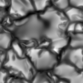
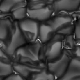
Figure 3: Upper panel : continuum emerging intensity of the last snapshot of the hydrodynamic simulation. The range is 0.65 to 1.4 the average emerging intensity. Lower panel : continuum emerging intensity of the last snapshot of the magnetohydrodynamic simulation. The range is 0.65 to 2.0 the average emerging intensity.

2.2 Solar secular evolution

We use a modified version ((2011)) of the hydrostatic one-dimensional CESAM code ((1997); Morel & Lebreton (2008)). CESAM’s calculations of the stellar interior rely on the usual ingredients of evolution codes:

The equation of state and opacities are the OPAL2005 ((1996); (2002)) ones for the (2009) (A09) metal repartition. Below $\rm logT=3.75$ we use the (2005) opacities for the same metal repartition.

The composition changes. The nuclear reaction rates are adapted from the NACRE compilation ((1999)). The nuclear network is restricted to the reactions relevant to the main sequence evolution : proton-proton chains and CNO cycles. In addition to the nuclear reactions the gravitational settling of elements is accounted for following the prescriptions of (1993). It results in the usual abundance decrease in the photosphere helium and metals mass fractions from the zero age main sequence (hereafter ZAMS) to the actual age.

The outer convection and atmosphere are handled in a less traditional manner, as we introduce prescriptions coming from Stagger 3-D calculations. However for the purpose of comparison, models relying on the usual 1-D convection prescriptions and atmospheres are also computed.

Surface and 1-D convection phenomenologies

The mixing length theory (hereafter MLT) and the phenomenology of (1996) (hereafter CGM) have been used for surface convection energy transfer and atmosphere calculation. As stressed by (2004) it is necessary to use the same phenomenology in the atmosphere and the interior. Therefore we consider different atmosphere grids depending on the underlying convection prescription. The approach is the same as in (2011) where the reader can find all the details of the implementation.

Both MLT and CGM atmosphere grid models were computed with the 1-D Atlas12 code atmosphere structure code ((2005)). Atlas12 calculates the non-grey atmosphere stratification. In both sets of atmosphere models, the current solar surface composition of A09 is considered and the convection characteristic length scale is $\rm 0.5H_{p}$ ((2006)). The atmosphere thermal gradient $\rm\nabla_{a}={dlnT}/{dlnP}$ is computed following the usual equation $\rm\nabla_{a}=\nabla_{rad}*\frac{df}{d\tau_{Ross}}$, $\rm\nabla_{rad}$ being the radiative diffusive gradient, and $\rm f(\tau_{Ross})$ the function relating effective temperature, optical depth and temperature: $\rm T^{4}=\frac{3}{4}T_{eff}^{4}f(\tau_{Ross})$. The outer boundary conditions to the internal structure in temperature and pressure are taken at the Rosseland optical depth 20. In order to obtain a smooth thermal gradient transition between the atmosphere and the interior the thermal gradient is linearly interpolated with respect to $\rm\tau_{Ross}$ between its atmosphere value $\rm\nabla_{a}$ and its interior value $\rm\nabla_{i}$: so that for $\rm 20<\tau_{Ross}<1$ we consider $\rm\nabla=x\nabla_{i}+(1-x)\nabla_{a}$ with $\rm x=\frac{\tau_{Ross}-1}{20-1}$.

Surface and 3-D convection simulations

Owing to their calculations, we dub the thermal gradients coming from the 3-D simulations the hydrodynamic and magnetohydrodynamic gradients, $\rm\nabla_{HYD}$ and $\rm\nabla_{MHD}$ respectively. These gradients are computed from the temperature and gas pressure of the 3-D simulations. In 1-D calculations, the turbulent pressure gradient is only accounted for in the equation of hydrostatic equilibrium. $\rm\nabla_{HYD}$ is obtained by horizontal and time averages of 3-D surface simulations including no magnetic field. Once we have ensured that this gradient is an average quantity relevant for solar evolution from ZAMS to the actual Sun (see §2.1) we introduce it in the stellar structure equations. We do not expect that accounting for the changes of surface conditions throughout solar history would greatly improve the results of this work. First these changes are moderate: the radius and the effective temperature increase by $\rm\approx 10\%$ and $\rm\approx 140K$ respectively from the solar ZAMS until today. More importantly the effects we investigate concern only the surface layers, they are not related to details of the inner structure resulting from the evolution of the Sun. Our results in §3.1 confirm that this is indeed the case. The average 3-D thermal gradient is introduced straightforwardly by considering that the temperature optical depth relation is $\rm\frac{dT}{dr}=\nabla_{HYD}\frac{T}{P}\frac{dP}{dr}$ (with T the temperature, r the radius and, P the gas pressure) between the Rosseland optical depths $10^{-4}$ and $10^{3}$. For $\rm\tau_{Ross}$ between $10^{3}$ and $10^{4}$ we base the thermal gradient on a linear interpolation with optical depth between $\rm\nabla_{HYD}$ and $\rm\nabla_{CGM}$: $\rm\nabla=x\nabla_{HYD}+(1-x)\nabla_{CGM}$ with $\rm x=\frac{10^{4}-\tau_{Ross}}{10^{4}-10^{3}}$ and $\rm\nabla_{CGM}$ the gradient computed in the phenomenology of (1996). We compute that at $\rm\tau_{Ross}=10^{3}$ ($\rm\approx 330\,km$ below the surface) the relative difference between $\rm\nabla_{HYD}$ and the adiabatic gradient $\rm\nabla_{ad}$ is about 15 percent (but much larger above as can be seen from Figure 4). Thus most of the superadiabatic effects are expected above this depth. At the same time the transition between the dynamical description of the temperature gradient and the CGM description is shallow enough to enable us to adjust the solar radius at solar age which is essential for the purpose of our work (see §2.3). The model buildt that way is called Solhyd. To investigate the surface magnetic effects on evolution we also build a model called Solmhd similar to Solhyd but where $\rm\nabla_{MHD}$ is used instead of $\rm\nabla_{HYD}$. Solhyd is calibrated following the procedure described in the next section.

2.3 Calibration and models surface properties

We consider that for the current Sun $\rm R_{\odot}=6.9566\,10^{10}cm$, $\rm L_{\odot}=3.846\,10^{33}erg.s^{-1}$ and a metal to hydrogen mass fraction $\rm Z/X=1.81\,10^{-2}$. In order to obtain these quantities in the models after 4.6 Gyr of evolution, we adjust their initial $\rm Z/X$, helium fraction and convective characteristic length scale. The chosen current radius obviously is a crucial parameter as of the calculation of eigenfrequencies. There are different definitions possible of it. What we consider here as the solar radius is the radius of the layer at effective temperature. Then $\rm R_{\odot}=6.9566\,10^{10}cm$ is the value recommended by (2008). It lies $\rm 330km$ below the commonly used value $\rm R_{\odot}=6.9599\,10^{10}cm$ ((1976)) and nearly corresponds to the seismic solar radius computed from f-modes whereas the (1976) radius agrees with the position of the inflexion point to the intensity profile at solar limb. The calibration is achieved to better than $10^{-6}$ in radius, luminosity and $\rm Z/X$. It is important to achieve such a high accuracy for the radius. The observed relative shifts of an eigenfrequency $\rm\nu$ between the solar maximum and minimum activity are the order of $\rm\Delta\nu/\nu=10^{-4}$. The eigenfrequency of a mode of radial order n depends on the stellar radius following $\rm\nu_{n}\approx n(2\int_{0}^{R_{\odot}}\frac{dr}{c_{s}})^{-1}$, with $\rm c_{s}$ the sound speed. Thus radii calibrated to much better than $\rm 10^{-4}$ are necessary to make sure that the differences calculated are not related to differences in the calibration radii. The solar model named Solmlt is based on the MLT. We obtain $\rm\alpha_{MLT}=2.45$ for it. This rather large value is required to achieve the actual solar radius because of the low $\rm\alpha_{MLT}=0.5$ in the atmosphere. Also considering $\rm\alpha_{MLT}=0.5$ in the atmosphere (2006) found $\rm\alpha_{MLT}=2.51$. For the model Solcgm, based on the CGM phenomenology, we have $\rm\alpha_{CGM}=0.785$.

For a model relying on the 3-D surface simulations, it is also possible to adjust the final radius, luminosity and composition at the same time provided the transition between the hydrodynamic thermal profile and the phenomenological one is not performed at too large an optical (or equivalently geometrical) depth. As mentioned at the end of the preceding section, the average 3-D temperature gradient is used down to $\rm\tau_{Ross}=10^{3}$. Below $\rm\tau_{Ross}=10^{4}$ we rely on the CGM phenomenology. A linear interpolation is performed between the two descriptions at intermediate optical depths (cf. §2.2). Doing so, almost all of the superadiabatic convection region is treated according to our 3-D prescriptions (see Figure 4). A smaller part of the superadiabatic region is still handled with the CGM. It is significant enough so that we keep a sufficient leverage on the deep convection zone specific entropy thanks to $\rm\alpha_{CGM}$ and therefore on the solar model radius. This is how Solhyd is buildt.

Figure 4: Thermal and adiabatic gradients in the superadiabatic layers of solar models as a function of the Rosseland optical depth. Solid line: average thermal gradient from 3-D simulations, dotted line: thermal gradient from the MLT phenomenology, dot-dashed line: thermal gradient from the CGM phenomenology, dashed line: adiabatic gradient.

Figure 5: Solid line : relative variation between averaged Rosseland opacity and Rosseland opacity of averaged density and temperature as a function of depth. Dashed line : relative variation between averaged $\rm\Gamma_{1}$ adiabatic index and $\rm\Gamma_{1}$ adiabatic index of averaged density and temperature as a function of depth. Note the different scales for the Rosseland opacity and the adiabatic exponent.

It is worth spending a few words on a model where the superadiabatic convection completely relies on 3-D simulations. If we perform the transition between the 3-D thermal gradient and the phenomenological CGM one between $\rm\tau_{Ross}=10^{6}$ and $\rm\tau_{Ross}=4\,10^{6}$ (near the lower boundary of the 3-D simulation box) the final radius becomes nearly insensitive to $\rm\alpha_{CGM}$. In such a full 3-D convection model changing $\rm\alpha_{CGM}$ from its solar calibration value 0.785 to 7.85 decreases the radius by $\rm 0.3\%$ only. As a comparison, in the models exclusively based on phenomenologies, the dependency on $\alpha$s is much larger : an increase of $\rm\alpha$ by 1 from the calibrated values reduces the radius by 6.3 and 8.5 percent in MLT and CGM models respectively. Unsurprisingly the radius of the full 3-D convection model departs from the solar radius at solar age. It is $\rm\approx 1.3\%$ above the actual solar radius. Considering that $\rm\alpha_{CGM}$ has no calibration effect on the model such a final radius is fairly close to the solar radius. Yet the difference is enough to shift the eigenfrequencies by more than 100 $\rm\mu Hz$ for modes of low-$\ell$ and radial order 15 to 30 thus masking the possible improvements brought by the implementation of 3-D effects.

Even though the thermal gradient and turbulent pressure accounted for in 1-D are estimated from 3-D simulations there are dimensional effects the 1-D cannot reproduce. As illustrated on Figure 5 the average subphotospheric opacity is significantly above the opacity corresponding to the average temperature and density (see R99; (2009)). This stems from the opacity’s strong dependence on temperature when $\rm H^{-}$ ions are its main contributor : namely $\rm\kappa\propto T^{10}$. The horizontally averaged opacity being larger in 3-D than in 1-D the subphotospheric temperature will be larger for the same total flux. The dimensional effects are to a lesser extent seen on EoS quantities such as the first adiabatic index $\rm\Gamma_{1}$ also shown on Figure 5. To take into account such 3-D effects directly we patched to 1-D solar structures the pressure, density, $\Gamma_{1}$ and Brunt-Väissälä frequency average vertical profiles from 3-D simulations. The procedure is similar to that adopted by R99 and is repeated for purely hydrodynamic and magnetohydrodynamic simulations in the models we called Solpatchs.

Table 1: Main properties of the models.

$$\begin{array}[]{lccccccccc}\hline\cr\vskip 3.0pt plus 1.0pt minus 1.0pt\cr\rm Name&\rm\nabla-type\,along\,evolution&\rm Temperature&\rm Turbulent&\rm Magnetic&\rm R_{T=5777}-R_{\odot}(km)&\rm R_{\tau=1}-R_{\odot}(km)\\ &&\rm and\,density&\rm pressure&\rm field&\\ \vskip 3.0pt plus 1.0pt minus 1.0pt\cr\hline\cr\vskip 3.0pt plus 1.0pt minus 1.0pt\cr\rm Solmlt&\rm\nabla_{MLT}&\rm No\,3-D\,effects&\rm No&\rm No&-5.85\,10^{-1}&-3.31\,10^{1}\\ \rm Solcgm&\rm\nabla_{CGM}&\rm No\,3-D\,effects&\rm No&\rm No&2.65\,10^{-1}&-3.31\,10^{1}\\ \rm Solhyd&\rm\nabla_{HYD}&\rm No\,3-D\,effects&\rm Yes&\rm No&6.50\,10^{-1}&-2.64\,10^{1}\\ \rm Solmhd&\rm\nabla_{MHD}&\rm No\,3-D\,effects&\rm Yes&\rm Yes&7.21\,10^{3}&7.18\,10^{3}\\ \rm Solpatch1&\rm\nabla_{HYD}&\rm 3-D\,effects&\rm Yes&\rm No&-3.91\,10^{-1}&-2.07\,10^{1}\\ \rm Solpatch2&\rm\nabla_{HYD}&\rm 3-D\,effects&\rm Yes&\rm Yes&-6.07\,10^{0}&-3.01\,10^{1}\\ \rm Solpatch3&\rm\nabla_{MLT}&\rm 3-D\,effects&\rm Yes&\rm No&-1.87\,10^{1}&-3.8910^{1}\\ \rm Solpatch4&\rm\nabla_{MHD}&\rm 3-D\,effects&\rm Yes&\rm Yes&-3.49\,10^{1}&-5.77\,10^{1}\\ \vskip 3.0pt plus 1.0pt minus 1.0pt\cr\hline\cr\end{array}$$

Table1 sums up the properties of the models we address in the remainder of this work. Col. 1 gives the model name, Col. 2 gives the convective thermal gradient used along solar evolution, Col. 3 indicates if the 3-D effects are accounted for directly (in the way mentioned just above), Col. 4 and 5 indicate respectively if turbulent pressure and magnetic fields are taken into account. Col. 6 gives the differences between the radius of the model at $\rm T=5777K$ and $\rm R_{\odot}$ (our reference solar radius assumed to be here $\rm R_{\odot}=6.9566\,10^{10}cm$). Col. 7 gives the differences between the radius of the model at $\rm\tau_{Ross}=1$ and $\rm R_{\odot}$. The models are calibrated in luminosity, radius, and $\rm Z/X$ to better than $\rm 10^{-6}$. However as Solmhd, Solpatch2, Solpatch3 and Solpatch4 have been buildt to explore the impact of the surface activity on the eigenfrequencies and the radius their radii are not calibrated with a similar accuracy. All the models have almost identical helium surface mass fractions ranging from Y=0.2349 to 0.2352, and also almost identical extent of the convection zone with radii of the base of the convection zone ranging from 0.7248 to 0.7249 $\rm R_{\odot}$. Let us finish this section with some important remarks on the models :

i) The near surface stratifications computed in 3-D are more extended than those in 1-D with the MLT or the CGM phenomenology. This is due to the larger subphotosperic temperatures required in 3-D than in 1-D atmosphere models to produce the same effective temperature (See R99 for a discussion of this effect) and to an additional lift provided by the turbulent pressure support. Thus the Solpatch1 model is not buildt from Solhyd directly but from a solar model evolved with the same outer convection prescription as Solhyd and whose photospheric radius is 115 km smaller than our calibration value. This procedure allowed us to adjust very accurately the Solpatch1 radius model to the solar radius. In Solpatch1 the outer pressure, density, $\Gamma_{1}$ and Brunt-Väissälä frequency vertical profiles are horizontal and time average of the purely hydrodynamic simulations down to our deepest layer of the 3-D hydrodynamic simulation at $\rm T=2.225\,10^{4}$K, $\rm\rho=2.657\,10^{-5}g.cm^{-3}$ and $\rm\tau_{Ross}=1.88\,10^{7}$. Therefore the 3-D effects are directly accounted for instead of being introduced indirectly through $\rm\nabla_{HYD}$ as in Solhyd. We stress that this patch procedure only concerns the solar age model, and not the solar evolution from ZAMS. The Solpatch3 model is buildt exactly as Solpatch1 but from a structure evolved with the MLT to a final radius 115 km smaller than Solmlt.

ii) The procedure to build Solpatch2 and Solpatch4 is similar to that for Solpatch1 except that the averaged surface vertical profiles from the magnetohydrodynamic simulations were used instead of the purely hydrodynamic profiles. These averages are considered down to our deepest layer of 3-D magnetohydrodynamic simulation at $\rm T=2.225\,10^{4}$K, $\rm\rho=2.647\,10^{-5}g.cm^{-3}$ and $\rm\tau_{Ross}=1.87\,10^{7}$. Both Solpatch1 and Solpatch2 result from the same evolutionary sequence based on $\rm\nabla_{HYD}$. However for Solpatch1 the patch at solar age is buildt from the hydrodynamic simulation whereas for Solpatch2 it is buildt from the magnetohydrodynamic one. Solpatch2 accounts for the magnetic effects around the actual solar surface but not for their feedback on the deeper structure during the solar evolution. On the contrary for Solpatch4, the structure is taken from a solar evolution model evolved with $\rm\nabla_{MHD}$ and the patch at solar age is made from the magnetohydrodynamic simulation. Therefore Solpatch4 accounts for both the magnetic effects on the current solar structure and during the solar evolution.

iii) The only difference between Solmhd and Solhyd are the thermal gradient and turbulent pressure. The purpose of Solmhd is to show the secular impact of magnetism on radius in the context of this work. Therefore Solmhd is not forced to solar radius at solar age by performing a calibration.

iv) Regarding the (purely) hydrodynamic modelling our approach resembles the approach of R99 and it is interesting to compare them. For instance both studies investigate how the change from MLT models to patched models affects the differences between the predicted and the observed eigenfrequencies. These differences stem from the incorrect modelling of the outer average structure of the Sun, what is referred to as the model effects. They also stem from the complex coupling of the modes with the radiative and convective fields, what is referred to as the modal effects. Contrary to R99 we don’t investigate both model and modal effects but only the model effects. Moreover our study is extended to models R99 did not address: the CGM model of convection (Solcgm) and the models based on realistic thermal gradients (Solhyd, Solmhd). Finally, R99 based most of their work on envelope models whereas we calculate the oscillations from models of the whole solar structure. For this series of reasons, the present study is complementary to the study of R99.

3 Results

We compute the eigenfrequencies of the previous models using the adipls package (made publicly available by J. Christensen-Dalsgaard from http://users-phys.au.dk/jcd/adipack.n/). Wave propagation is assumed adiabatic. We compare our theoretical frequencies to the Michelson Doppler Imager (MDI) observations described by (1998). The data have been retrieved from http://quake.stanford.edu/~schou/anavw72z/. We consider two sets of data: Smax, the first set, starts on August 27th 2001 and Smin, the second set, starts on December 12th 2008. Each set lasts 72 days. Smax is representative of solar maximum activity and Smin of solar minimum activity. For every model there are $\approx$ 150 modes for which we also have observational data. The orders go from 7 to 27, the angular degrees from 0 to 10 and the frequencies from from $\approx$1500 to $\approx$4300 $\mu$Hz.

3.1 Dynamical and phenomenological models

Figures 6 and 7 show the differences between model and observed frequencies. As is customary the differences have been scaled by $\rm Q_{nl}$ the ratio of the mode mass by the mode mass of the radial mode of same order. As the models we compare mainly differ in their surface layers, and we only compare lower degree modes, the scaled frequency differences are expected to be predominantly functions of frequency.

Figure 6: Differences between models and observed eigenfrequencies as a function of the observed eigenfrequencies. + : model Solmlt. $\rm\diamond$ : model Solcgm. $\rm\triangle$ : model Solhyd. The average errobar on observed frequencies is $\rm\approx 0.06\,\mu Hz$ which is smaller than the symbol sizes.

Figure 7: Differences between models and observed eigenfrequencies as a function of the observed eigenfrequencies. $\rm\square$ : model Solpatch1. $\rm\times$ : model Solpatch2. The Solpatch1 model is compared to the Smin eigenfrequencies set representing the solar minimum whereas the Solpatch2 model is compared to the Smax eigenfrequencies set representing the solar maximum.

Figure 6 shows the effects of changes in the treatment of thermal gradient and the turbulent pressure in the superadabatic region. The modelled eigenfrequencies agree with the observations up to $\rm\sim 3000\,\mu$Hz. Then they become larger than the observed ones with discrepancies increasing towards higher frequencies. At $\rm\sim 4000\,\mu$Hz the MLT convection model and the CGM model exhibit frequencies about 5 $\mu$Hz larger than the observed ones and the frequencies of the model based on $\rm\nabla_{HYD}$ differ from the observed ones by about $\rm 8\,\mu$Hz. These results suggest that the differences between observed and theoretical frequencies are not due to an incorrect calculation of the average thermal gradient. Solmlt and Solcgm exhibit quite different gradients (see Figure 4) but have similar eigenfrequencies. In spite of a gradient probably closer to the real one than Solmlt or Solcgm, the Solhyd model has eigenfrequencies that are not in better agreement with the observations. This suggests that the ability of a model to predict the correct eigenfrequencies is not only related to its ability to reproduce the correct average thermal gradient and the turbulent pressure. Figure 6 and Figure 1 of R99 compare the differences between the eigenfrequencies of models based on the MLT and observed eigenfrequencies. Both plots show that the predictions agree with observations at low frequency and become increasingly too large above a certain threshold. The thresholds differ. When focusing on the low $\ell$ p-modes of Figure 1 of R99 (corresponding to the modes we compute) we note that our MLT model is in agreement with the observations over a larger frequency range. Namely, at $\rm 3000\,\mu\,Hz$ and $\rm 4000\,\mu\,Hz$ R99 report discrepancies of $\rm\sim 5\,\mu\,Hz$ and $\rm\sim 12\,\mu\,Hz$ respectively whereas we report discrepancies of $\rm\sim 1\,\mu\,Hz$ and $\rm\sim 5\,\mu\,Hz$ respectively. We do not know the origin of this improvement.

Figure 7 compares models Solpatch1 and Solpatch2 showing the improvement brought by direct patchs of the 3-D simulations average structure. Solpatch1 and Solpatch2 are compared to the Smin and Smax set of data respectively. These models frequencies predictions are less than $\rm 3\,\mu$Hz below the observations at $\rm\sim 3000\,\mu$Hz. This is their largest departure from the observed frequencies. At higher frequency the difference decreases below $\rm 1\,\mu$Hz. This results stresses the importance of accounting for the 3-D nature of surface convection and not only for the correct thermal gradients and turbulent pressure when it comes to estimating the solar/stellar absolute oscillation frequencies. If here again we want to compare our results with R99, Figure 7 will obviously correspond to Figure 6 of these authors. The models that are addressed in both cases are made of patchs of 3-D simulations averages. Interestingly, the differences computed with the observed eigenfrequencies have similar shapes. For frequencies below $\rm\sim 4000\,\mu$Hz we compute eigenfrequencies smaller than the observed ones with a maximum difference of $\rm\sim 3\,\mu$Hz. Similarly, for frequencies below $\rm\sim 3500\,\mu$Hz, R99 compute eigenfrequencies smaller than the observed ones. The maximum difference they compute is larger than in our work: $\rm\sim 4\,\mu$Hz. Above $\rm\sim 3500\,\mu$Hz the eigenfrequencies of the R99 work become larger than the observed ones. Using our numerical tools we were unfortunately unable to determine oscillation frequencies towards the larger frequencies, but it is clear from Figure 7 that a similar trend as in R99 is expected.

Let us now review three possible causes of the remaining differences between the eigenfrequencies of the patched models Solpatch1 and Solpatch2 and the observations: the assumption made to buildt the solar evolution models, the solar radius that is considered and, the uncertainties on the physics of the modes.

First, how are our results sensitive to the hypotheses on the surface convection adopted in the solar evolution models? Figure 8 shows that the type of convection chosen to perform the past solar evolution has a small impact on the seismic surface term of the present day Sun. The models Solpatch1 and Solpatch3 correspond to patches of the same averaged atmosphere structure onto different solar interior structures. These structures correspond respectively to solar evolution models using $\rm\nabla_{HYD}$ and $\rm\nabla_{MLT}$. Yet Solpatch1 and Solpatch3 frequency differences are $\rm 1\,\mu$Hz at most. As mentioned in §2.2 this suggests that using a series of convection models to follow the varying surface conditions along the main sequence would probably make little difference for eigenfrequencies—at least in the solar case. Figure 8 also estimates how the eigenfrequencies change provided the surface magnetic activity is accounted for during the solar evolution. In the Solpatch4 case, the evolution uses $\rm\nabla_{MHD}$. The eigenfrequencies of this model are almost identical to those of Solpatch2 model whose evolution uses $\rm\nabla_{HYD}$.

The models eigenfrequencies depend on the current global parameters adopted and especially the radius. How would a change of the calibration radius affect the calculated eigenfrequencies? This is an interesting question firstly in the perspective of asteroseismic investigations in other solar-type stars for which the radius is known with much less precision. Secondly because the value of the solar radius is not completely settled. For the solar effective temperature layer, (1998) estimate $\rm R_{\odot}=6.9551\,10^{10}cm$ but it could be up to $\sim 300$ km larger with $\rm R_{\odot}=6.9578\,10^{10}cm$ ((1998)). Our calibration value stands inbetween at $\rm R_{\odot}=6.9566\,10^{10}cm$ but we also computed the eigenfrequencies of a model calibrated on a radius that is 300 km larger (and is therefore almost calibrated on the (1976) radius). This model was buildt in the same manner as Solpatch1 with the only difference of its radius. We found that its eigenfrequencies are changed by $\rm 2\,\mu$Hz at most with respect to Solpatch1. Above $\rm 2500\,\mu$Hz the frequency shift induced by photospheric radius change is almost constant while it is negligible below $\rm 2000\,\mu$Hz.

Last but not least, the physics of the modes in the outer layers is an obvious possible culprit of the observations/predictions differences remaining in Figure 7. Our work however suggests that this contribution is not the major one. Indeed R99 tried to approximate the modal effects whereas we completely ignore them and nevertheless our calculations show a better agreement to the observations. Thus we tend to think that a large part of the lingering difference between models and observations does not originate from the modal effects but from other physical processes to be included in the model effects: the rotation, the large scale convective and meridional flows, the role of the magnetic field that is present even in the quiet Sun.

Figure 8: Differences between models eigenfrequencies as a function of their eigenfrequencies. $\rm\square$: model Solpatch1 minus model Solpatch3 frequencies. $\rm\times$ : model Solpatch2 minus model Solpatch4 frequencies.

3.2 Activity impact

In our magnetohydrodynamic run the induction equation is solved throughout all the domain and simulation duration. The plasma entering the simulation box from below carries a 1.2 kG horizontal magnetic field. This configuration is inspired from (2009) as their helioseismic analysis suggests that the toroidal magnetic field at $\rm 0.996\,R_{\odot}$ (i.e. 3000 km below the surface) is about 1.2 kG at maximum solar activity. The simulated magnetic field has an impact on both the absolute radius of the Sun and its seismic properties.

Let us first examine the activity impact on the radius. In the following the relative MHD/HYD variation considered is $\rm\delta x/x=(x_{MHD}-x_{HYD})/x_{HYD}$ for any quantity x. Figure 9 illustrates the Lagrangian relative radius variation $\rm\delta_{m}r/r$ (i.e. the relative radius variation throughout layers corresponding to the same mass coordinate) between the purely hydrodynamic 3-D (Solpatch1) and the magnetohydrodynamic 3-D simulations (Solpatch2). The radius variation is most significant in the $\rm\sim 900km$ region extending above the solar photosphere. Here we are, however, only concerned in the solar interior. For the solar interior the contraction is most significant with $\rm\delta_{m}r/r\sim-2\,10^{-5}$ at the surface and within the first 200 km below it. The shrinking clearly corresponds to a sharp drop in the turbulent pressure support. The turbulent pressure gradient also changes deeper than 200 km, yet in those underlying regions the ratio of turbulent pressure gradient to gas pressure gradient becomes negligible and so are the effects of its change (see also Eqs. 12 and 15 of (2006)). For this reason we have drawn in Figure 9 the relative variation of the vertical turbulent pressure gradient when the magnetic field is accounted for ($\rm(\nabla P_{turb}^{MHD}-\nabla P_{turb}^{HYD})/\nabla P_{turb}^{HYD}$) multiplied by the ratio of turbulent pressure gradient to gas pressure gradient ($\rm\nabla P_{turb}^{HYD}/\nabla P_{gas}^{HYD}$). The Figure also shows the impact of magnetism on sound speed. Right beneath the surface the sound speed $\rm c_{s}$ increases the order of $\rm 1\%$. In order to keep the same ordinate axis scale for all the quantities shown on Figure 9, the turbulent pressure gradient and the sound speed variations have been scaled by $\rm 5\,10^{-4}$ and $\rm-2\,10^{-3}$ respectively. The correlation between the variation of turbulent pressure support and radius and the anti-correlation between the variation of turbulent pressure support and sound speed are striking. Figure 10 shows the relative variations of pressure, density, sound speed $\rm c_{s}$, and $\rm\upsilon=\frac{\Gamma_{1}}{c_{s}}$, $\rm\Gamma_{1}$ being the first adiabatic index. Deeper than 1000 km below $\rm R_{\odot}$ the changes in any of these quantities become rapidly negligible. Between 1000 and 200 km below $\rm R_{\odot}$ pressure and density increase altogether which results in a nearly constant sound speed and $\rm\upsilon$. Finally from 200 km below $\rm R_{\odot}$ up to the surface $\rm c_{s}$ increases because of pressure increase and constant density and in spite of a decreased first adiabatic index $\rm\Gamma_{1}$. $\rm\upsilon$ exhibits a sharp drop.

Before moving to the seismic effects let us comment on the impact of activity on the observed radius. A stellar radius may be defined in many ways. We have considered the solar calibration radius to be the radius of the effective temperature layer but we report on the changes in both this radius and the radius of the $\rm\tau_{Ross}=1$ layer in Table 1. From the model Solpatch1 to Solpatch2 we compute that the shells at effective temperature and $\rm\tau_{Ross}=1$ go down by respectively 5.7 km and 9.4 km. As Solpatch1 and Solpatch2 are obtained from the same evolutionary sequence, we therefore estimate that the immediate effect of the magnetic activity on the structure is to decrease the radius by 8 milliarcseconds (hereafter mas) at the effective temperature layer and 14 mas at $\rm\tau_{Ross}=1$. Note that the effective temperature layer lies at $\rm\tau_{Ross}\approx 0.55$ in the photosphere and that consequently we predict that the radius variation increases with depth in the visible part of the atmosphere. The predicted radius changes will be difficult to detect because they remain smaller than the constant fluctuations of depth induced by convective overshooting or p-modes oscillations: the order of 30 km for the effective temperature layer. If the immediate effect of surface magnetism is to decrease the radius we compute that its secular effect is on the contrary to increase it in agreement with other works ((1995); (2010)). There is no contradiction in this. Solmhd has a much larger radius than Solhyd because of a slightly larger specific entropy of its deep convection zone. The difference stems from $\rm\nabla_{HYD}$ and $\rm\nabla_{MHD}$: when we perform the downward integration of these thermal gradients starting from the same surface conditions ($\rm T=5777$ K and $\rm\rho=2.5\,g.cm^{-3}$) we end up on an adiabat that is $\rm\approx 1.96\,10^{7}erg.K^{-1}.g^{-1}$ higher in specific entropy in the magnetohydrodynamic case than in the purely hydrodynamic case. Magnetic fields impede convective motions (see §2.1) and eventually convection becomes less efficient. Actually Solhyd and Solmhd deep convection zone specific entropies differ only by $\rm\Delta s=7.90\,10^{6}erg.K^{-1}.g^{-1}$ because as mentioned in §2.2 their thermal gradients exclusively rely on $\rm\nabla_{HYD}$ and $\rm\nabla_{MHD}$ only down $\rm\tau_{Ross}=10^{3}$. The time required for the solar luminosity to change the specific entropy from the Solhyd value to the Solmhd value is $\rm\Delta s\int_{CZ}Tdm/L_{\odot}\approx 3500$ yr where the integration is made over the convection zone with T the temperature, and dm the mass increment. Therefore the duration of a cycle is much too short for the change in the outer gradient to affect the thermal structure deeper down and eventually increase the radius.

Figure 9: Relative Lagrangian variations $\rm\delta_{m}x/x=(x_{MHD}-x_{HYD})/x_{HYD}$ as a function of radius between models Solpatch1 and Solpatch2. Solid line: radius variation, dashed line: sound speed variation times $\rm-2\,10^{-3}$, dotted line: turbulent pressure variation times $\rm 5\,10^{-4}\nabla P_{turb}^{HYD}/\nabla P_{gas}^{HYD}$.

Figure 10: Relative Lagrangian variation $\rm\delta_{m}x/x=(x_{MHD}-x_{HYD})/x_{HYD}$ as a function of radius between models Solpatch1 and Solpatch2. Solid line: $\rm\upsilon$, dotted line: density, dashed line: pressure, dot-dashed line: sound speed.

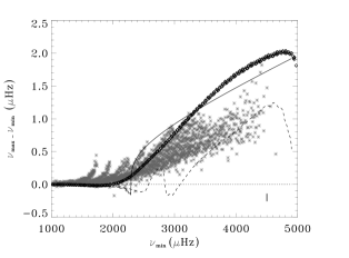
Figure 11: $\rm\diamond$: frequency shift between models Solpatch1 and Solpatch2 as a function of frequency. Solid line: frequency shift computed from Equation 1 and cut-off frequency from Equation 3, Dashed line: frequency shift computed from Equation 1 and cut-off frequency from Equation 2. Dotted line: frequency shift computed from the Equation 1 $\rm\frac{\delta_{m}r}{r}$ term. Grey crosses: observed frequency shifts for p-modes. The average errorbar on frequency shifts $\rm 0.06\,\mu Hz$ is shown at the lower right part of the plot.

Figure 12: Left hand ordinate axis: cut-off frequency from equation 1 vs radius (solid line). cut-off frequency estimate from equation 2 vs radius (dashed line). Right hand ordinate axis: turbulent pressure gradient to gas pressure gradient ratio vs radius (dotted line). All the physical quantities of this Figure are related to the Solpatch1 model.

The frequencies of solar p-modes are observed to change with phase of the solar activity cycle. From minimum to maximum solar activity (2007) and (2008) report frequency increases of 0.3 to 0.4 $\mu$ Hz around 3000 $\mu$Hz. Figure 11 shows the differences between 1928 modes of the Smin and Smax datasets. The observed frequencies ranges from $\rm 1025\,\mu Hz$ to $\rm 4644\,\mu Hz$, the radial order from 0 to 27, and the degree from 0 to 298. In this data sample the activity related shifts increase with frequency to reach $\rm 1\mu$Hz at 4000 $\mu$Hz. We drawn in overplot the eigenfrequency differences between models Solpatch1 ($\rm\nu_{min}$) and Solpatch2 ($\rm\nu_{max}$). Note that the modal magnetic effects are not included in our theoretical p-modes calculation, the changes in eigenfrequencies only results from the changes in the near surface structure. The models predict no frequency variations below $\rm\sim 2200\,\mu Hz$ and actually they can predict no variation below $\rm\sim 1800\,\mu Hz$ as this is the cut-off frequency at the base of our hydrodynamic/magnetohydrodynamic simulations. Small eigenfrequency changes the order of $\rm 0.3\mu$Hz are seen in the data at low frequency. Magnetic activity effects extending deep in the convection zone could explain them ((2008)). Above $\rm\sim 2200\,\mu Hz$, the activity related frequency shift increases nearly linearly up to $\rm\sim 4000\,\mu Hz$ : the slope is $\rm 10^{-3}\,\mu Hz/\mu Hz$. The amplitude of the observed frequency shift is about two thirds of our predictions. At $\rm 3000\,\mu Hz$ the average shift from the data we use is $\rm 0.51\,\mu Hz$ in the $\rm 3000\pm 50\,\mu Hz$ bin while our calculation gives $\rm 0.75\,\mu Hz$. Given the spread in the observed frequency shifts the models predictions are actually compatible with the upper envelope of them. At frequencies higher than $\rm\sim 4000\,\mu Hz$ the difference reaches a maximum of $\rm 2\,\mu Hz$ at $\rm\sim 4800\,\mu Hz$ and then shows a slight decline.

(1997) have related the changes in their surface models properties to the variations of their eigenfrequencies through

$$\begin{multlined}\frac{\delta\nu}{\nu}\approx\Big{(}\int_{0}^{R_{c}}(1-\frac{\nu_{c}^{2}}{\nu^{2}})^{1/2}[\frac{\delta_{m}r^{2}P}{r^{2}P}-2\frac{\nu_{c}^{2}}{\nu^{2}}(1-\frac{\nu_{c}^{2}}{\nu^{2}})^{-1}\frac{\delta_{m}r}{r}]\frac{dr}{c_{s}}\\ {+\int_{0}^{R_{c}}(1-\frac{\nu_{c}^{2}}{\nu^{2}})^{-1/2}\frac{\delta_{m}\upsilon}{\upsilon}\frac{dr}{c_{s}}\Big{)}/\int_{0}^{R_{c}}(1-\frac{\nu_{c}^{2}}{\nu^{2}})^{-1/2}\frac{dr}{c_{s}}}\end{multlined}\frac{\delta\nu}{\nu}\approx\Big{(}\int_{0}^{R_{c}}(1-\frac{\nu_{c}^{2}}{\nu^{2}})^{1/2}[\frac{\delta_{m}r^{2}P}{r^{2}P}-2\frac{\nu_{c}^{2}}{\nu^{2}}(1-\frac{\nu_{c}^{2}}{\nu^{2}})^{-1}\frac{\delta_{m}r}{r}]\frac{dr}{c_{s}}\\ {+\int_{0}^{R_{c}}(1-\frac{\nu_{c}^{2}}{\nu^{2}})^{-1/2}\frac{\delta_{m}\upsilon}{\upsilon}\frac{dr}{c_{s}}\Big{)}/\int_{0}^{R_{c}}(1-\frac{\nu_{c}^{2}}{\nu^{2}})^{-1/2}\frac{dr}{c_{s}}}$$ (1)

with $\rm\delta\nu/\nu$ the relative frequency variation, $\nu_{c}$ the cut-off frequency, P the pressure, r the radius, $\rm c_{s}$ the sound speed, and $\rm\upsilon=\Gamma_{1}/c_{s}$. $\rm\delta_{m}$ stands for the Lagrangian variations of the physical quantities and $\rm R_{c}$ for the cut-off radius. Using this equation we will now outline some interesting features in our models. The dotted line in Figure 11 shows that we expect no visible eigenfrequency changes if the only term taken into account in Equation 1 is $\rm\frac{\delta_{m}r}{r}$. This could be anticipated as with $\rm\frac{\delta_{m}r}{r}=1.7\,10^{-5}$ at most in the interior (Figure 9), the radius variations are tiny. We find that the largest variation of the cut-off radius occurs for $\rm\nu_{c}=5000\,\mu Hz$ and is $\rm\frac{\delta R_{c}}{R_{c}}=5\,10^{-6}$. These results suggests that the frequency variations are not related to variations of the radius of the acoustic cavity but are related to changes inside the acoustic cavity: changes in pressure and $\rm\upsilon$.

The dashed line in Figure 11 shows the eigenfrequencies variations calculated from Equation 1 provided the cut-off frequency $\nu_{c}$ is computed using the pressure scale height $\rm H_{p}$ as is frequently done:

$$\rm 2\pi\nu_{c}\approx\frac{c_{s}}{2H_{p}}$$ (2)

The shape of the line is directly related to the shapes of $\rm\frac{\delta_{m}\upsilon}{\upsilon}$ and $\rm\frac{\delta_{m}P}{P}$ seen on Figure 10. In particular the change of sign in the predicted eigenfrequency variation at about $\rm 2800\,\mu$Hz is related to the marked drop in $\rm\frac{\delta_{m}\upsilon}{\upsilon}$ that can be seen at $\rm 0.9998\,R_{\odot}$ in Figure 10. Figure 12 shows that the cut-off frequency computed from Equation 2 nearly is $\rm 2800\,\mu$Hz at $\rm 0.9998\,R_{\odot}$.

Using the pressure scale height in cut-off frequency calculation actually is an approximation. The correct formula for cut-off frequency is based on $\rm H_{\rho}$, the density scale height ((1984)):

$$\rm 4\pi^{2}\nu_{c}^{2}=\frac{c_{s}^{2}}{4H_{\rho}^{2}}(1-2\frac{dH_{\rho}}{dr})$$ (3)

The solid line in Figure 11 shows the eigenfrequencies variations calculated from Equation 1 using this cut-off frequency. In this case there is no sign change in the eigenfrequency variation as in the preceding case. There are two reasons for this. First, as shown in Figure 12 the cut-off frequency computed from Equation 3 becomes zero on the $\rm[0.9996,0.9998]\,R_{\odot}$ interval. Consequently, the eigenfrequency variations are less sensitive to the $\rm\frac{\delta_{m}\upsilon}{\upsilon}$ and more sensitive to $\rm\frac{\delta_{m}P}{P}$ changes than when the Equation 2 is used for the cut-off frequency. Second, the acoustic cavity is smaller than $\rm 0.9999\,R_{\odot}$ at any frequency whereas it clearly extends above $\rm 1.0005\,R_{\odot}$ when the Equation 2 is used for cut-off frequency. Figure 11 shows that the calculation based on the correct cut-off frequency is in better agreement with the observations (or the direct calculation of variations) than the calculation based on the approximated cut-off frequency. In the context of activity related shifts one should not use the pressure scale height to calculate an approximate cut-off frequency because it strongly differs from the exact cut-off frequency (Figure 12). There is an interesting consequence to this as, provided the Equation 3 is used for cut-off frequency calculation, the eigenfrequencies variations become mostly sensitive to pressure changes.

4 Conclusion

We have addressed the effects of surface convection and magnetism modelling on the solar models p-modes frequencies and radii. We used a 1-D code to follow the evolution of the whole Sun from ZAMS until now and a 3-D code to simulate its current magnetoconvection over 4 Mm around the surface. Different prescriptions for the surface convection were adapted to the stellar evolution code: the MLT, the CGM phenomenology, and averaged stratifications from our 3-D simulations. In our magnetic simulation runs a 1.2 kG horizontal field is carried by the incoming fluid at the lower boundary of the domain. This configuration mimics the 1.2 kG toroidal field suggested by the seismic analysis of (2009) at $\rm 0.996R_{\odot}$ and for maximum activity. We compared the eigenfrequencies of the models to recent observations for about 150 eigenfrequencies. We also discussed the changes in modelled radius with activity. Our results are as follows:

Convection hydrodynamics and seismology

For any of the adopted surface convection the models predict the solar p-modes eigenfrequencies within $\rm 2\,\mu$Hz up to $\rm\approx 3000\,\mu$Hz. The situation changes above that value: both the MLT and the CGM phenomenologies show comparable trends to overestimate the eigenfrequencies. The CGM phenomenology provides a slightly better agreement with the observations because its superadiabatic region is very narrow and the superadiabaticity very intense. Because of that, the turbulent pressure of the CGM model expands the acoustic cavity which leads to frequencies in slightly better agreement with the observations than in the MLT case. However the CGM phenomenology thermal gradient is much larger than what is suggested by the 3-D calculations while the MLT superadabatic gradient is comparable to them. When the subsurface thermal gradient is adapted from the averaged 3-D calculations and the turbulent pressure is accounted for, the predicted frequencies are higher than those of the models relying on the MLT or the CGM. The situation only improves if the surface layers pressure, density and first adiabatic index are directly taken from the averaged 3-D computations. This is in good agreement with the results of (1999) who performed similar patchs. But, in addition to this previous work, it also outlines that accounting for the correct outer structure in the context of 1-D solar evolution does not produce better results than the usual phenomenologies. In the so-called patched models the computed eigenfrequencies remain very close to and slightly below the observed ones in the frequency domain above 3000 $\rm\mu Hz$. The improvement brought by these patched models weakly depends on the outer convection model (phenomenological or based on simulations) used to perform the preceding solar evolution to obtain the deeper solar structure. The hydrodynamic models that are patched do not account for magnetic activity. Accounting for it even at the moderate level of solar minimum would increase the eigenfrequencies and improve further the agreement with observations. For the patched models, the mean pressure, mean first adiabatic index, mean density and, mean energy are not related by the equation of state. Because of their non-linear relationships the average of the local values is not equal to the equation of state values of the means. For the same reason, the average opacity is not the opacity computed from the average temperature and density.

Activity and radius

For a given solar interior structure, when the surface layers are patched from the magnetohydrodynamic simulation instead of the hydrodynamic one the effect is a $\rm 1.7\,10^{-5}$ Lagrangian radius relative decrease at the surface and directly below. This corresponds to a $\rm\approx 12$ km shrinking of the mass layers at surface but only translates into a $\rm\approx 6$ km shrinking of the effective temperature layer (or $\rm\approx 10$ km shrinking of the optical depth layer at $\rm\tau_{Ross}=1$). The difference stems from the Lagrangian relative variations of temperature and density near the surface (that are considerably larger than $\rm 1.7\,10^{-5}$, see (1997)). They induce an opacity increase at a given mass coordinate which attenuates the Lagrangian radius decrease. The radius of a layer at a given optical depth is related to both its geometrical depth and to the opacity variations of the overlying regions. One should keep in mind that these results only concern the effects of activity modelled in the $\rm 4\,10^{-3}R_{\odot}=3Mm$ region immediately below the surface. f-modes have indeed shown that radius variations occur in deeper regions and down to $\rm 0.97R_{\odot}$ ((2005)). Obviously these variations could also affect the visible radius. However the surface activity affects the atmosphere relative stratification and this is perhaps less sensitive to the physics of the deeper regions. From the optical depth point of view our simulations suggest that the radius contraction with activity should increase with depth on the $\rm 10^{-1}\leq\tau_{Ross}\leq 1$ range. For instance, we predict that the distance between the layer at $\rm\tau_{Ross}\approx 0.55$ (T=5777 K) and the one at $\rm\tau_{Ross}=1$ increases from 20 km with no activity to 24 km with activity: that is a 6 mas difference.

Activity and seismology

We computed the changes in eigenfrequencies when the magnetic activity is accounted for and compared them to the differences observed between activity maximum and minimum. Our calculations reproduce the order of magnitude and frequency dependence of frequency changes along the Hale activity cycle. No variation is predicted below $\rm 2200\,\mu Hz$. From this point on, the shift increases almost linearly to reach $\rm 1.7\,\mu Hz$ at 4000 $\rm\mu Hz$. The frequency increase is not related to a change in the size of the acoustic cavity but mostly to a thermal pressure increase in a $\rm 10^{-3}\,R_{\odot}$ layer starting right below the solar surface at $\rm R_{\odot}=6.5966\,10^{5}\,km$. The observed frequency shifts are spread and our calculations correspond nearly to the upper envelope of the observations. There might be several reasons to the slight overestimation of frequency shifts. The simulated incoming magnetic field may be too strong. Secondly, we did not explore the impact of the poloidal component of the magnetic field which would be introduced as a vertical component of the incoming field in our geometry. In other words our incoming field configuration is perhaps too simple. Thirdly, the models we use for frequency variations are 1-D, we do as if the toroidal field at $\rm 0.996R_{\odot}$ had the same intensity whatever the latitude. Fourthly, all the rotation effects such as the meridional flow are ignored and the simulation box is too small for the mesogranular or supergranular scales to be accounted for. Finally, by comparing the purely hydrodynamic model to the magnetohydrodynamic one we completely ignore the magnetic field effects at the cycle minimum which leads to an overestimated minimum to maximum contrast. It is clear that a lot more investigations need to be done.

3-D simulations of solar surface convection have been known for some time to diminish the seismic surface term. This work shows that above $\rm 2200\,\mu Hz$ the magnetic activity has a potential impact of the order of a $\rm 1\,\mu Hz$ on the eigenfrequencies. This is the order of the observed shifts along solar cycle. This is also the order of the differences between the observed frequencies and those computed from 3-D simulations without any magnetic field. Thus further efforts in explaining the solar surface term should now take into account the effects magnetic activity even in moderately active stars such as our Sun.

References

- (1) Allen, C. W., 1976, Astrophysical Quantities (3rd ed.; London: Athlone)
- (2) Angulo, C., et al., Nucl. Phys. A656 (1999)3-187
- (3) Antia, H.M., 1998, A&A 330, 336
- (4) Asplund, M., Grevesse, N., Sauval, J., 2005, ASP Conference Series, Vol XXX.
- (5) Asplund, M. Grevesse, N. Sauval, A. J, Scott, P., 2009, A&RAA, 47, 981
- (6) Baldner, Charles S., Antia, H. M., Basu, Sarbani, Larson, Timothy P., 2009, ApJ, 705, 1704
- (7) Basu, S., Antia, H. M., Tripathy, S. C., 1999, ApJ, 512, 458
- (8) Beeck, B., Collet, R., Steffen, M., Asplund, M., Cameron, R. H., Freytag, B., Hayek, W., Ludwig, H.-G., Schüssler, M., 2012, A&A, 539, 121
- (9) Böhm-Vitense, E., 1958, Zs. f. Ap., 46, 108
- (10) Brown, T. M., Christensen-Dalsgaard, J., 1998, ApJ, 500, 195
- (11) Canuto, V. M., Goldman, I., Mazzitelli, I., 1996, ApJ, 473, 550
- (12) Castelli, F., Mem. S.A.It. Suppl., 2005, 8, 25
- (13) Chaplin, W. J., Elsworth, Y., Miller, B. A., Verner, G. A., New, R., 2007, ApJ, 659, 1749
- (14) Christensen-Dalsgaard, J., Nuclear Physics B, 48, 325
- (15) Christensen-Dalsgaard, J., Thompson, M.J., 1997, MNRAS 284, 527
- (16) Collet, R., Hayek, W., Asplund, M., Nordlund, A., Trampedach, R., Gudiksen, B., 2011, A&A, 528, 32
- (17) Corbard, T., Thompson, M. J., 2002, Sol Phys 205, 211
- (18) Deubner, F.-L., Gough, D., 1984, ARA&A 22, 593
- (19) Feautrier, P., 1964, Comptes Rendus Acad. Sci. Paris, 258, 3189
- (20) Ferguson, J. W., Alexander, D. R., Allard, F., Barman, T., Bodnarik, J. G., Hauschildt, P. H., Heffner-Wong, A., Tamanai, A., 2005, ApJ, 623, 585
- (21) Gustafsson, B., Bell, R. A., Eriksson, K., Nordlund, A., 1975, A&A, 42, 407
- (22) Haberreiter, M., Schmutz, W., Kosovichev, A. G., 2008, ApJ, 675, 53
- (23) Lefebvre, S., Kosovichev, A., G., ApJ, 633, 149
- (24) Ludwig, H.G., Allard, F., Hauschildt, P. H., 2006, A&A, 459, 599
- (25) Ludwig, H.G., Allard, F., Hauschildt, P. H., 2002, A&A, 395, 99
- (26) Lydon, T., Sofia, S., 1995, ApJS, 101, 357
- (27) Macdonald, J., Mullan, D. J., 2010, ApJ, 723, 1599
- (28) Proffitt, C. R., Michaud, G., 1993, ASP Conference Series, Vol. 40, 246
- (29) Montalban, J., D’Antona, F., Kupka, F., Heiter, U., 2004, A&A, 416, 1081
- (30) Morel, P., 1997, A&AS, 124, 597
- Morel & Lebreton (2008) Morel, P., Lebreton, Y., 2008, Ap&SS, 316, 61
- (32) Mullan, D. J., MacDonald, J., Townsend, R. H. D., 2007, ApJ, 670, 1420
- (33) Nordlund, Ake, Stein, Robert F., Asplund, M., 2009, LRSP, 6, 2
- (34) Nordlund, A., 1982, A&A, 107, 1
- (35) Piau, L., Ballot, J., & , Turck-Chièze, S., 2005, A&A, 430, 571
- (36) Piau, L. Kervella, P., Dib, S., Hauschildt, P., 2011, A&A, 526, 100
- (37) Rabello-Soares, M. C., Korzennik, S. G., Schou, J., 2008, Sol. Phys., 251, 197
- (38) Robinson, F. J., Demarque, P., Li, L. H.,Sofia, S., Kim, Y.-C., Chan, K. L., Guenther, D. B., 2003, MNRAS, 340, 923
- (39) Rogers, F. J.,Swenson, Fritz J., Iglesias, Carlos A., 1996, ApJ 456, 902
- (40) Rogers, F. J., Nayfonov, A., ApJ 576, 1064
- (41) Rosenthal, C. S., Christensen-Dalsgaard, J., Nordlund, A., Stein, R. F., Trampedach, R., 1999, A&A, 351, 689
- (42) Samadi, R., Kupka, F., Goupil, M. J., Lebreton, Y., van’t Veer-Menneret, C., 2006, A&A, 445, 233
- (43) Schou, J., 1999, ApJ, 523, 181
- (44) Skartlien, R., ApJ 536, 465
- (45) Stein, R.F., Nordlund, A., 1998, ApJ, 499, 914
- (46) Stein, R.F., Nordlund, A., 2006, ApJ, 642, 1246
- (47) Stein, R.F., Lagerfjard, A., Nordlund, A., Georgobiani, D., 2011, Sol. Phys., 268, 271
- (48) Stein, R.F., Nordlund, A., 2012, ApJ, 753, 13
- (49) Trampedach, R., Däppen, W., Baturin, V. A., 2006, ApJ 646, 560.
- (50) Trampedach, R., Asplund, M., Collet, R., Nordlund, A., Stein, R. F., 2013, ApJ 769, 18
- (51) Turck-Chièze, S., Basu, S., Brun, A. S., Christensen-Dalsgaard, J., Eff-Darwich, A., Lopes, I., Pérez Hernández, F., Berthomieu, G., Provost, J., Ulrich, R. K., and 9 coauthors, 1997, Sol. Phys. 175, 247