Geometric Results for Compressible Magnetohydrodynamics

Abstract

Recently, compressible magnetohydrodynamics (MHD) has been elegantly formulated in terms of Lie derivatives. This paper exploits the geometrical properties of the Lie bracket to give new insights into the properties of compressible MHD behaviour, both with and without feedback of the magnetic field on the flow. These results are expected to be useful for the solution of MHD equations in both tokamak fusion experiments and space plasmas.

I Introduction

The recent work Wa13a showed how the equations of ideal, compressible magnetohydrodynamics may be elegantly formulated in terms of Lie derivatives, building on the work of Helmholtz, Walen and Arnold. For example, the equation of magnetic induction in a compressible flow may be formulated in terms of a Lie derivative of a vector by introducing the field $\tilde{\bf B}$ defined as the the magnetic field ${\bf B}$ divided by the mass density,

$$\frac{\partial\tilde{\bf B}}{\partial t}=\mathcal{L}_{\bf u}(\tilde{\bf B})$$ (1)

where $\mathcal{L}_{\bf u}$ is the Lie derivative with respect to the flow field ${\bf u}$, $\tilde{\bf B}={\bf B}/\rho$ and $\rho$ is mass density. The dynamical, potential vorticity equation may also be put into the Lie derivative form Wa13a

$$\frac{\partial\tilde{\bm{\omega}}}{\partial t}=\mathcal{R}+{\mathcal{L}}_{\bf u}(\tilde{\bm{\omega}})-{\mathcal{L}}_{\tilde{\bf B}}(\tilde{\bf J})$$ (2)

where the potential vorticity $\tilde{\bm{\omega}}=\nabla\times{\bf u}/\rho$ and the potential current $\tilde{\bf J}=\nabla\times{\bf B}/\rho$. The term $\mathcal{R}$ vanishes either upon making the barotropic assumption that pressure $p(\rho)$ or sometimes in the isentropic approximation. The system of equations is completed by the mass conservation relation

$$\frac{\partial\rho}{\partial t}+\nabla\cdot(\rho{\bf u})=0$$ (3)

This work expands on and extends the results in ref Wa13a . Much of it concerns further applications of the results in ref Wa13a that rely on the peculiar properties of the Lie derivative and so are mostly geometrical in nature. After Section II devoted to the underlying mathematics, there are two sections on applications. The first Section III discusses the relationship between coordinate bases and steady solutions of the ideal MHD equations. The second section of applications Section IV uses the coordinate-invariant property of the Lie derivative to investigate how new solutions may be generated by use of coordinate mappings. Section V considers how additional physical processes such as diffusion may be included in the MHD model and examines their effects in analogous fashion. Section VI explores time-dependent solutions, and Section VII provides a brief summary and discussion of the value of the more abstract mathematical approach to MHD problems.

Although the main emphasis is on results for compressible MHD, there is inevitably some overlap with other work on incompressible MHD. Most of the previously published work on the subject is more directly constructive, concerned typically with calculating a steady equilibrium corresponding to a specified pressure distribution. See the books dhaeseleer ; schindler which are biased towards applications in laboratory plasmas and space plasmas respectively. Of the more abstract, geometrical and topological analysis of MHD, the book by Arnold and Khesin arnoldkhesin cites a comprehensive selection of works prior to its publication, although the paper of Woolley Wo90math is a notable exception, cf. the work of Section III. More recently Bogoyavlenskij Bo01Infi ; Bo02Symm and Cheviakov Ch05Cons , see also the textbook (blumancheviakovsanco, , § 5.3.6), have studied the capabilities of transformations to generate new equilibria from ‘old’, cf. the work of Section IV.

II Mathematics

II.1 Coordinate Bases

A set of three vectors ${\bf e}_{i},\,\,i=1,2,3$, forms a basis in 3-D provided the vectors are linearly independent at each point. The vectors are said to form a coordinate basis if each may be parameterised by $x^{i}$ such that the $x^{i}$ may be used as a set of coordinates. When this is not the case, the ${\bf e}_{i}$ are referred to as a ‘frame’ (fecko, , § 4.5). A set of coordinate vectors may be produced by a mapping ${\bf{x}}(\bar{x}^{1},\bar{x}^{2},\bar{x}^{3})$ to the usual Cartesian coordinate system ${\bf x}=(x^{1},x^{2},x^{3})=(x,y,z)$ from curvilinear coordinates ${\bf\bar{x}}=(\bar{x}^{1},\bar{x}^{2},\bar{x}^{3})$, viz.

$${\bf e}_{i}=\partial{\bf x}/\partial\bar{x}^{i}$$ (4)

In the context of numerical grid generation, the $\bar{x}^{i}$ are the equivalent of the reference or computational coordinates, as for example they might be the nodes of a regular cuboidal mesh, whereas the corresponding ${\bf{x}}$ might be arranged to sample the interior of an irregularly shaped cavity as uniformly as possible. Normally such a mapping is required to be non-degenerate, except possibly at a small number of isolated singular points such as exemplified by the origin in polar coordinates. Hence, almost everywhere, it constitutes a diffeomorphism, ie. the function ${\bf{x}}(\bar{x}^{1},\bar{x}^{2},\bar{x}^{3})$ is differentiable as functions of its arguments, and invertible, ie. to each ${\bf{x}}$ there corresponds a unique ${\bf\bar{x}}$. The generation of such maps is a standard procedure in numerical grid generation gridgenhbook . Diffeomorphisms may also be conceived of as generated by the flow-field of a smooth, non-vanishing vector ${\bf u}({\bf x},t)$.

Now in any reasonable 3-D coordinate system, as explained in the next Section II.2, there is the remarkable result that the Lie derivative of a vector may be written

$${\mathcal{L}}_{\bf v}({\bf w})^{i}=w^{j}\frac{\partial v^{i}}{\partial x^{j}}-v^{j}\frac{\partial w^{i}}{\partial x^{j}}$$ (5)

where here and throughout, the Einstein summation convention will be used. Further, superfixes will always indicate vector components, not exponents. It is therefore helpful to introduce the Lie bracket notation for the Lie derivative

$$\mathcal{L}_{\bf v}({\bf w})=[{\bf v},{\bf w}]$$ (6)

so that the two vectors ${\bf v}$, ${\bf w}$ appear on an equal footing. Adopting this notation (fecko, , § 4.5), the condition that the ${\bf e}_{i}$ form a coordinate basis may be expressed as

$$[{\bf e}_{i},{\bf e}_{j}]={\bf 0},\;\;\;\forall i,\;j$$ (7)

Conditionally, the converse also applies, ie. if Eq. (7) is satisfied then the vectors ${\bf e}_{i}$ form a coordinate basis. The conditions are that the ${\bf e}_{i}$ are everywhere non-vanishing and linearly independent vectors and the result also requires the applicability of the Poincare lemma (fecko, , § 9.2). The lemma determines when an irrotational vector field may be represented as the gradient of scalar. The lemma requires the domain of interest (or manifold) to be topologically simple, and notably excludes a toroidal geometry with the conventional assignment of poloidal and toroidal angles to the range $[0,2\pi]$.

An illustration from magnetic confinement physics in a torus, involves the electric field of constant amplitude applied in the toroidal direction which, according to Faraday’s Law, becomes irrotational in the limit where the magnetic flux change vanishes. Now if the torus is imagined to be of very large major radius, so that it is effectively straight, directed in the $z$-direction say, then the electric potential $\Phi_{E}\propto z$. However the corresponding expression in the torus would have to be $\Phi_{E}\propto\phi$, where $\phi$ is the angle about the major radius, hence if a multi-valued potential is to be avoided by confining $\phi$ to $[0,2\pi]$, special treatment is required at $\phi=0=2\pi$. Operationally, as in this example, the Poincare lemma can often be ‘forced to apply’ by suitable use of boundary conditions, but it must be remembered that there is an underlying topological constraint.

Here, the inapplicability of the Poincare lemma is unfortunate since it conflicts with the requirement that the vectors be non-zero everywhere in order to form part of a basis. In this context, the Poincare-Hopf theorem is relevant. The theorem relates the number of zeroes of a vector field to the topology of the compact manifold on which it is defined (and gives the ‘hairy-ball’ theorem in the case of spherical surfaces). There follows that the only compact coordinate systems are to be found in a toroidal geometry. The only way therefore to produce a coordinate basis for a compact geometry is to let the angular coordinates range freely over a torus.

II.2 Lie and Other Derivatives

Since the derivation of the coordinate invariance of the Lie derivative Eq. (5) helps understanding of the scope of the mapping approach, in particular what is meant by ‘reasonable’ in the previous Section II.1, it will be given here. First, suppose that an arbitrary vector ${\bf v}$ has Cartesian components $v^{j}$ and curvilinear components $\bar{v}^{j}$. If ${\bf i}_{j}$ are the vectors of the Cartesian orthonormal basis, often written $\{{\bf\hat{x}},{\bf\hat{y}},{\bf\hat{z}}\}$, then since a vector is the same regardless of the coordinate system employed

$${\bf v}=v^{j}{\bf i}_{j}=\bar{v}^{j}{\bf e}_{j}$$ (8)

or, on taking Cartesian components

$$v^{j}=\frac{\partial x^{j}}{\partial\bar{x}^{k}}\bar{v}^{k}$$ (9)

Eq. (9) is often used to define a vector lovelockrund , viz. as a set of quantities which transforms between coordinate systems following the above rule. Note that, unlike some texts, ref lovelockrund has no constraint that the mapping be orthogonal, so that it does not have to be a rigid-body rotation or translation. Since it is not obvious that Eq. (5) defines a vector in a general curvilinear system, an important role of the following derivation is to establish that ${\mathcal{L}}_{\bf v}({\bf w})^{i}$ transforms as Eq. (9). Using Eq. (9) to express ${\bf v}$ and ${\bf w}$ in component form, Eq. (5) yields

$${\mathcal{L}}_{\bf v}({\bf w})^{i}=\frac{\partial x^{j}}{\partial\bar{x}^{k}}\bar{w}^{k}\frac{\partial}{\partial x^{j}}\left(\frac{\partial x^{i}}{\partial\bar{x}^{l}}\bar{v}^{l}\right)-\frac{\partial x^{j}}{\partial\bar{x}^{k}}\bar{v}^{k}\frac{\partial}{\partial x^{j}}\left(\frac{\partial x^{i}}{\partial\bar{x}^{l}}\bar{w}^{l}\right)$$ (10)

which using

$$\frac{\partial}{\partial x^{j}}=\frac{\partial\bar{x}^{m}}{\partial x^{j}}\frac{\partial}{\partial\bar{x}^{m}}$$ (11)

and expanding the vector derivatives, gives for the first term on the right-hand side

$$\bar{w}^{k}\frac{\partial\bar{v}^{l}}{\partial\bar{x}^{m}}\left(\frac{\partial x^{j}}{\partial\bar{x}^{k}}\frac{\partial x^{i}}{\partial\bar{x}^{l}}\frac{\partial\bar{x}^{m}}{\partial x^{j}}\right)+\bar{w}^{k}\bar{v}^{l}\left(\frac{\partial x^{j}}{\partial\bar{x}^{k}}\frac{\partial\bar{x}^{m}}{\partial x^{j}}\frac{\partial^{2}x^{i}}{\partial\bar{x}^{m}\partial\bar{x}^{l}}\right)$$ (12)

Now the rules of partial differentiation imply that

$$\delta^{k}_{m}=\frac{\partial x^{j}}{\partial\bar{x}^{m}}\frac{\partial\bar{x}^{k}}{\partial x^{j}}$$ (13)

where the Kronecker delta symbol $\delta^{k}_{m}=1$ if $k=m$ and is zero otherwise. Hence Eq. (12) simplifies dramatically, and noting that the second term on the right-hand side is the same apart from interchange of the indices $k$ and $l$, there follows that

$${\mathcal{L}}_{\bf v}({\bf w})^{i}=\bar{w}^{k}\frac{\partial\bar{v}^{l}}{\partial\bar{x}^{k}}\cdot\frac{\partial x^{i}}{\partial\bar{x}^{l}}+\bar{w}^{k}\bar{v}^{l}\frac{\partial^{2}x^{i}}{\partial\bar{x}^{k}\partial\bar{x}^{l}}-\bar{v}^{k}\frac{\partial\bar{w}^{l}}{\partial\bar{x}^{k}}\cdot\frac{\partial x^{i}}{\partial\bar{x}^{l}}-\bar{v}^{k}\bar{w}^{l}\frac{\partial^{2}x^{i}}{\partial\bar{x}^{k}\partial\bar{x}^{l}}$$ (14)

The terms in the second partial derivatives cancel, so that

$${\mathcal{L}}_{\bf v}({\bf w})^{i}=\left(\bar{w}^{k}\frac{\partial\bar{v}^{l}}{\partial\bar{x}^{k}}-\bar{v}^{k}\frac{\partial\bar{w}^{l}}{\partial\bar{x}^{k}}\right)\cdot\frac{\partial x^{i}}{\partial\bar{x}^{l}}$$ (15)

which establishes both that the Lie derivative is a vector under coordinate transformation and that it has a coordinate invariant expression.

To underline just how remarkable a result this is, consider the expression for the divergence of ${\bf v}$. Differentiating Eq. (9) with respect to $x^{i}$,

$$\frac{\partial v^{j}}{\partial x^{i}}=\frac{\partial\bar{v}^{k}}{\partial x^{i}}\frac{\partial x^{j}}{\partial\bar{x}^{k}}+\frac{\partial}{\partial x^{i}}\left(\frac{\partial x^{j}}{\partial\bar{x}^{k}}\right)\bar{v}^{l}$$ (16)

which using Eq. (11) gives

$$\frac{\partial v^{j}}{\partial x^{i}}=\frac{\partial\bar{v}^{k}}{\partial\bar{x}^{l}}\frac{\partial x^{j}}{\partial\bar{x}^{k}}\frac{\partial\bar{x}^{l}}{\partial x^{i}}+\frac{\partial\bar{x}^{l}}{\partial x^{i}}\frac{\partial^{2}x^{j}}{\partial\bar{x}^{k}\partial\bar{x}^{l}}\bar{v}^{k}$$ (17)

Setting $i=j$ and summing (contracting indices $i$ and $j$), and using Eq. (13), gives

$$\nabla\cdot{\bf v}=\frac{\partial v^{j}}{\partial x^{j}}=\frac{\partial\bar{v}^{k}}{\partial\bar{x}^{k}}+\frac{\partial\bar{x}^{l}}{\partial x^{j}}\frac{\partial^{2}x^{j}}{\partial\bar{x}^{k}\partial\bar{x}^{l}}\bar{v}^{k}$$ (18)

Introducing the Jacobian of the transformation between the two coordinate systems as $\sqrt{g}$, defined as the determinant

$$\sqrt{g}=\frac{\partial(x^{1},x^{2},x^{3})}{\partial(\bar{x}^{1},\bar{x}^{2},\bar{x}^{3})}={\bf e}_{1}.{\bf e}_{2}\times{\bf e}_{3}$$ (19)

it may be shown (lovelockrund, , § 4.1), introducing cofactors and using elementary calculus, that

$$\frac{\partial\sqrt{g}}{\partial\bar{x}^{i}}=\sqrt{g}\frac{\partial\bar{x}^{l}}{\partial x^{j}}\frac{\partial^{2}x^{j}}{\partial\bar{x}^{i}\partial\bar{x}^{l}}$$ (20)

Hence Eq. (18) may be written

$$\frac{\partial v^{j}}{\partial x^{j}}=\frac{\partial\bar{v}^{k}}{\partial\bar{x}^{k}}+\frac{1}{\sqrt{g}}\frac{\partial\sqrt{g}}{\partial\bar{x}^{k}}\bar{v}^{k}$$ (21)

often rewritten as

$$\frac{\partial v^{j}}{\partial x^{j}}=\frac{1}{\sqrt{g}}\frac{\partial(\sqrt{g}\bar{v}^{k})}{\partial\bar{x}^{k}}$$ (22)

It is worth noting that the above formulae for Lie derivative and divergence actually apply in any number of dimensions.

Other analysis establishes the formula for the curl operator in curvilinear geometry.

$$\{\nabla\times{\bf v}\}^{i}=\frac{1}{\sqrt{g}}e^{ijk}\frac{\partial({g_{kl}\bar{v}^{l}})}{\partial\bar{x}^{j}}$$ (23)

where the metric tensor $g_{ij}$ is described in the next Section II.3 and $e^{ijk}=e_{ijk}$ is the alternating symbol, taking values $1$, $-1$ or $0$, depending whether $(ikl)$ is an even, odd or non-permutation of $(123)$.

The vanishing of the Lie bracket of two basis vectors is almost immediate from their definition, for suppose that a vector function $x^{j}(\bar{x}^{i})$ is used to generate two vector fields

$${\bf u}=\partial{\bf x}/\partial\bar{x}^{i},\;\;\;{\bf v}=\partial{\bf x}/\partial\bar{x}^{j}$$ (24)

then by Eq. (13), ${\bf u}.\nabla=\partial/\partial\bar{x}^{i}$, ${\bf v}.\nabla=\partial/\partial\bar{x}^{j}$. Upon substituting in Eq. (15), it becomes linear in second partial derivatives and vanishes because the order in which partial derivatives are taken does not matter.

Lastly, the following useful results concerning the Lie bracket are noted, viz.

$$[\mu{\bf u},\lambda{\bf v}]=\mu[{\bf u},\lambda{\bf v}]-{\bf u}(\lambda{\bf v}.\nabla\mu)=\mu\lambda[{\bf u},{\bf v}]+{\bf v}(\mu{\bf u}.\nabla\lambda)-{\bf u}(\lambda{\bf v}.\nabla\mu)$$ (25)

and in particular, setting ${\bf u}={\bf e}_{i}$, ${\bf v}={\bf e}_{j}$, then

$$[\mu{\bf e}_{i},\lambda{\bf e}_{j}]={\bf e}_{j}(\mu\lambda_{,i})-{\bf e}_{i}(\lambda\mu_{,j})$$ (26)

where suffix $,i$ is used to denote differentiation with respect to $\bar{x}^{i}$. From Eq. (26), it follows that if $\lambda$ is a function of $\bar{x}^{i}$ only, $\mu$ is a function of $\bar{x}^{j}$ only, then the Lie bracket vanishes, ie. if each ${\bf e}_{i}$ is scaled by an arbitrary function $\lambda_{i}$ of $\bar{x}^{i}$ only, then the modified ${\bf e}_{i}$ also constitute a basis wherever the $\lambda_{i}$ are non-zero.

II.3 Metric Tensors

The metric tensor $g_{ij}$ is introduced so the elementary distance $ds$ measured in the coordinate system ${\bf\bar{x}}$ is

$$ds^{2}=g_{ij}d\bar{x}^{i}d\bar{x}^{j}$$ (27)

(using the Einstein summation convention) when it follows that

$$g_{ij}={\bf e}_{i}\cdot{\bf e}_{j}$$ (28)

The quantity $g$ is defined by $g=\det(g_{ij})$ and it may be shown, consistent with Eq. (19) that $g$ equals the square of the Jacobian of the transformation between the coordinate systems. Elementary theory of determinants leads to the result that, in 3-D,

$${\bf e}_{i}=\sqrt{g}(\nabla\bar{x}^{j}\times\nabla\bar{x}^{k})$$ (29)

where $(ijk)$ is a permutation of $(123)$, whence

$$\nabla\cdot\left(\frac{{\bf e}_{i}}{\sqrt{g}}\right)=0$$ (30)

Specialising temporarily to 2-D coordinate systems, conformal mappings between complex variables $z=x+iy$ and $\bar{z}=\bar{x}+i\bar{y}$ may be defined by $z=f(\bar{z})$ where $f(\bar{z})=u(\bar{z})+iv(\bar{z})$ is an analytic complex function. (Note that overbar does not denote complex conjugate.) Elementary complex analysis then shows that

$$\partial{u}/\partial{\bar{y}}=\partial{v}/\partial{\bar{x}},\;\;\;\partial{u}/\partial{\bar{x}}=-\partial{v}/\partial{\bar{y}},\;\;\;$$ (31)

Introducing the shorthand $u_{y}=\partial{u}/\partial{\bar{y}}$ and obvious variants, the metric tensor may be written

$$g_{ij}=\left(\begin{matrix}u_{x}^{2}+v_{x}^{2}&u_{x}.u_{y}+v_{x}.v_{y}\\ u_{x}.u_{y}+v_{x}.v_{y}&u_{y}^{2}+v_{y}^{2}\\ \end{matrix}\right)=\left(\begin{matrix}u_{x}^{2}+u_{y}^{2}&0\\ 0&u_{y}^{2}+u_{x}^{2}\\ \end{matrix}\right)$$ (32)

and since from the result immediately after Eq. (28), $g=(u_{x}^{2}+u_{y}^{2})^{2}$, it follows that for conformal mappings, $g_{ij}=\sqrt{g}\delta_{ij}$ where $\delta_{ij}$ is the Kronecker delta.

No such reduction is possible in 3-D however. For suppose there is an orthogonal mapping such that $ds^{2}=h_{(i)}^{2}\delta_{ij}d\bar{x}^{i}d\bar{x}^{j}$ (the $h_{i}$ are known as Lamé coefficients), then $g=h_{1}^{2}h_{2}^{2}h_{3}^{2}$ and

$$G_{ij}=\frac{g_{ij}}{\sqrt{g}}=\left(\begin{matrix}\frac{h_{1}}{h_{2}h_{3}}&0&0\\ 0&\frac{h_{2}}{h_{1}h_{3}}&0\\ 0&0&\frac{h_{3}}{h_{1}h_{2}}\\ \end{matrix}\right)$$ (33)

leading to the system of equations

$$h_{1}=h_{2}h_{3},\;\;\;h_{2}=h_{1}h_{3},\;\;\;h_{3}=h_{1}h_{2}$$ (34)

which may easily be shown to have no solutions except for $h_{1}^{2}=h_{2}^{2}=h_{3}^{2}=1$.

II.4 Example of Cylindrical Polars

Further to illustrate the mathematical machinery of coordinate transformations just introduced, consider the mapping to cylindrical polar coordinates $(R,\theta,Z)$ given by

$$x=R\cos\theta,\;\;y=R\sin\theta,\;\;z=Z$$ (35)

The basis vectors ${\bf e}_{i}$ follow by differentiation as

$${\bf e}_{1}=\frac{\partial{\bf x}}{\partial R}=(\cos\theta,\sin\theta,0),\;\;\ {\bf e}_{2}=\frac{\partial{\bf x}}{\partial\theta}=(-R\sin\theta,R\cos\theta,0),\;\;\ {\bf e}_{3}=\frac{\partial{\bf x}}{\partial Z}={\bf i}_{3}$$ (36)

where the important point is that while the basis is indeed orthogonal, it is not orthonormal. Further, to work with the ${\bf e}_{i}$ as vectors in Cartesian space, it is best to express them as functions of $(x,y,z)$, viz.

$${\bf e}_{1}=\left(\frac{x}{r},\frac{y}{r},0\right),\;\;\mbox{ where }r=\sqrt{x^{2}+y^{2}};\;\;\ {\bf e}_{2}=(-y,x,0);\;\;\ {\bf e}_{3}=(0,0,1)$$ (37)

It can be seen by direct computation from Eq. (37), using Eq. (28), that the metric tensor

$$g_{ij}=\left(\begin{matrix}1&0&0\\ 0&r^{2}&0\\ 0&0&1\\ \end{matrix}\right)$$ (38)

and hence $\sqrt{g}=r$. The expressions Eq. (37) may then be used to verify for example, that $\nabla.({\bf e}_{2}/\sqrt{g})=0$, because

$$\nabla.\left(\frac{{\bf e}_{2}}{\sqrt{g}}\right)=\frac{\partial}{\partial x}\left(\frac{-y}{r}\right)+\frac{\partial}{\partial y}\left(\frac{x}{r}\right)$$ (39)

and it is easy to show by differentiating $r^{2}=x^{2}+y^{2}$ that

$$\frac{\partial r}{\partial x}=\frac{x}{r},\;\;\frac{\partial r}{\partial y}=\frac{y}{r},\;\;$$ (40)

so that the two terms on the right-hand side of Eq. (39) cancel. The curls $\nabla\times({\bf e}_{i}/\sqrt{g})$ may be calculated in a similar manner to the divergence. There is no simple general identity and the results have no particular pattern, viz.

$$\nabla\times\left(\frac{{\bf e}_{1}}{\sqrt{g}}\right)=(0,0,0),\;\;\nabla\times\left(\frac{{\bf e}_{2}}{\sqrt{g}}\right)=(0,0,\frac{1}{r}),\;\;\nabla\times\left(\frac{{\bf e}_{3}}{\sqrt{g}}\right)=\left(-\frac{x}{r^{3}},\frac{y}{r^{3}},0\right)$$ (41)

III Applications Exploiting the Basis Property

III.1 Steady Kinematics

Steady kinematics of the magnetic field is easily discussed in the present context, for it requires the vanishing of the 3-D Lie bracket $[{\bf u},\tilde{\bf B}]={\bf 0}$. (This problem is referred to as kinematic MHD because ${\bf u}({\bf x},t)$ is an arbitrarily specified field, ie. not necessarily dynamically consistent.) For steady flow, solutions where ${\bf B}\propto$ mass flux ${\bf F}=\rho{\bf u}$ are of course well-known, but the geometrical results of the present paper also indicate that if ${\bf u}$ and $\tilde{\bf B}$ are different members of a coordinate basis, then $\tilde{\bf B}$ will also be a steady solution. The divergence constraint is easily met (for steady flow) because Eq. (29) implies $\nabla\cdot({\bf e}_{i}/\sqrt{g})=0$. Hence, if ${\bf e}_{1}$ and ${\bf e}_{2}$ are two members of a coordinate basis, then $\tilde{\bf B}={\bf e}_{2}/(\rho\sqrt{g})$ is a steady solution of the induction equation in the steady flow ${\bf u}={\bf e}_{1}/(\rho\sqrt{g})$ with density $\rho({\bf x})$, and and vice versa, provided

$$\sqrt{g}\rho=\mbox{const.}$$ (42)

The representation of fields ${\bf B}$ and ${\bf F}$ as basis vectors is equivalent to the use of the Clebsch representation (roberts, , § 2.5), (dhaeseleer, , § 5.2) for solenoidal 3-D vector fields. This is in general only a local result, and there are significant restrictions, notably in toroidal geometry, on its application globally. The non-applicability of the Poincare lemma means that a twisted magnetic field in a torus may not be identified in general with a coordinate basis vector defined in terms of poloidal and toroidal angles, unless their restriction to $[0,2\pi]$ is dropped, as discussed in Section II.1.

Assuming the validity of the above representation, it is not strictly necessary, here and in the next section for ${\bf e}_{1}$ and ${\bf e}_{2}$ to be linearly independent vectors, since the requirement is only that they commute, ie. their Lie bracket vanishes. Hence ${\bf e}_{1}={\bf e}_{2}$ is allowed here and later. However, if they are linearly independent, then $\tilde{\bf B}$ and ${\bf u}$ form part of a coordinate basis. This then implies that in steady-state there is everywhere a non-vanishing electric field with potential $\Phi$, so that

$${\bf u}\times{\bf B}=\nabla\Phi$$ (43)

III.2 Equilibria 1

It is also possible to treat magnetic equilibria satisfying $[\tilde{\bf J},\tilde{\bf B}]={\bf 0}$ in a similar vein to the previous section. The vanishing Lie bracket is equivalent to the MHD equilibrium relation

$$\nabla p={\bf J}\times{\bf B}$$ (44)

when the density is constant, which because of Eq. (42) implies also that $\sqrt{g}=\mbox{const}$. Eq. (30) then implies that the basis vectors are solenoidal.

There is a result from ref (arnoldkhesin, , § II.1B), to the effect that in a toroidal geometry $\nabla\times{\bf B}$ and ${\bf B}$ must represent a coordinate basis in each surface of constant pressure, provided $\nabla p$ does not vanish. However, supposing that ${\bf J}\propto{\bf e}_{3}$, there is an additional constraint on the $\{{\bf e}_{i}\}$, namely that

$${\bf e}_{3}=\nabla\times{\bf e}_{2}$$ (45)

Although the constraint Eq. (45) above looks relatively simple, substituting with Eq. (4) produces a complicated nonlinear constraint on the mapping. However, in the related problem where ${\bf J}\propto{\bf e}_{2}$, taking the curl of ${\bf e}_{2}=\nabla\times{\bf e}_{2}$ leads to a type of vector Helmholtz equation. Ref gridgenhbook indicates that equations of similar complexity may be successfully solved numerically to generate coordinate mappings. However, it is further necessary that $\sqrt{g}$ be constant, and this is a demanding extra constraint which makes it hard to prove even that mappings exist which also satisfy Eq. (45), although see ref (hazeltinemeiss, , § 3.6). This motivates looking at using the extra freedom allowed by a spatially varying $\sqrt{g}$.

III.3 Equilibria 2

Following the discussion of the previous Section III.2, it is natural to seek equilibrium fields of the form

$${\bf B}=\frac{b^{2}(\bar{x}^{1},\bar{x}^{3}){\bf e}_{2}}{\sqrt{g}},\;\;\;{\bf J}=\frac{j^{3}(\bar{x}^{1},\bar{x}^{2}){\bf e}_{3}}{\sqrt{g}}$$ (46)

where it will be seen that the forms chosen are the most general of ‘coordinate basis’ type that guarantee that the two fields are both solenoidal. (This representation appears easier to work with than that suggested in ref (arnoldkhesin, , § II.1A).) To ensure that Eq. (46) represents an equilibrium, requires from Eq. (26) that

$$\frac{\partial(b^{2}/\sqrt{g})}{\partial\bar{x}^{3}}=\frac{\partial(j^{3}/\sqrt{g})}{\partial\bar{x}^{2}}=0$$ (47)

These relations are satisfied if

$$\sqrt{g}=b^{2}j^{3}F_{1}(\bar{x}^{1})$$ (48)

where substituting directly in Eq. (44), $F_{1}(\bar{x}^{1})=(\partial p/\partial\bar{x}^{1})^{-1}$. The remaining constraint is that ${\bf J}=\nabla\times{\bf B}$, which in curvilinear coordinates becomes

$$\frac{j^{3}\delta_{3}^{i}}{\sqrt{g}}=\frac{1}{\sqrt{g}}e^{ijk}\frac{\partial}{\partial\bar{x}^{j}}\left(\frac{g_{k2}{b}^{2}}{\sqrt{g}}\right)$$ (49)

or using Eq. (48)

$$j^{3}\delta_{3}^{i}=e^{ijk}\frac{\partial}{\partial\bar{x}^{j}}\left(g_{k2}\frac{1}{j^{3}}\frac{dp}{d\bar{x}^{1}}\right)$$ (50)

It follows that the metric tensor of the curvilinear coordinate system must satisfy Eqs (50) and (48), where the functions $b^{2}(\bar{x}^{1},\bar{x}^{3})$, $j^{3}(\bar{x}^{1},\bar{x}^{2})$ and $p^{\prime}(\bar{x}^{1})$ are arbitrary (prime denotes differentiation with respect to function argument) except only that $\sqrt{g}$ and $g_{22}$ cannot change sign. Since the system has four equations and the $g_{ij}$ represent six unknowns, it is plausible that solutions exist. Indeed, it will be seen from Section II.4, Eq. (41), that for $i=3$ and $k=2$

$${\bf e}_{i}/\sqrt{g}=\nabla\times({\bf e}_{k}/\sqrt{g})$$ (51)

so that the corresponding two cylindrical polar basis vectors represent an equilibrium of the form Eq. (46) with $b^{2}=j^{3}=1$. This solution might be used to initialise calculations aimed at solving the equation pair

$$j^{3}{\bf e}_{3} = \nabla\times(b^{2}{\bf e}_{2})+b^{2}{\bf e}_{2}\times\nabla\ln(\sqrt{g})$$

$$\sqrt{g} = \frac{b^{2}j^{3}}{dp/d\bar{x}^{1}}$$ (52)

by substituting for the ${\bf e}_{i}$ using Eq. (4). As mentioned in Section III.2, this substitution leads to a system that resembles those solved successfully as grid generation problems. Another way to proceed might be to introduce a pseudo-displacement current term, cf. Eq. (81) below. In either context, Eq. (50) is probably best regarded as a consistency check to test coordinate mappings obtained by other means.

Note, as will also emerge in the next Section IV, that the Lie derivative formalism means nonlinear force balance is trivially satisfied, whereas the linear relation ${\bf J}=\nabla\times{\bf B}$ causes difficulties. All other approaches to the problem of calculating fully 3-D magnetic equilibria described in ref (dhaeseleer, , § 8.1) work the other way around, ie. they substitute for ${\bf J}$ in the nonlinear equation which they then solve typically by a variational technique.

III.4 Example Equilibrium Converse

Now, consider the converse of the equilibrium problem examined in the previous Section III.2 and Section III.3, namely suppose that an equilibrium has been found and a corresponding coordinate basis is required. Such a basis may be helpful because the computation of Lie derivatives therein should generally be much easier. Hence, consider the simplest non-trivial equilibrium relevant to magnetic confinement physics (arnoldkhesin, , § II.1B), viz. a sheared magnetic field with

$${\bf B}=B(x){\bf\hat{z}},\;\;\;{\bf J}=-B^{\prime}(x){\bf\hat{y}}$$ (53)

(It is here noted that this is obviously related to the equilibrium described in the preceding Section III.3, and further that coordinate transformations which establish the correspondence will be described in Section IV.)

There is a brute force approach to discovering the mapping which underlies an equilibrium field, namely to assume ${\bf B}$ and ${\bf J}$ are proportional to two different basis vectors, and seek a third via the vanishing Lie bracket property of a basis. Alternatively, the mapping may be guessed, as here, as

$$x=\bar{x},\;\;\;y=-\frac{\bar{y}}{B(\bar{x})},\;\;\;z=\frac{\bar{z}}{B^{\prime}(\bar{x})},$$ (54)

with inverse

$$\bar{x}=x,\;\;\;\bar{y}=-B(x)y,\;\;\;\bar{z}=B^{\prime}(x)z$$ (55)

when from Eq. (7), the resulting basis vectors in Cartesian coordinates are

$${\bf e}_{1} = \frac{\partial(x,y,z)}{\partial\bar{x}}=\left(1,\frac{\bar{y}B^{\prime}}{B^{2}},-\frac{\bar{z}B^{\prime\prime}}{B^{\prime 2}}\right)=\left(1,\frac{yB^{\prime}}{B},-\frac{zB^{\prime\prime}}{B^{\prime}}\right)$$ (56)

$${\bf e}_{2} = \frac{\partial(x,y,z)}{\partial\bar{y}}=\left(0,-\frac{1}{B},0\right)$$ (57)

$${\bf e}_{3} = \frac{\partial(x,y,z)}{\partial\bar{z}}=\left(0,0,\frac{1}{B^{\prime}}\right)$$ (58)

From Eq. (19), $\sqrt{g}=1/(BB^{\prime})$, hence

$$\frac{{\bf e}_{1}}{\sqrt{g}} = \left(BB^{\prime},-yB^{\prime 2},-zBB^{\prime\prime}\right)$$ (59)

$$\frac{{\bf e}_{2}}{\sqrt{g}} = \left(0,-B^{\prime},0\right)={\bf J}$$ (60)

$$\frac{{\bf e}_{3}}{\sqrt{g}} = \left(0,0,B\right)={\bf B}$$ (61)

and it may be verified that all three ${\bf e}_{i}/\sqrt{g}$ are solenoidal. It turns out that density which must satisfy $\rho\propto 1/\sqrt{g}$ so the above formulae for ${\bf B}$ and ${\bf J}$ are consistent with $[\tilde{\bf B},\tilde{\bf J}]={\bf 0}$ is given by $\rho\propto BB^{\prime}$, hence is proportional to the equilibrium pressure gradient.

III.5 Equilibrium with Flow

There is the possibility that all three Lie brackets in the ideal MHD equations vanish. For each field, the divergence constraint may be easily met by scaling the basis by $\sqrt{g}$. Starting with the induction equation, suppose

$${\bf B}={\bf e}_{2}/(\sqrt{g}),\;\;\;{\bf u}={\bf e}_{1}/(\rho\sqrt{g})$$ (62)

then a steady-state with $\mbox{\boldmath$\omega$}\propto{\bf J}\propto{\bf e}_{3}$ is possible provided Eq. (51) is satisfied with $i=3$ and $k=2$, not forgetting the requirement that $\rho\sqrt{g}=\mbox{const.}$ As in Section III.2 and Section III.3, ${\bf e}_{1}$, ${\bf e}_{2}$ and ${\bf e}_{3}$ need not be linearly independent vectors, and indeed two or more of them could be equal, but if they are independent, then $\tilde{\bf B}$, $\tilde{\bf J}$ and ${\bf u}$ form a coordinate basis.

IV Application to Complex Geometry

IV.1 Invariance Properties

This section pursues the question as to what can be learnt about MHD in complex geometries which are diffeomorphic to a Cartesian geometry, from solutions in the Cartesian geometry. It provides a certain amount of justification for the ‘rule of thumb’ that such solutions will be physically similar to those in the simpler geometry.

To focus ideas, suppose that the compressible magnetic induction equations Eqs (1) and (3) have been solved in Cartesian geometry and solutions for ${\bf B}$, $\rho$ are available as functions of Cartesian coordinates ${\bf x}$ and possibly time $t$ also. Consider first the expression from Eq. (22) for the divergence of the magnetic field vector in general geometry

$$\nabla\cdot{\bf B}=\frac{1}{\sqrt{g}}\frac{\partial(\sqrt{g}\bar{B}^{i})}{\partial\bar{x}^{i}}$$ (63)

Since ${\bf B}$ must be solenoidal in the new coordinate system, it is evident that if the components of ${\bf x}=(x,y,z)$ are to be identified with $(\bar{x}^{1},\bar{x}^{2},\bar{x}^{3})$, then those of ${\bf B}=B^{i}=(B_{x},B_{y},B_{z})$ must be identified with $\sqrt{g}\bar{B}^{i},\;\;i=1,2,3$.

Now, for the Lie derivative in the induction equation Eq. (1) term to be identified in the way just described requires similar separate identifications for $\tilde{\bf B}$ and ${\bf u}$. For this to be possible whilst satisfying the divergence-free constraint on the field requires $\rho\propto 1/\sqrt{g}$, cf. Section III. It will be seen that this relation is, fortunately, consistent with mass conservation Eq. (3), provided that $u^{i}$ is identified with $\bar{u}^{i}$.

To spell out the preceding, the mass conservation equation may serve as an example for the others. In general coordinates, Eq. (3) is

$$\frac{\partial\bar{\rho}}{\partial t}=-\frac{1}{\sqrt{g}}\frac{\partial(\sqrt{g}\bar{\rho}\bar{u}^{i})}{\partial\bar{x}^{i}}$$ (64)

compared to the equation in Cartesians

$$\frac{\partial\rho}{\partial t}=-\frac{\partial(\rho u^{i})}{\partial x^{i}}$$ (65)

Hence when a solution $\rho$ to Eq. (65) is found (as a function of Cartesian coordinates), a solution in curvilinear coordinates $\bar{\rho}$ follows in a flow with contravariant velocity components $\bar{u}^{i}$ set equal to Cartesian components and position vectors $\bar{x}^{i}$ set equal to Cartesian positions, namely that given by $\bar{\rho}=\rho/\sqrt{g}$. Note that is not simply the original solution expressed in the new coordinates because this would see functions such as $\rho({\bf x})$ written as functions of $\bar{x}^{i}$ through the mapping ${\bf x}(\bar{x}^{i})$, as well as the obvious difference of the $\sqrt{g}$ factor in the case of the density.

To complete the precise identification for (‘compressible’) conformal invariance, the following formulae are required

$$\bar{x}^{i}=(\bar{x}^{1},\bar{x}^{2},\bar{x}^{3})\leftrightarrow x^{i}=(x,y,z),\;\;\bar{u}^{i}=(\bar{u}^{1},\bar{u}^{2},\bar{u}^{3})\leftrightarrow u^{i}=(u_{x},u_{y},u_{z}),\;\;\bar{\rho}(\bar{x}^{i},t)\leftrightarrow\rho(x^{i},t)/\sqrt{g(x^{i})}$$ (66)

Writing $B^{i}=\bar{B^{i}}\sqrt{g}$, the Lie bracket involves vectors exemplified by $\tilde{B}^{i}=B^{i}/\rho$, which are invariant $\tilde{B}^{i}\leftrightarrow\bar{\tilde{B}}^{i}$ since $\bar{B}^{i}/\bar{\rho}=B^{i}/\rho$. It is also possible to talk of ‘incompressible’ conformal invariance in steady-state, wherein the density is not scaled, but ${\bf u}$ is, like all the other vector fields, scaled by a factor $\sqrt{g}$.

IV.2 Conformal Invariance

The above invariance properties of the compressible magnetic induction equations may be useful, but it would be clearly be far more significant if something similar could be found for the dynamic problem. At first sight, the Lie bracket formulation of the Lorentz force term seems to make this possible. Extending the argument concerning ${\bf B}$ of the previous section, since ${\bf J}$ must remain divergence-free under transformation, $\tilde{J}^{i}\leftrightarrow\bar{\tilde{J}}^{i}$ is invariant, so the Lorentz bracket is invariant. The remaining difficulty is the need to satisfy

$$\bar{J}^{i}=\frac{1}{\sqrt{g}}e^{ijk}\frac{\partial({g_{kl}\bar{B}^{l}})}{\partial\bar{x}^{j}}$$ (67)

After substituting for $\bar{B}^{i}$ and $\bar{J}^{i}$ in terms of $B^{i}$ and $J^{i}$ (to ensure solenoidal fields), it appears that the simplest way to make the identification for current, assuming that all three components of ${\bf B}$ are non-vanishing, is for

$$G_{ij}=\frac{g_{ij}}{\sqrt{g}}=g_{0}\delta_{ij}$$ (68)

for some constant $g_{0}$.

The Eq. (68) implies from Section II.3 that the map between coordinate systems must be a conformal mapping for solutions to be equivalent in the sense described in the previous Section IV.1. The property is known as homothetic conformal invariance, and is possessed by for example Maxwell’s equations (fecko, , § 16.4). Although Eq. (68) represents a strong constraint because it will usually restrict maps to two-dimensions by demanding $g_{33}=0$, the theory of conformal mappings is well developed, and they may be used to generate an infinite number of solutions from one in Cartesian geometry. In fact, conformal invariance is a group property, so a first calculation in any conformally related coordinate system may be used to generate all the others.

IV.3 Restrictions on Conformal Invariance

There are sadly a number of significant restrictions on the invariance property of the preceding Section IV.2.

IV.3.1 Boundary Conditions

Firstly, boundary conditions cannot be neglected in the point mapping process. Obviously since all the fields acquire a factor $\sqrt{g}$, boundary conditions will change quantitatively in many cases. However, common conditions such as vanishing or periodic field may still be satisfied if the mapping is chosen appropriately near the boundary. For example, vanishing normal component, or vanishing normal derivative may be preserved if the new coordinates are arranged to be normal to the boundary.

IV.3.2 Failure with Potential Vorticity

Secondly, although the advective Lie bracket in Eq. (2) may be seen to be invariant if ${\bf u}$ is identified as in the induction equation case, the fact that a $\sqrt{g}$ multiplier is not needed, means that the definition of potential vorticity is not conformally invariant. Thus conformal invariance only applies to magnetic equilibria defined by the vanishing of the Lorentz Lie bracket, although these could contain flow provided the flow was either dynamically negligible or balanced by pressure forces.

IV.3.3 The Subtle Restriction

Even with the above two restrictions, there is a further and highly important restriction which arises so subtly it is best illustrated by example. Consider the simplest Möbius mapping of the complex plane, viz. $z=1/\bar{z}$, which implies that

$$x+iy=\frac{\bar{x}-i\bar{y}}{\bar{x}^{2}+\bar{y}^{2}}$$ (69)

The point of selecting this mapping is that straight lines are sent into circles, so that the simple sheared-field equilibrium Eq. (53) will then occupy a finite region of the plane and so might be realised at least approximately in a laboratory.

It is convenient first to relabel coordinates in Eq. (53) so that

$${\bf B}=B(x){\bf\hat{y}},\;\;\;{\bf J}=B^{\prime}(x){\bf\hat{z}}$$ (70)

Turning to the Möbius mapping, consider the line in the $(x,y)$-plane given by $x=1/(2x_{r})$, then the real part of Eq. (69) shows that in the mapped plane

$$\bar{x}^{2}-2x_{r}\bar{x}+\bar{y}^{2}=0,\;\;\mbox{ or }\;\;(\bar{x}-x_{r})^{2}+\bar{y}^{2}=x_{r}^{2}$$ (71)

which is the equation of a circle centered at $(x_{r},0)$ with radius $x_{r}$. Hence the infinite region in $0<x<1/(2x_{r})$ is sent to the interior of this circle.

The basis vectors (restricted now to the 2-D $(x,y)$-plane), may be calculated as in earlier examples as

$${\bf e}_{1}=\frac{\partial(x,y)}{\partial\bar{x}}=\left(\frac{\bar{y}^{2}-\bar{x}^{2}}{\bar{r}^{4}},\frac{2\bar{x}\bar{y}}{\bar{r}^{4}}\right),\;\;{\bf e}_{2}=\frac{\partial(x,y)}{\partial\bar{y}}=\left(-\frac{2\bar{x}\bar{y}}{\bar{r}^{4}},\frac{\bar{y}^{2}-\bar{x}^{2}}{\bar{r}^{4}}\right)$$ (72)

where $\bar{r}^{2}=\bar{x}^{2}+\bar{y}^{2}$. It follows that

$$g_{ij}=\left(\begin{matrix}\bar{r}^{-4}&0\\ 0&\bar{r}^{-4}\\ \end{matrix}\right)$$ (73)

and hence $\sqrt{g}=1/\bar{r}^{4}$. The identification of $B^{i}$ gives $\sqrt{g}\bar{B}^{2}(\bar{x})=B(x)$, so

$$\bar{B}^{2}(\bar{x},\bar{y})=\bar{r}^{4}B(\bar{x}),\;\;\;\bar{B}^{1}(\bar{x},\bar{y})=\bar{B}^{3}(\bar{x},\bar{y})=0$$ (74)

and similarly

$$\bar{J}^{3}(\bar{x},\bar{y})=\bar{r}^{4}B^{\prime}(\bar{x}),\;\;\;\bar{J}^{1}(\bar{x},\bar{y})=\bar{J}^{2}(\bar{x},\bar{y})=0$$ (75)

The relation that $\bar{\bf J}=\nabla\times\bar{\bf B}$ may be verified direct from the definition of the curl operator, as a consequence of the fact that $g_{11}=g_{22}=\sqrt{g}$ in this example.

But the Lorentz force may be computed directly in the curvilinear system using the formula

$${F_{L}}_{i}=\sqrt{g}e_{ijk}J^{j}B^{k}$$ (76)

and it will seen be immediately that this is not expressible as the gradient of a scalar $\partial p/\partial x^{1}$ unless $\sqrt{g}$ is a function of $\bar{x}^{1}$ only, ie. nearly all orthogonal mappings are disallowed. The further restriction results from the fact that ${\mathcal{L}}_{\tilde{\bf B}}(\tilde{\bf J})={\bf 0}$ does not, from Eq. (25), enforce the equilibrium relation ${\mathcal{L}}_{{\bf B}}({\bf J})={\bf 0}$ unless ${\bf B}.\nabla\rho={\bf J}.\nabla\rho=0$. It will be seen that this further restriction is however at least consistent with the assumption that $p(\rho)$.

It has to be concluded that this ‘compressible’ conformal invariance is little more general that the ‘incompressible’ variety, wherein the resulting further constraint is, similar to that above, namely ${\bf B}.\nabla\sqrt{g}={\bf J}.\nabla\sqrt{g}=0$. Plus, if further ${\bf u}.\nabla\sqrt{g}=\omega.\nabla\sqrt{g}=0$, the entire MHD system including pressure is conformally ‘incompressibly’ invariant in steady-state.

A further cautionary note (applicable to either variety of invariant) is provided by the resistive term which is often added to the induction equation, given by

$${\bf R}=\frac{1}{\rho}\nabla\times\frac{{\bf J}}{\sigma_{E}}=\frac{1}{\rho}\nabla\times\frac{1}{\sigma_{E}}\left(\nabla\times\frac{1}{\mu}{\bf B}\right)$$ (77)

where $\sigma_{E}$ is the electrical conductivity and $\mu$ is the plasma permeability (normally $\mu=\mu_{0}$, the free-space value). It seems on first inspection that this term is conformally invariant, but unfortunately this fact is not generally useful because when trying to complete the identification, it is found that the repeated curls in Eq. (77) normally force two different diagonal components of $g_{ij}$ to be zero.

The use of conformal mappings above is to be contrasted with Goedbloed’s conformal mapping approach (GKP, , § 16.3.3), which is used directly to generate equilibria. In the present work, it is necessary for a solution to have been generated first, then it can be mapped. In this respect the present work more closely resembles ref Ma12Fini , but the treatment herein does allow for equilibria with flow.

V Additional Physics

This section investigates in more detail than was permitted in ref Wa13a , how additional physics terms may be introduced into the simplest ideal system. Electrical resistance or equivalently magnetic diffusivity was already discussed in the previous section. Repeated use of Eq. (23) in Eq. (77) gives the additional term in the required component form.

V.1 Pressure Forcing

It is particularly interesting to see, since the barotropic assumption may well be overly restrictive, what is required in order to include the forcing term

$$\mathcal{R}=\frac{1}{\rho}\nabla\times\left(\frac{\nabla p}{\rho}\right)=\frac{1}{2}\left(\nabla\frac{1}{\rho^{2}}\times\nabla p\right)$$ (78)

In Cartesian components, this may be written

$$\mathcal{R}_{x^{i}}=\frac{1}{2}\left(\frac{\partial(\rho^{-2},p,x^{i})}{\partial(x,y,z)}\right)$$ (79)

This representation is convenient because Jacobians transform very simply into general geometry. Writing $\bar{\rho}$ and $\bar{p}$ for $\rho$ and $p$ evaluated as functions of $\bf\bar{x}$, Eq. (79) becomes

$$\mathcal{R}^{i}=\frac{1}{2\sqrt{g}}\left(\frac{\partial(\bar{\rho}^{-2},\bar{p},\bar{x}^{i})}{\partial(\bar{x}^{1},\bar{x}^{2},\bar{x}^{3})}\right)$$ (80)

It should be evident that Eq. (80) is simply a convenient way of summarising the three different 2-D Jacobians which have to be added to the corresponding components of Eq. (2).

It may be further deduced from Eq. (80), as might be expected, that this term is not conformally invariant in the ‘compressible’ sense. This property ultimately results from the presence of the gradient operator in the momentum equation.

V.2 Anisotropy

The point is that if code is written to treat general geometry then it is easily extended to treat plasmas’ having an anisotropic tensor permeability $\mu_{ij}$.

Recall that for a general medium, Maxwell’s equations give

$${\bf J}=\nabla\times{\bf H}+\frac{\partial{\bf D}}{\partial t},\;\;\;\mbox{ where }\;\;\;{\bf B}=\mu{\bf H}$$ (81)

Normally there is neglect of the displacement current term (containing ${\bf D}$) in Eq. (81). Now from the general geometry expression for the curl, it is evident that a $g_{ij}$ is required exactly where the reciprocal of $\mu_{ij}$ should appear in Eq. (81). Further in the resistive case, see Eq. (77), a further $g_{ij}$ factor is needed exactly where the reciprocal of the electrical conductivity tensor $\sigma_{Eij}$ is needed. Thus, since all tensors are symmetric and the products and inverses of symmetric tensors are symmetric, it is necessary only to allow for two different ‘$g_{ij}$’ to appear in the aforementioned places, to allow for plasma anisotropy.

V.2.1 Invariance Properties

The result of the preceding paragraph also has an interesting converse implication, namely that a solution obtained in Cartesian geometry with anisotropic plasma properties satisfying

$$g_{ij}=\frac{1}{\mu_{ij}}=\frac{1}{\sigma_{Eij}}$$ (82)

will furnish an equivalent solution in general geometry, even in the resistive case. This result holds provided that inertia is negligible and subject to the possible redefinition of boundary conditions much as discussed in Section IV.3.1.

In relation to other work on invariance properties, contrast ref Ch05Cons where instead the pressure tensor is taken to be anisotropic, and ref Ma12Fini where an extraneous force term is introduced. If inertia is significant, then the situation becomes that described in ref Wa13a where metric tensors have to be explicitly introduced throughout.

VI Time Dependent Behaviour

VI.1 Elementary Field Kinematics

Given that steady fields ${\bf u}_{0}$, $\rho_{0}$ and $\tilde{\bf B}_{0}$ have been found which satisfy the kinematic MHD equations, it is interesting to see whether these may be used to construct time-dependent solutions.

The simplest form to try is

$$\tilde{\bf B}=\lambda(\bar{\bf x},t)\tilde{\bf B}_{0}$$ (83)

Evidently

$$\frac{\partial(\lambda\tilde{\bf B}_{0})}{\partial t}=\tilde{\bf B}_{0}\frac{\partial\lambda}{\partial t}$$ (84)

and from Eq. (25)

$$[{\bf u}_{0},\lambda\tilde{\bf B}_{0}]=\tilde{\bf B}_{0}{\bf u}_{0}.\nabla\lambda$$ (85)

Hence

$$\frac{\partial(\lambda\tilde{\bf B}_{0})}{\partial t}-[{\bf u}_{0},\lambda\tilde{\bf B}_{0}]=\tilde{\bf B}_{0}\left(\frac{\partial\lambda}{\partial t}-{\bf u}_{0}.\nabla\lambda\right)$$ (86)

so that Eq. (83) is indeed a solution of Eq. (1) provided $\partial\lambda/\partial t={\bf u}_{0}.\nabla\lambda$.

However, ${\bf B}$ must remain solenoidal, implying $\tilde{\bf B}_{0}.\nabla\lambda=0$ which is an awkward condition to satisfy in general. However, supposing that $\tilde{\bf B}_{0}={\bf e}_{2}$, then the magnetic field, which will initially be divergence-free provided $\rho\sqrt{g}=\mbox{const.}$, remains divergence-free provided only that $\lambda$ does not depend on $\bar{x}^{2}$. An explicit solution may now be realised by supposing that ${\bf u}_{0}={\bf e}_{1}$, for then

$$\lambda=F(\bar{x}^{1}+t,\bar{x}^{3})$$ (87)

where $F$ is an arbitrary function. It may be shown similarly that a consistent time dependent density $\rho=\xi(\bar{\bf x},t)\rho_{0}$ may be found provided that also $\xi=F_{2}(\bar{x}^{1}+t,\bar{x}^{3})$.

VI.2 Time Dependent Kinematics

This section illustrates the application of the Lie derivative approach to the magnetic induction equation. To treat the time dependent case, it is helpful to move to a 4-dimensional space $({\bf x},t)$ and introduce 4-vectors $\tilde{\mbox{\boldmath$\mathcal{B}$}}=(\tilde{\bf B},0)$, $\mbox{\boldmath$\mathcal{U}$}=({\bf u},1)$, so that the evolution equation for $\tilde{\bf B}$ may be written as

$${\mathcal{L}}^{-}_{\mbox{\boldmath$\mathcal{U}$}}(\tilde{\mbox{\boldmath$\mathcal{B}$}})=0,$$ (88)

(The minus superscript denotes that the opposite sign convention to Eq. (5) is being used in the definition of the Lie derivative.) Introduce Greek indices $\nu$, $\iota$, $\kappa$, $\lambda$ to index the 4-vectors, so that for example $\nu$ takes values $1,2,3,4$ and $x^{4}=t$, then by definition

$${\mathcal{L}}^{-}_{\mbox{\boldmath$\mathcal{U}$}}(\mbox{\boldmath$\mathcal{B}$})=\mathcal{U}^{\lambda}\frac{\partial\tilde{\mathcal{B}}^{\nu}}{\partial{x}^{\lambda}}-\tilde{\mathcal{B}}^{\lambda}\frac{\partial\mathcal{U}^{\nu}}{\partial{x}^{\lambda}}$$ (89)

Analogous to the 3-D result presented in Section II.2, substituting

$$\tilde{\mathcal{B}}^{\nu}=\partial x^{\nu}/\partial\bar{x}^{\iota},\;\;\;\;\mathcal{U}^{\nu}=\partial x^{\nu}/\partial\bar{x}^{\kappa}$$ (90)

in Eq. (89) leads to a vanishing Lie bracket. Taking $\kappa=4$ and $\bar{x}^{4}=t$ and letting $\iota=j=1,2,3$, application of the results in Section II.2 shows that a solution of the induction equation in the flow ${\bf\mathcal{U}}=(\partial{\bf x}/\partial t,1)$ is

$$\tilde{\mathcal{B}}^{\nu}=\Sigma_{j=1}^{3}\tilde{b}^{j}\frac{\partial x^{\nu}}{\partial\bar{x}^{j}}$$ (91)

provided $\partial\tilde{b}^{j}/\partial t=0$. Clearly Eq. (91) constitutes a completely general representation of a 3-vector, hence Eq. (91) is a completely general solution to a vanishing Lie bracket.

The kinematic MHD equations are not however solved until an expression has been produced for the density, and this is easily provided if the mapping $x^{\nu}=({\bf x}(\bar{x}^{1},\bar{x}^{2},\bar{x}^{3},t),t)$ is regarded as being produced by a flow, meaning that it reduces to the identity at $t=0$ and thereafter changes smoothly with time. For such a map, the well-known Lagrangian solution to the continuity equation gives

$$\rho({\bf x},t)=\frac{1}{\sqrt{g}}\rho(\bar{\bf x},0)$$ (92)

where $\sqrt{g}$ is the Jacobian of the map,

$$\sqrt{g}=\frac{\partial(x^{1},x^{2},x^{3},x^{4})}{\partial(\bar{x}^{1},\bar{x}^{2},\bar{x}^{3},\bar{x}^{4})}=\frac{\partial(x^{1},x^{2},x^{3})}{\partial(\bar{x}^{1},\bar{x}^{2},\bar{x}^{3})}$$ (93)

the second equality following because $x^{4}=\bar{x}^{4}$. (Contrast Eq. (92) with Eq. (66) where because $\rho$ appears as a reciprocal in the vector fields, the $\sqrt{g}$ factor is inverted relative to Eq. (92).)

Provided mass conservation is satisfied, an initially divergence free ${\bf B}$ satisfying Eq. (89) will remain solenoidal, hence the magnetic field solution of the induction equation may be written

$${\bf B}({\bf x},t)=\frac{1}{\sqrt{g}}\Sigma_{j=1}^{3}b^{j}(\bar{\bf x})\frac{\partial{\bf x}}{\partial\bar{x}^{j}}$$ (94)

The above result re-expresses the well-known Lagrangian solutions to the ideal induction equation (roberts, , § 2.3).

Consider lastly the flow described in $\bar{\bf x}$ coordinates by

$$\frac{d\bar{x}^{1}}{dt}=\frac{d\bar{x}^{2}}{dt}=0,\;\;\frac{d\bar{x}^{3}}{dt}=1$$ (95)

Since

$${\bf e}_{3}=\frac{\partial{\bf x}}{\partial\bar{x}^{3}}=\frac{\partial{\bf x}}{\partial t}$$ (96)

Eq. (95) corresponds to a motion in physical space in the direction of the ${\bf e}_{3}$ coordinate, cf. ref Wa13b .

VI.3 Quasi-2-D Dynamics

In ref Wa13a , a time dependent compressible MHD solution was found given by $\tilde{B}^{1}=\tilde{B}^{2}=0,\;\;\tilde{B}^{3}=1$ (so that magnetic field and density evolution are tightly coupled), subject to the restriction that all field quantities and the metric tensor depend only on the other two coordinates $\bar{x}^{1},\bar{x}^{2}$.

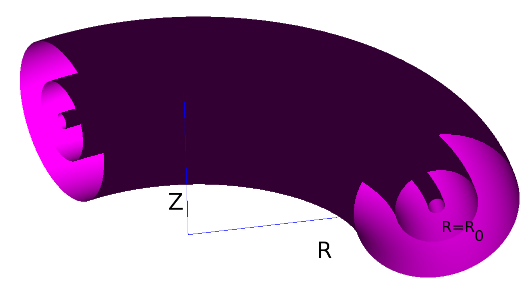
Figure 1: Cutaway diagram of a torus, showing three different flux surfaces $\varrho(\psi,s,w)$ at constant $\psi$, centred on $R=R_{0}$. (The diagram in fact shows the situation where $\psi$ is independent of $s,w$.) As explained in the text there is a correspondence between the coordinates $\psi$, $s$, $w$ and $r$, $\theta$, $\phi$ respectively. In a vertical plane, distance from the minor axis $R=R_{0}$ is usually denoted by $r$ and the poloidal angle, usually denoted by $\theta$, is measured around the minor axis. The toroidal angle, usually denoted $\phi$ is measured around the major axis $R=0$.

Further to explore the implications of this, introduce generalised toroidal coordinates $(\psi,s,w)$ (cf. $(r,\theta,\phi)$ as commonly employed in plasma physics dhaeseleer ) so that

$${\bf x}=(x,y,z)=\left(R_{+}\cos w,R_{+}\sin w,\varrho\sin s\right),$$ (97)

where

$$R_{+}=R_{0}+\varrho(\psi,s,w)\cos s$$ (98)

It will be seen from Figure 1 that $\varrho(\psi,s,w)$ at constant $\psi$ form a set of nested toroidal surfaces each having a major axis of $R_{0}$. Introduce helical coordinates $(u,v)$ on each surface, so that $s=u-v/q(\psi)$, $w=v+u/q(\psi)$, and write $\tilde{\varrho}(\psi,u,v)=\varrho(\psi,s,w)$. Suppose that $\psi$ is rotationally symmetric about the $z$-axis and satisfies the Grad-(Schlüter)-Shafranov equation (dhaeseleer, , § 8), ie. $\psi$ is a flux function for an equilibrium magnetic field, then the curves of Eq. (97) as $v$ varies at constant $u$ and $\psi$ are equivalent to lines of the equilibrium field with helical pitch $q(\psi)$. (Note that $s$ and $w$, hence $u$ and $v$ need only be suitably periodic functions of the regular toroidal angles $\theta$ and $\phi$. To define an equilibrium fully requires defining these functions, but this is inessential for what follows.) Since the metric tensor in a coordinate system $(\bar{x}^{1},\bar{x}^{2},\bar{x}^{3})$ may be written

$$g_{ik}=\frac{\partial{\bf x}}{\partial\bar{x}^{i}}\cdot\frac{\partial{\bf x}}{\partial\bar{x}^{k}}$$ (99)

taking $(\bar{x}^{1},\bar{x}^{2},\bar{x}^{3})=(\psi,u,v)$ and using suffix $i$ to denote differentiation with respect to $\bar{x}^{i}$, the components of $g_{ik}$ are straightforwardly calculated as

$$\left(\begin{matrix}R_{+}^{2}w_{\psi}^{2}+\varrho^{2}s_{\psi}^{2}+(\tilde{\varrho}_{\psi})^{2}&R_{+}^{2}w_{\psi}w_{u}+\varrho^{2}s_{\psi}s_{u}+\tilde{\varrho}_{\psi}\tilde{\varrho}_{u}&R_{+}^{2}w_{\psi}w_{v}+\varrho^{2}s_{\psi}s_{v}+\tilde{\varrho}_{\psi}\tilde{\varrho}_{v}\\ \cdot&R_{+}^{2}w_{u}^{2}+\varrho^{2}s_{u}^{2}+(\tilde{\varrho}_{u})^{2}&R_{+}^{2}w_{u}w_{v}+\varrho^{2}s_{u}s_{v}+\tilde{\varrho}_{u}\tilde{\varrho}_{v}\\ \cdot&\cdot&R_{+}^{2}w_{v}^{2}+\varrho^{2}s_{v}^{2}+(\tilde{\varrho}_{v})^{2}\\ \end{matrix}\right)$$ (100)

where the ‘dotted’ entries may be deduced from the symmetry of $g_{ik}$. The usual rules for partial differentiation give

$$\tilde{\varrho}_{\psi} = \varrho_{\psi}+\varrho_{s}s_{\psi}+\varrho_{w}w_{\psi}$$

$$\tilde{\varrho}_{u} = \varrho_{s}s_{u}+\varrho_{w}w_{u}$$ (101)

$$\tilde{\varrho}_{v} = \varrho_{s}s_{v}+\varrho_{w}w_{v}$$

The assumption of axisymmetric equilibrium is equivalent to $\varrho_{w}=0$, then substituting Eq. (101) in Eq. (100), using the Reduce-algebra system He05Redu gives

$$\left(\begin{matrix}R_{+}^{2}w_{\psi}^{2}+\varrho_{\psi}^{2}+2\varrho_{\psi}\varrho_{s}s_{\psi}+\varrho_{+}^{2}s_{\psi}^{2}&\iota R_{+}^{2}w_{\psi}+\varrho_{\psi}\varrho_{s}+\varrho_{+}^{2}s_{\psi}&-\iota\varrho_{\psi}\varrho_{s}-\iota\varrho_{+}^{2}s_{\psi}+R_{+}^{2}w_{\psi}\\ \cdot&\iota^{2}R_{+}^{2}+\varrho_{+}^{2}&\iota(R_{+}^{2}-\varrho_{+}^{2})\\ \cdot&\cdot&\iota^{2}\varrho_{+}^{2}+R_{+}^{2}\\ \end{matrix}\right)$$ (102)

where $\varrho_{+}^{2}=\varrho^{2}+\varrho_{s}^{2}$ and $\iota=1/q$ has been introduced so that $s_{i}=(s_{\psi},1,-\iota)$, $w_{i}=(w_{\psi},\iota,1)$.

This $\bar{x}^{k}$ coordinate system has been chosen so that the equilibrium field expected in the tokamak confinement device may be expressed as $\tilde{B}^{3}=1$ ($\tilde{B}^{1}=\tilde{B}^{2}=0$), but it will be seen that from the definition of $R_{+}$ in Eq. (98), the metric tensor does depend on $\bar{x}^{3}=v$ through $s=u-v\iota$. By inspection, however, in the limit when $q$ is large and constant or equivalently $\iota$ is negligible and constant (so $s_{\psi}=w_{\psi}=0$), the metric tensor becomes

$$\left(\begin{matrix}\varrho_{\psi}^{2}&\varrho_{\psi}\varrho_{s}&-\iota\varrho_{\psi}\varrho_{s}\\ \cdot&\iota^{2}R_{+}^{2}+\varrho_{+}^{2}&\iota(R_{+}^{2}-\varrho_{+}^{2})\\ \cdot&\cdot&\iota^{2}\varrho_{+}^{2}+R_{+}^{2}\\ \end{matrix}\right)$$ (103)

thus $g_{ik}$ depends only on $\bar{x}^{1}$ and $\bar{x}^{2}$. Hence a purely toroidal field, ie. one tangent to circles about the major axis $x=y=0$ of the torus, allows for flux-compression solutions. Further, when $\varrho/R_{0}$ and $\varrho_{s}$ are both small, the $s$-dependence of $g_{ik}$ is weak, so a helical field in a circular torus with relatively large major radius is also in this category. The preceding limits illustrate two of the Killing vector solution symmetries (schindler, , § 5.2.4), whereas the third is simply invariance in a Cartesian coordinate.

Lastly, if the coordinates $s$ is redefined so that $s=u$, then the metric tensor becomes

$$\left(\begin{matrix}(\varrho_{\psi}+\varrho_{s}s_{\psi})^{2}+\varrho^{2}s_{\psi}^{2}+R_{+}^{2}w_{\psi}^{2}&\iota R_{+}^{2}w_{\psi}+\varrho_{\psi}\varrho_{s}+\varrho_{+}^{2}s_{\psi}&R_{+}^{2}w_{\psi}\\ \cdot&\iota^{2}R_{+}^{2}+\varrho_{+}^{2}&\iota R_{+}^{2}\\ \cdot&\cdot&R_{+}^{2}\\ \end{matrix}\right)$$ (104)

and $g_{ik}$ depends only on $\bar{x}^{1}$ and $\bar{x}^{2}$ regardless of the presence of magnetic shear. In this coordinate system, however, lack of orthogonality makes it impossible in general to arrange so that simultaneously $\tilde{B}^{1}=\tilde{B}^{2}=0$ and $\tilde{B}^{3}=1$.

VII Summary

Section II has collated relevant results from differential geometry, especially those concerning Lie derivatives, from a widespread mathematical literature. Section III and Section IV then draw on these results to derive solutions and solution methods for the ideal MHD equations which are hopefully complementary to those presented in ref dhaeseleer , rather than simply ‘express old results in new language’. The novelty of the Lie derivative approach is that coordinate basis vector fields automatically cause the nonlinear terms in MHD to disappear. The main bar to finding solutions is then the need to satisfy the curl or ‘constitutive’ relations ${\bf J}=\nabla\times{\bf B}$ and $\mbox{\boldmath$\omega$}=\nabla\times{\bf u}$.

In kinematic, compressible MHD, where these constraints are not present, complete solution is possible (see Section VI.2), although this result was already known from the Lagrangian approach. Suggestions are made for numerical solution of the curl equations in Section III and Section IV, but it seems that for determining MHD equilibria, the Grad-Shafranov equation still has the advantage in most practical cases.

One possible practical improvement may result from the use of coordinate bases, which simplify the calculation of Lie derivatives, albeit in the example of Section III.4 at the expense of introducing non-orthogonality. Linear stability analysis to investigate this contention are outside the scope of the present work.

The reformulated equations at first sight appear to have significant coordinate invariance properties, although Section IV.3.3 shows that these are heavily qualified. The remaining parts of the present work extend ref Wa13a by (i) considering additional physics effects and how they might be modelled in the context of differential geometry (Section V), and (ii) presenting application of the flux-compression solution found in Wa13a (Section VI.3).

The current study has sought to apply results from 21st Century work on differential geometry to MHD. The mathematical notations and concepts employed in the differential geometry literature have developed significantly over the years. They may now seem to many excessively abstract, probably because the subject has been strongly driven by Quantum Mechanics and General Relativity applications, which require four or more dimensions, and by other partial differential equation applications which require infinite dimension. In 3-D, the coordinate-free approach can in fact be unhelpful. The two curl equations exemplify this, for in the newer language $\mbox{\boldmath$\omega$}=\nabla\times{\bf u}$ defines a 2-form in terms of a differential of a 1-form or vector and is written $\omega=du$. However in ${\bf J}=\nabla\times{\bf B}$, ${\bf B}$ is already a 2-form, and so its dual has to be taken before the ‘d’ operator is applied, hence is written $J=*d*B$. Since this is often accompanied by a feeling of a degree of uncertainty as to whether the operator on $B$ should be thought of acting in 3-D space or the 4-D Minkowski space-time where Maxwell’s equations are properly defined, the fact that there is no indication above that the two curl equations have the same component form, leads many to conclude that the more abstract approach just makes a hard subject even harder.

It must however be pointed out that aspects of the modern, coordinate-free approach are very valuable, for by having produced a more fundamental understanding of the subject, it indicates in what circumstances analysis might lead to physically useful results. The concept of the pull-back mapping (even if it is misleadingly named, and although not used herein) is also very useful for indicating in the presence of coordinate mappings, precisely what functions of which set of coordinates are being used. Without these latter positives, the current paper would have been much weaker and more confused.

References

- (1) W. Arter. Potential Vorticity Formulation of Compressible Magnetohydrodynamics. Physical Review Letters, 110(1):015004, 2013. DOI:10.1103/PhysRevLett.110.015004.
- (2) W.D. D’haeseleer, W.N.G. Hitchon, J.D. Callen, and J.L. Shohet. Flux Coordinates and Magnetic Structure. Springer, 1991.
- (3) K. Schindler. Physics of space plasma activity. Cambridge University Press, 2007.
- (4) V.I. Arnol’d and B.A. Khesin. Topological methods in hydrodynamics. Springer, 1998.
- (5) M.L. Woolley. On the mathematical structure of the equations of magnetohydrodynamic equilibrium. Journal of Physics A: Mathematical and General, 23(12):2379, 1990.
- (6) O.I. Bogoyavlenskij. Infinite symmetries of the ideal MHD equilibrium equations. Physics Letters A, 291(4):256–264, 2001.
- (7) O.I. Bogoyavlenskij. Symmetry transforms for ideal magnetohydrodynamics equilibria. Physical Review E, 66(5):056410, 2002.
- (8) A.F. Cheviakov. Construction of exact plasma equilibrium solutions with different geometries. Physical Review Letters, 94:165001, 2005.
- (9) G.W. Bluman, A.F. Cheviakov, and S.C. Anco. Applications of symmetry methods to partial differential equations. Springer, 2010.
- (10) M. Fecko. Differential geometry and Lie groups for physicists. Cambridge University Press, 2006.
- (11) J.F. Thompson, B. Soni, and N. Weatherill, editors. Handbook of Grid Generation. CRC Press, 1999.
- (12) D. Lovelock and H. Rund. Tensors, Differential Forms and Variational Principles. Dover, New York, 1988.
- (13) P.H. Roberts. An Introduction to Magnetohydrodynamics. Longmans, London, 1967.
- (14) R.D. Hazeltine and J.D. Meiss. Plasma Confinement. Addison-Wesley, Redwood City, 1992.
- (15) J.P. Goedbloed, R. Keppens, and S. Poedts. Advanced magnetohydrodynamics: with applications to laboratory and astrophysical plasmas. CUP, 2010.
- (16) D. MacTaggart. Finite deformation in ideal magnetohydrodynamics. Astronomy and Astrophysics, 542:A97, 2012.
- (17) W. Arter. An Anti-Perfect Dynamo Result. Physics Letters (submitted), 2013.
- (18) A.C. Hearn. Reduce: The first forty years. In Dolzmann, A. and Seidl, A. and Sturm, T., editor, Algorithmic Algebra and Logic. Proceedings of the A3L, pages 19–24. Books on Demand, Norderstedt, 2005.