Numerical evaluation of the three-point scalar-tensor cross-correlations and the tensor bi-spectrum

Abstract

Utilizing the Maldacena formalism and extending the earlier efforts to compute the scalar bi-spectrum, we construct a numerical procedure to evaluate the three-point scalar-tensor cross-correlations as well as the tensor bi-spectrum in single field inflationary models involving the canonical scalar field. We illustrate the accuracy of the adopted procedure by comparing the numerical results with the analytical results that can be obtained in the simpler cases of power law and slow roll inflation. We also carry out such a comparison in the case of the Starobinsky model described by a linear potential with a sudden change in the slope, which provides a non-trivial and interesting (but, nevertheless, analytically tractable) scenario involving a brief period of deviation from slow roll. We then utilize the code we have developed to evaluate the three-point correlation functions of interest (and the corresponding non-Gaussianity parameters that we introduce) for an arbitrary triangular configuration of the wavenumbers in three different classes of inflationary models which lead to features in the scalar power spectrum, as have been recently considered by the Planck team. We also discuss the contributions to the three-point functions during preheating in inflationary models with a quadratic minimum. We conclude with a summary of the main results we have obtained.

1 Introduction

The inflationary paradigm has now become a corner stone in our understanding of the universe at the large scales (see any of the following texts Refs. [1] or the reviews Refs. [2]). Inflation was originally introduced to overcome the so-called horizon problem of the conventional hot big bang model. Currently though, the most attractive aspect of the inflationary scenario rests on its ability to provide a mechanism for the origin of perturbations in the early universe. The perturbations generated during inflation evolve and leave their imprints as anisotropies in the Cosmic Microwave Background (CMB). With the anisotropies in the CMB being measured with constantly improving precision over the last decade or two, there have been emerging stronger and stronger constraints on the inflationary models.

Until not so long ago, constraints on inflationary models were largely arrived at by essentially comparing the models with the data at the level of the power spectrum. A nearly scale invariant primordial power spectrum, as is generated by the simplest of inflationary models, such as those involving a single scalar field and leading to a sufficiently long period of slow roll, is found to be strikingly consistent with the observations of the CMB anisotropies by the missions such as the Wilkinson Microwave Anisotropy Probe (WMAP) [3, 4, 5] and Planck [6, 7, 8] as well as various other cosmological data. However, over the last decade, it was increasingly recognized that non-Gaussianities can play a vital role in arriving at tighter constraints on models of the early universe. This expectation has been corroborated by the observations of the recent Planck mission, which has pointed to the fact that the non-Gaussianities are consistent with zero. Specifically, Planck finds that the three parameters that are often used to characterize the scalar bi-spectrum to be: $f_{{}_{\rm NL}}^{\rm loc}=2.7\pm 5.8$, $f_{{}_{\rm NL}}^{\rm eq}=-42\pm 75$ and $f_{{}_{\rm NL}}^{\rm ortho}=-25\pm 39$ [9]. These observations seem to imply that the data strongly favor slow roll inflationary models driven by a single, canonical scalar field (in this context, see the following rather comprehensive effort of comparing various models with the recent data: Ref. [10].)

Most of the efforts towards understanding non-Gaussianities generated by the inflationary models and arriving at constraints from the observational data have focused on the scalar bi-spectrum and the corresponding non-Gaussianity parameter $f_{{}_{\rm NL}}$ (for the theoretical efforts, see, for instance, Refs. [11, 12, 13]; for earlier work, i.e. prior to Planck, towards arriving at observational constraints, see, for example, Refs. [14, 15]). There have also been some theoretical efforts aimed at analyzing the behavior of the tensor bi-spectrum (see, for example, Refs. [11, 16]). But, we find that, there have been relatively limited attempts at studying the scalar-tensor cross-correlations (see, for instance, Refs. [11, 17, 18]). It will be interesting to closely examine the behavior of these quantities and, eventually, try to arrive at observational constraints on the corresponding non-Gaussianity parameters that can be constructed to characterize these quantities. The fact that tensors remain to be detected at the level of the power spectrum could have been a dissuading factor in the limited attention devoted to the cross-correlations and the tensor bi-spectrum. However, it is important to bear in mind that, popular models, such as those described by the quadratic and quartic potentials involving the canonical scalar field, are being ruled out by the Planck data primarily by the upper limits on the tensor-to-scalar ratio [8, 10]. We believe that the three-point functions involving the scalars and the tensors can play a similar role leading to additional constraints on the inflationary models.

While, as we mentioned above, a scale independent power spectrum is rather consistent with the data, certain features in the power spectrum seem to improve the fit to the data, often, at the cost of some additional parameters. For instance, features such as either a sharp cut-off at large scales [19, 20], a burst of oscillations over an intermediate range of scales [21, 22, 23] or repeated modulations extending over a wide range of scales [24, 25, 26, 27, 28, 29, 30] were known to lead to a better fit to the WMAP data than the more conventional, nearly, scale invariant, power law, primordial spectrum. Interestingly, exactly these classes of scenarios were analyzed by the Planck team, who find that, at the level of the power spectrum, while such features do improve the fit to the data, the corresponding Bayesian evidence [31] does not exhibit any substantial change [8]. Moreover, it is well established that these features can be generated only due to deviations from slow roll [32, 33, 34] (unless one assumes that the perturbations are in an excited state above the Bunch-Davies vacuum [35, 36]) which, in turn, can boost the extent of non-Gaussianities (in this context, see Refs. [37, 38, 39]), possibly, beyond the levels constrained by Planck [9]. Nevertheless, we believe that it is worthwhile examining the non-trivial scenarios further, as such exercises can aid us judge the extent of the constraints imposed by the Planck data.

In the above backdrop, the aims of this work can be said to be three fold. Firstly, extending the recent effort towards computing the scalar bi-spectrum [39], we devise a similar numerical procedure to evaluate the three-point scalar-tensor cross-correlations and the tensor bi-spectrum as well as the corresponding non-Gaussianity parameters that we introduce. Secondly, utilizing the developed numerical procedure, we evaluate these quantities in the models leading to features in the scalar power spectrum, which do not permit analytical calculation of these quantities. Thirdly, we consider the contribution to these quantities during the period of preheating, viz. the epoch which immediately follows inflation [40, 41].

The plan of this paper is as follows. In the next section, we shall begin by sketching a few essential points concerning the Maldacena formalism to arrive at the action governing the perturbations at the cubic order in inflationary scenarios involving a single canonical scalar field [11]. As should be evident, when the scalars as well as the tensors are taken into account, at the cubic order, the action can consist of either purely three scalars or tensors or it can contain cross-terms comprising of two scalars and a tensor or one scalar and two tensors. We shall describe the three-point scalar-tensor cross-correlations and the tensor bi-spectrum that these actions lead to and also discuss the corresponding non-Gaussianity parameters. In Sec. 3, we shall outline the numerical procedure that we adopt for evaluating the scalar-tensor cross-correlations and the tensor bi-spectrum. We shall begin by showing that, as in the case of the scalar bi-spectrum (in this context, see, for instance, Refs. [39, 42]), the super-Hubble contributions to the other three-point correlation functions too turn out to be negligible. Further, as in the pure scalar case, one needs to introduce a suitable cut-off in the sub-Hubble domain in order to deal with the continued oscillations that would otherwise arise. Under these conditions, we shall illustrate that, it proves to be sufficient to evolve the scalar and the tensor modes from sufficiently inside the Hubble radius to a suitably late time when they are well outside, and evaluate the integrals involved over this period. In order to demonstrate the accuracy of the numerical procedure, we shall compare our numerical results with the analytical results available in the cases of power law and slow roll inflation as well as in the case of the Starobinsky model [33, 43, 44]. (We should clarify here that the Starobinsky model that we are interested in is the one which involves a linear inflaton potential with a sharp change in its slope [33]. This clarification seems necessary at this stage, since another Starobinsky model, involving an extended theory of gravity [45], has drawn a lot of attention recently in the light of the Planck data [8].) In Sec. 4, we shall use the validated numerical code to study the three-point functions that arise in three types of models which involve deviations from slow roll, viz. the punctuated inflationary scenario [20], potentials with a step [21, 22, 23] and the so-called axion monodromy model [26, 28, 29]. In Sec. 5, we consider the contributions to the cross-correlations and the tensor bi-spectrum during preheating and show that the contributions prove to be completely insignificant. We conclude the paper in Sec. 6 with a quick summary of the results we have obtained. We relegate some of the details pertaining to the evaluation of the three-point functions in the Starobinsky model to the appendix.

Let us now make a few remarks concerning our notations and conventions. We shall work with units such that $\hbar=c=1$ and assume the Planck mass to be $M_{{}_{\rm Pl}}=\left(8\,\pi\,G\right)^{-1/2}$. We shall choose the metric signature to be $(-,+,+,+)$. Greek indices will be used to denote the spacetime coordinates, while Latin indices will denote the three spatial coordinates (except for the index $k$ which would be reserved for representing the wavenumber of the perturbations). The quantities $a$ and $H$ shall denote the scale factor and the Hubble parameter of the spatially flat, Friedmann-Lemaître-Robertson-Walker (or, simply, Friedmann, hereafter) universe. At various stages, we shall use different notions of time in the Friedmann universe, viz. the cosmic time $t$, the conformal time $\eta$, or the number of e-folds $N$, as is convenient. An overdot and an overprime shall denote differentiation with respect to the cosmic and the conformal time coordinates, respectively.

2 The cubic order actions and the three-point correlation functions

In this section, we shall briefly summarize the essential aspects of the Maldacena formalism to arrive at the three-point scalar-tensor cross-correlations and the tensor bi-spectrum. We shall also introduce the corresponding non-Gaussianity parameters, which are basically dimensionless ratios of the three-point functions and the scalar and the tensor power spectra.

2.1 The actions at the cubic order

The primary aim of the Maldacena formalism is to obtain the cubic order action that governs the scalar and the tensor perturbations. The action that describes the perturbations is arrived at by using the conventional Arnowitt-Deser-Misner (ADM) formalism [46]. Then, based on the action, one arrives at the corresponding three-point functions using the standard rules of perturbative quantum field theory [11, 12, 13].

Recall that, in the ADM formalism, the spacetime metric is expressed in terms of the lapse function $N$, the shift vector $N^{i}$ and the spatial metric $h_{ij}$ as follows:

$$ds^{2}=-N^{2}\,\left({\rm d}x^{0}\right)^{2}+h_{ij}\,\left(N^{i}\,{\rm d}x^{0}+{\rm d}x^{i}\right)\,\left(N^{j}\,{\rm d}x^{0}+{\rm d}x^{j}\right),$$ (2.1)

where $x^{0}$ and $x^{i}$ denote the time and the spatial coordinates, respectively. The system of our interest is Einsteinian gravity which is sourced by a canonical and minimally coupled scalar field, viz. the inflaton $\phi$, that is described by the potential $V(\phi)$. For such a case, the action describing the complete system can be written in terms of the metric variables $N$, $N^{i}$ and $h_{ij}$ and the scalar field $\phi$ as follows [11, 12, 13, 43]:

$$S[N,N^{i},h_{ij},\phi] = \int{\rm d}x^{0}\,\int{\rm d}^{3}{\bm{x}}\,N\,\sqrt{h}\;\Biggl{\{}\frac{M_{{}_{\rm Pl}}^{2}}{2}\left[\frac{1}{N^{2}}\,\left(E_{ij}E^{ij}-E^{2}\right)+^{(3)}\!\!R\right]$$ (2.2)

$$+\biggl{[}\frac{1}{2\,N^{2}}\,\left({\partial}_{0}\phi\right)^{2}-\frac{N^{i}}{N^{2}}\;{\partial}_{0}\phi\;{\partial}_{i}\phi-\frac{1}{2}\;h^{ij}\;{\partial}_{i}\phi\;{\partial}_{j}\phi$$

$$+\,\frac{N^{i}N^{j}}{2\,N^{2}}\,{\partial}_{i}\phi\,{\partial}_{j}\phi-V(\phi)\biggr{]}\biggr{\}},$$

where ${\partial}_{0}\phi=({\partial}\phi/{\partial}x^{0})$, $h\equiv{\rm det}~{}(h_{ij})$ and ${}^{(3)}\!R$ is the spatial curvature associated with the metric $h_{ij}$. The quantity $E_{ij}$ is given by

$$E_{ij}=\frac{1}{2}\,\left({\partial}_{0}h_{ij}-\nabla_{i}N_{j}-\nabla_{j}N_{i}\right),$$ (2.3)

with $E=h_{ij}\,E^{ij}$. As is well known, the variation of the action (2.2) with respect to the Lagrange multipliers $N$ and $N^{i}$ leads to the so-called Hamiltonian and momentum constraints, respectively. Solving these constraint equations and substituting the solutions back in the original action (2.2) permits one to arrive at the action governing the dynamical variables of interest.

As we have mentioned, our aim is to evaluate the action describing the scalar and the tensor perturbations in the spatially flat, Friedmann universe. In the absence of the perturbations, the Friedmann universe is described by the line-element

$${\rm d}s^{2}=-{\rm d}t^{2}+a^{2}(t)\,{\rm d}\bm{x}^{2},$$ (2.4)

where $\bm{x}$ represents the spatial coordinates. When the scalar and the tensor perturbations to the Friedmann metric are taken into account, it proves to be convenient to work in a specific gauge to arrive at the action governing the perturbations. As is often done in this context, we shall choose to work in the so-called co-moving gauge [11]. In such a gauge, the perturbation in the scalar field is assumed to be absent, so that the quantity $\phi$ that appears in the action (2.2) actually depends only on time. Moreover, the three metric $h_{ij}$ is written as

$$h_{ij}=a^{2}(t)\;{\rm e}^{2\,{\cal R}(t,\bm{x})}\,\left[{\rm e}^{\gamma(t,\bm{x})}\right]_{ij},$$ (2.5)

where ${\mathcal{R}}$ denotes the curvature perturbation describing the scalars, while $\gamma_{ij}$ represents the transverse and traceless (i.e. $\partial_{j}\gamma_{ij}=\gamma_{ii}=0$) tensor perturbations. These assumptions for the scalar field $\phi$ and the spatial metric $h_{ij}$ as well as the solutions to the constraint equations then allows one to arrive at the action describing the perturbations, viz. the quantities ${\mathcal{R}}$ and $\gamma_{ij}$, at a given order [11, 12]. The action at the quadratic order leads to the linear equations of motion governing the perturbations. In Fourier space, the scalar and the tensor modes satisfy the differential equations

$${\mathcal{R}}_{\bm{k}}^{\prime\prime}+2\,\frac{z^{\prime}}{z}\,{\mathcal{R}}_{\bm{k}}^{\prime}+k^{2}\,{\mathcal{R}}_{\bm{k}} = 0,$$ (2.6a)

$$\gamma_{\bm{k}}^{\prime\prime}+2\,\frac{a^{\prime}}{a}\,\gamma_{\bm{k}}^{\prime}+k^{2}\,\gamma_{\bm{k}} = 0,$$ (2.6b)

respectively, where $z=\sqrt{2\,\epsilon_{1}}\,a\,M_{{}_{\rm Pl}}$, with $\epsilon_{1}=-{\dot{H}}/H^{2}$ being the first slow roll parameter. We should add that, when no confusion can arise, here and hereafter, we shall suppress the indices of the tensor perturbations for convenience.

In the co-moving gauge, at the cubic order in the perturbations, evidently, the action will consist of terms of the form ${\cal RRR}$, ${\cal RR}\gamma$, ${\cal R}\gamma\gamma$ and $\gamma\gamma\gamma$. The term involving ${\cal RRR}$ leads to the scalar bi-spectrum. Since we are interested only in the scalar-tensor cross-correlations and the tensor bi-spectrum, we shall focus on the actions that lead to these quantities. The actions that lead to correlations involving two scalars and one tensor, one scalar and two tensors and three tensors are given by (see, for example, Refs. [11, 16, 17])

$$S^{3}_{{\cal RR}\gamma}[{\mathcal{R}},\gamma_{ij}] = M_{{}_{\rm Pl}}^{2}\,\int{\rm d}\eta\,\int{\rm d}^{3}\bm{x}\;\biggl{[}a^{2}\,\epsilon_{1}\,\gamma_{ij}\,{\partial}_{i}{\cal R}\,{\partial}_{j}{\cal R}+\frac{1}{4}\,{\partial}^{2}\gamma_{ij}\,\partial_{i}\chi\,\partial_{j}\chi$$ (2.7a)

$$+\,\frac{a\,\epsilon_{1}}{2}\,\gamma_{ij}^{\prime}\,\partial_{i}{\cal R}\,\partial_{j}\chi+{\mathcal{F}}^{2}_{ij}({\cal R})\,\frac{\delta{\cal L}^{2}_{\gamma\gamma}}{\delta\gamma_{ij}}+{\mathcal{F}}^{3}({\mathcal{R}},\gamma_{ij})\,\frac{\delta{\cal L}^{2}_{{\mathcal{R}}{\mathcal{R}}}}{\delta{\cal R}}\biggr{]},$$

$$S^{3}_{{\cal R}\gamma\gamma}[{\mathcal{R}},\gamma_{ij}] = \frac{M_{{}_{\rm Pl}}^{2}}{4}\,\int{\rm d}\eta\,\int{\rm d}^{3}\bm{x}\;\biggl{[}\frac{a^{2}\,\epsilon_{1}}{2}\,{\cal R}\,\gamma_{ij}^{\prime}\,\gamma_{ij}^{\prime}+\frac{a^{2}\,\epsilon_{1}}{2}\,{\cal R}\,{\partial}_{l}\gamma_{ij}\,{\partial}_{l}\gamma_{ij}$$ (2.7b)

$$-\,a\,\gamma_{ij}^{\prime}\,{\partial}_{l}\gamma_{ij}\,{\partial}_{l}\chi+{\mathcal{F}}^{4}_{ij}({\mathcal{R}},\gamma_{mn})\,\frac{\delta{\cal L}^{2}_{\gamma\gamma}}{\delta\gamma_{ij}}\biggr{]},$$

$$S^{3}_{\gamma\gamma\gamma}[\gamma_{ij}] = \frac{M_{{}_{\rm Pl}}^{2}}{2}\,\int{\rm d}\eta\,\int{\rm d}^{3}\bm{x}\;\biggl{[}\frac{a^{2}}{2}\,\gamma_{lj}\,\gamma_{im}\,{\partial}_{l}{\partial}_{m}\gamma_{ij}-\,\frac{a^{2}}{4}\,\gamma_{ij}\,\gamma_{lm}\,{\partial}_{l}{\partial}_{m}\gamma_{ij}\biggr{]}.$$ (2.7c)

In these actions, the quantity $\chi$ is determined by the relation $\partial^{2}\chi=a\,\epsilon_{1}\,{\cal R}^{\prime}$, and the quantities $\mathcal{L}^{2}_{{\cal R}{\cal R}}$ and $\mathcal{L}^{2}_{\gamma\gamma}$ are the second order Lagrangian densities comprising of two scalars and tensors which lead to the equations of motion (2.6). One can show that the terms proportional to $(\delta{\cal L}^{2}_{{\cal R}{\cal R}}/\delta{\cal R})$ and $(\delta{\cal L}^{2}_{\gamma\gamma}/\delta\gamma_{ij})$ can be removed by suitable field redefinitions (for further details, including the explicit forms of the functions ${\mathcal{F}}^{2}_{ij}({\mathcal{R}})$, ${\mathcal{F}}^{3}({\mathcal{R}},\gamma_{ij})$ and ${\mathcal{F}}^{4}_{ij}({\mathcal{R}},\gamma_{mn})$, see Refs. [11, 12, 13, 16, 17]).

In order to calculate the three-point correlation functions using the methods of quantum field theory, one requires the interaction Hamiltonian corresponding to the above actions. We note that, at the cubic order, the interaction Hamiltonian $H_{\rm int}$ is related to the interaction Lagrangian $L_{\rm int}$ through the relation: $H_{\rm int}=-L_{\rm int}$ [11, 12, 13, 16, 17]. In what follows, we shall refer to $H_{\rm int}$ corresponding to the various actions as $H_{\sf ABC}$, where each of $({\sf A},{\sf B},{\sf C})$ can be either a ${\mathcal{R}}$ or a $\gamma$. In the next sub-section, we shall make use of the above actions (actually, the corresponding interaction Hamiltonians) to compute the three-point functions of our interest.

2.2 The three-point functions of interest and the different contributions

Given the interaction Hamiltonian, the corresponding three-point function can be evaluated using the standard rules of perturbative quantum field theory. The three-point functions can be expressed in terms of products of operators which satisfy the linear equations of motion. In the cases of our interest, the quantum operators associated with the classical variables, viz. the curvature perturbation ${\mathcal{R}}$ and the tensor perturbation $\gamma_{ij}$, can be decomposed in terms of the corresponding Fourier modes as follows [1, 2]:

$$\hat{{\mathcal{R}}}(\eta,{\bf x}) = \int\frac{{\rm d}^{3}{\bm{k}}}{\left(2\,\pi\right)^{3/2}}\,\hat{{\mathcal{R}}}_{\bm{k}}(\eta)\,{\rm e}^{i\,{\bm{k}}\cdot{\bm{x}}}$$ (2.8a)

$$= \int\frac{{\rm d}^{3}{\bm{k}}}{\left(2\,\pi\right)^{3/2}}\,\left(\hat{a}_{\bm{k}}\,f_{k}(\eta)\,{\rm e}^{i\,{\bm{k}}\cdot{\bm{x}}}+\hat{a}^{\dagger}_{\bf k}\,f^{*}_{k}(\eta)\,{\rm e}^{-i\,{\bm{k}}\cdot{\bm{x}}}\right),$$

$$\hat{\gamma}_{ij}(\eta,{\bf x}) = \int\frac{{\rm d}^{3}{\bm{k}}}{\left(2\,\pi\right)^{3/2}}\,\hat{\gamma}_{ij}^{\bm{k}}(\eta)\,{\rm e}^{i\,{\bm{k}}\cdot{\bm{x}}}$$ (2.8b)

$$= \sum_{s}\int\frac{{\rm d}^{3}{\bm{k}}}{(2\,\pi)^{3/2}}\,\left(\hat{b}^{s}_{\bm{k}}\,\varepsilon^{s}_{ij}({\bm{k}})\,g_{k}(\eta)\,{\rm e}^{i\,{\bm{k}}\cdot{\bm{x}}}+\hat{b}^{s\dagger}_{\bf k}\,\varepsilon^{s*}_{ij}({\bm{k}})\,g^{*}_{k}(\eta)\,{\rm e}^{-i\,{\bm{k}}\cdot{\bm{x}}}\right),$$

where the scalar and tensor modes $f_{k}$ and $g_{k}$ satisfy the equations of motion (2.6). The quantity $\varepsilon^{s}_{ij}({\bm{k}})$ represents the polarization tensor of the gravitational waves, with the index $s$ denoting the helicity of the graviton. In the gauge we are working in, the polarization tensor obeys the relations $\varepsilon^{s}_{ii}({\bm{k}})=k_{i}\,\varepsilon_{ij}^{s}({\bm{k}})=0$, and we choose to work with the normalization: $\varepsilon_{ij}^{r}({\bm{k}})\,\varepsilon_{ij}^{s}({\bm{k}})=2\,\delta^{rs}$ [11]. In the above equations, the pairs of operators $(\hat{a}_{\bm{k}},\hat{a}^{\dagger}_{\bm{k}})$ and $(\hat{b}_{\bm{k}}^{s},\hat{b}^{s\dagger}_{\bm{k}})$ denote the annihilation and creation operators corresponding to the scalar and the tensor modes associated with the wavevector ${\bm{k}}$. They obey the following non-trivial commutation relations: $[\hat{a}_{\bm{k}},\hat{a}^{\dagger}_{\bm{k}^{\prime}}]=\delta^{(3)}({\bm{k}}-{\bm{k}}^{\prime})$ and $[\hat{b}^{r}_{\bm{k}},\hat{b}_{\bm{k}^{\prime}}^{s\dagger}]=\delta^{(3)}({\bm{k}}-{\bm{k}}^{\prime})\,\delta^{rs}$.

It should be mentioned here that the scalar and the tensor power spectra, viz. ${\mathcal{P}}_{{}_{\rm S}}(k)$ and ${\mathcal{P}}_{{}_{\rm T}}(k)$, are defined as follows:

$$\langle 0|{\hat{\mathcal{R}}}_{\bm{k}}(\eta)\,{\hat{\mathcal{R}}}_{\bm{k}^{\prime}}(\eta)|0\rangle = \frac{(2\,\pi)^{2}}{2\,k^{3}}\,{\mathcal{P}}_{{}_{\rm S}}(k)\;\delta^{(3)}({\bm{k}}+{\bm{k}^{\prime}}),$$ (2.9a)

$$\langle 0|{\hat{\gamma}}_{ij}^{\bm{k}}(\eta)\,{\hat{\gamma}}_{ij}^{\bm{k}^{\prime}}(\eta)|0\rangle = \frac{(2\,\pi)^{2}}{2\,k^{3}}\,{\mathcal{P}}_{{}_{\rm T}}(k)\;\delta^{(3)}({\bm{k}}+{\bm{k}^{\prime}}),$$ (2.9b)

where the vacuum state $|0\rangle$ is defined as ${\hat{a}}_{\bm{k}}|0\rangle=0$ and ${\hat{b}}_{\bm{k}}^{s}|0\rangle=0$ for all ${\bm{k}}$ and $s$. Upon using the decompositions (2.8), the power spectra can be expressed in terms of the modes $f_{k}$ and $g_{k}$ as

$${\mathcal{P}}_{{}_{\rm S}}(k) = \frac{k^{3}}{2\,\pi^{2}}\,|f_{k}|^{2},$$ (2.10a)

$${\mathcal{P}}_{{}_{\rm T}}(k) = 4\,\frac{k^{3}}{2\,\pi^{2}}\,|g_{k}|^{2},$$ (2.10b)

with the right hand sides evaluated at late times when the amplitude of the modes have frozen when they are well outside the Hubble radius during the inflationary epoch.

2.2.1 The scalar-tensor cross-correlations

The two scalar-tensor cross-correlations in Fourier space, viz. ${\cal B}_{{\mathcal{R}}{\mathcal{R}}\gamma}^{m_{3}n_{3}}({\bm{k}}_{1},{\bm{k}}_{2},{\bm{k}}_{3})$ which involves two scalars and a tensor and ${\cal B}_{{\mathcal{R}}\gamma\gamma}^{m_{2}n_{2}m_{3}n_{3}}({\bm{k}}_{1},{\bm{k}}_{2},{\bm{k}}_{3})$ which involves one scalar and two tensors, evaluated, say, towards the end of inflation, at the conformal time $\eta_{\rm e}$, are defined as

$$\langle{\hat{\mathcal{R}}}_{{\bm{k}}_{1}}(\eta_{\rm e})\,{\hat{\mathcal{R}}}_{{\bm{k}}_{2}}(\eta_{\rm e})\,{\hat{\gamma}}_{m_{3}n_{3}}^{{\bm{k}}_{3}}(\eta_{\rm e})\,\rangle = \left(2\,\pi\right)^{3}{\cal B}_{{\cal R}{\cal R}\gamma}^{m_{3}n_{3}}({\bm{k}}_{1},{\bm{k}}_{2},{\bm{k}}_{3})\;\delta^{(3)}\left({\bm{k}}_{1}+{\bm{k}}_{2}+{\bm{k}}_{3}\right),$$ (2.11)

$$\langle{\hat{\mathcal{R}}}_{{\bm{k}}_{1}}(\eta_{\rm e})\,{\hat{\gamma}}_{m_{2}n_{2}}^{{\bm{k}}_{2}}(\eta_{\rm e})\,{\hat{\gamma}}_{m_{3}n_{3}}^{{\bm{k}}_{3}}(\eta_{\rm e})\rangle = \left(2\,\pi\right)^{3}{\cal B}_{{\cal R}\gamma\gamma}^{m_{2}n_{2}m_{3}n_{3}}({\bm{k}}_{1},{\bm{k}}_{2},{\bm{k}}_{3})\;\delta^{(3)}\left({\bm{k}}_{1}+{\bm{k}}_{2}+{\bm{k}}_{3}\right).\quad$$ (2.12)

(As we have mentioned earlier, occasionally, for ease of notation, we may drop the tensor indices such as $mn$ when they do not lead to ambiguities.) At the leading order in perturbation theory, these quantities can be expressed in terms of the corresponding interaction Hamiltonians ${\hat{H}}_{{\mathcal{R}}{\mathcal{R}}\gamma}$ and ${\hat{H}}_{{\mathcal{R}}\gamma\gamma}$ [obtained from the actions (2.7a) and (2.7b)] as follows [11]:

$$\langle{\hat{\mathcal{R}}}_{{\bm{k}}_{1}}(\eta_{\rm e})\,{\hat{\mathcal{R}}}_{{\bm{k}}_{2}}(\eta_{\rm e})\,{\hat{\gamma}}_{m_{3}n_{3}}^{{\bm{k}}_{3}}(\eta_{\rm e})\rangle = -i\,\int_{\eta_{\rm i}}^{\eta_{\rm e}}{\rm d}\eta\;\langle[{\hat{\mathcal{R}}}_{{\bm{k}}_{1}}(\eta_{\rm e})\,{\hat{\mathcal{R}}}_{{\bm{k}}_{2}}(\eta_{\rm e})\,{\hat{\gamma}}_{m_{3}n_{3}}^{{\bm{k}}_{3}}(\eta_{\rm e}),\hat{H}_{{\cal R}{\cal R}\gamma}(\eta)]\rangle,\qquad$$ (2.13)

$$\langle{\hat{\mathcal{R}}}_{{\bm{k}}_{1}}(\eta_{\rm e})\,{\hat{\gamma}}_{m_{2}n_{2}}^{{\bm{k}}_{2}}(\eta_{\rm e})\,{\hat{\gamma}}_{m_{3}n_{3}}^{{\bm{k}}_{3}}(\eta_{\rm e})\rangle = -i\,\int_{\eta_{\rm i}}^{\eta_{\rm e}}{\rm d}\eta\;\langle[{\hat{\mathcal{R}}}_{{\bm{k}}_{1}}(\eta_{\rm e})\,{\hat{\gamma}}_{m_{2}n_{2}}^{{\bm{k}}_{2}}(\eta_{\rm e})\,{\hat{\gamma}}_{m_{3}n_{3}}^{{\bm{k}}_{3}}(\eta_{\rm e}),\hat{H}_{{\cal R}\gamma\gamma}(\eta)]\rangle,\quad$$

where $\eta_{i}$ is the time when the initial conditions are imposed (when the largest mode of interest is sufficiently inside the Hubble radius during inflation), the square brackets imply the commutation of the operators, while the angular brackets denote the fact that the expectation values are to be evaluated in the initial vacuum state. For convenience, we shall set

$${\cal B}_{\sf ABC}({\bm{k}}_{1},{\bm{k}}_{2},{\bm{k}}_{3})=\left(2\,\pi\right)^{-9/2}\,G_{\sf ABC}({\bm{k}}_{1},{\bm{k}}_{2},{\bm{k}}_{3}).$$ (2.15)

Upon using the above expressions, the mode decompositions (2.8) and Wick’s theorem, which applies to Gaussian random fields, we obtain that

$$G_{{\cal R}{\cal R}\gamma}^{m_{3}n_{3}}({\bm{k}}_{1},{\bm{k}}_{2},{\bm{k}}_{3}) = \sum_{C=1}^{3}\;G_{{\cal R}{\cal R}\gamma\,(C)}^{m_{3}n_{3}}({\bm{k}}_{1},{\bm{k}}_{2},{\bm{k}}_{3})$$ (2.16)

$$= M_{{}_{\rm Pl}}^{2}\;\sum_{C=1}^{3}\,\sum_{s_{3}}\ \biggl{\{}\left[\varepsilon_{m_{3}n_{3}}^{s_{3}}({\bm{k}}_{3})\,f_{{k_{1}}}(\eta_{\rm e})\,f_{{k_{2}}}(\eta_{\rm e})\,g_{{k_{3}}}(\eta_{\rm e})\right]$$

$$\times\;{\cal G}_{{\cal R}{\cal R}\gamma}^{C}({\bm{k}}_{1},{\bm{k}}_{2},{\bm{k}}_{3})+{\rm complex~{}conjugate}\biggr{\}},$$

where the quantities ${\cal G}_{{\cal R}{\cal R}\gamma}^{C}({\bm{k}}_{1},{\bm{k}}_{2},{\bm{k}}_{3})$ are described by the integrals

$${\cal G}_{{\cal R}{\cal R}\gamma}^{1}({\bm{k}}_{1},{\bm{k}}_{2},{\bm{k}}_{3}) = -2\;i\;\varepsilon_{ij}^{s_{3}\ast}({\bm{k}}_{3})\;k_{1i}\,k_{2j}\,\int_{\eta_{\rm i}}^{\eta_{\rm e}}{\rm d}\eta\;a^{2}\,\epsilon_{1}\,f_{{k_{1}}}^{\ast}\,f_{{k_{2}}}^{\ast}\,g_{{k_{3}}}^{\ast},$$ (2.17a)

$${\cal G}_{{\cal R}{\cal R}\gamma}^{2}({\bm{k}}_{1},{\bm{k}}_{2},{\bm{k}}_{3}) = \frac{i}{2}\;\varepsilon_{ij}^{s_{3}\ast}({\bm{k}}_{3})\;\frac{k_{1i}\,k_{2j}\,k_{3}^{2}}{k_{1}^{2}\,k_{2}^{2}}\,\int_{\eta_{\rm i}}^{\eta_{\rm e}}{\rm d}\eta\;a^{2}\,\epsilon_{1}^{2}\,f_{{k_{1}}}^{\prime\ast}\,f_{{k_{2}}}^{\prime\ast}\,g_{{k_{3}}}^{\ast},$$ (2.17b)

$${\cal G}_{{\cal R}{\cal R}\gamma}^{3}({\bm{k}}_{1},{\bm{k}}_{2},{\bm{k}}_{3}) = \frac{i}{2}\,\varepsilon_{ij}^{s_{3}\ast}({\bm{k}}_{3})\,\frac{k_{1i}\,k_{2j}}{k_{1}^{2}\,k_{2}^{2}}\,\int_{\eta_{\rm i}}^{\eta_{\rm e}}{\rm d}\eta\;a^{2}\,\epsilon_{1}^{2}\,\left[k_{1}^{2}\,f_{{k_{1}}}^{\ast}\,f_{{k_{2}}}^{\prime\ast}+k_{2}^{2}\,f_{{k_{1}}}^{\prime\ast}\,f_{{k_{2}}}^{\ast}\right]\,g_{{k_{3}}}^{\prime\ast},\quad$$ (2.17c)

which, evidently, correspond to the three different terms that constitute the action $S_{{\mathcal{R}}{\mathcal{R}}\gamma}$ [cf. Eq. (2.7a)]. It is worth mentioning here that, while the first term is of the order of the first slow roll parameter $\epsilon_{1}$, the remaining two terms are of the order $\epsilon_{1}^{2}$ [11]. In exactly the same way, we can obtain that

$$G_{{\cal R}\gamma\gamma}^{m_{2}n_{2}m_{3}n_{3}}({\bm{k}}_{1},{\bm{k}}_{2},{\bm{k}}_{3}) = \sum_{C=1}^{3}\;G_{{\cal R}\gamma\gamma\,(C)}^{m_{2}n_{2}m_{3}n_{3}}({\bm{k}}_{1},{\bm{k}}_{2},{\bm{k}}_{3})$$ (2.18)

$$= M_{{}_{\rm Pl}}^{2}\;\sum_{C=1}^{3}\;\sum_{s_{2},s_{3}}\,\Biggl{\{}\left[\varepsilon_{m_{2}n_{2}}^{s_{2}}({\bm{k}}_{2})\,\varepsilon_{m_{3}n_{3}}^{s_{3}}({\bm{k}}_{3})\,f_{{k_{1}}}(\eta_{\rm e})\,g_{{k_{2}}}(\eta_{\rm e})\,g_{{k_{3}}}(\eta_{\rm e})\right]$$

$$\times\;{\cal G}_{{\cal R}\gamma\gamma}^{C}({\bm{k}}_{1},{\bm{k}}_{2},{\bm{k}}_{3})+{\rm complex~{}conjugate}\Biggr{\}},$$

with the quantities ${\cal G}_{{\cal R}\gamma\gamma}^{C}({\bm{k}}_{1},{\bm{k}}_{2},{\bm{k}}_{3})$ being given by

$${\cal G}_{{\cal R}\gamma\gamma}^{1}({\bm{k}}_{1},{\bm{k}}_{2},{\bm{k}}_{3}) = \frac{i}{4}\;\varepsilon_{ij}^{s_{2}\ast}({\bm{k}}_{2})\;\varepsilon_{ij}^{s_{3}\ast}({\bm{k}}_{3})\;\int_{\eta_{\rm i}}^{\eta_{\rm e}}{\rm d}\eta\;a^{2}\,\epsilon_{1}\,f_{{k_{1}}}^{\ast}\,g_{{k_{2}}}^{\prime\ast}\,g_{{k_{3}}}^{\prime\ast},$$ (2.19a)

$${\cal G}_{{\cal R}\gamma\gamma}^{2}({\bm{k}}_{1},{\bm{k}}_{2},{\bm{k}}_{3}) = -\frac{i}{4}\;\varepsilon_{ij}^{s_{2}\ast}({\bm{k}}_{2})\;\varepsilon_{ij}^{s_{3}\ast}({\bm{k}}_{3})\;\left({\bm{k}}_{2}\cdot{\bm{k}}_{3}\right)\,\int_{\eta_{\rm i}}^{\eta_{\rm e}}{\rm d}\eta\;a^{2}\,\epsilon_{1}\,f_{{k_{1}}}^{\ast}\,g_{{k_{2}}}^{\ast}\,g_{{k_{3}}}^{\ast},$$ (2.19b)

$${\cal G}_{{\cal R}\gamma\gamma}^{3}({\bm{k}}_{1},{\bm{k}}_{2},{\bm{k}}_{3}) = -\frac{i}{4}\;\varepsilon_{ij}^{s_{2}\ast}({\bm{k}}_{2})\;\varepsilon_{ij}^{s_{3}\ast}({\bm{k}}_{3})\;\int_{\eta_{\rm i}}^{\eta_{\rm e}}{\rm d}\eta\;a^{2}\,\epsilon_{1}\,f_{{k_{1}}}^{\prime\ast}\,\biggl{[}\frac{{\bm{k}}_{1}\cdot{\bm{k}}_{3}}{k_{1}^{2}}\,\,g_{{k_{2}}}^{\prime\ast}\,g_{{k_{3}}}^{\ast}$$ (2.19c)

$$+\,\frac{{\bm{k}}_{1}\cdot{\bm{k}}_{2}}{k_{1}^{2}}\,g_{{k_{2}}}^{\ast}\,g_{{k_{3}}}^{\prime\ast}\biggr{]},$$

which, again, correspond to the three different terms in the action $S_{{\cal R}\gamma\gamma}$ [cf. Eq. (2.7b)]. Note that, in this case, all the terms are of the same order in the first slow roll parameter $\epsilon_{1}$. The hierarchy of the various contributions to the cross-correlations will also be evident when we discuss specific analytic and numerical results in the following section.

2.2.2 The tensor bi-spectrum

The tensor bi-spectrum ${\cal B}_{\gamma\gamma\gamma}^{m_{1}n_{1}m_{2}n_{2}m_{3}n_{3}}({\bm{k}}_{1},{\bm{k}}_{2},{\bm{k}}_{3})$ is defined as

$$\langle{\hat{\gamma}}_{m_{1}n_{1}}^{{\bm{k}}_{1}}(\eta_{\rm e})\,{\hat{\gamma}}_{m_{2}n_{2}}^{{\bm{k}}_{2}}(\eta_{\rm e})\,{\hat{\gamma}}_{m_{3}n_{3}}^{{\bm{k}}_{3}}(\eta_{\rm e})\rangle=\left(2\,\pi\right)^{3}{\cal B}_{\gamma\gamma\gamma}^{m_{1}n_{1}m_{2}n_{2}m_{3}n_{3}}({\bm{k}}_{1},{\bm{k}}_{2},{\bm{k}}_{3})\;\delta^{(3)}\left({\bm{k}}_{1}+{\bm{k}}_{2}+{\bm{k}}_{3}\right)$$ (2.20)

and, clearly, in terms of the Hamiltonian ${\hat{H}}_{\gamma\gamma\gamma}$, it can be expressed as

$$\langle{\hat{\gamma}}_{m_{1}n_{1}}^{{\bm{k}}_{1}}(\eta_{\rm e})\,{\hat{\gamma}}_{m_{2}n_{2}}^{{\bm{k}}_{2}}(\eta_{\rm e})\,{\hat{\gamma}}_{m_{3}n_{3}}^{{\bm{k}}_{3}}(\eta_{\rm e})\rangle=-i\,\int_{\eta_{\rm i}}^{\eta_{\rm e}}{\rm d}\eta\;\langle[{\hat{\gamma}}_{m_{1}n_{1}}^{{\bm{k}}_{1}}(\eta_{\rm e})\,{\hat{\gamma}}_{m_{2}n_{2}}^{{\bm{k}}_{2}}(\eta_{\rm e})\,{\hat{\gamma}}_{m_{3}n_{3}}^{{\bm{k}}_{3}}(\eta_{\rm e}),\hat{H}_{\gamma\gamma\gamma}(\eta)]\rangle.$$ (2.21)

The corresponding quantity $G_{\gamma\gamma\gamma}^{m_{1}n_{1}m_{2}n_{2}m_{3}n_{3}}({\bm{k}}_{1},{\bm{k}}_{2},{\bm{k}}_{3})$ can be arrived in the same fashion as the cross-correlations from the action $S_{\gamma\gamma\gamma}$ [cf. Eq. (2.7c)]. It can be written as [11, 16]

$$G_{\gamma\gamma\gamma}^{m_{1}n_{1}m_{2}n_{2}m_{3}n_{3}}({\bm{k}}_{1},{\bm{k}}_{2},{\bm{k}}_{3}) = \sum_{C=1}^{2}\;G_{\gamma\gamma\gamma\,(C)}({\bm{k}}_{1},{\bm{k}}_{2},{\bm{k}}_{3})$$ (2.22)

$$= M_{{}_{\rm Pl}}^{2}\;\sum_{C=1}^{2}\;\sum_{s_{1},s_{2},s_{3}}\Biggl{\{}\biggl{[}\varepsilon_{m_{1}n_{1}}^{s_{1}}({\bm{k}}_{1})\;\varepsilon_{m_{2}n_{2}}^{s_{2}}({\bm{k}}_{2})\;\varepsilon_{m_{3}n_{3}}^{s_{3}}({\bm{k}}_{3})$$

$$\times\;g_{{k_{1}}}(\eta_{\rm e})\,g_{{k_{2}}}(\eta_{\rm e})\,g_{{k_{3}}}(\eta_{\rm e})\biggr{]}\;{\cal G}_{\gamma\gamma\gamma}^{C}({\bm{k}}_{1},{\bm{k}}_{2},{\bm{k}}_{3})$$

$$+\,{\rm complex~{}conjugate}\Biggr{\}},$$

where the quantities ${\cal G}_{\gamma\gamma\gamma}^{C}({\bm{k}}_{1},{\bm{k}}_{2},{\bm{k}}_{3})$ are described by the integrals

$${\cal G}_{\gamma\gamma\gamma}^{1}({\bm{k}}_{1},{\bm{k}}_{2},{\bm{k}}_{3}) = -\frac{i}{4}\;\left[\varepsilon_{ij}^{s_{1}\ast}({\bm{k}}_{1})\;\varepsilon_{im}^{s_{2}\ast}({\bm{k}}_{2})\;\varepsilon_{lj}^{s_{3}\ast}({\bm{k}}_{3})\;k_{1m}\,k_{1l}+{\rm five~{}permutations}\right]$$ (2.23a)

$$\times\,\int_{\eta_{\rm i}}^{\eta_{\rm e}}{\rm d}\eta\;a^{2}\,g_{{k_{1}}}^{\ast}\,g_{{k_{2}}}^{\ast}\,g_{{k_{3}}}^{\ast},$$

$${\cal G}_{\gamma\gamma\gamma}^{2}({\bm{k}}_{1},{\bm{k}}_{2},{\bm{k}}_{3}) = \frac{i}{8}\;\left[\varepsilon_{ij}^{s_{1}\ast}({\bm{k}}_{1})\;\varepsilon_{ml}^{s_{2}\ast}({\bm{k}}_{2})\;\varepsilon_{ij}^{s_{3}\ast}({\bm{k}}_{3})\;k_{1m}\,k_{1l}+{\rm five~{}permutations}\right]$$ (2.23b)

$$\times\,\int_{\eta_{\rm i}}^{\eta_{\rm e}}{\rm d}\eta\;a^{2}\,g_{{k_{1}}}^{\ast}\,g_{{k_{2}}}^{\ast}\,g_{{k_{3}}}^{\ast}.$$

It is evident that the two contributions to the tensor bi-spectrum are of the same order in magnitude. Again, this will be corroborated by explicit analytical and numerical calculations in due course.

2.3 The non-Gaussianity parameters

Recall that, often, the scalar bi-spectrum is essentially characterized by the dimensionless non-Gaussianity parameters $f_{{}_{\rm NL}}$. The basic set of three non-Gaussianity parameters, viz. $(f_{{}_{\rm NL}}^{\rm loc},f_{{}_{\rm NL}}^{\rm eq},f_{{}_{\rm NL}}^{\rm ortho})$, do not always capture the complete structure of the scalar bi-spectrum, in particular, when there exist deviations from the conventional scenario of slow roll inflation driven by the canonical scalar field (and, of course, the assumption that the perturbations are in the standard Bunch-Davies vacuum [1, 2, 35]). Nonetheless, they prove to be a convenient tool in understanding the amplitude and shape of the scalar bi-spectrum in many situations.

In a similar manner, one can characterize the cross-correlations and the tensor bi-spectrum by parameters that are suitable dimensionless ratios of the three-point functions and the scalar or the tensor power spectra. One can generalize the conventional way of introducing the $f_{{}_{\rm NL}}$ parameter to write the scalar and tensor perturbations ${\mathcal{R}}$ and $\gamma_{ij}$ as follows:

$${\mathcal{R}}(\eta,{\bm{x}})={\mathcal{R}}^{\rm G}(\eta,{\bm{x}})-\frac{3\,f_{{}_{\rm NL}}}{5}\;[{\cal R}^{\rm G}(\eta,{\bm{x}})]^{2}-C_{{}_{\rm NL}}^{\mathcal{R}}\;{\mathcal{R}}^{\rm G}(\eta,{\bm{x}})\;\gamma_{{\bar{m}}{\bar{n}}}^{\rm G}(\eta,{\bm{x}})$$ (2.24)

and

$$\gamma_{ij}(\eta,{\bm{x}})=\gamma_{ij}^{\rm G}(\eta,{\bm{x}})-h_{{}_{\rm NL}}\;\gamma_{ij}^{\rm G}(\eta,{\bm{x}})\;\gamma_{{\bar{m}}{\bar{n}}}^{\rm G}(\eta,{\bm{x}})-C_{{}_{\rm NL}}^{\mathcal{\gamma}}\;\gamma_{ij}^{\rm G}(\eta,{\bm{x}})\;{\mathcal{R}}^{\rm G}(\eta,{\bm{x}}),$$ (2.25)

where ${\mathcal{R}}^{\rm G}$ and $\gamma_{ij}^{\rm G}$ denote the Gaussian quantities. Note that the overbars on the indices of the Gaussian tensor perturbation imply that the indices should be summed over all allowed values. Upon using the above definitions along with the Wick’s theorem to calculate the three-point functions (but, retaining terms only to the linear order in the non-Gaussianity parameters), we find that we can write the parameters $C_{{}_{\rm NL}}^{\mathcal{R}}$, $C_{{}_{\rm NL}}^{\mathcal{\gamma}}$ and $h_{{}_{\rm NL}}$ as follows:

$$C_{{}_{\rm NL}}^{\mathcal{R}} = -\frac{4}{\left(2\,\pi^{2}\right)^{2}}\,\left[k_{1}^{3}\,k_{2}^{3}\,k_{3}^{3}\;G_{{\mathcal{R}}{\mathcal{R}}\gamma}^{m_{3}n_{3}}({\bm{k}}_{1},{\bm{k}}_{2},{\bm{k}}_{3})\right]$$ (2.26)

$$\times\;{\left(\Pi_{m_{3}n_{3},{\bar{m}}{\bar{n}}}^{{\bm{k}}_{3}}\right)}^{-1}\;\,\biggl{\{}\left[k_{1}^{3}\;{\mathcal{P}}_{{}_{\rm S}}(k_{2})+k_{2}^{3}\;{\mathcal{P}}_{{}_{\rm S}}(k_{1})\right]\;{\mathcal{P}}_{{}_{\rm T}}(k_{3})\biggr{\}}^{-1},$$

$$C_{{}_{\rm NL}}^{\mathcal{\gamma}} = -\frac{4}{\left(2\,\pi^{2}\right)^{2}}\,\left[k_{1}^{3}\,k_{2}^{3}\,k_{3}^{3}\;G_{{\mathcal{R}}\gamma\gamma}^{m_{2}n_{2}m_{3}n_{3}}({\bm{k}}_{1},{\bm{k}}_{2},{\bm{k}}_{3})\right]$$ (2.27)

$$\times\,\biggl{\{}{\mathcal{P}}_{{}_{\rm S}}(k_{1})\;\left[\Pi_{m_{2}n_{2},m_{3}n_{3}}^{{\bm{k}}_{2}}\;k_{3}^{3}\;{\mathcal{P}}_{{}_{\rm T}}(k_{2})+\Pi_{m_{3}n_{3},m_{2}n_{2}}^{{\bm{k}}_{3}}\;k_{2}^{3}\;{\mathcal{P}}_{{}_{\rm T}}(k_{3})\right]\biggr{\}}^{-1},$$

and

$$h_{{}_{\rm NL}} = -\left(\frac{4}{2\,\pi^{2}}\right)^{2}\,\left[k_{1}^{3}\,k_{2}^{3}\,k_{3}^{3}\;G_{\gamma\gamma\gamma}^{m_{1}n_{1}m_{2}n_{2}m_{3}n_{3}}({\bm{k}}_{1},{\bm{k}}_{2},{\bm{k}}_{3})\right]$$ (2.28)

$$\times\;\left[\Pi_{m_{1}n_{1},m_{2}n_{2}}^{{\bm{k}}_{1}}\,\Pi_{m_{3}n_{3},{\bar{m}}{\bar{n}}}^{{\bm{k}}_{2}}\;k_{3}^{3}\;{\mathcal{P}}_{{}_{\rm T}}(k_{1})\;{\mathcal{P}}_{{}_{\rm T}}(k_{2})+{\rm five~{}permutations}\right]^{-1},$$

where the quantity $\Pi_{m_{1}n_{1},m_{2}n_{2}}^{{\bm{k}}}$ is defined as [16]

$$\Pi_{m_{1}n_{1},m_{2}n_{2}}^{{\bm{k}}}=\sum_{s}\;\varepsilon_{m_{1}n_{1}}^{s}({\bm{k}})\;\varepsilon_{m_{2}n_{2}}^{s\ast}({\bm{k}}).$$ (2.29)

While we notice that a parameter such as $h_{{}_{\rm NL}}$ to characterize the tensor bi-spectrum has been discussed earlier (see, for instance, Refs. [16, 17]), to our knowledge, the non-Gaussianity parameters $C_{{}_{\rm NL}}^{\mathcal{R}}$ and $C_{{}_{\rm NL}}^{\mathcal{\gamma}}$ describing the cross-correlations do not seem to have been considered earlier in the literature. In retrospect though, the introduction and the utility of these parameters in helping to characterize and, eventually, constrain inflationary models seem evident.

3 The numerical procedure for evaluating the three-point functions

For a general inflationary model, it proves to be difficult to analytically calculate the scalar-tensor cross-correlations and the tensor bi-spectrum. It is therefore useful to develop a numerical approach to evaluate these three-point correlations. It is evident from the discussion in the previous section that the three-point functions involve integrals over the background quantities as well as the scalar and the tensor modes from the early stages of inflation till its very end. Recently, in the context of the scalar bi-spectrum, it was shown that the corresponding super-Hubble contributions prove to be negligible and it suffices to carry out the integrals numerically over a suitably smaller domain in time [39]. We find that similar arguments apply for the other three-point functions too. In this section, we shall first show that the super-Hubble contributions to the three-point functions of our interest here are indeed insignificant and, then, based on this result, go on to construct a numerical method to evaluate the correlation functions. We shall also illustrate the accuracy of our numerical procedure by comparing them with the analytical results that can be obtained in the case of power law inflation, the quadratic potential and the non-trivial scenario involving departures from slow roll that occurs in the so-called Starobinsky model [33, 43, 44].

3.1 Insignificance of the super-Hubble contributions

To begin with, note that, if we write the scalar and the tensor modes as $f_{k}=v_{k}/z$ and $g_{k}={\mathcal{U}}_{k}/a$, then the quantities $v_{k}$ and ${\mathcal{U}}_{k}$ satisfy the differential equations

$$v_{k}^{\prime\prime}+\left(k^{2}-\frac{z^{\prime\prime}}{z}\right)\,v_{k} = 0,$$ (3.1a)

$${\mathcal{U}}_{k}^{\prime\prime}+\left(k^{2}-\frac{a^{\prime\prime}}{a}\right)\,{\mathcal{U}}_{k} = 0,$$ (3.1b)

respectively. During slow roll inflation, one can show that $z^{\prime\prime}/z\simeq a^{\prime\prime}/a\simeq 2\,{\mathcal{H}}^{2}$, where ${\mathcal{H}}=a\,H$ denotes the conformal Hubble parameter [1, 2]. On super-Hubble scales during inflation, i.e. when $k/{\mathcal{H}}\ll 1$, we can ignore the $k^{2}$ term in the above equations in comparison to $z^{\prime\prime}/z$ and $a^{\prime\prime}/a$, thereby obtaining the following solutions for $f_{k}$ and $g_{k}$:

$$f_{k}(\eta) = A_{k}\,+B_{k}\,\int^{\eta}\frac{d{\tilde{\eta}}}{z^{2}({\tilde{\eta}})},$$ (3.2a)

$$g_{k}(\eta) = \frac{\sqrt{2}}{M_{{}_{\rm Pl}}}\,\left(C_{k}+D_{k}\,\int^{\eta}\frac{{\rm d}{\tilde{\eta}}}{a^{2}({\tilde{\eta}})}\right),$$ (3.2b)

where $A_{k}$, $B_{k}$, $C_{k}$ and $D_{k}$ are $k$-dependent constants that are determined by the initial conditions imposed on the modes at early times when they are well inside the Hubble radius. Moreover, the overall factor of $\sqrt{2}/M_{{}_{\rm Pl}}$ has been introduced in the solution for $g_{k}$ by convention, so as to ensure that the resulting tensor power spectrum [cf. Eq. (2.10b)] is dimensionless. The first terms in the above expressions for $f_{k}$ and $g_{k}$ are the growing (actually, constant) solutions, while the second represent the decaying (i.e. the sub-dominant) ones. Therefore, at late times, we have

$$f_{k}\simeq A_{k}\quad{\rm and}\quad g_{k}\simeq\sqrt{2}\,C_{k}/M_{{}_{\rm Pl}}$$ (3.3)

and, since the derivative of the first terms vanish, we also have, at the leading order,

$$f_{k}^{\prime}\simeq B_{k}/z^{2}={\bar{B}}_{k}/\left(a^{2}\,\epsilon_{1}\right)\quad{\rm and}\quad g_{k}^{\prime}\simeq\sqrt{2}\,D_{k}/\left(M_{{}_{\rm Pl}}\,a^{2}\right),$$ (3.4)

where ${\bar{B}}_{k}=B_{k}/(2\,M_{{}_{\rm Pl}}^{2})$. Let us now make use of the above super-Hubble behavior of the modes to arrive at the corresponding contributions to the three point functions $G_{{\mathcal{R}}{\mathcal{R}}\gamma}^{m_{3}n_{3}}$, $G_{{\mathcal{R}}\gamma\gamma}^{m_{2}n_{2}m_{3}n_{3}}$ and $G_{\gamma\gamma\gamma}^{m_{1}n_{1}m_{2}n_{2}m_{3}n_{3}}$.

Let us first focus on $G_{{\mathcal{R}}{\mathcal{R}}\gamma}^{m_{3}n_{3}}$. Let $\eta_{\rm s}$ denote the conformal time when the largest of the three wavenumbers $k_{1}$, $k_{2}$ and $k_{3}$ is well outside the Hubble radius (in this context, we would refer the reader to Fig. 1 of Ref. [39]). It is then straightforward to show using the above behavior of the modes that the super-Hubble contributions to $G_{{\mathcal{R}}{\mathcal{R}}\gamma}^{m_{3}n_{3}}$ are given by

$$G_{{\mathcal{R}}{\mathcal{R}}\gamma\,(1)}^{m_{3}n_{3}\,({\rm se})}({\bm{k}}_{1},{\bm{k}}_{2},{\bm{k}}_{3}) \simeq -4\,i\;\Pi_{m_{3}n_{3},ij}^{{\bm{k}}_{3}}\;k_{1i}\,k_{2j}\;|A_{k_{1}}|^{2}\,|A_{k_{2}}|^{2}\,|C_{k_{3}}|^{2}$$ (3.5a)

$$\times\,\left[I(\eta_{\rm e},\eta_{\rm s})-I^{\ast}(\eta_{\rm e},\eta_{\rm s})\right],$$

$$G_{{\mathcal{R}}{\mathcal{R}}\gamma\,(2)}^{m_{3}n_{3}({\rm se})}({\bm{k}}_{1},{\bm{k}}_{2},{\bm{k}}_{3}) \simeq i\,\Pi_{m_{3}n_{3},ij}^{{\bm{k}}_{3}}\,k_{1i}\,k_{2j}\,\left[k_{3}^{2}/\left(k_{1}^{2}\,k_{2}^{2}\right)\right]\,|C_{k_{3}}|^{2}\,J(\eta_{\rm e},\eta_{\rm s})$$ (3.5b)

$$\times\,\left(A_{k_{1}}\,A_{k_{2}}\,{\bar{B}}_{k_{1}}^{\ast}\,{\bar{B}}_{k_{2}}^{\ast}-A_{k_{1}}^{\ast}\,A_{k_{2}}^{\ast}\,{\bar{B}}_{k_{1}}\,{\bar{B}}_{k_{2}}\right),$$

$$G_{{\mathcal{R}}{\mathcal{R}}\gamma\,(3)}^{m_{3}n_{3}\,({\rm se})}({\bm{k}}_{1},{\bm{k}}_{2},{\bm{k}}_{3}) \simeq i\,\Pi_{m_{3}n_{3},ij}^{{\bm{k}}_{3}}\,\left[k_{1i}\,k_{2j}/\left(k_{1}^{2}\,k_{2}^{2}\right)\right]\,K(\eta_{\rm e},\eta_{\rm s})$$ (3.5c)

$$\times\,\biggl{[}k_{1}^{2}\;|A_{k_{1}}|^{2}\,\left(A_{k_{2}}\,{\bar{B}}_{k_{2}}^{\ast}\,C_{k_{3}}\,D_{k_{3}}^{\ast}-A_{k_{2}}^{\ast}\,{\bar{B}}_{k_{2}}\,C_{k_{3}}^{\ast}\,D_{k_{3}}\right)$$

$$+\;k_{2}^{2}\;|A_{k_{2}}|^{2}\,\left(A_{k_{1}}\,{\bar{B}}_{k_{1}}^{\ast}\,C_{k_{3}}\,D_{k_{3}}^{\ast}-A_{k_{1}}^{\ast}\,{\bar{B}}_{k_{1}}\,C_{k_{3}}^{\ast}\,D_{k_{3}}\right)\biggr{]},$$

where the super-script $({\rm se})$ implies that they correspond to the contributions over the time domain $\eta_{\rm s}$ to $\eta_{\rm e}$, and the quantities $I(\eta_{\rm e},\eta_{\rm s})$, $J(\eta_{\rm e},\eta_{\rm s})$ and $K(\eta_{\rm e},\eta_{\rm s})$ are described by the integrals

$$I(\eta_{\rm e},\eta_{\rm s}) = \int_{\eta_{\rm s}}^{\eta_{\rm e}}\,{\rm d}\eta\;a^{2}\,\epsilon_{1},$$ (3.6a)

$$J(\eta_{\rm e},\eta_{\rm s}) = \int_{\eta_{\rm s}}^{\eta_{\rm e}}\,\frac{{\rm d}\eta}{a^{2}},$$ (3.6b)

$$K(\eta_{\rm e},\eta_{\rm s}) = \int_{\eta_{\rm s}}^{\eta_{\rm e}}\,\frac{{\rm d}\eta}{a^{2}}\;\epsilon_{1}.$$ (3.6c)

Note that, since $I(\eta_{\rm e},\eta_{\rm s})$ is real, the term $G_{{\mathcal{R}}{\mathcal{R}}\gamma\,(1)}^{m_{3}n_{3}\,({\rm se})}$ vanishes identically and, hence, the super-Hubble contributions arise only due to the other two terms.

In a similar fashion, one can show that the super-Hubble contributions to $G_{{\mathcal{R}}\gamma\gamma}^{m_{2}n_{2}m_{3}n_{3}}$ are given by

$$G_{{\mathcal{R}}\gamma\gamma\,(1)}^{m_{2}n_{2}m_{3}n_{3}\,({\rm se})} \simeq \frac{i}{M_{{}_{\rm Pl}}^{2}}\;\Pi_{m_{2}n_{2},ij}^{{\bm{k}}_{2}}\;\Pi_{m_{3}n_{3},ij}^{{\bm{k}}_{3}}\,|A_{k_{1}}|^{2}\,K(\eta_{\rm e},\eta_{\rm s})$$ (3.7a)

$$\times\,\left(C_{k_{2}}\,C_{k_{3}}\,D_{k_{2}}^{\ast}\,D_{k_{3}}^{\ast}-C_{k_{2}}^{\ast}\,C_{k_{3}}^{\ast}\,D_{k_{2}}\,D_{k_{3}}\right),$$

$$G_{{\mathcal{R}}\gamma\gamma\,(2)}^{m_{2}n_{2}m_{3}n_{3}\,({\rm se})} \simeq -\frac{i}{M_{{}_{\rm Pl}}^{2}}\;\Pi_{m_{2}n_{2},ij}^{{\bm{k}}_{2}}\;\Pi_{m_{3}n_{3},ij}^{{\bm{k}}_{3}}\;\left({\bm{k}}_{2}\cdot{\bm{k}}_{3}\right)\,|A_{k_{1}}|^{2}\,|C_{k_{2}}|^{2}\,|C_{k_{3}}|^{2}$$ (3.7b)

$$\times\;\left[I(\eta_{\rm e},\eta_{\rm s})-I^{\ast}(\eta_{\rm e},\eta_{\rm s})\right],$$

$$G_{{\mathcal{R}}\gamma\gamma\,(3)}^{m_{2}n_{2}m_{3}n_{3}\,({\rm se})} \simeq -\frac{i}{M_{{}_{\rm Pl}}^{2}}\;\Pi_{m_{2}n_{2},ij}^{{\bm{k}}_{2}}\;\Pi_{m_{3}n_{3},ij}^{{\bm{k}}_{3}}\;J(\eta_{\rm e},\eta_{\rm s})$$ (3.7c)

$$\times\,\biggl{[}\frac{{\bm{k}}_{1}\cdot{\bm{k}}_{2}}{k_{1}^{2}}\;|C_{k_{2}}|^{2}\,\left(A_{k_{1}}\,{\bar{B}}_{k_{1}}^{\ast}\,C_{k_{3}}\,D_{k_{3}}^{\ast}-A_{k_{1}}^{\ast}\,{\bar{B}}_{k_{1}}\,C_{k_{3}}^{\ast}\,D_{k_{3}}\right)$$

$$+\;\frac{{\bm{k}}_{1}\cdot{\bm{k}}_{3}}{k_{1}^{2}}\;|C_{k_{3}}|^{2}\,\left(A_{k_{1}}\,{\bar{B}}_{k_{1}}^{\ast}\,C_{k_{2}}\,D_{k_{2}}^{\ast}-A_{k_{1}}^{\ast}\,{\bar{B}}_{k_{1}}\,C_{k_{2}}^{\ast}\,D_{k_{2}}\right)\biggr{]}.$$

Clearly, the term $G_{{\mathcal{R}}\gamma\gamma\,(2)}^{m_{2}n_{2}m_{3}n_{3}\,({\rm se})}$ vanishes for the same reason as $G_{{\mathcal{R}}{\mathcal{R}}\gamma\,(1)}^{m_{3}n_{3}\,({\rm se})}$ had and, as a result, it is only the remaining two terms that contribute on super-Hubble scales to $G_{{\mathcal{R}}\gamma\gamma}^{m_{2}n_{2}m_{3}n_{3}}$.

Lastly, let us turn to the tensor bi-spectrum, viz. $G_{\gamma\gamma\gamma}^{m_{1}n_{1}m_{2}n_{2}m_{3}n_{3}}$. In this case, we have, on super-Hubble scales

$$G_{\gamma\gamma\gamma\,(1)}^{m_{1}n_{1}m_{2}n_{2}m_{3}n_{3}\,({\rm se})} = -\frac{2\,i}{M_{{}_{\rm Pl}}^{4}}\;\left(\Pi_{m_{1}n_{1},ij}^{{\bm{k}}_{1}}\;\Pi_{m_{2}n_{2},im}^{{\bm{k}}_{2}}\;\Pi_{m_{3}n_{3},lj}^{{\bm{k}}_{3}}\;k_{1m}\,k_{1l}+{\rm five~{}permutations}\right)$$ (3.8a)

$$\times\,|C_{k_{1}}|^{2}\,|C_{k_{2}}|^{2}\,|C_{k_{3}}|^{2}\;\left[L(\eta_{\rm e},\eta_{\rm s})-L^{\ast}(\eta_{\rm e},\eta_{\rm s})\right],$$

$$G_{\gamma\gamma\gamma\,(2)}^{m_{1}n_{1}m_{2}n_{2}m_{2}n_{3}\,({\rm se})} = \frac{i}{M_{{}_{\rm Pl}}^{4}}\;\left(\Pi_{m_{1}n_{1},ij}^{{\bm{k}}_{1}}\;\Pi_{m_{2}n_{2},ml}^{{\bm{k}}_{2}}\;\Pi_{m_{3}n_{3},ij}^{{\bm{k}}_{3}}\;k_{1m}\,k_{1l}+{\rm five~{}permutations}\right)$$ (3.8b)

$$\times\,|C_{k_{1}}|^{2}\,|C_{k_{2}}|^{2}\,|C_{k_{3}}|^{2}\;\left[L(\eta_{\rm e},\eta_{\rm s})-L^{\ast}(\eta_{\rm e},\eta_{\rm s})\right],$$

where the quantity $L(\eta_{\rm e},\eta_{\rm s})$ is described by the integral

$$L(\eta_{\rm e},\eta_{\rm s})=\int_{\eta_{\rm s}}^{\eta_{\rm e}}\,{\rm d}\eta\;a^{2}.\\$$ (3.9)

Both of the above expressions obviously vanish since $L(\eta_{\rm e},\eta_{\rm s})$ is real. In other words, the super-Hubble contributions to the tensor bi-spectrum and the corresponding non-Gaussianity parameter $h_{{}_{\rm NL}}$ are identically zero.

It is now worthwhile to estimate the extent of the super-Hubble contributions to the other two non-Gaussianity parameters $C_{{}_{\rm NL}}^{\mathcal{R}}$ and $C_{{}_{\rm NL}}^{\mathcal{\gamma}}$. In order to carry out such an estimate, let us focus on power law inflation wherein the scale factor can be expressed as

$$a(\eta)=a_{1}\,\left(\frac{\eta}{\eta_{1}}\right)^{\gamma+1}$$ (3.10)

where $a_{1}$ and $\eta_{1}$ are constants, while $\gamma<-2$. In such a situation, the first slow roll parameter is a constant, and is given by $\epsilon_{1}=(\gamma+2)/(\gamma+1)$. Also, since $z^{\prime\prime}/z=a^{\prime\prime}/a$ in power law inflation, the solutions to the scalar and the tensor modes $f_{k}$ and $g_{k}$ are exactly the same functions, barring overall constants. In fact, the solutions to the Mukhanov-Sasaki equations (3.1) can be expressed in terms of the Bessel functions $J_{\nu}(x)$ as follows (see, for instance, Refs. [47, 42]):

$$v_{k}(\eta)={\mathcal{U}}_{k}(\eta)=\sqrt{-k\,\eta}\;\left[{\mathcal{A}}_{k}\,J_{\nu}(-k\,\eta)+{\mathcal{B}}_{k}\,J_{-\nu}(-k\,\eta)\right],$$ (3.11)

where $\nu=\gamma+1/2$. The quantities ${\mathcal{A}}_{k}$ and ${\mathcal{B}}_{k}$ are $k$-dependent constants which are determined by demanding that the above solutions satisfy the Bunch-Davies initial conditions at early times [1, 2, 35]. They are found to be

$${\mathcal{A}}_{k} = -{\mathcal{B}}_{k}\;{\rm e}^{-i\,\pi\,(\gamma+1/2)},$$ (3.12a)

$${\mathcal{B}}_{k} = \sqrt{\frac{\pi}{k}}\;\frac{{\rm e}^{i\,\pi\,\gamma/2}}{2\,{\rm cos}\,(\pi\,\gamma)}.$$ (3.12b)

In the super-Hubble limit, i.e. as $-k\,\eta\rightarrow 0$, the solutions for $v_{k}(\eta)$ and ${\mathcal{U}}_{k}(\eta)$ in (3.11) can be compared with the general solutions (3.2) to arrive at the following expressions for the quantities $A_{k}$, $B_{k}$, $C_{k}$ and $D_{k}$:

$$A_{k} = \frac{C_{k}}{\sqrt{2\,\epsilon_{1}}\,M_{{}_{\rm Pl}}}=\frac{2^{-(\gamma+1/2)}}{\Gamma(\gamma+3/2)}\;\frac{(-k\,\eta_{1})^{\gamma+1}}{\sqrt{2\,\epsilon_{1}}\,a_{1}\,M_{{}_{\rm Pl}}}\,{\mathcal{A}}_{k},$$ (3.13a)

$$B_{k} = \sqrt{2\,\epsilon_{1}}\,M_{{}_{\rm Pl}}\;D_{k}=-\,\frac{(2\,\gamma+1)\;2^{\gamma+1/2}}{\Gamma(-\gamma+1/2)}\;\frac{\sqrt{2\,\epsilon_{1}}\,a_{1}\,M_{{}_{\rm Pl}}}{\eta_{1}}\;(-k\,\eta_{1})^{-\gamma}\;{\mathcal{B}}_{k}.$$ (3.13b)

Moreover, the scalar and tensor power spectra in power law inflation, evaluated in the super-Hubble limit, can be shown to be

$${\mathcal{P}}_{{}_{\rm S}}(k)=\frac{k^{3}}{2\,\pi^{2}}\;|A_{k}|^{2}=\frac{{\mathcal{P}}_{{}_{\rm T}}(k)}{16\,\epsilon_{1}},$$ (3.14)

a well known result that is also valid in slow roll inflation [1, 2].

We now have all the quantities required to arrive at an estimate for the super-Hubble contributions to the parameters $C_{{}_{\rm NL}}^{\mathcal{R}}$ and $C_{{}_{\rm NL}}^{\mathcal{\gamma}}$ [cf. Eqs. (2.26) and (2.27)] in power law inflation. Let us restrict ourselves to the equilateral limit, i.e. $k_{1}=k_{2}=k_{3}$, for simplicity. In such a case, upon using the results we have obtained above, one can show, after a bit of algebra [42, 39], that

$$C_{{}_{\rm NL}}^{{\mathcal{R}}\,({\rm se})} = \frac{3}{4}\,C_{{}_{\rm NL}}^{\gamma\,({\rm se})}$$ (3.15)

$$= \frac{3}{16\,\pi}\;\Gamma^{2}\left(\gamma+\frac{1}{2}\right)\,2^{2\,\gamma+1}\,\left(2\,\gamma+1\right)\,(\gamma+2)\,\left|\gamma+1\right|^{-2\,(\gamma+1)}\,\sin\,(2\,\pi\,\gamma)$$

$$\times\,\left[1-\frac{H_{\rm s}}{H_{\rm e}}\;{\rm e}^{-3\,(N_{\rm e}-N_{\rm s})}\right]\;\left(\frac{k}{a_{\rm s}\,H_{\rm s}}\right)^{-(2\,\gamma+1)},$$

where $(N_{\rm s},N_{\rm e})$ and $(H_{\rm s},H_{\rm e})$ denote the number of e-folds and the Hubble parameter at the conformal times $(\eta_{\rm s},\eta_{\rm e})$. We should also add that, in arriving at the above expression, we have ignored overall factors involving $\Pi_{mn,ij}^{{\bm{k}}}$, which can be assumed to be of order unity without any loss of generality. Further, we have set the constant $a_{1}$ to be $a_{\rm s}$, viz. the scale factor at the time $\eta_{\rm s}$. If we now choose $\gamma\simeq-(2+\delta)$, where $\delta\ll 1$, then, we obtain that

$$C_{{}_{\rm NL}}^{{\mathcal{R}}\,({\rm se})}=\frac{3}{4}\,C_{{}_{\rm NL}}^{\gamma\,({\rm se})}\simeq-\,\delta^{2}\;\left(\frac{k_{\rm s}}{a_{\rm s}\,H_{\rm s}}\right)^{3}\lesssim 10^{-19},$$ (3.16)

where $k_{\rm s}$ is the largest wavenumber of interest and, in arriving at the final inequality, we have assumed that $k_{\rm s}/(a_{\rm s}\,H_{\rm s})=10^{-5}$ and $\delta\simeq 10^{-2}$. As we shall see later, this value always proves to be considerably smaller than the corresponding values generated as the modes leave the Hubble radius during inflation. This implies that we can safely ignore the super-Hubble contributions to the scalar-tensor cross correlations and the tensor bi-spectrum as well as the corresponding non-Gaussianity parameters.

3.2 Details of the numerical method

Let us now turn to discuss the numerical procedure for evaluating the three-point functions. It should by now be clear that evaluating the three-point functions and the non-Gaussianity parameters involves solving for the evolution of the background and the perturbations and, eventually, computing the integrals involved. Given the inflationary potential $V(\phi)$ that describes the scalar field and the values for the parameters, the background evolution is completely determined if the initial conditions on the scalar field are specified. Typically, the initial value of the scalar field is chosen so that one achieves about $60$ or so e-folds of inflation (as is required to overcome the horizon problem) before the accelerated expansion is terminated as the field approaches a minima of the potential. Further, the initial velocity of the field is often chosen such that the field starts on the inflationary attractor (in this context, see, for example, Refs. [48]).

Once the background has been solved for, the scalar and the tensor perturbations are evolved from the standard Bunch-Davies initial conditions using the governing equations (2.6) [1, 2, 35]. Then, in order to arrive at the three-point functions, it is a matter of being able to carry out the various integrals involved. Recall that, when calculating the power spectra, the initial conditions are imposed on the modes when they are sufficiently inside the Hubble radius, typically, when $k/(a\,H)\simeq 10^{2}$. The spectra are evaluated in the super-Hubble domain, when the amplitudes of the modes have reached a constant value, which often occurs when $k/(a\,H)\simeq 10^{-5}$ (see, for instance, Refs. [32, 48]). Since the super-Hubble contributions to the three-point functions are negligible, it suffices to carry out the integrals from the earliest time $\eta_{\rm i}$ when the smallest of the three wavenumbers $(k_{1},k_{2},k_{3})$ is well inside the Hubble radius to the final time $\eta_{\rm s}$ when the largest of them is sufficiently outside. However, there is one point that needs to be noted though. In the extreme sub-Hubble domain, the modes oscillate rapidly and, theoretically, a cut-off is required in order to identify the correct perturbative vacuum [11, 12, 13]. This proves to be handy numerically, as the introduction of a cut-off ensures that the integrals converge quickly (for the original discussion on this point, see Refs. [37]). Motivated by the consistent results arrived recently in the case of the scalar bi-spectrum [39], we introduce a cut-off of the form $\exp-\left[\kappa\,k/(a\,H)\right]$, where $\kappa$ is a small parameter. As we shall discuss below, a suitable combination of $\kappa$, $\eta_{\rm i}$ and $\eta_{\rm s}$ (or, $N_{\rm i}$ and $N_{\rm s}$, in terms of e-folds) ensure that the final results are fairly robust against changes in their values.

We solve the background and the perturbation equations using the fifth order Runge-Kutta algorithm (see, for instance, Ref. [49]), with e-folds as the independent variable. We carry out the integrals involved using the so-called Bode’s rule to arrive at the three-point functions and the non-Gaussianity parameters. In Figs. 1 and 2, with the help of an example (viz. the three different contributions to the cross-correlation $G_{{\mathcal{R}}{\mathcal{R}}\gamma}^{m_{3}n_{3}}$, evaluated in the equilateral limit), we demonstrate the robustness of the procedure we have described above for a specific mode evolving in the popular quadratic potential. In arriving at the first figure, we have fixed the values of $N_{\rm i}$ and $\kappa$, and vary $N_{\rm s}$. Whereas, the second figure corresponds to a few different values of $N_{\rm i}$, but a fixed value of $N_{\rm s}$. It is clear from the figures that the choices of $N_{\rm s}$ corresponding to $k/(a\,H)$ of $10^{-5}$, and the combination of $N_{\rm i}$ corresponding to $k/(a\,H)$ of $10^{2}$ and $\kappa$ of $0.1$ leads to consistent results.

Figure 1: The absolute value of the different contributions to the scalar-scalar-tensor cross-correlation evaluated in the equilateral limit, i.e. $k^{6}\,G_{{\mathcal{R}}{\mathcal{R}}\gamma}^{m_{3}n_{3}}$, have been plotted for a specific mode (which leaves the Hubble radius at about $40$ e-folds before the end of inflation), evolving in the background driven by the conventional quadratic potential, as a function of the upper limit of integration $N_{\rm s}$. In this figure and in the ones that follow, we shall adopt the following choice of colors to represent the different contributions to the three-point functions. The first, the second and the third terms of the three-point functions will always be represented by red, green and blue curves, in that order, respectively. We should also mention here that we shall ignore factors such as $\Pi_{mn,ij}^{\bf k}$ in plotting these quantities. It is clear from the above figure that the different contributions settle down to their final value soon after the mode has emerged from the Hubble radius [say, by $k/(a\,H)\simeq 10^{-2}$]. We find that all the contributions to the other three-point functions too exhibit the same behavior.

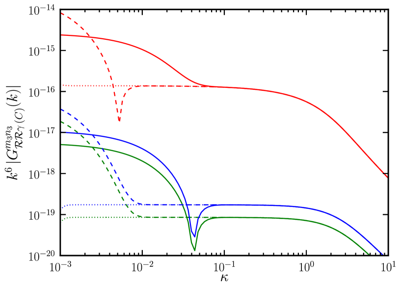
Figure 2: The absolute value of the different contributions to the scalar-scalar-tensor cross-correlation in the equilateral limit, viz. $k^{6}\,G_{{\mathcal{R}}{\mathcal{R}}\gamma}^{m_{3}n_{3}}$, discussed in the previous figure, have been plotted for the same model and mode for a few different combinations of $N_{\rm i}$ and $\kappa$, but with a fixed $N_{\rm s}$ (corresponding to $k/(a\,H)$ of $10^{-5}$). The solid, the dashed and the dotted lines correspond to integrals evaluated from different $N_{\rm i}$, corresponding to $k/(a\,H)$ of $10^{2}$, $10^{3}$ and $10^{4}$, respectively. We should point out that too large a value of $\kappa$ (say, much beyond $\kappa\simeq 0.1$) brings down the values of the integrals, as it then essentially kills the contributions that occur as the modes leave the Hubble radius. It is also evident that the choice of $\kappa=0.1$ and an $N_{\rm i}$ corresponding to $k/(a\,H)=10^{2}$ leads to consistent results (as all the curves converge over this domain). Again, we find that the same conclusions apply to all the contributions to the other three-point functions as well.

We have carried out similar exercises for all the models that we shall discuss in this paper, and we have found that the above set of values for $N_{\rm i}$, $N_{\rm s}$ and $\kappa$ lead to robust results in all the cases. Also, as we shall illustrate in the following sub-section, the numerical results arrived at in such a fashion are consistent with the various analytical results that are available. Actually, we find that, the numerical results obtained with a $\kappa$ of $0.1$ and an $N_{i}$ corresponding to $k/(a\,H)$ of $10^{2}$ matches the analytical results at the level of $5\%$, just as it had in the case of the scalar bi-spectrum [39]. The match improves to $1$–$2\%$ if we work with a $\kappa$ of, say, $0.02$, and simultaneously integrate from an $N_{i}$ corresponding to $k/(a\,H)$ of $10^{3}$. We should emphasize here that we have worked with these set of values in arriving at all the latter figures (i.e. Fig. 3 and thereafter).

3.3 Comparison with the analytical results

In this section, as it was done in the context of the scalar bi-spectrum (see Ref. [39]), we shall compare the numerical results for the three-point functions (or, equivalently, for the non-Gaussianity parameters) with the spectral dependence that can be arrived at in power-law inflation in the equilateral and the squeezed limits and the results for an arbitrary triangular configuration that can be obtained in the slow roll scenario (as applied to the case of the quadratic potential). With the motivation to consider a non-trivial situation involving departures from slow roll, we shall also evaluate the three-point functions for the case of the Starobinsky model analytically and compare them with the corresponding numerical results. We shall relegate some of the details of the calculation in the case of the Starobinsky model to the appendix.

3.3.1 The case of power law inflation

As we have already discussed, power law inflation is described by the scale factor (3.10). Also, in such a scenario, the scalar and the tensor modes $v_{k}$ and ${\mathcal{U}}_{k}$ can be obtained analytically [cf. Eq. (3.11)]. Note that these modes depend only on the combination $k\,\eta$. Due to this reason, interestingly, one finds that, with a simple rescaling of variables, the spectral dependence (but, not the amplitudes) of all the contributions to the scalar-tensor cross correlations as well as the tensor bi-spectrum can be arrived at without actually having to evaluate the integrals involved [39]. Since the solutions to the scalar as well as the tensor modes are of the same form, in the equilateral limit, i.e. when $k_{1}=k_{2}=k_{3}=k$, one finds that all the contributions to the three-point functions have the same spectral dependence, viz. $k^{6}\,G_{{\sf ABC}\,(C)}(k)\propto k^{4\,(\gamma+2)}$.

In fact, in power law inflation, we find that the spectral dependence of all the contributions can also be arrived at in the squeezed limit, which corresponds to setting two of the wavenumbers to be the same, while allowing the third to vanish. Note that, as far as the cross-correlations go, in the squeezed limit, there exist two possibilities. We can either consider the limit wherein the wavenumber of a scalar mode goes to zero or we can consider the situation wherein the wavenumber of a tensor mode vanishes. We obtain the following behavior for $G_{{\mathcal{R}}{\mathcal{R}}\gamma\,(C)}^{m_{3}n_{3}}({\bm{k}}_{1},{\bm{k}}_{2},{\bm{k}}_{3})$ when $k_{1}=k_{2}=k$ and $k_{3}\to 0$ (i.e. when the wavenumber of the tensor mode vanishes):

$$k^{3}\,k_{3}^{3}\,G_{{\mathcal{R}}{\mathcal{R}}\gamma\,(1)}^{m_{3}n_{3}}(k,k_{3}) \propto k^{2\,(\gamma+2)}\,k_{3}^{2\,(\gamma+2)},$$ (3.17a)

$$k^{3}\,k_{3}^{3}\,G_{{\mathcal{R}}{\mathcal{R}}\gamma\,(2)}^{m_{3}n_{3}}(k,k_{3}) \propto k^{2\,(\gamma+1)}\,k_{3}^{2\,(\gamma+3)},$$ (3.17b)

$$k^{3}\,k_{3}^{3}\,G_{{\mathcal{R}}{\mathcal{R}}\gamma\,(3)}^{m_{3}n_{3}}(k,k_{3}) \propto k^{2\,(\gamma+1)}\,k_{3}^{2\,(\gamma+3)},$$ (3.17c)

whereas we find that all the terms have the following spectral dependence as $k_{1}\to 0$ (i.e. as the wavenumber of a scalar mode goes to zero) and $k_{2}=k_{3}=k$:

$$k_{1}^{3}\,k^{3}\,G_{{\mathcal{R}}{\mathcal{R}}\gamma\,(C)}^{m_{3}n_{3}}(k_{1},k)\propto k_{1}^{2\,\gamma+5}\,k^{2\,\gamma+3}.$$ (3.18)

Similarly, in the case of $G_{{\mathcal{R}}\gamma\gamma\,(C)}^{m_{2}n_{2}m_{3}n_{3}}({\bm{k}}_{1},{\bm{k}}_{2},{\bm{k}}_{3})$, when $k_{2}=k_{3}=k$ and $k_{1}\to 0$ (i.e. when the wavenumber of the scalar mode vanishes), we obtain that

$$k_{1}^{3}\,k^{3}\,G_{{\mathcal{R}}\gamma\gamma\,(1)}^{m_{2}n_{2}m_{3}n_{3}}(k_{1},k) \propto k_{1}^{2\,(\gamma+2)}\,k^{2\,(\gamma+2)},$$ (3.19a)

$$k_{1}^{3}\,k^{3}\,G_{{\mathcal{R}}\gamma\gamma\,(2)}^{m_{2}n_{3}m_{3}n_{3}}(k_{1},k) \propto k_{1}^{2\,(\gamma+2)}\,k^{2\,(\gamma+2)},$$ (3.19b)

$$k_{1}^{3}\,k^{3}\,G_{{\mathcal{R}}\gamma\gamma\,(3)}^{m_{2}n_{3}m_{3}n_{3}}(k_{1},k) \propto k_{1}^{2\,(\gamma+3)}\,k^{2\,(\gamma+1)},$$ (3.19c)

whereas we find that all the terms have the following spectral dependence when $k_{1}=k_{2}=k$ and $k_{3}\to 0$ (i.e. as the wavenumber of the tensor mode goes to zero):

$$k^{3}\,k_{3}^{3}\,G_{{\mathcal{R}}\gamma\gamma\,(C)}^{m_{2}n_{2}m_{3}n_{3}}(k,k_{3})\propto k^{2\,(\gamma+1)}\,k_{3}^{2\,(\gamma+3)}.$$ (3.20)

Lastly, one can show that, in power law inflation, in the squeezed limit, say, when $k_{2}=k_{3}=k$ and $k_{1}\to 0$, the two contributions to the tensor bi-spectrum behave as

$$k_{1}^{3}\,k^{3}\,G_{\gamma\gamma\gamma\,(C)}^{m_{1}n_{1}m_{2}n_{2}m_{3}n_{3}}(k_{1},k)\propto k_{1}^{2\,(\gamma+2)}\,k^{2\,(\gamma+2)}.$$ (3.21)

In Figs. 3 and 4, we have compared the spectral dependences we have obtained above in the equilateral and the squeezed limits for all the different contributions to the three-point functions of interest with the corresponding numerical results. We find the agreement between the analytical and the numerical results to be quite good (about $1$-$2\%$, as we have alluded to before).

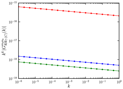
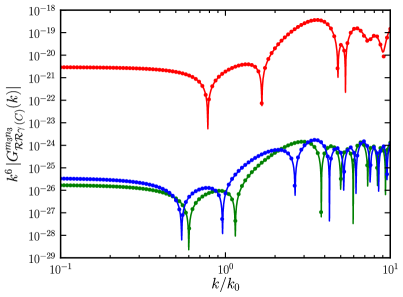
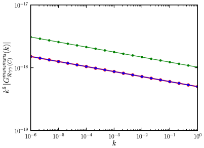
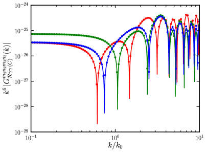
Figure 3: A comparison of the numerical results (plotted as solid lines) with the analytical results (marked with dots) for the various contributions to the three-point functions in the equilateral limit, viz. $k^{6}$ times the absolute values of $G_{{\mathcal{R}}{\mathcal{R}}\gamma\,(C)}^{m_{3}n_{3}}$ (on top), $G_{{\mathcal{R}}\gamma\gamma\,(C)}^{m_{2}n_{2}m_{3}n_{3}}$ (in the middle) and $G_{\gamma\gamma\gamma\,(C)}^{m_{1}n_{1}m_{2}n_{2}m_{3}n_{3}}$ (at the bottom), for power law inflation (on the left) and the Starobinsky model (on the right). In the case of power law inflation, in plotting the analytical, spectral dependences, we have chosen the amplitude by hand so that they match the numerical result at a specific wavenumber. The hierarchy of the different contributions are clear from the above figure. Note that, in the cases of the scalar-tensor-tensor cross-correlation and the tensor bi-spectrum, as is expected from their dependence on the first slow roll parameter $\epsilon_{1}$, the different contributions to these quantities prove to be of the same order. Whereas, in the case of the scalar-scalar-tensor cross-correlation, the second and the third terms are of the same order, but are sub-dominant to the first term.

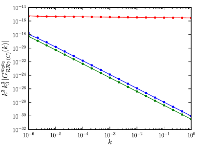
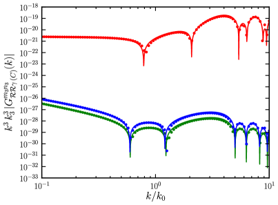
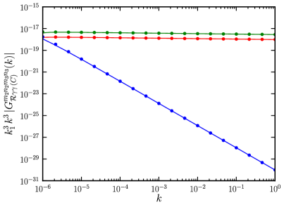
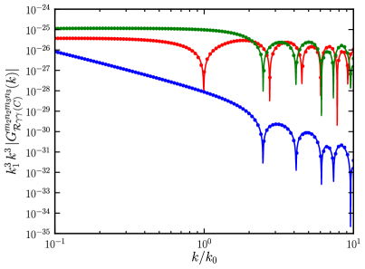
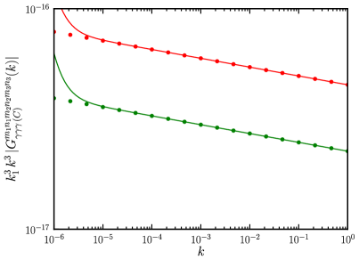
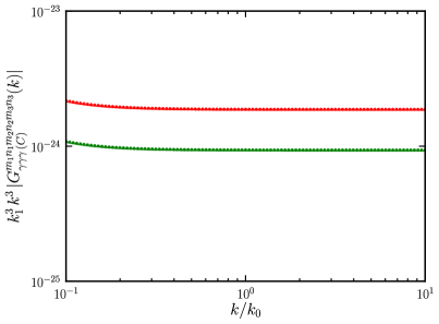
Figure 4: A comparison of the analytic and the numerical results in the squeezed limit for the same set of quantities and models as in the previous figure. Note that, in arriving at the theoretical spectral dependences in the squeezed limit, we have taken the wavenumber of the tensor mode to zero in the case of $G_{{\mathcal{R}}{\mathcal{R}}\gamma}^{m_{3}n_{3}}$ and we have assumed that the wavenumber of the scalar mode vanishes in the case of $G_{{\mathcal{R}}\gamma\gamma}^{m_{2}n_{2}m_{3}n_{3}}$. Clearly, the numerical results match the analytical results quite well in the equilateral limit. However, in the squeezed limit, while the match is good at large $k$, there is a noticeable difference between the theoretical and the numerical results at small $k$ in some cases. This difference essentially arises due to the fact that, while the theoretical results have been arrived at by assuming that one of the wavenumbers (either $k_{1}$ or $k_{3}$) vanishes, it is impossible to set a wavenumber to be zero numerically and one has to work with a suitably small value that permits the evolution of the modes as well as the evaluation of the integrals involved. We have chosen the value of the large scale mode $k_{1}$ or $k_{3}$ to be $8.3\times 10^{-7}$ and $4.3\times 10^{-2}\,k_{0}$ in the power law case and the Starobinsky model, respectively. If needed, the match can be improved by working with a smaller wavenumber, but the effort can become numerically taxing.

3.3.2 Comparison in the case of the Starobinsky model

The Starobinsky model is characterized by a linear potential with a sharp change in slope at a specific point [33]. The potential that governs the model is given by

$$V(\phi)=\left\{\begin{array}[]{rcl}V_{0}+A_{+}(\phi-\phi_{0})&{\rm for}&\phi>\phi_{0},\\ V_{0}+A_{-}(\phi-\phi_{0})&{\rm for}&\phi<\phi_{0},\end{array}\right.$$ (3.22)

where $V_{0}$, $A_{+}$, $A_{-}$ and $\phi_{0}$ are constants. Evidently, the derivative of the potential contains a discontinuity at $\phi_{0}$. The discontinuity leads to a brief period of fast roll as the field crosses the point, before slow roll is restored again at late times. It is assumed that the constant term $V_{0}$ in the potential is dominant as the transition across the discontinuity takes place. Hence, the scale factor always behaves as that of de Sitter with the constant Hubble parameter, say, $H_{0}$, being given by $H_{0}^{2}\simeq V_{0}/(3\,M_{{}_{\rm Pl}}^{2})$ (for recent discussions on the evolution of the background as well as the perturbations, see Refs. [43, 44]).

Note that the only background quantity required to evaluate the tensor bi-spectrum is the scale factor $a$ [cf. Eqs. (2.23)]. Since, in the Starobinsky model, the scale factor is always of the de Sitter form, i.e. $a(\eta)=-1/(H_{0}\,\eta)$, the tensor modes remain unaffected by the transition. As a result, the tensor bi-spectrum that one arrives at in this case is essentially the same as the one obtained in the slow roll approximation (to be precise, in the de Sitter limit). As far as the three-point cross-correlations are concerned, we require, apart from the scale factor, the behavior of the first slow roll parameter $\epsilon_{1}$ as well [cf. Eqs. (2.17) and (2.19)]. Let us denote the various quantities before and after the transition by the sub-scripts (or super-scripts, as is convenient) plus and minus, respectively. One finds that the behavior of the first slow roll parameter $\epsilon_{1}$ can be expressed as [43, 44]

$$\epsilon_{1+} \simeq \frac{A_{+}^{2}}{18\,M_{{}_{\rm Pl}}^{2}\,H_{0}^{4}},$$ (3.23a)

$$\epsilon_{1-} \simeq \frac{A_{-}^{2}}{18\,M_{{}_{\rm Pl}}^{2}\,H_{0}^{4}}\,\left[1+\rho^{3}\,\eta^{3}\right]^{2},$$ (3.23b)

where $\rho^{3}=-(\Delta A/A_{-})\,\,(1/\eta_{0})^{3}$, with $\Delta A=A_{-}-A_{+}$ and $\eta_{0}$ being the conformal time at the transition. Actually, as we shall see below, the derivative of the scalar modes which are required to evaluate the three-point functions also involve the second slow roll parameter $\epsilon_{2}={\rm d}\,{\rm ln}\,\epsilon_{1}/{\rm d}N$. It can be shown that the second slow roll parameter behaves as follows [43, 44]:

$$\epsilon_{2+} \simeq 4\,\epsilon_{1+},$$ (3.24a)

$$\epsilon_{2-} \simeq \frac{-\,6\,\rho^{3}\,\eta^{3}}{1+\rho^{3}\,\eta^{3}}.$$ (3.24b)

Evidently, we also require the scalar and the tensor modes, $f_{k}$ and $g_{k}$, as well as their derivatives with respect to the conformal time, in order to arrive at the three-point functions. As we have already mentioned, since the scale factor remains unaffected by the transition, the tensor modes are given by the standard Bunch-Davies solutions in the de Sitter spacetime, viz.

$$g_{k}(\eta)=\frac{i\,\sqrt{2}\;H_{0}}{M_{{}_{\rm Pl}}\,\sqrt{2\,k^{3}}}\,\left(1+i\,k\,\eta\right)\,{\rm e}^{-i\,k\,\eta},$$ (3.25)

the time derivative of which is straightforward to evaluate. The scalar modes $f_{k}$ before and after the transition can be expressed as [43, 44]:

$$f_{k}^{+}(\eta) = \frac{i\,H_{0}}{2\,M_{{}_{\rm Pl}}\,\sqrt{{k^{3}}\,\epsilon_{1+}}}\,\left(1+i\,k\,\eta\right)\,{\rm e}^{-i\,k\,\eta},$$ (3.26a)

$$f_{k}^{-}(\eta) = \frac{i\,H_{0}\,\alpha_{k}}{2\,M_{{}_{\rm Pl}}\,\sqrt{{k^{3}}\,\epsilon_{1-}}}\,\left(1+i\,k\,\eta\right)\,{\rm e}^{-i\,k\,\eta}-\frac{i\,H_{0}\,\beta_{k}}{2\,M_{{}_{\rm Pl}}\,\sqrt{{k^{3}}\,\epsilon_{1-}}}\left(1-i\,k\,\eta\right)\,{\rm e}^{i\,k\,\eta}.$$ (3.26b)

The derivatives of $f_{k}$ can be obtained to be, at the level of the approximation one works in,

$$f_{k}^{+}{}^{\prime}(\eta) = \frac{i\,H_{0}}{2\,M_{{}_{\rm Pl}}\,\sqrt{{k^{3}}\,\epsilon_{1+}}}\;k^{2}\,\eta\;{\rm e}^{-i\,k\,\eta},$$ (3.27)

$$f_{\bm{k}}^{-}{}^{\prime}(\eta) = \frac{i\,H_{0}\,\alpha_{k}}{2\,M_{{}_{\rm Pl}}\,\sqrt{{k^{3}}\epsilon_{1-}}}\left[\frac{\epsilon_{2-}}{2\,\eta}\,\left(1+i\,k\,\eta\right)+k^{2}\,\eta\right]\,{\rm e}^{-i\,k\,\eta}$$ (3.28)

$$- \frac{i\,H_{0}\,\beta_{k}}{2\,M_{{}_{\rm Pl}}\,\sqrt{{k^{3}}\epsilon_{1-}}}\left[\frac{\epsilon_{2-}}{2\,\eta}\,\left(1-i\,k\,\eta\right)+k^{2}\,\eta\right]{\rm e}^{i\,k\,\eta}.$$

The quantities $\alpha_{k}$ and $\beta_{k}$ that appear in the above expressions are the standard Bogoliubov coefficients, which are obtained by matching the modes $f_{k}$ and their derivatives $f_{k}^{\prime}$ at the transition. They are found to be [33, 43, 44]

$$\alpha_{\bm{k}} = 1+\frac{3\,i\,\Delta A}{2\,A_{+}}\;\frac{k_{0}}{k}\,\left(1+\frac{k_{0}^{2}}{k^{2}}\right),$$ (3.29a)

$$\beta_{\bm{k}} = -\frac{3\,i\,\Delta A}{2\,A_{+}}\;\frac{k_{0}}{k}\,\left(1+\frac{i\,k_{0}}{k}\right)^{2}\,{\rm e}^{2\,i\,k/k_{0}},$$ (3.29b)

with $k_{0}=-1/\eta_{0}=a_{0}\,H_{0}$ and $a_{0}$ being the value of the scale factor at the transition.

We have already mentioned that, in the Starobinsky model, the tensor bi-spectrum will essentially be the same as the one arrived at in the slow roll approximation (in this context, see, for instance, Refs. [11, 16]). Note that since the scalar modes (and the first two slow roll parameters) behave differently before and after the transition, while evaluating the scalar-tensor cross-correlations, one needs to divide the integrals involved into two, and carry out the integrals before and after the transition separately, just as it was done in the context of the scalar bi-spectrum [43, 44]. We find that the cross-correlations can be evaluated completely analytically for an arbitrary triangular configuration of the wavenumbers (which, in fact, proves to be difficult to carry out for the scalar bi-spectrum). Since the calculations and the expressions involved prove to be rather long and cumbersome, we have relegated the calculations to the appendix. In Figs. 3 and 4, we have compared the analytic results we have obtained with the corresponding numerical results for the cross-correlations and the tensor bi-spectrum in the equilateral and the squeezed limits. We should mention here that, in order to solve the problem numerically, the discontinuity in the potential of the Starobinsky model has been suitably smoothened [39]. The figures suggest that the match between the analytic and the numerical results is very good.

3.3.3 The case of the quadratic potential

As is well known, the conventional quadratic potential leads to slow roll and, hence, in this case, one can utilize the three-point functions evaluated in the slow roll limit to compare with the numerical results. For the sake of completeness, we shall write down here the entire expressions for the non-Gaussianity parameters evaluated in the slow roll approximation. We find that, if we ignore factors involving $\Pi_{mn,ij}^{{\bm{k}}}$, they are given by

$$C_{{}_{\rm NL}}^{\mathcal{R}} = \left(k_{2|\ast}^{n_{{}_{\rm S}}-1}\,k_{3|\ast}^{n_{{}_{\rm T}}}+k_{2|1}^{3}\,k_{1|\ast}^{n_{{}_{\rm S}}-1}\,k_{3|*}^{n_{{}_{\rm T}}}\right)^{-1}$$ (3.30b)

$$\times\,\left[k_{2|1}\,k_{{{}_{\rm T}}|1}\,\left(1-\frac{k_{2|1}+k_{3|1}+k_{2|1}\,k_{3|1}}{k_{{{}_{\rm T}}|1}^{2}}-\frac{k_{2|1}\,k_{3|1}}{k_{{{}_{\rm T}}|1}^{3}}\right)-\epsilon_{1}\,\frac{k_{2|1}\,k_{3|1}^{2}}{k_{{{}_{\rm T}}|1}}\right],$$

$$= \left(k_{1|3}^{3}\,k_{2|\ast}^{n_{{}_{\rm S}}-1}\,k_{3|\ast}^{n_{{}_{\rm T}}}+k_{2|3}^{3}\,k_{1|\ast}^{n_{{}_{\rm S}}-1}\,k_{3|*}^{n_{{}_{\rm T}}}\right)^{-1},$$

$$\times\,\left[k_{1|3}\,k_{2|3}\,k_{{{}_{\rm T}}|3}\,\left(1-\frac{k_{1|3}+k_{2|3}+k_{1|3}\,k_{2|3}}{k_{{{}_{\rm T}}|3}^{2}}-\frac{k_{1|3}\,k_{2|3}}{k_{{{}_{\rm T}}|3}^{3}}\right)-\epsilon_{1}\,\frac{k_{1|3}\,k_{2|3}}{k_{{{}_{\rm T}}|3}}\right],\quad$$

$$C_{{}_{\rm NL}}^{\mathcal{\gamma}} = \frac{\epsilon_{1}}{4}\,\left(k_{3|1}^{3}\,k_{1|\ast}^{n_{{}_{\rm S}}-1}\,k_{2|\ast}^{n_{{}_{\rm T}}}+k_{2|1}^{3}\,k_{1|\ast}^{n_{{}_{\rm S}}-1}\,k_{3|*}^{n_{{}_{\rm T}}}\right)^{-1}\,\left(1-k_{2|1}^{2}-k_{3|1}^{2}-\frac{8\,k_{2|1}^{2}\,k_{3|1}^{2}}{k_{{{}_{\rm T}}|1}}\right),$$ (3.30c)

$$= \frac{\epsilon_{1}}{4}\,\left(k_{1|\ast}^{n_{{}_{\rm S}}-1}\,k_{2|\ast}^{n_{{}_{\rm T}}}+k_{2|3}^{3}\,k_{1|\ast}^{n_{{}_{\rm S}}-1}\,k_{3|*}^{n_{{}_{\rm T}}}\right)^{-1}\,\left(k_{1|3}^{3}-k_{1|3}\,\left(1+k_{2|3}^{2}\right)-\frac{8\,k_{2|3}^{2}}{k_{{{}_{\rm T}}|3}}\right),$$ (3.30d)

$$h_{{}_{\rm NL}} = \left(k_{2|*}^{n_{{}_{\rm T}}}\,k_{3|*}^{n_{{}_{\rm T}}}\,+k_{2|1}^{3}\,k_{1|*}^{n_{{}_{\rm T}}}\,k_{3|*}^{n_{{}_{\rm T}}}+k_{3|1}^{3}\,k_{1|*}^{n_{{}_{\rm T}}}\,k_{2|*}^{n_{{}_{\rm T}}}\right)^{-1}\,\left(1+k_{2|1}+k_{3|1}\right)\,\left(1+k_{2|1}^{2}+k_{3|1}^{2}\right)$$ (3.30e)

$$\times\,\left(1-\frac{k_{2|1}+k_{3|1}+k_{2|1}\,k_{3|1}}{k_{{{}_{{\rm T}}|1}^{2}}}-\frac{k_{2|1}\,k_{3|1}}{k_{{{}_{\rm T}}|1}^{3}}\right),$$

where $k_{i|j}=k_{i}/k_{j}$, $k_{i|\ast}=k_{i}/k_{\ast}$, $k_{{{}_{\rm T}}|1}=1+k_{2|1}+k_{3|1}$ and $k_{{}_{{\rm T}}|3}=k_{1|3}+k_{2|3}+1$. Recall that, in the slow roll approximation, $n_{{}_{\rm S}}=1-2\,\epsilon_{1}-\epsilon_{2}$, while $n_{{}_{\rm T}}=-2\,\epsilon_{1}$. In Fig. 5, we have plotted the above analytical results for the non-Gaussianity parameters and the corresponding numerical results for an arbitrary triangular configuration of the wavenumbers for the case of the quadratic potential.

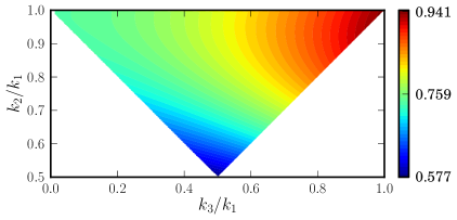
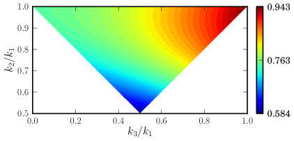
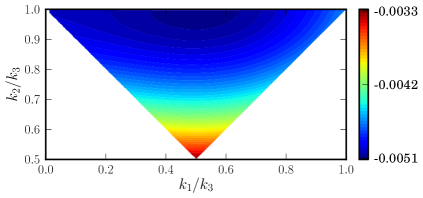
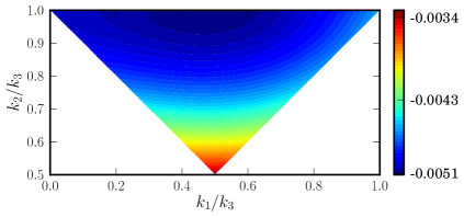
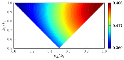
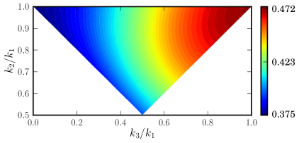
Figure 5: Density plots of the non-Gaussianity parameters $C_{{}_{\rm NL}}^{\mathcal{R}}$ (on top), $C_{{}_{\rm NL}}^{\mathcal{\gamma}}$ (in the middle) and $h_{{}_{\rm NL}}$ (at the bottom) for an arbitrary triangular configuration of the wavenumbers for the case of the conventional, quadratic potential. In arriving at the above figures, when $k_{1}$ and $k_{3}$ appear in the denominators of the two axes, we have chosen them to be $k_{\ast}$. Evidently, the strong similarity between the numerical results (on the left) and the corresponding quantities arrived at using the slow roll approximation (on the right) indicates the robustness of the numerical procedure we have adopted to compute the three-point functions. We find that the numerical results match the analytical estimates to better than $1\%$ over a large domain of the wavenumbers of interest.

There is clearly a striking similarity between the structure of the numerical results and the corresponding analytical estimates. We find that the numerical and analytical results match to better than $1\%$ over a large region of the wavenumbers involved.

4 The three-point functions in models leading to features in the scalar power spectrum

As we had discussed in the introduction, there has been considerable interest in studying the possibility of features in the scalar power spectrum over the last decade. Specifically, a large amount of attention has been focused on models leading to three types of features, viz. a sharp cut-off on large scales, a burst of oscillations over an intermediate range of scales and small but repeated oscillations over a wide range of scales (in this context, see Refs. [20, 21, 22, 23, 24, 25, 26, 27, 28, 29]). And, not surprisingly, it is exactly such classes of models that have been considered by the Planck team [8].

In this section, we shall utilize our code to study the behavior of the three-point functions of interest in models leading to deviations from slow roll. We shall consider three different models that lead to features in the scalar power spectrum of the three types mentioned above (see, in this context, Fig. 9 of Ref. [39]). The first of the models that we shall consider is the model described by the following potential:

$$V(\phi)=\frac{m^{2}}{2}\,\phi^{2}-\frac{\sqrt{2\,\lambda\,(n-1)}\,m}{n}\,\phi^{n}+\frac{\lambda}{4}\,\phi^{2\,(n-1)}.$$ (4.1)

For suitable values of the parameters, this model leads to a brief period of departure from inflation before slow roll is restored again, a scenario that has been dubbed punctuated inflation [20]. Due to the sudden deviation from slow roll that one encounters, this model leads to sharp features in the scalar power as well as bi-spectra [20, 39].

The second model that we shall consider is the one described by the popular quadratic potential, but with an additional step that has been introduced by hand. The complete potential is given by the expression [21, 22, 23]

$$V(\phi)=\frac{m^{2}}{2}\,\phi^{2}\,\left[1+\alpha\,\tanh\,\left(\frac{\phi-\phi_{0}}{\Delta\phi}\right)\right],$$ (4.2)

where, clearly, $\alpha$ and $\Delta\phi$ denote the height and the width of the step, respectively, while $\phi_{0}$ represents its location.

The last model that we shall consider is the so-called axion monodromy model that consists of a linear potential with super-imposed oscillations. The potential is motivated by string theory and is given by [26, 28, 29]

$$V(\phi)=\lambda\,\left[\phi+\alpha\,\cos\,\left(\frac{\phi}{\beta}+\delta\right)\right].$$ (4.3)

We have evaluated the scalar-tensor cross-correlations and the tensor bi-spectrum numerically for the three models listed above. We should mention here that we have worked with parameters for the models that lead to an improved fit to the WMAP seven [4] or nine-year data [5]. (We would refer the reader to the earlier effort [39] to calculate the scalar bi-spectrum in these models for the values of the potential parameters, including that of the Starobinsky model which we had discussed before. We would also refer the reader to Fig. 8 of the work for a plot of the various potentials.) It is important that we add here that models such as the quadratic potential with the step and the axion monodromy model have very recently been compared with the Planck data (see Refs. [50] and [51, 52, 53]). These investigations suggest that the resulting features lead to an improved fit to the Planck data too. Moreover, models similar to punctuated inflation, which lead to suppression of power on large scales continue to attract attention as well (in this context, see Refs. [54]). In Fig. 6, we have plotted the three non-Gaussianity parameters, viz. $C_{{}_{\rm NL}}^{\mathcal{R}}$, $C_{{}_{\rm NL}}^{\mathcal{\gamma}}$ and $h_{{}_{\rm NL}}$, for the above three models for an arbitrary triangular configuration of the wavenumbers.

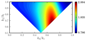
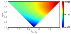
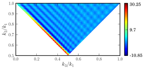
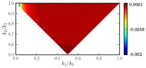
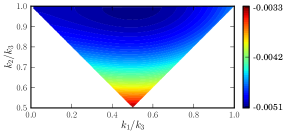
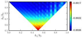
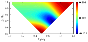
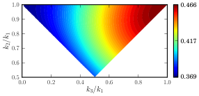
Figure 6: Density plots of the non-Gaussianity parameters $C_{{}_{\rm NL}}^{\mathcal{R}}$ (on top), $C_{{}_{\rm NL}}^{\mathcal{\gamma}}$ (in the middle) and $h_{{}_{\rm NL}}$ (at the bottom) evaluated numerically for an arbitrary triangular configuration of the wavenumbers for the case of the punctuated inflationary scenario (the left column), the quadratic potential with the step (the middle column) and the axion monodromy model (the right column). It should be evident that, in models leading to features, the shape of the three-point functions as plotted against $k_{3}/k_{1}$ and $k_{2}/k_{1}$ in the cases of $C_{{}_{\rm NL}}^{\mathcal{R}}$ and $h_{{}_{\rm NL}}$ or, against $k_{1}/k_{3}$ and $k_{2}/k_{3}$ in the case of $C_{{}_{\rm NL}}^{\mathcal{\gamma}}$, will depend on the choices of denominators $k_{1}$ and $k_{3}$. In order to capture the non-trivial shapes that these models lead to, we have fixed $k_{1}$ and $k_{3}$ (when they appear in the denominators) to be $10^{-3}$, $2\times 10^{-3}$ and $5\times 10^{-2}$ in the cases of punctuated inflation, the quadratic potential with a step and the monodromy model, respectively.

Let us now highlight certain aspects of the results that we have obtained. We had earlier pointed out (see the caption of Fig. 3) the hierarchy of the various contributions to the three-point functions. We find that the hierarchy is maintained even when deviations from slow roll occurs. This is not surprising because the tensor bi-spectrum is independent of the slow roll parameters, whereas the cross-correlations at the most depend on the first slow roll parameter $\epsilon_{1}$. Since the first slow roll parameter cannot remain large for an extended period without completely terminating inflation, the hierarchy of the different contributions is preserved even in situations involving departures from slow roll.

It is clear from Fig. 6 that the tensor bi-spectrum in the cases of the quadratic potential with the step and the axion monodromy model resemble each other very closely. In fact, they have virtually the same amplitude and shape as in the slow roll case illustrated in Fig. 5. This should not be surprising. After all, since the deviations from slow roll are rather minimal in these models, the tensors are hardly affected. In contrast, punctuated inflation, because of the brief departure from accelerated expansion that occurs, leads to a rather large effect on the tensors, with the tensor amplitude being considerably suppressed on small scales [20]. This is reflected in the non-trivial shape of the associated $h_{{}_{\rm NL}}$ parameter. The ringing effects on the scalars that arises due to the resonance encountered in the monodromy model (see, for example, Refs. [26, 28]) is clearly reflected in the amplitudes and shapes of the corresponding $C_{{}_{\rm NL}}^{\mathcal{R}}$ and the $C_{{}_{\rm NL}}^{\mathcal{\gamma}}$ parameters. It is this resonance that leads to a substantially larger value for the $C_{{}_{\rm NL}}^{\mathcal{R}}$ parameter, as it does to the scalar non-Gaussianity parameter $f_{{}_{\rm NL}}$ (in this context, see, for instance, Ref. [39]). Note that, apart from the ringing, the shape of the $C_{{}_{\rm NL}}^{\mathcal{\gamma}}$ parameter is somewhat similar in the cases of the quadratic potential with the step and the monodromy model. In the case of punctuated inflation, the shape of the $C_{{}_{\rm NL}}^{\mathcal{R}}$ and $C_{{}_{\rm NL}}^{\mathcal{\gamma}}$ parameters are considerably influenced by the contrasting fall and rise of the scalar and the tensor powers at large scales. This behavior results in a larger value for the $C_{{}_{\rm NL}}^{\mathcal{R}}$ parameter than the corresponding value encountered in, say, the case of the model with the step.

5 The contributions during preheating

In most models of inflation, the scalar field rolls down the potential and inflation is terminated when the field is close to a mimina of the potential. Thereafter, typically, the scalar field oscillates at the bottom of the potential. During this epoch, the inflaton, due to its coupling to the matter fields, is expected to decay and thermalize, thereby leading to the conventional radiation dominated era [40].

Immediately after inflation and before the inflaton starts decaying, there exists a brief domain when the scalar field is oscillating at the bottom of the potential and continues to dominate the background evolution. This brief epoch is referred to as preheating [40]. Since the scalar field is the dominant source of the background, the perturbations (both scalar and tensor) continue to be governed by the same actions and equations of motion as they are during inflation. It is interesting to then investigate the contributions to the three-point functions that we have considered due to this epoch. In fact, the contributions to the scalar bi-spectrum during preheating in single field inflationary models was evaluated recently [42]. Our aim in this section is to extend the analysis to the case of the other three-point functions.

In order to do so, as should be clear by now, we require the behavior of the background as well as the perturbations during the epoch of preheating. If one considers single field inflationary models with quadratic minima, say, $V(\phi)\simeq m^{2}\,\phi^{2}/2$, then it can be shown that, during the epoch of preheating, the first slow roll parameter behaves as [40, 41, 42]

$$\epsilon_{1}\simeq 3\,\cos^{2}(m\,t+\Delta),$$ (5.1)

where $t$ is the cosmic time (measured since the end of inflation), while $\Delta$ is an arbitrary phase, chosen suitably to match the transition from inflation to preheating. The average value of the above slow roll parameter is $3/2$, which corresponds to a matter dominated era. Note that, all perturbations of cosmological interest are on super-Hubble scales during the domain of preheating. Naively, one may imagine that the super-Hubble solutions for the scalar and the tensor perturbations during inflation, as given by Eqs. (3.2), will continue to hold during the epoch of preheating too. The tensor modes are governed by the quantity $a^{\prime\prime}/a$, which behaves monotonously during inflation as well as preheating. Therefore, the $k^{2}$ term in Eq. (3.1b) can indeed be ignored when compared to $a^{\prime\prime}/a$ even during preheating, so that the super-Hubble solutions to the tensor modes, viz. Eq. (3.2b), continue to be applicable [41]. However, the quantity $z^{\prime\prime}/z$, as it involves the scalar field, behaves differently during inflation and preheating. While it grows monotonically during the latter stages of inflation, the quantity can even vanish during preheating (since the scalar field is oscillating at the minimum of the potential). Hence, it is not a priori clear that the inflationary, super-Hubble, solutions will remain valid once the accelerated expansion has terminated. A careful analysis however illustrates that, under certain conditions which are easily achieved in quadratic minima (for details, see, for instance, Refs. [41, 42]), the inflationary super-Hubble solutions for the scalar modes continue to be applicable during preheating.

Recall that the contributions to the tensor bi-spectrum (and, hence, to the corresponding non-Gaussianity parameter $h_{{}_{\rm NL}}$) on super-Hubble scales during inflation is strictly zero. This is true even during the epoch of preheating. For simplicity, let us ignore the oscillations at the bottom of the quadratic minima and use the average value of the first slow roll parameter, viz. that $\epsilon_{1}\simeq 3/2$. In such a case, if one focuses on the equilateral limit, one can show that the contribution to the non-Gaussianity parameters $C_{{}_{\rm NL}}^{\mathcal{R}}$ and $C_{{}_{\rm NL}}^{\mathcal{\gamma}}$ arising due to the evolution from the end of inflation to the e-fold, say, $N_{\rm f}$, during preheating can be expressed as

$$C_{{}_{\rm NL}}^{{\mathcal{R}}\,({\rm ef})}(k)=\left(\frac{4\,\gamma+5}{5\,\gamma+7}\right)\;C_{{}_{\rm NL}}^{\gamma\,({\rm ef})}(k)=\frac{12}{115}\,\left(\frac{4\,\gamma+5}{\gamma+2}\right)\;f_{{}_{\rm NL}}^{\,({\rm ef})}(k),$$ (5.2)

where $f_{{}_{\rm NL}}^{\,({\rm ef})}$ is the contribution due to preheating to the non-Gaussianity parameter associated with the scalar bi-spectrum and is given by [39]

$$f_{{}_{\rm NL}}^{\,({\rm ef})}(k) = \frac{115\,(\gamma+2)}{288\,\pi\,(\gamma+1)}\;\Gamma^{2}\left(\gamma+\frac{1}{2}\right)\,2^{2\,\gamma+1}\,\left(2\,\gamma+1\right)^{2}\,\sin\,(2\,\pi\,\gamma)$$ (5.3)

$$\times\,\left|\gamma+1\right|^{-2\,(\gamma+1)}\,\left[1-{\rm e}^{-3\,(N_{\rm f}-N_{\rm e})/2}\right]$$

$$\times\,\left[\left(\frac{\pi^{2}\,g_{\rm eff}}{30}\right)^{-1/4}\,\left(1+z_{\rm eq}\right)^{1/4}\,\frac{\rho_{\rm cri}^{1/4}}{T_{\rm rh}}\right]^{-(2\,\gamma+1)}\,\left(\frac{k}{a_{\rm now}\,H_{\rm now}}\right)^{-(2\,\gamma+1)}.$$

We should mention here that we have arrived at this expression assuming inflation to be of the power law form, with the scale factor being given by Eq. (3.10) and with $\epsilon_{1}=(\gamma+2)/(\gamma+1)$, as we have pointed out earlier. In the above expression, the quantity $g_{\rm eff}$ denotes the effective number of relativistic degrees of freedom at reheating, $T_{\rm rh}$ the reheating temperature and $z_{\rm eq}$ the redshift at the epoch of equality. Also, $\rho_{\rm cri}$, $a_{\rm now}$ and $H_{\rm now}$ represent the critical energy density, the scale factor and the Hubble parameter today, respectively. It should be clear from the above expression that the contributions due to preheating is mainly determined by the quantity $\rho_{\rm cri}^{1/4}/T_{\rm rh}$. For an inflationary model wherein $\gamma\simeq-2$ and a reheating temperature of $T_{\rm rh}\simeq 10^{10}\,\mbox{GeV}$, one obtains that $f_{{}_{\rm NL}}^{\,({\rm ef})}\sim C_{{}_{\rm NL}}^{{\mathcal{R}}\,({\rm ef})}\sim C_{{}_{\rm NL}}^{\gamma\,({\rm ef})}\sim 10^{-60}$ for the modes of cosmological interest (i.e. for wavenumbers such that $k\simeq a_{\rm now}\,H_{\rm now}$). Needless to add, these values are simply unobservable (also see, Ref. [55]; in this context, however, see Ref. [56]). In other words, as in the case of the scalar parameter $f_{{}_{\rm NL}}$, the contribution to the other non-Gaussianity parameters due to the epoch of preheating is completely insignificant.

6 Discussion

In this work, based on the Maldacena formalism and extending the recent effort towards calculating the scalar bi-spectrum, we have developed a numerical procedure for calculating the other three-point functions of interest. Motivated by the parameters often introduced to characterize the scalar and the tensor bi-spectra, we have introduced dimensionless non-Gaussianity parameters to describe the scalar-tensor cross-correlations. We have compared the performance of the code with the analytical results that are available in different situations and have utilized the code to calculate the three-point functions and the corresponding non-Gaussianity parameters in a class of models that lead to features in the scalar power spectrum. We have also shown that, as in the case of the scalar bi-spectrum, the contributions to the other three-point functions during the epoch of preheating proves to be completely negligible. In fact, we have made available a sample of the numerical code that we have worked with to arrive at the results discussed in this paper at the following URL: https://www.physics.iitm.ac.in/~sriram/tpf-code/registration.html. The sample code corresponds to the specific case of the quadratic potential with the step that we have considered. The code can be easily extended to other inflationary models.

Before we conclude, we would like to make a couple of clarifying remarks concerning the status of models leading to features in the scalar power spectrum in the light of the Planck data. While, as we had mentioned in the introduction, the Bayesian evidence for features do not seem substantial [8], model independent reconstruction efforts seem to consistently point to the possibility of scale-dependent power spectra (in this context, see the recent efforts, Refs. [57]). Importantly, the Planck team finds that the constraints on the scalar non-Gaussianity parameters $f_{{}_{\rm NL}}$ (that we had quoted in the introductory section) turn less stringent when one permits features (contrast, for instance, Table 8 with Tables 12 and 13 of Ref. [9]). This is an aspect that seems to deserve closer examination.

We believe that the non-Gaussianity parameters $C_{{}_{\rm NL}}^{\mathcal{R}}$ and $C_{{}_{\rm NL}}^{\mathcal{\gamma}}$ which we have introduced here provide additional quantities to characterize an inflationary model. It will be interesting to arrive at constraints on these parameters as well from the observational data and understand its implications. We are currently investigating these issues.

Appendix A Three-point functions in the Starobinsky model

In this appendix, we shall provide some of the essential details for arriving at the analytical results for the three-point functions of our interest in the case of the Starobinsky model [33, 43, 44]. In Subsec. 3.3.2, we have already discussed the behavior of the background as well as the perturbations in the model. It is just a matter of substituting the various quantities in the integrals that describe the three-point functions and being able to carry out the integrals involved. As we had pointed out earlier, due to the transition at the discontinuity in the potential, the integrals need to be divided into two. The integrals up to the transition essentially lead to the slow roll results, but with suitable modifications that arise because of the reason that the integrals are not to be carried out until late times. Though slow roll is violated briefly due to the discontinuity, we find that all the integrals can be evaluated in terms of simple functions to arrive at the three-point correlations. Since the scale factor is always of the de Sitter form, as we had mentioned, the tensor bi-spectrum proves to be the same as the one arrived at in the slow roll approximation [11, 16]. Therefore, we do not discuss it here. In what follows, we shall list out the results of the integrals involved in arriving at the two cross-correlations.

A.1 Calculation of ${\mathcal{G}}_{{\mathcal{R}}{\mathcal{R}}\gamma}^{C}$

Evidently, the quantities ${\cal G}_{{\mathcal{R}}{\mathcal{R}}\gamma}^{C}$, with $C=(1,2,3)$ [cf. Eqs. (2.17a)–(2.17c)], need to be first evaluated in order to arrive at the cross-correlation $G_{{\mathcal{R}}{\mathcal{R}}\gamma}^{m_{3}n_{3}}$. Upon dividing the integrals into two, we find that the contributions before the transition are given by the following expressions:

$${\cal G}_{{\cal R}{\cal R}\gamma}^{1+}({\bm{k}}_{1},{\bm{k}}_{2},{\bm{k}}_{3}) = \frac{H_{0}}{2\,M_{{}_{\rm Pl}}^{3}\,\sqrt{k_{1}^{3}\,k_{2}^{3}\,k_{3}^{3}}}\;\varepsilon_{ij}^{s_{3}\ast}(k_{3})\;k_{1i}\,k_{2j}\;\biggl{[}k_{0}+\frac{i\,\left(k_{1}\,k_{2}+k_{1}\,k_{3}+k_{2}\,k_{3}\right)}{k_{{}_{\rm T}}}$$ (A.1a)

$$-\,\frac{k_{1}\,k_{2}\,k_{3}}{k_{{}_{\rm T}}\,k_{0}}+\frac{i\,k_{1}\,k_{2}\,k_{3}}{k_{{}_{\rm T}}^{2}}\biggr{]}\,{\rm e}^{-i\,k_{{}_{\rm T}}/k_{0}},$$

$${\cal G}_{{\cal R}{\cal R}\gamma}^{2+}({\bm{k}}_{1},{\bm{k}}_{2},{\bm{k}}_{3}) = \frac{A_{+}^{2}}{144\,H_{0}^{3}\,M_{{}_{\rm Pl}}^{5}\,\sqrt{k_{1}^{3}\,k_{2}^{3}\,k_{3}^{3}}}\;\varepsilon_{ij}^{s_{3}\ast}(k_{3})\;k_{1i}\,k_{2j}\,k_{3}^{2}$$ (A.1b)

$$\times\,\left[\frac{i}{k_{{}_{\rm T}}}-\frac{k_{3}}{k_{{}_{\rm T}}\,k_{0}}+\frac{i\,k_{3}}{k_{{}_{\rm T}}^{2}}\right]\,{\rm e}^{-i\,k_{{}_{\rm T}}/k_{0}},$$

$${\cal G}_{{\cal R}{\cal R}\gamma}^{3+}({\bm{k}}_{1},{\bm{k}}_{2},{\bm{k}}_{3}) = -\,\frac{A_{+}^{2}}{144\,H_{0}^{3}\,M_{{}_{\rm Pl}}^{5}\,\sqrt{k_{1}^{3}\,k_{2}^{3}\,k_{3}^{3}}}\;\varepsilon_{ij}^{s_{3}\ast}(k_{3})\;k_{1i}\,k_{2j}\,k_{3}^{2}\;\bigg{[}\left(-\frac{i}{k_{{}_{\rm T}}}+\frac{k_{1}}{k_{{}_{\rm T}}\,k_{0}}-\frac{i\,k_{1}}{k_{{}_{\rm T}}^{2}}\right)$$ (A.1c)

$$+\,\left(-\frac{i}{k_{{}_{\rm T}}}+\frac{k_{2}}{k_{{}_{\rm T}}\,k_{0}}-\frac{i\,k_{2}}{k_{{}_{\rm T}}^{2}}\right)\biggr{]}\,{\rm e}^{-i\,k_{{}_{\rm T}}/k_{0}},$$

where, as we have indicated earlier, $k_{{}_{\rm T}}=k_{1}+k_{2}+k_{3}$. Similarly, after the transition, upon substituting the corresponding modes describing the perturbations, we find that, we can write

$${\cal G}_{{\cal R}{\cal R}\gamma}^{1-}({\bm{k}}_{1},{\bm{k}}_{2},{\bm{k}}_{3}) = \frac{H_{0}}{2\,M_{{}_{\rm Pl}}^{3}\,\sqrt{k_{1}^{3}\,k_{2}^{3}\,k_{3}^{3}}}\;\varepsilon_{ij}^{s_{3}\ast}(k_{3})\;k_{1i}\,k_{2j}\,\biggl{[}\alpha_{k_{1}}^{\ast}\,\alpha_{k_{2}}^{\ast}\,{\cal I}_{{\cal R}{\cal R}\gamma}^{11}(k_{1},k_{2},k_{3})$$ (A.2a)

$$-\,\alpha_{k_{1}}^{\ast}\,\beta_{k_{2}}^{\ast}\,{\cal I}_{{\cal R}{\cal R}\gamma}^{12}(k_{1},k_{2},k_{3})-\beta_{k_{1}}^{\ast}\,\alpha_{k_{2}}^{\ast}\,{\cal I}_{{\cal R}{\cal R}\gamma}^{13}(k_{1},k_{2},k_{3})$$

$$+\,\beta_{k_{1}}^{\ast}\,\beta_{k_{2}}^{\ast}\,{\cal I}_{{\cal R}{\cal R}\gamma}^{14}(k_{1},k_{2},k_{3})\biggr{]},$$

$${\cal G}_{{\cal R}{\cal R}\gamma}^{2-}({\bm{k}}_{1},{\bm{k}}_{2},{\bm{k}}_{3}) = -\,\frac{H_{0}}{8\,M_{{}_{\rm Pl}}^{3}\,\sqrt{k_{1}^{3}\,k_{2}^{3}\,k_{3}^{3}}}\,\varepsilon_{ij}^{s_{3}\ast}(k_{3})\;\frac{k_{3}^{2}\,k_{1i}\,k_{2j}}{k_{1}^{2}\,k_{2}^{2}}\,\biggl{[}\alpha_{k_{1}}^{\ast}\,\alpha_{k_{2}}^{\ast}\,{\cal I}_{{\cal R}{\cal R}\gamma}^{21}(k_{1},k_{2},k_{3})$$ (A.2b)

$$-\,\alpha_{k_{1}}^{\ast}\,\beta_{k_{2}}^{\ast}\,{\cal I}_{{\cal R}{\cal R}\gamma}^{22}(k_{1},k_{2},k_{3})-\beta_{k_{1}}^{\ast}\,\alpha_{k_{2}}^{\ast}\,{\cal I}_{{\cal R}{\cal R}\gamma}^{23}(k_{1},k_{2},k_{3})$$

$$+\,\beta_{k_{1}}^{\ast}\,\beta_{k_{2}}^{\ast}\,{\cal I}_{{\cal R}{\cal R}\gamma}^{24}(k_{1},k_{2},k_{3})\biggr{]},$$

$${\cal G}_{{\cal R}{\cal R}\gamma}^{3-}(k_{1},k_{2},k_{3}) = -\,\frac{H_{0}}{8\,M_{{}_{\rm Pl}}^{3}\,\sqrt{k_{1}^{3}\,k_{2}^{3}\,k_{3}^{3}}}\,\varepsilon_{ij}^{s_{3}\ast}(k_{3})\;k_{1i}\,k_{2j}\,\biggl{\{}\frac{k_{3}^{2}}{k_{2}^{2}}\,\biggl{[}\alpha_{k_{1}}^{\ast}\,\alpha_{k_{2}}^{\ast}\,{\cal I}_{{\cal R}{\cal R}\gamma}^{31}(k_{1},k_{2},k_{3})$$ (A.2c)

$$-\,\alpha_{k_{1}}^{\ast}\,\beta_{k_{2}}^{\ast}\,{\cal I}_{{\cal R}{\cal R}\gamma}^{32}(k_{1},k_{2},k_{3})-\beta_{k_{1}}^{\ast}\,\alpha_{k_{2}}^{\ast}\,{\cal I}_{{\cal R}{\cal R}\gamma}^{33}(k_{1},k_{2},k_{3})$$

$$+\,\beta_{k_{1}}^{\ast}\,\beta_{k_{2}}^{\ast}\,{\cal I}_{{\cal R}{\cal R}\gamma}^{34}(k_{1},k_{2},k_{3})\biggr{]}$$

$$+\,\frac{k_{3}^{2}}{k_{1}^{2}}\,\biggl{[}\alpha_{k_{1}}^{\ast}\,\alpha_{k_{2}}^{\ast}\,{\cal J}_{{\cal R}{\cal R}\gamma}^{31}(k_{1},k_{2},k_{3})-\alpha_{k_{1}}^{\ast}\,\beta_{k_{2}}^{\ast}\,{\cal J}_{{\cal R}{\cal R}\gamma}^{32}(k_{1},k_{2},k_{3})$$

$$-\,\beta_{k_{1}}^{\ast}\,\alpha_{k_{2}}^{\ast}\,{\cal J}_{{\cal R}{\cal R}\gamma}^{33}(k_{1},k_{2},k_{3})+\beta_{k_{1}}^{\ast}\,\beta_{k_{2}}^{\ast}\,{\cal J}_{{\cal R}{\cal R}\gamma}^{34}(k_{1},k_{2},k_{3})\biggr{]}\biggr{\}}.$$

The expressions for the functions ${\cal I}_{{\cal R}{\cal R}\gamma}^{1i}(k_{1},k_{2},k_{3})$, ${\cal I}_{{\cal R}{\cal R}\gamma}^{2i}(k_{1},k_{2},k_{3})$ and ${\cal I}_{{\cal R}{\cal R}\gamma}^{3i}(k_{1},k_{2},k_{3})$ as well as ${\cal J}_{{\cal R}{\cal R}\gamma}^{3i}(k_{1},k_{2},k_{3})$, where $i=1,2,3,4$, are furnished in the last sub-section.

A.2 Calculation of ${\mathcal{G}}_{{\mathcal{R}}\gamma\gamma}^{C}$

In this case, the contributions before the transition are given by

$$\mathcal{G}^{1+}_{R\gamma\gamma}(k_{1},k_{2},k_{3}) = \frac{i\,A_{+}}{24\,H_{0}\,M_{{}_{\rm Pl}}^{4}\,\sqrt{2\,k_{1}^{3}\,k_{2}^{3}\,k_{3}^{3}}}\;\epsilon_{ij}^{s_{2}\ast}(k_{2})\;\epsilon_{ij}^{s_{3}\ast}(k_{3})\,k_{2}^{2}\,k_{3}^{2}\,$$ (A.3a)

$$\times\,\left(\frac{1}{k_{{}_{\rm T}}}+\frac{i\,k_{1}}{k_{{}_{\rm T}}\,k_{0}}+\frac{k_{1}}{k_{{}_{\rm T}}^{2}}\right)\,{\rm e}^{-i\,k_{{}_{\rm T}}/k_{0}},$$

$$\mathcal{G}^{2+}_{R\gamma\gamma}(k_{1},k_{2},k_{3}) = \frac{i\,A_{+}}{24\,H_{0}\,M_{{}_{\rm Pl}}^{4}\,\sqrt{2\,k_{1}^{3}\,k_{2}^{3}\,k_{3}^{3}}}\;\epsilon_{ij}^{s_{2}\ast}(k_{2})\;\epsilon_{ij}^{s_{3}\ast}(k_{3})\,\left({\bm{k}}_{2}\cdot{\bm{k}}_{3}\right)$$ (A.3b)

$$\times\,\biggl{(}-i\,k_{0}+\frac{k_{1}\,k_{2}+k_{1}\,k_{3}+k_{2}\,k_{3}}{k_{{}_{\rm T}}}+\frac{i\,k_{1}\,k_{2}\,k_{3}}{k_{{}_{\rm T}}\,k_{0}}+\frac{k_{1}\,k_{2}\,k_{3}}{k_{{}_{\rm T}}^{2}}\biggr{)}$$

$$\times\,{\rm e}^{-i\,k_{{}_{\rm T}}/k_{0}},$$

$$\mathcal{G}^{3+}_{R\gamma\gamma}(k_{1},k_{2},k_{3}) = -\,\frac{i\,A_{+}}{24\,H_{0}\,M_{{}_{\rm Pl}}^{4}\,\sqrt{2\,k_{1}^{3}\,k_{2}^{3}\,k_{3}^{3}}}\;\epsilon_{ij}^{s_{2}\ast}(k_{2})\;\epsilon_{ij}^{s_{3}\ast}(k_{3})$$ (A.3c)

$$\times\,\biggl{[}\left({\bm{k}}_{1}\cdot{\bm{k}}_{2}\right)\,k_{3}^{2}\,\left(\frac{1}{k_{{}_{\rm T}}}+\frac{i\,k_{2}}{k_{{}_{\rm T}}\,k_{0}}+\frac{k_{2}}{k_{{}_{\rm T}}^{2}}\right)$$

$$+\,\left({\bm{k}}_{1}\cdot{\bm{k}}_{3}\right)\,k_{2}^{2}\,\left(\frac{1}{k_{{}_{\rm T}}}+\frac{i\,k_{3}}{k_{{}_{\rm T}}\,k_{0}}+\frac{k_{3}}{k_{{}_{\rm T}}^{2}}\right)\biggr{]}\;{\rm e}^{-i\,k_{{}_{\rm T}}/k_{0}}.$$

The corresponding quantities after the transition are found to be

$$\mathcal{G}^{1-}_{R\gamma\gamma}(k_{1},k_{2},k_{3}) = \frac{i\,A_{-}}{24\,H_{0}\,M_{{}_{\rm Pl}}^{4}\,\sqrt{2\,k_{1}^{3}\,k_{2}^{3}\,k_{3}^{3}}}\;\epsilon_{ij}^{s_{2}\ast}(k_{2})\;\epsilon_{ij}^{s_{3}\ast}(k_{3})\;k_{2}^{2}\,k_{3}^{2}$$ (A.4a)

$$\times\,\left[\alpha_{k1}^{\ast}\,{\cal M}_{1}(k_{1},k_{2},k_{3})-\beta_{k1}^{\ast}\,{\cal M}_{1}(-k_{1},k_{2},k_{3})\right],$$

$$\mathcal{G}^{2-}_{R\gamma\gamma}(k_{1},k_{2},k_{3}) = -\frac{i\,A_{-}}{24\,H_{0}\,M_{{}_{\rm Pl}}^{4}\,\sqrt{2\,k_{3}\,k_{2}^{3}\,k_{3}^{3}}}\;\epsilon_{ij}^{s_{2}\ast}(k_{2})\;\epsilon_{ij}^{s_{3}\ast}(k_{3})\;\left({\bm{k}}_{2}\cdot{\bm{k}}_{3}\right)$$ (A.4b)

$$\times\,\left[\alpha_{k1}^{\ast}\,{\cal M}_{2}(k_{1},k_{2},k_{3})-\beta_{k1}^{\ast}\,{\cal M}_{2}(-k_{1},k_{2},k_{3})\right],$$

$$\mathcal{G}^{3-}_{R\gamma\gamma}(k_{1},k_{2},k_{3}) = -\frac{i\,A_{-}}{24\,H_{0}\,M_{{}_{\rm Pl}}^{4}\,\sqrt{2\,k_{1}^{3}\,k_{2}^{3},k_{3}^{3}}}\;\epsilon_{ij}^{s_{2}\ast}(k_{2})\;\epsilon_{ij}^{s_{3}\ast}(k_{3})$$ (A.4c)

$$\times\,\biggl{\{}\frac{\left({\bm{k}}_{1}\cdot{\bm{k}}_{2}\right)\,k_{3}^{2}}{k_{1}^{2}}\;\left[\alpha_{k1}^{\ast}\,{\cal M}_{3}(k_{1},k_{3},k_{2})-\beta_{k1}^{\ast}\,{\cal M}_{3}(-k_{1},k_{3},k_{2})\right]$$

$$+\,\frac{\left({\bm{k}}_{1}\cdot{\bm{k}}_{3}\right)\,k_{2}^{2}}{k_{1}^{2}}\,\left[\alpha_{k1}^{\ast}\,{\cal M}_{3}(k_{1},k_{2},k_{3})-\beta_{k1}^{\ast}\,{\cal M}_{3}(-k_{1},k_{2},k_{3})\right]\biggr{\}}.$$

The forms of the expressions ${\cal M}_{i}(k_{1},k_{2},k_{3})$ with $i=1,2,3$ are given in the next sub-section.

A.3 Evaluation of integrals

The quantity ${\cal I}_{{\cal R}{\cal R}\gamma}^{11}(k_{1},k_{2},k_{3})$ is described by the integral

$${\cal I}_{{\cal R}{\cal R}\gamma}^{11}(k_{1},k_{2},k_{3})=\int_{-k_{0}^{-1}}^{0}\frac{{\rm d}\eta}{\eta^{2}}\,\left(1-i\,k_{1}\,\eta\right)\;\left(1-i\,k_{2}\,\eta\right)\,\left(1-i\,k_{3}\,\eta\right)\,{\rm e}^{i\,k_{{}_{\rm T}}\,\eta},$$ (A.5)

which can be easily evaluated to be

$${\cal I}_{{\cal R}{\cal R}\gamma}^{11}(k_{1},k_{2},k_{3}) = \lim_{\eta_{\rm e}\to 0}\left(-\frac{{\rm e}^{i\,k_{{}_{\rm T}}\,\eta_{\rm e}}}{\eta_{\rm e}}\right)$$ (A.6)

$$-\,\biggl{(}k_{0}+\frac{i\,(k_{1}k_{2}+k_{1}\,k_{3}+k_{2}\,k_{3})}{k_{{}_{\rm T}}}-\frac{k_{1}\,k_{2}\,k_{3}}{k_{{}_{\rm T}}\,k_{0}}+i\,\frac{k_{1}\,k_{2}\,k_{3}}{k_{{}_{\rm T}}^{2}}\biggr{)}\;{\rm e}^{-i\,k_{{}_{\rm T}}/k_{0}}$$

$$+\,\frac{i\,\left(k_{1}\,k_{2}+k_{1}\,k_{3}+k_{2}\,k_{3}\right)}{k_{{}_{\rm T}}}+\frac{i\,k_{1}\,k_{2}\,k_{3}}{k_{{}_{\rm T}}^{2}}.\qquad$$

We find that the rest of the functions ${\cal I}_{{\cal R}{\cal R}\gamma}^{1i}(k_{1},k_{2},k_{3})$ with $i=2,3,4$ can be expressed in terms of ${\cal I}_{{\cal R}{\cal R}\gamma}^{11}(k_{1},k_{2},k_{3})$ as follows: ${\cal I}_{{\cal R}{\cal R}\gamma}^{12}(k_{1},k_{2},k_{3})={\cal I}_{{\cal R}{\cal R}\gamma}^{11}(k_{1},-k_{2},k_{3})$, ${\cal I}_{{\cal R}{\cal R}\gamma}^{13}(k_{1},k_{2},k_{3})={\cal I}_{{\cal R}{\cal R}\gamma}^{11}(-k_{1},k_{2},k_{3})$ and ${\cal I}_{{\cal R}{\cal R}\gamma}^{14}(k_{1},k_{2},k_{3})={\cal I}_{{\cal R}{\cal R}\gamma}^{11}(-k_{1},-k_{2},k_{3})$.

The quantity $I_{{\cal R}{\cal R}\gamma}^{21}(k_{1},k_{2},k_{3})$ is described by the integral

$${\cal I}_{{\cal R}{\cal R}\gamma}^{21}(k_{1},k_{2},k_{3}) = \frac{A_{-}^{2}}{18\,H_{0}^{4}\,M_{{}_{\rm Pl}}^{2}}\,\int_{-k_{0}^{-1}}^{0}\frac{{\rm d}\eta}{\eta^{2}}\,\left(1+\rho^{3}\eta^{3}\right)^{2}\left(1-i\,k_{3}\,\eta\right)$$ (A.7)

$$\times\,\left[\frac{\epsilon_{2-}}{2\,\eta}\,\left(1-i\,k_{1}\,\eta\right)+k_{1}^{2}\,\eta\right]\,\left[\frac{\epsilon_{2-}}{2\,\eta}\,\left(1-i\,k_{2}\,\eta\right)+k_{2}^{2}\,\eta\right],$$

with $\epsilon_{2-}$ being given by Eq. (3.24b). We find that this quantity can be written as

$${\cal I}_{{\cal R}{\cal R}\gamma}^{21}(k_{1},k_{2},k_{3}) = \frac{A_{-}^{2}}{18\,H_{0}^{4}\,M_{{}_{\rm Pl}}^{2}}\,\biggl{[}{\cal A}_{1}(k_{1},k_{2},k_{3})+{\cal A}_{2}(k_{1},k_{2},k_{3})$$ (A.8)

$$+\,{\cal A}_{3}(k_{1},k_{2},k_{3})+{\cal A}_{4}(k_{1},k_{2},k_{3})\biggr{]},$$

where

$${\cal A}_{1}(k_{1},k_{2},k_{3}) = 9\,\rho^{6}\,\int_{-k_{0}^{-1}}^{0}{\rm d}\eta\;\eta^{2}\,\left(1-i\,k_{1}\,\eta\right)\,\left(1-i\,k_{2}\,\eta\right)\,\left(1-i\,k_{3}\,\eta\right)\,{\rm e}^{i\,k_{{}_{\rm T}}\,\eta}$$ (A.9)

$$= 9\,\rho^{6}\;\biggl{\{}\frac{8\,i}{k_{{}_{\rm T}}^{3}}+\frac{24\,i\,\left(k_{1}\,k_{2}+k_{1}\,k_{3}+k_{2}\,k_{3}\right)}{k_{{}_{\rm T}}^{5}}+\frac{120\,i\,k_{1}\,k_{2}\,k_{3}}{k_{{}_{\rm T}}^{6}}$$

$$+\,\biggl{[}\frac{4\,i}{k_{{}_{\rm T}}\,k_{0}^{2}}-\frac{8\,i}{k_{{}_{\rm T}}^{3}}-\frac{1}{k_{0}^{3}}+\frac{8}{k_{{}_{\rm T}}^{2}k_{0}}$$

$$-\,\left(k_{1}\,k_{2}+k_{1}\,k_{3}+k_{2}\,k_{3}\right)\,\left(\frac{i}{k_{{}_{\rm T}}k_{0}^{4}}+\frac{4}{k_{{}_{\rm T}}^{2}\,k_{0}^{3}}-\frac{12\,i}{k_{{}_{\rm T}}^{3}\,k_{0}^{2}}-\frac{24}{k_{{}_{\rm T}}^{4}k_{0}}+\frac{24\,i}{k_{{}_{\rm T}}^{5}}\right)$$

$$+\,k_{1}\,k_{2}\,k_{3}\,\left(\frac{1}{k_{{}_{\rm T}}k_{0}^{5}}-\frac{5\,i}{k_{{}_{\rm T}}^{2}k_{0}^{4}}-\frac{20}{k_{{}_{\rm T}}^{3}\,k_{0}^{3}}+\frac{60\,i}{k_{{}_{\rm T}}^{4}k_{0}^{2}}+\frac{120}{k_{{}_{\rm T}}^{5}k_{0}}-\frac{120\,i}{k_{{}_{\rm T}}^{6}}\right)\biggr{]}$$

$$\times\,{\rm e}^{-i\,k_{{}_{\rm T}}/k_{0}}\biggr{\}},$$

$${\cal A}_{2}(k_{1},k_{2},k_{3}) = -3\,\rho^{3}\,k_{2}^{2}\,\int_{-k_{0}^{-1}}^{0}{\rm d}\eta\;\eta\,\left(1+\rho^{3}\,\eta^{3}\right)\,\left(1-i\,k_{1}\,\eta\right)\,\left(1-i\,k_{3}\,\eta\right)\;{\rm e}^{i\,k_{{}_{\rm T}}\,\eta}$$ (A.10)

$$= -3\,\rho^{3}\,k_{1}^{2}\,\biggl{(}\frac{1}{k_{{}_{\rm T}}^{2}}+\frac{2\,(k_{1}+k_{3})}{k_{{}_{\rm T}}^{3}}+\frac{6\,k_{1}\,k_{3}}{k_{{}_{\rm T}}^{4}}-\frac{24\,i\,\rho^{3}}{k_{{}_{\rm T}}^{5}}-\frac{120\,i\,\rho^{3}\,(k_{1}+k_{3})}{k_{{}_{\rm T}}^{6}}$$

$$-\,\frac{720\,i\,\rho^{3}\,k_{1}\,k_{3}}{k_{{}_{\rm T}}^{7}}+\biggl{\{}-\frac{i}{k_{{}_{\rm T}}\,k_{0}}-\frac{1}{k_{{}_{\rm T}}^{2}}-i\,\left(k_{1}+k_{3}\right)\,\left(\frac{i}{k_{{}_{\rm T}}\,k_{0}^{2}}+\frac{2}{k_{{}_{\rm T}}^{2}\,k_{0}}-\frac{2\,i}{k_{{}_{\rm T}}^{3}}\right)$$

$$-k_{1}\,k_{3}\,\left(-\frac{i}{k_{{}_{\rm T}}\,k_{0}^{3}}-\frac{3}{k_{{}_{\rm T}}^{2}\,k_{0}^{2}}+\frac{6\,i}{k_{{}_{\rm T}}^{3}\,k_{0}}+\frac{6}{k_{{}_{\rm T}}^{4}}\right)$$

$$+\,\rho^{3}\,\biggl{[}\frac{i}{k_{{}_{\rm T}}\,k_{0}^{4}}+\frac{4}{k_{{}_{\rm T}}^{2}\,k_{0}^{3}}-\frac{12\,i}{k_{{}_{\rm T}}^{3}\,k_{0}^{2}}-\frac{24}{k_{{}_{\rm T}}^{4}\,k_{0}}+\frac{24\,i}{k_{{}_{\rm T}}^{5}}$$

$$-i\,\left(k_{1}+k_{3}\right)\,\left(-\frac{i}{k_{{}_{\rm T}}\,k_{0}^{5}}-\frac{5}{k_{{}_{\rm T}}^{2}\,k_{0}^{4}}+\frac{20\,i}{k_{{}_{\rm T}}^{3}\,k_{0}^{3}}+\frac{60}{k_{{}_{\rm T}}^{4}\,k_{0}^{2}}-\frac{120\,i}{k_{{}_{\rm T}}^{5}\,k_{0}}-\frac{120}{k_{{}_{\rm T}}^{6}}\right)$$

$$-k_{1}\,k_{3}\,\left(\frac{i}{k_{{}_{\rm T}}\,k_{0}^{6}}+\frac{6}{k_{{}_{\rm T}}^{2}\,k_{0}^{5}}-\frac{30\,i}{k_{{}_{\rm T}}^{3}\,k_{0}^{4}}-\frac{120}{k_{{}_{\rm T}}^{4}\,k_{0}^{3}}+\frac{360\,i}{k_{{}_{\rm T}}^{5}\,k_{0}^{2}}+\frac{720}{k_{{}_{\rm T}}^{6}\,k_{0}}-\frac{720\,i}{k_{{}_{\rm T}}^{7}}\right)\biggr{]}\biggr{\}}$$

$$\times\,{\rm e}^{-i\,k_{{}_{\rm T}}/k_{0}}\biggr{)},$$

$${\cal A}_{3}(k_{1},k_{2},k_{3}) = -3\,\rho^{3}\,k_{1}^{2}\,\int_{-k_{0}^{-1}}^{0}{\rm d}\eta\,\eta\,\left(1+\rho^{3}\,\eta^{3}\right)\,\left(1-i\,k_{3}\,\eta\right)\,\left(1-i\,k_{2}\,\eta\right)\,{\rm e}^{i\,k_{{}_{\rm T}}\,\eta}$$ (A.11)

$$= {\cal A}_{2}(k_{2},k_{1},k_{3}),$$

$${\cal A}_{4}(k_{1},k_{2},k_{3}) = k_{1}^{2}\,k_{2}^{2}\,\int_{-k_{0}^{-1}}^{0}{\rm d}\eta\,\left(1+\rho^{3}\,\eta^{3}\right)^{2}\,\left(1-i\,k_{3}\,\eta\right)\,{\rm e}^{i\,k_{{}_{\rm T}}\,\eta}$$ (A.12)

$$= k_{1}^{2}\,k_{2}^{2}\,\biggl{\{}-\frac{i}{k_{{}_{\rm T}}}-\frac{12\,\rho^{3}}{k_{{}_{\rm T}}^{4}}+\frac{720\,i\,\rho^{6}}{k_{{}_{\rm T}}^{7}}-\frac{i\,k_{3}}{k_{{}_{\rm T}}^{2}}-\frac{48\,k_{3}\,\rho^{3}}{k_{{}_{\rm T}}^{5}}+\frac{5040\,i\,k_{3}\,\rho^{6}}{k_{{}_{\rm T}}^{8}}$$

$$+\,\biggl{[}\frac{i}{k_{{}_{\rm T}}}-\frac{2\,i\,\rho^{3}}{k_{{}_{\rm T}}\,k_{0}^{3}}-\frac{6\,\rho^{3}}{k_{{}_{\rm T}}^{2}\,k_{0}^{2}}+\frac{12\,i\,\rho^{3}}{k_{{}_{\rm T}}^{3}\,k_{0}}+\frac{12\,\rho^{3}}{k_{{}_{\rm T}}^{4}}+\frac{i\,\rho^{6}}{k_{{}_{\rm T}}\,k_{0}^{6}}+\frac{6\,\rho^{6}}{k_{{}_{\rm T}}^{2}\,k_{0}^{5}}-\frac{30\,i\,\rho^{6}}{k_{{}_{\rm T}}^{3}\,k_{0}^{4}}$$

$$-\frac{120\,\rho^{6}}{k_{{}_{\rm T}}^{4}\,k_{0}^{3}}+\frac{360\,i\,\rho^{6}}{k_{{}_{\rm T}}^{5}\,k_{0}^{2}}+\frac{720\,\rho^{6}}{k_{{}_{\rm T}}^{6}\,k_{0}}-\frac{720\,i\,\rho^{6}}{k_{{}_{\rm T}}^{7}}+i\,k_{3}\,\left(\frac{i}{k_{{}_{\rm T}}\,k_{0}}+\frac{1}{k_{{}_{\rm T}}^{2}}\right)$$

$$-\,2\,i\,k_{3}\,\rho^{3}\,\left(\frac{i}{k_{{}_{\rm T}}\,k_{0}^{4}}+\frac{4}{k_{{}_{\rm T}}^{2}\,k_{0}^{3}}-\frac{12\,i}{k_{{}_{\rm T}}^{3}\,k_{0}^{2}}-\frac{24}{k_{{}_{\rm T}}^{4}\,k_{0}}+\frac{24\,i}{k_{{}_{\rm T}}^{5}}\right)$$

$$-\,i\,k_{3}\,\rho^{6}\,\biggl{(}-\frac{i}{k_{{}_{\rm T}}\,k_{0}^{7}}-\frac{7}{k_{{}_{\rm T}}^{2}\,k_{0}^{6}}+\frac{42\,i}{k_{{}_{\rm T}}^{3}\,k_{0}^{5}}+\frac{210}{k_{{}_{\rm T}}^{4}\,k_{0}^{4}}-\frac{840\,i}{k_{{}_{\rm T}}^{5}\,k_{0}^{3}}-\frac{2520}{k_{{}_{\rm T}}^{6}\,k_{0}^{2}}$$

$$+\,\frac{5040\,i}{k_{{}_{\rm T}}^{7}\,k_{0}}+\frac{5040}{k_{{}_{\rm T}}^{8}}\biggr{)}\biggr{]}\,{\rm e}^{-i\,k_{{}_{\rm T}}/k_{0}}\biggr{\}}.$$

Moreover, it can be shown that ${\cal I}_{{\cal R}{\cal R}\gamma}^{22}(k_{1},k_{2},k_{3})={\cal I}_{{\cal R}{\cal R}\gamma}^{21}(k_{1},-k_{2},k_{3})$, ${\cal I}_{{\cal R}{\cal R}\gamma}^{23}(k_{1},k_{2},k_{3})={\cal I}_{{\cal R}{\cal R}\gamma}^{21}(-k_{1},k_{2},k_{3})$ and ${\cal I}_{{\cal R}{\cal R}\gamma}^{24}(k_{1},k_{2},k_{3})={\cal I}_{{\cal R}{\cal R}\gamma}^{11}(-k_{1},-k_{2},k_{3})$.

The quantity ${\cal I}_{{\cal R}{\cal R}\gamma}^{31}(k_{1},k_{2},k_{3})$ is described by the integral

$${\cal I}_{{\cal R}{\cal R}\gamma}^{31}(k_{1},k_{2},k_{3})=\int_{-k_{0}^{-1}}^{0}{\rm d}\eta\,\frac{\epsilon_{1-}}{\eta}\,\left[\frac{\epsilon_{2-}}{2\,\eta}\,(1-i\,k_{1}\,\eta)\,(1-i\,k_{2}\,\eta)+k_{2}^{2}\,\eta\,(1-i\,k_{1}\,\eta)\right]\,{\rm e}^{i\,k_{{}_{\rm T}}\,\eta},$$ (A.13)

where $\epsilon_{1-}$ is the slow roll parameter after the transition, which is given by Eq. (3.23b). The above integral can be evaluated to yield

$${\cal I}_{{\cal R}{\cal R}\gamma}^{31}(k_{1},k_{2},k_{3}) = \frac{A_{-}^{2}}{18\,H_{0}^{4}\,M_{{}_{\rm Pl}}^{2}}\,\biggl{(}-3\,\rho^{3}\,\biggl{\{}\frac{1}{k_{{}_{\rm T}}^{2}}+\frac{2\,\left(k_{1}+k_{2}\right)}{k_{{}_{\rm T}}^{3}}+\frac{6\,k_{1}\,k_{2}}{k_{{}_{\rm T}}^{4}}-\frac{24\,i\,\rho^{3}}{k_{{}_{\rm T}}^{5}}$$ (A.14)

$$-\,\frac{120\,i\,\rho^{3}\,(k_{1}+k_{2})}{k_{{}_{\rm T}}^{6}}-\frac{720\,i\,k_{1}\,k_{2}\,\rho^{3}}{k_{{}_{\rm T}}^{7}}$$

$$+\,\biggl{[}-\frac{i}{k_{{}_{\rm T}}k_{0}}-\frac{1}{k_{{}_{\rm T}}^{2}}-i\,\left(k_{1}+k_{2}\right)\,\biggl{(}\frac{i}{k_{{}_{\rm T}}k_{0}^{2}}+\frac{2}{k_{{}_{\rm T}}^{2}k_{0}}-\frac{i2}{k_{{}_{\rm T}}^{3}}\biggr{)}$$

$$-\,k_{1}\,k_{2}\,\biggl{(}-\frac{i}{k_{{}_{\rm T}}\,k_{0}^{3}}-\frac{3}{k_{{}_{\rm T}}^{2}\,k_{0}^{2}}+\frac{6\,i}{k_{{}_{\rm T}}^{3}\,k_{0}}+\frac{6}{k_{{}_{\rm T}}^{4}}\biggr{)}$$

$$+\,\rho^{3}\,\left(\frac{i}{k_{{}_{\rm T}}\,k_{0}^{4}}+\frac{4}{k_{{}_{\rm T}}^{2}\,k_{0}^{3}}-\frac{12\,i}{k_{{}_{\rm T}}^{3}\,k_{0}^{2}}-\frac{24}{k_{{}_{\rm T}}^{4}\,k_{0}}+\frac{24\,i}{k_{{}_{\rm T}}^{5}}\right)$$

$$-\,i\,\left(k_{1}+k_{2}\right)\,\rho^{3}\,\left(-\frac{i}{k_{{}_{\rm T}}\,k_{0}^{5}}-\frac{5}{k_{{}_{\rm T}}^{2}\,k_{0}^{4}}+\frac{20\,i}{k_{{}_{\rm T}}^{3}\,k_{0}^{3}}+\frac{60}{k_{{}_{\rm T}}^{4}\,k_{0}^{2}}-\frac{120\,i}{k_{{}_{\rm T}}^{5}\,k_{0}}-\frac{120}{k_{{}_{\rm T}}^{6}}\right)$$

$$-\rho^{3}\,k_{1}\,k_{2}\,\left[\frac{i}{k_{{}_{\rm T}}\,k_{0}^{6}}+\frac{6}{k_{{}_{\rm T}}^{2}\,k_{0}^{5}}-\frac{30\,i}{k_{{}_{\rm T}}^{3}k_{0}^{4}}-\frac{120}{k_{{}_{\rm T}}^{4}\,k_{0}^{3}}+\frac{360\,i}{k_{{}_{\rm T}}^{5}\,k_{0}^{2}}+\frac{720}{k_{{}_{\rm T}}^{6}\,k_{0}}-\frac{720\,i}{k_{{}_{\rm T}}^{7}}\right)\biggr{]}$$

$$\times\,{\rm e}^{-i\,k_{{}_{\rm T}}/k_{0}}\biggr{\}}$$

$$+\,k_{2}^{2}\;\biggl{\{}-\frac{i}{k_{{}_{\rm T}}}-\frac{12\,\rho^{3}}{k_{{}_{\rm T}}^{4}}+\frac{720\,i\,\rho^{6}}{k_{{}_{\rm T}}^{7}}-\frac{i\,k_{1}}{k_{{}_{\rm T}}^{2}}-\frac{48\,k_{1}\,\rho^{3}}{k_{{}_{\rm T}}^{5}}+\frac{5040\,i\,k_{1}\,\rho^{6}}{k_{{}_{\rm T}}^{8}}$$

$$+\,\biggl{[}\frac{i}{k_{{}_{\rm T}}}+2\,\rho^{3}\,\left(-\frac{i}{k_{{}_{\rm T}}k_{0}^{3}}-\frac{3}{k_{{}_{\rm T}}^{2}\,k_{0}^{2}}+\frac{6\,i}{k_{{}_{\rm T}}^{3}\,k_{0}}+\frac{6}{k_{{}_{\rm T}}^{4}}\right)$$

$$+\,\rho^{6}\,\biggl{(}\frac{i}{k_{{}_{\rm T}}\,k_{0}^{6}}+\frac{6}{k_{{}_{\rm T}}^{2}\,k_{0}^{5}}-\frac{30\,i}{k_{{}_{\rm T}}^{3}\,k_{0}^{4}}-\frac{120}{k_{{}_{\rm T}}^{4}\,k_{0}^{3}}+\frac{360\,i}{k_{{}_{\rm T}}^{5}\,k_{0}^{2}}+\frac{720}{k_{{}_{\rm T}}^{6}\,k_{0}}-\frac{720\,i}{k_{{}_{\rm T}}^{7}}\biggr{)}$$

$$+\,i\,k_{1}\,\left(\frac{i}{k_{{}_{\rm T}}\,k_{0}}+\frac{1}{k_{{}_{\rm T}}^{2}}\right)$$

$$-\,2\,i\,k_{1}\,\rho^{3}\,\left(\frac{i}{k_{{}_{\rm T}}\,k_{0}^{4}}+\frac{4}{k_{{}_{\rm T}}^{2}\,k_{0}^{3}}-\frac{12\,i}{k_{{}_{\rm T}}^{3}\,k_{0}^{2}}-\frac{24}{k_{{}_{\rm T}}^{4}\,k_{0}}+\frac{24\,i}{k_{{}_{\rm T}}^{5}}\right)$$

$$-\,i\,k_{1}\,\rho^{6}\,\biggl{(}-\frac{i}{k_{{}_{\rm T}}\,k_{0}^{7}}-\frac{7}{k_{{}_{\rm T}}^{2}\,k_{0}^{6}}+\frac{42\,i}{k_{{}_{\rm T}}^{3}\,k_{0}^{5}}+\frac{210}{k_{{}_{\rm T}}^{4}\,k_{0}^{4}}-\frac{840\,i}{k_{{}_{\rm T}}^{5}\,k_{0}^{3}}-\frac{2520}{k_{{}_{\rm T}}^{6}\,k_{0}^{2}}$$

$$+\,\frac{5040\,i}{k_{{}_{\rm T}}^{7}\,k_{0}}+\frac{5040}{k_{{}_{\rm T}}^{8}}\biggr{)}\biggr{]}\,{\rm e}^{-i\,k_{{}_{\rm T}}/k_{0}}\biggr{\}}\biggr{)}.$$

We find that the rest of the quantities can be written in terms of ${\cal I}_{{\cal R}{\cal R}\gamma}^{31}(k_{1},k_{2},k_{3})$ as follows: ${\cal I}_{{\cal R}{\cal R}\gamma}^{32}(k_{1},k_{2},k_{3})={\cal I}_{{\cal R}{\cal R}\gamma}^{31}(k_{1},-k_{2},k_{3})$, ${\cal I}_{{\cal R}{\cal R}\gamma}^{33}(k_{1},k_{2},k_{3})={\cal I}_{{\cal R}{\cal R}\gamma}^{31}(-k_{1},k_{2},k_{3})$, ${\cal I}_{{\cal R}{\cal R}\gamma}^{34}(k_{1},k_{2},k_{3})={\cal I}_{{\cal R}{\cal R}\gamma}^{31}(-k_{1},-k_{2},k_{3})$, ${\cal J}_{{\cal R}{\cal R}\gamma}^{31}(k_{1},k_{2},k_{3})={\cal I}_{{\cal R}{\cal R}\gamma}^{31}(k_{2},k_{1},k_{3})$, ${\cal J}_{{\cal R}{\cal R}\gamma}^{32}(k_{1},k_{2},k_{3})={\cal J}_{{\cal R}{\cal R}\gamma}^{31}(k_{1},-k_{2},k_{3})$, $J_{{\cal R}{\cal R}\gamma}^{33}(k_{1},k_{2},k_{3})={\cal J}_{{\cal R}{\cal R}\gamma}^{31}(-k_{1},k_{2},k_{3})$ and ${\cal J}_{{\cal R}{\cal R}\gamma}^{34}(k_{1},k_{2},k_{3})={\cal J}_{{\cal R}{\cal R}\gamma}^{31}(-k_{1},-k_{2},k_{3})$.

Lastly, the quantities ${\cal M}_{i}(k_{1},k_{2},k_{3})$, with $i=1,2,3,$ are given by

$${\cal M}_{1}(k_{1},k_{2},k_{3}) = \frac{1}{k_{{}_{\rm T}}}+\frac{k_{1}}{k_{{}_{\rm T}}^{2}}-\frac{6\,i\,\rho^{3}}{k_{{}_{\rm T}}^{4}}-\frac{24\,i\,k_{1}\,\rho^{3}}{k_{{}_{\rm T}}^{5}}-\biggl{[}\frac{1}{k_{{}_{\rm T}}}+k_{1}\,\left(\frac{i}{k_{{}_{\rm T}}\,k_{0}}+\frac{1}{k_{{}_{\rm T}}^{2}}\right)$$ (A.15a)

$$+\,\rho^{3}\,\left(-\frac{1}{k_{{}_{\rm T}}\,k_{0}^{3}}+\frac{3\,i}{k_{{}_{\rm T}}^{2}\,k_{0}^{2}}+\frac{6}{k_{{}_{\rm T}}^{3}\,k_{0}}-\frac{6\,i}{k_{{}_{\rm T}}^{4}}\right)$$

$$+\,\rho^{3}\,k_{1}\,\left(-\frac{i}{k_{{}_{\rm T}}k_{0}^{4}}-\frac{4}{k_{{}_{\rm T}}^{2}\,k_{0}^{3}}+\frac{12\,i}{k_{{}_{\rm T}}^{3}\,k_{0}^{2}}+\frac{24}{k_{{}_{\rm T}}^{4}\,k_{0}}-\frac{24\,i}{k_{{}_{\rm T}}^{5}}\right)\biggr{]}\;{\rm e}^{-i\,k_{{}_{\rm T}}/k_{0}},$$

$${\cal M}_{2}(k_{1},k_{2},k_{3}) = \lim_{\eta_{\rm e}\to 0}\,\left(-\frac{i\,e^{i\,k_{{}_{\rm T}}\,\eta_{\rm e}}}{\eta_{\rm e}}\right)-\frac{k_{1}\,k_{2}+k_{1}\,k_{3}+k_{2}\,k_{3}}{k_{{}_{\rm T}}}-\frac{k_{1}\,k_{2}\,k_{3}}{k_{{}_{\rm T}}^{2}}+\frac{3\,i\,\rho^{3}}{k_{{}_{\rm T}}^{2}}$$

$$+\,\frac{6\,i\,\rho^{3}\,\left(k_{1}\,k_{2}+k_{1}\,k_{3}+k_{2}\,k_{3}\right)}{k_{{}_{\rm T}}^{4}}+\frac{24\,i\,\rho^{3}\,k_{1}\,k_{2}\,k_{3}}{k_{{}_{\rm T}}^{5}}$$

$$-\,\biggl{[}i\,k_{0}-\frac{\left(k_{1}\,k_{2}+k_{1}\,k_{3}+k_{2}\,k_{3}\right)}{k_{{}_{\rm T}}}$$

$$-\frac{i\,k_{1}\,k_{2}\,k_{3}}{k_{{}_{\rm T}}\,k_{0}}-\frac{k_{1}\,k_{2}\,k_{3}}{k_{{}_{\rm T}}^{2}}-\frac{i\,\rho^{3}}{k_{0}^{2}}-\frac{3\,\rho^{3}}{k_{{}_{\rm T}}\,k_{0}}+\frac{3\,i\,\rho^{3}}{k_{{}_{\rm T}}^{2}}$$

$$-i\,\rho^{3}\,\left(k_{1}\,k_{2}+k_{2}\,k_{3}+k_{2}\,k_{3}\right)\,\left(\frac{i}{k_{{}_{\rm T}}\,k_{0}^{3}}+\frac{3}{k_{{}_{\rm T}}^{2}\,k_{0}^{2}}-\frac{6\,i}{k_{{}_{\rm T}}^{3}\,k_{0}}-\frac{6}{k_{{}_{\rm T}}^{4}}\right)$$

$$-\,\rho^{3}\,k_{1}\,k_{2}\,k_{3}\,\left(-\frac{i}{k_{{}_{\rm T}}\,k_{0}^{4}}-\frac{4}{k_{{}_{\rm T}}^{2}\,k_{0}^{3}}+\frac{12\,i}{k_{{}_{\rm T}}^{3}\,k_{0}^{2}}+\frac{24}{k_{{}_{\rm T}}^{4}\,k_{0}}-\frac{24\,i}{k_{{}_{\rm T}}^{5}}\right)\biggr{]}\,{\rm e}^{-i\,k_{{}_{\rm T}}/k_{0}},$$

$${\cal M}_{3}(k_{1},k_{2},k_{3}) = -\,\frac{3\,i\,\rho^{3}}{k_{{}_{\rm T}}^{2}}-\frac{6\,i\,\rho^{3}\,\left(k_{1}+k_{3}\right)}{k_{{}_{\rm T}}^{3}}-\frac{18\,i\,\rho^{3}\,k_{1}\,k_{3})}{k_{{}_{\rm T}}^{4}}$$

$$+\,k_{1}^{2}\,\left(\frac{1}{k_{{}_{\rm T}}}+\frac{k_{3}}{k_{{}_{\rm T}}^{2}}-\frac{6\,i\,\rho^{3}}{k_{{}_{\rm T}}^{4}}-\frac{24\,i\,\rho^{3}\,k_{3}}{k_{{}_{\rm T}}^{5}}\right)$$

$$+\,\biggl{[}-\frac{3\,\rho^{3}}{k_{{}_{\rm T}}\,k_{0}}+\frac{3\,i\,\rho^{3}}{k_{{}_{\rm T}}^{2}}+3\,\rho^{3}\,\left(k_{1}+k_{3}\right)\,\left(-\frac{i}{k_{{}_{\rm T}}\,k_{0}^{2}}-\frac{2}{k_{{}_{\rm T}}^{2}\,k_{0}}+\frac{2\,i}{k_{{}_{\rm T}}^{3}}\right)$$

$$-\,3\,i\,\rho^{3}\,k_{1}\,k_{3}\,\left(\frac{i}{k_{{}_{\rm T}}\,k_{0}^{3}}+\frac{3}{k_{{}_{\rm T}}^{2}\,k_{0}^{2}}-\frac{6\,i}{k_{{}_{\rm T}}^{3}\,k_{0}}-\frac{6}{k_{{}_{\rm T}}^{4}}\right)$$

$$-\frac{k_{1}^{2}}{k_{{}_{\rm T}}}-k_{1}^{2}\,k_{3}\,\left(\frac{i}{k_{{}_{\rm T}}\,k_{0}}+\frac{1}{k_{{}_{\rm T}}^{2}}\right)$$

$$-\,i\,\rho^{3}\,k_{1}^{2}\,\left(\frac{i}{k_{{}_{\rm T}}k_{0}^{3}}+\frac{3}{k_{{}_{\rm T}}^{2}k_{0}^{2}}-\frac{i6}{k_{{}_{\rm T}}^{3}k_{0}}-\frac{6}{k_{{}_{\rm T}}^{4}}\right)$$

$$-\,\rho^{3}\,k_{1}^{2}\,k_{3}\,\left(-\frac{i}{k_{{}_{\rm T}}\,k_{0}^{4}}-\frac{4}{k_{{}_{\rm T}}^{2}\,k_{0}^{3}}+\frac{12\,i}{k_{{}_{\rm T}}^{3}\,k_{0}^{2}}+\frac{24}{k_{{}_{\rm T}}^{4}\,k_{0}}-\frac{24\,i}{k_{{}_{\rm T}}^{5}}\right)\biggr{]}\,{\rm e}^{-i\,k_{{}_{\rm T}}/k_{0}}.$$

References

- [1] E. W. Kolb and M. S. Turner, The Early Universe (Addison-Wesley, Redwood City, California, 1990); S. Dodelson, Modern Cosmology (Academic Press, San Diego, U.S.A., 2003); V. F. Mukhanov, Physical Foundations of Cosmology (Cambridge University Press, Cambridge, England, 2005); S. Weinberg, Cosmology (Oxford University Press, Oxford, England, 2008); R. Durrer, The Cosmic Microwave Background (Cambridge University Press, Cambridge, England, 2008); D. H. Lyth and A. R. Liddle, The Primordial Density Perturbation (Cambridge University Press, Cambridge, England, 2009); P. Peter and J-P. Uzan, Primordial Cosmology (Oxford University Press, Oxford, England, 2009); H. Mo, F. v. d. Bosch and S. White, Galaxy Formation and Evolution (Cambridge University Press, Cambridge, England, 2010).
- [2] H. Kodama and M. Sasaki, Prog. Theor. Phys. Suppl. 78, 1 (1984); V. F. Mukhanov, H. A. Feldman and R. H. Brandenberger, Phys. Rep. 215, 203 (1992); J. E. Lidsey, A. Liddle, E. W. Kolb, E. J. Copeland, T. Barreiro and M. Abney, Rev. Mod. Phys. 69, 373 (1997); A. Riotto, arXiv:hep-ph/0210162; W. H. Kinney, astro-ph/0301448; J. Martin, Lect. Notes Phys. 738, 193 (2008); J. Martin, Lect. Notes Phys. 669, 199 (2005); J. Martin, Braz. J. Phys. 34, 1307 (2004); B. Bassett, S. Tsujikawa and D. Wands, Rev. Mod. Phys. 78, 537 (2006); W. H. Kinney, arXiv:0902.1529 [astro-ph.CO]; L. Sriramkumar, Curr. Sci. 97, 868 (2009); D. Baumann, arXiv:0907.5424v1 [hep-th].
- [3] J. Dunkley et al., Astrophys. J. Suppl. 180, 306 (2009); E. Komatsu et al., Astrophys. J. Suppl. 180, 330 (2009).
- [4] D. Larson et al., Astrophys. J. Suppl. 192, 16 (2011); E. Komatsu et al., Astrophys. J. Suppl. 192, 18 (2011).
- [5] C. L. Bennett et al., arXiv:1212.5225v1 [astro-ph.CO]; G. Hinshaw et al., arXiv:1212.5226v1 [astro-ph.CO].
- [6] P. A. R. Ade et al., arXiv:1303.5075 [astro-ph.CO].
- [7] P. A. R. Ade et al., arXiv:1303.5076 [astro-ph.CO].
- [8] P. A. R. Ade et al., arXiv:1303.5082 [astro-ph.CO].
- [9] P. A. R. Ade et al., arXiv:1303.5084 [astro-ph.CO].
- [10] J. Martin, C. Ringeval and V. Vennin, arXiv: 1303.3787 [astro-ph.CO].
- [11] J. Maldacena, JHEP 0305, 013 (2003).
- [12] D. Seery and J. E. Lidsey, JCAP 0506, 003 (2005); X. Chen, Phys. Rev. D 72, 123518 (2005); X. Chen, M.-x. Huang, S. Kachru and G. Shiu, JCAP 0701, 002 (2007); D. Langlois, S. Renaux-Petel, D. A. Steer and T. Tanaka, Phys. Rev. Lett. 101, 061301 (2008); Phys. Rev. D 78, 063523 (2008).
- [13] X. Chen, Adv. Astron. 2010, 638979 (2010); Y. Wang, arXiv:1303.1523 [hep-th].
- [14] E. Komatsu and D. N. Spergel, Phys. Rev. D 63, 063002 (2001); E. Komatsu, D. N. Spergel and B. D. Wandelt, Astrophys. J. 634, 14 (2005); D. Babich and M. Zaldarriaga, Phys. Rev. D 70, 083005 (2004); M. Liguori, F. K. Hansen, E. Komatsu, S. Matarrese and A. Riotto, Phys. Rev. D 73, 043505 (2006); C. Hikage, E. Komatsu and T. Matsubara, Astrophys. J. 653 (2006) 11 (2006); J. R. Fergusson and E. P. S. Shellard, Phys. Rev. D 76, 083523 (2007); A. P. S. Yadav, E. Komatsu and B. D. Wandelt, Astrophys. J. 664, 680 (2007); P. Creminelli, L. Senatore and M. Zaldarriaga, JCAP 0703, 019 (2007); A. P. S. Yadav and B. D. Wandelt, Phys. Rev. Lett. 100, 181301 (2008); C. Hikage, T. Matsubara, P. Coles, M. Liguori, F. K. Hansen and S. Matarrese, Mon. Not. Roy. Astron. Soc. 389, 1439 (2008); O. Rudjord, F. K. Hansen, X. Lan, M. Liguori, D. Marinucci and S. Matarrese, Astrophys. J. 701, 369 (2009); K. M. Smith, L. Senatore and M. Zaldarriaga, JCAP 0909, 006 (2009); J. Smidt, A. Amblard, C. T. Byrnes, A. Cooray, A. Heavens and D. Munshi, Phys. Rev. D 81, 123007 (2010); J. R. Fergusson, M. Liguori and E. P. S. Shellard, arXiv:1006.1642v2 [astro-ph.CO].
- [15] M. Liguori, E. Sefusatti, J. R. Fergusson and E. P. S. Shellard, Adv. Astron. 2010, 980523 (2010); A. P. S. Yadav and B. D. Wandelt, arXiv:1006.0275v3 [astro-ph.CO]; E. Komatsu, Class. Quantum Grav. 27, 124010 (2010).
- [16] J. Maldacena and G. L. Pimentel, JHEP 1109, 045 (2011); X. Gao, T. Kobayashi, M. Yamaguchi and J. Yokoyama, Phys. Rev. Lett. 107, 211301 (2011).
- [17] X. Gao, T. Kobayashi, M. Shiraishi, M. Yamaguchi, J. Yokoyama and S. Yokoyama, arXiv:1207.0588 [astro-ph.CO].
- [18] D. Jeong and M. Kamionkowski, Phys. Rev. Lett. 108, 251301 (2012); L. Dai, D. Jeong and M. Kamionkowski, Phys. Rev. D 87, 103006 (2013); Phys. Rev. D 88, 043507 (2013).
- [19] B. Feng and X. Zhang, Phys. Lett. B 570, 145 (2003); M. Kawasaki and F. Takahashi, Phys. Lett. B 570, 151 (2003); R. Sinha and T. Souradeep, Phys. Rev. D 74, 043518 (2006); M. J. Mortonson and W. Hu, Phys. Rev. D 80, 027301 (2009).
- [20] R. K. Jain, P. Chingangbam, J.-O. Gong, L. Sriramkumar and T. Souradeep, JCAP 0901, 009 (2009); R. K. Jain, P. Chingangbam, L. Sriramkumar and T. Souradeep, Phys. Rev. D 82, 023509 (2010).
- [21] J. A. Adams, B. Cresswell and R. Easther, Phys. Rev. D 64, 123514 (2001); L. Covi, J. Hamann, A. Melchiorri, A. Slosar and I. Sorbera, Phys. Rev. D 74, 083509 (2006); J. Hamann, L. Covi, A. Melchiorri and A. Slosar, Phys. Rev. D 76, 023503 (2007); M. J. Mortonson, C. Dvorkin, H. V. Peiris and W. Hu, Phys. Rev. D 79, 103519 (2009); M. Joy, V. Sahni and A. A. Starobinsky, Phys. Rev. D 77, 023514 (2008); M. Joy, A. Shafieloo, V. Sahni and A. A. Starobinsky, JCAP 0906, 028 (2009).
- [22] D. K. Hazra, M. Aich, R. K. Jain, L. Sriramkumar and T. Souradeep, JCAP 1010, 008 (2010).
- [23] M. Benetti, M. Lattanzi, E. Calabrese and A. Melchiorri, Phys. Rev. D 84, 063509 (2011).
- [24] J. Martin and C. Ringeval, Phys. Rev. D 69, 083515 (2004); Phys. Rev. D 69, 127303 (2004); JCAP 0501, 007 (2005); M. Zarei, Phys. Rev. D 78, 123502 (2008).
- [25] C. Pahud, M. Kamionkowski and A. R. Liddle, Phys. Rev. D 79, 083503 (2009).
- [26] R. Flauger, L. McAllister, E. Pajer, A. Westphal and G. Xu, JCAP 1006, 009 (2010).
- [27] T. Kobayashi and F. Takahashi, JCAP 1101, 026 (2011).
- [28] M. Aich, D. K. Hazra, L. Sriramkumar and T. Souradeep, Phys. Rev. D 87, 083526 (2013).
- [29] H. Peiris, R. Easther and R. Flauger, arXiv:1303.2616 [astro-ph.CO].
- [30] A. Ashoorioon and A. Krause, arXiv:hep-th/0607001; A. Ashoorioon, A. Krause, K. Turzynski, JCAP 0902, 014 (2009).
- [31] J. Martin, C. Ringeval and R. Trotta, Phys. Rev. D 83, 063524 (2011); M. J. Mortonson, H. V. Peiris and R. Easther, Phys. Rev. D 83, 043505 (2011); R. Easther and H. Peiris, Phys. Rev. D 85, 103533 (2012); J. Norena, C. Wagner, L. Verde, H. V. Peiris and R. Easther, Phys. Rev. D 86, 023505 (2012).
- [32] S. M. Leach and A. R. Liddle, Phys. Rev. D 63, 043508 (2001); S. M. Leach, M. Sasaki, D. Wands and A. R. Liddle, ibid. 64, 023512 (2001); R. K. Jain, P. Chingangbam and L. Sriramkumar, JCAP 0710, 003 (2007).
- [33] A. A. Starobinsky, Sov. Phys. JETP Lett. 55, 489 (1992).
- [34] C. Dvorkin and W. Hu, Phys. Rev. D 81, 023518 (2010); W. Hu, arXiv:1104.4500v1 [astro-ph.CO].
- [35] T. Bunch and P. C. W. Davies, Proc. Roy. Soc. Lond. A 360, 117 (1978).
- [36] A. Gangui, J. Martin and M. Sakellariadou, Phys. Rev. D 66, 083502 (2002); R. Holman and A. J. Tolley, JCAP 0805, 001 (2008); W. Xue and B. Chen, Phys. Rev. D 79, 043518 (2009); P. D. Meerburg, J. P. van der Schaar and P. S. Corasaniti, JCAP 0905, 018 (2009); X. Chen, JCAP 1012, 003 (2010); A. Ashoorioon and G. Shiu, JCAP 1103, 025 (2011); S. Kundu, JCAP 1202, 005 (2012); P. D. Meerburg, R. Wijers and J. P. van der Schaar, Mon. Not. Roy. Astron. Soc. 421, 369 (2012); A. Ashoorioon, K. Dimopoulos, M. M. Sheikh-Jabbari and G. Shiu, arXiv:1306.4914 [hep-th].
- [37] X. Chen, R. Easther and E. A. Lim, JCAP 0706, 023 (2007); JCAP 0804, 010 (2008).
- [38] S. Hotchkiss and S. Sarkar, JCAP 1005, 024 (2010); S. Hannestad, T. Haugbolle, P. R. Jarnhus and M. S. Sloth, JCAP 1006, 001 (2010); R. Flauger and E. Pajer, JCAP 1101, 017 (2011); P. Adshead, W. Hu, C. Dvorkin and H. V. Peiris, Phys. Rev. D 84, 043519 (2011); X. Chen, JCAP 1201, 038 (2012); P. Adshead, W. Hu and V. Miranda, Phys. Rev. D 88, 023507 (2013).
- [39] D. K. Hazra, L. Sriramkumar and J. Martin, JCAP 05, 026 (2013).
- [40] M. S. Turner, Phys. Rev. D 28, 1243 (1983); A. Albrecht, P. J. Steinhardt, M. S. Turner and F. Wilczek, Phys. Rev. Lett. 48, 1437 (1982); J. H. Traschen and R. H. Brandenberger, Phys. Rev. D 42, 2491 (1990); Y. Shtanov, J. H. Traschen and R. H. Brandenberger, Phys. Rev. D 51, 5438 (1995); L. Kofman, A. D. Linde, and A. A. Starobinsky, Phys. Rev. D 56, 3258 (1997); D. I. Podolsky and A. A. Starobinsky, Grav. Cosmol. Suppl. 8N1, 13 (2002); D. I. Podolsky, G. N. Felder, L. Kofman, and M. Peloso, Phys. Rev. D 73, 023501 (2006).
- [41] F. Finelli and R. H. Brandenberger, Phys. Rev. Lett. 82, 1362 (1999); K. Jedamzik, M. Lemoine and J. Martin, JCAP 1009, 034 (2010); JCAP 1004, 021 (2010); R. Easther, R. Flauger and J. B. Gilmore, JCAP 1104, 027 (2011); R. K. Jain, P. Chingangbam and L. Sriramkumar, Nucl. Phys. B 852, 366 (2011).
- [42] D. K. Hazra, J. Martin and L. Sriramkumar, Phys. Rev. D 86, 063523 (2012).
- [43] J. Martin and L. Sriramkumar, JCAP 1201, 008 (2012).
- [44] F. Arroja, A. E. Romano and M. Sasaki, Phys. Rev. D 84, 123503 (2011); F. Arroja and M. Sasaki, JCAP 1208, 012 (2012).
- [45] A. A. Starobinsky, Phys. Lett. B 91, 99 (1980).
- [46] R. Arnowitt, S. Deser and C. W. Misner, Phys. Rev. 117, 1595 (1960).
- [47] L. F. Abbott and M. B. Wise, Nucl. Phys. B 244, 541 (1984); D. H. Lyth and E. D. Stewart, Phys. Lett. B 274, 168 (1992); J. Martin and D. J. Schwarz, Phys. Rev. D 57, 3302 (1998); L. Sriramkumar and T. Padmanabhan, Phys. Rev. D 71, 103512 (2005).
- [48] D. S. Salopek, J. R. Bond and J. M. Bardeen, Phys. Rev. D 40, 1753 (1989); C. Ringeval, Lect. Notes Phys. 738, 243 (2008).
- [49] W. H. Press, S. A. Teukolsky, W. T. Wetterling and B. P. Flannery, Numerical Recipes: The Art of Scientific Computing (Cambridge University Press, Cambridge, England, 2007).
- [50] M. Benetti, arXiv:1308.6406 [astro-ph.CO].
- [51] P. D. Meerburg, D. N. Spergel and B. D. Wandelt, arXiv:1308.3704 [astro-ph.CO].
- [52] P. D. Meerburg and D. N. Spergel, arXiv:1308.3705 [astro-ph.CO].
- [53] R. Easther and R. Flauger, arXiv:1308.3736 [astro-ph.CO].
- [54] L. Lello, D. Boyanovsky and R. Holman, arXiv:1307.4066 [astro-ph.CO]; M. Cicoli, S. Downes and B. Dutta, arXiv:1309.3412 [hep-th]; F. G. Pedro and A. Westphal, arXiv:1309.3413 [hep-th].
- [55] K. Kohri, D. H. Lyth, C. A. Valenzuela-Toledo, JCAP 1002, 023 (2010); Erratum-ibid. 1009, E01 (2011).
- [56] A. Chambers and A. Rajantie, JCAP 0808, 002 (2008).
- [57] D. K. Hazra, A. Shafieloo and T. Souradeep, JCAP 1307, 031 (2013); P. Hunt and S. Sarkar, arXiv:1308.2317 [astro-ph.CO].