Absence of split pairs in the cross-correlations of a highly transparent normal metal-superconductor-normal metal electron beam splitter

Abstract

The nonlocal conductance and the current cross-correlations are investigated within scattering theory for three-terminal normal metal-superconductor-normal metal (NSN) hybrid structures. The positive cross-correlations at high transparency found by Mélin, Benjamin and Martin [Phys. Rev. B 77, 094512 (2008)] are not due to crossed Andreev reflection. On the other hand, local processes can be enhanced by reflectionless tunneling but this mechanism has little influence on nonlocal processes and on current cross-correlations. Therefore Cooper pair splitting cannot be enhanced by reflectionless tunneling. Overall, this shows that NSN structures with highly transparent or effectively highly transparent interfaces are not suited to experimentally producing entangled split pairs of electrons.

I Introduction

Transport in normal metal-superconductor-normal metal (N_aSN_b) three-terminal hybrid nanostructures has received a special attention, because those structures allow in principle to produce split pairs of spin-entangled electrons from a superconductor, acting as a Cooper pair beam splitterrecher ; lesovikmartin . This is possible when the size of the region separating the N_aS and the N_bS interface becomes comparable to the superconducting coherence length, allowing coherent processes involving two quasi-particles, each simultaneously crossing one of the two interfaces allsopp ; byers ; torres ; deutscher ; falci ; melin1 ; melin2 . Much effort has been devoted to the theoretical understanding and to the experimental observation of such a Cooper pair splitting effect. In a transport experiment where electrons are difficult to measure one by one — contrarily to the similar production of entangled photons —, one relies on steady transport measurement, e. g. the current-voltage characteristics (conductance) and the cumulants of the current fluctuations (non-equilibrium current noise antibunching ; bignon and its counting statistics fazio ; morten ). In practice, the conductance and the second-order cumulant (the shot noise and the current cross-correlations between the two current terminals N_a, N_b) are the quantities to be extracted from experiments. Indeed, due to Fermi statistics, the “partition“ noise correlations at a three-terminal crossing of normal metal contacts are negative antibunching ; AD1996 , manifesting the antibunching properties of individual electrons. If instead one contact is made superconducting, the cross-correlations may become positive, suggesting the splitting of Cooper pairs torres .

Two elementary nonlocal processes occur at a double NSN interface: Crossed Andreev Reflection (CAR) which alone leads to Cooper pair splitting into separated electrons bearing opposite spins (for a spin singlet superconductor), and Elastic Cotunneling (EC) which alone leads to (spin-conserving) quasi-particle transmission between the normal contacts, across the superconducting gap falci . For tunnel contacts, at lowest order in the barrier transparencies, those two processes are decoupled and simply related to the conductance, leading to positive (resp. negative) conductance and current cross-correlations for CAR (resp. EC) processes. Indeed Bignon et al. bignon showed that for tunnel contacts the linear dependence of the current cross-correlation on the voltages applied to the contacts N_a, N_b allows to separately track the amplitudes of CAR and EC. Due to the expected compensation of the opposite CAR and EC conductance components at low transparencies falci ; brinkmangolubov , ferromagnetic contacts are required to detect CAR and EC from the conductance with tunnel contacts deutscher ; falci ; sanchez . Yet, such polarizations are not easily achievable, moreover, if one is interested in producing spin-entangled electrons in a nonlocal singlet state, one should of course not spin polarize the contacts.

As regards experiments, the situation for (extended) tunnel barriers looks more complicated than given by a simple tunnel model DelftExpt ; Levy-Yeyati . Zero-frequency noise measurements can be carried out in low impedance sample (current noise), or at high impedance (voltage noise). The positive current-current cross correlations discussed here at high transparency may be measured in the setup of Ref. Lefloch, using three SQUIDs as current amplifiers. It has been found theoretically that, at high transparency melin2 ; melin3 ; duhotmelin ; brataas ; kalenkovzaikin ; FFM2010 , the nonlocal conductance is negative, which leaves the current cross-correlations as the only possible probe of Cooper pair splitting processes, provided one controls the voltages on both contacts. Contrarily to conductance measurements with metals exptconductance or quantum dots exptdots , cross-correlations have led to few experimental results exptcrossnoise ; das2012 . At the theoretical level, the dependence of the cross-correlations on the contact transparency is not yet fully understood.

In view of the current experiments on metallic structures, the main question is therefore: Can the cross-correlations be positive, and if the answer is yes, is this a signature of Cooper pair splitting ? Previous work on a NSN structure melinbenjamin showed that the cross-correlations can indeed be positive at large transparencies, although the nonlocal conductance is negative. The origin of this somewhat surprising result was not fully elucidated. Further work FFM2010 showed that the sign of the cross-correlations indeed changes with the transparency of the interfaces, being positive at low transparency, negative at intermediate transparency and positive again at high transparency. While the positive sign at low transparency is clearly ascribed to Cooper pair splitting, it was shown that the positive sign at high transparency should not be interpreted in the same way. Indeed, at high transparency, CAR processes do not dominate either in the conductance or in the noise. Instead, the positive cross-correlations should be ascribed to local Andreev reflection (AR) on one side, and the opposite process on the other side, a process equivalent to exchanging a pair of electrons between the two normal contacts. In Ref. ZaikinPRBnoise, , a quasiclassical analysis using a perturbative expansion in the nonlocal Green’s function connecting the two interfaces led to positive noise correlations at high transparencies, and the authors conclude that it is due to CAR. This interpretation looks surprising, given the domination of EC in the conductance in the same regime, and the total absence of CAR at high transparency in the transmission coefficient. We insist that it is of importance for the community, before embarking into experimental developments, to state clearly that positive cross-correlations should not be interpreted in terms of CAR at high transparencies.

To show that contacts with high transparency, or with effectively high transparency, are not suitable as a source of Cooper pair splitting, we also investigate how the localizing effects of disorder influence the nonlocal conductance and the cross-correlations in a NSN structure. At a single NS interface, it was shown that disorder in the N region, or multiple scattering at a clean NN_lS double interface, can strongly enhance Andreev reflection, by a mechanism nicknamed ”reflectionless tunneling” reflectionlesstunnexpt ; reflectionlesstunntheo ; MB1994 . With a disordered $N_{l}$ region, it leads to a zero-bias anomaly below the Thouless energy, where the mutual dephasing of electrons and Andreev-reflected holes is negligible. In the case of a clean double NN_lS interface, maximum Andreev transmission is obtained by balancing the transparencies T_nn and T_ns of the NN_l and N_lS interfaces, such that the N_l region acts as a resonant cavity. Melsen and Beenakker MB1994 performed an average on the modes inside N_l in order to mimick a disordered region. We ask here the question of whether a similar mechanism can enhance nonlocal Andreev reflection e.g. boost CAR compared to AR and EC. A zero-bias anomaly was obtained in Ref. ZaikinPRL, , within a quasiclassical analysis. Its sign reveals an amplification of quasi-particle transmission. It is however not mentionned in this reference whether one should also expect boosting of the CAR channel, which is a requirement for experimental observation of Cooper pair splitting. We demonstrate on the contrary that reflectionless tunneling in the nonlocal conductance is not accompagnied by reflectionless tunneling in the CAR channel.

The needed clarification, both for conductance and noise, comes from a model which is exactly solvable and where all local and nonlocal amplitudes can be clearly distinguished. This is an advantage over the quasiclassical approach used in Ref. ZaikinPRL, , which does not produce separate expressions for the CAR and for the EC contributions to the conductance. Thus, we use the scattering approach BTK1982 for a set-up N_aN_lSN_rN_b with a quadruple interface. The scattering theory is performed in a one-dimensional geometry, varying the transparencies of the barriers and the width of the superconductor. It is known to reproduce the main qualitative features of realistic devices, and allows to account for any barrier transparency and any distance $d$ between the interfaces. It does not rely on any expansion in the nonlocal scattering matrix elements (or Green’s functions). This is especially important if noticing that close to the gap edges, the relevant length scale for the penetration of evanescent quasiparticles (thus for the Andreev reflection) diverges as $\xi(\omega)=\xi_{0}/\sqrt{1-\frac{\omega^{2}}{\Delta^{2}}}$. The scattering method only assumes a sharp variation of the order parameter at the interface, which is strictly valid for contact sizes smaller than $\xi_{0}$. It should be modified to take into account self-consistency if $d\sim\xi$, or to describe non-equilibrium effects. One advantage of the scattering approach is the precise bookkeeping of the scattering amplitudes associated to the various (AR, CAR, EC) processes. This allows an unambiguous diagnosis of Cooper pair splitting in either the conductance or the noise, as obtained by simple expressions of these scattering amplitudes.

If averaging independently the modes in the left and the right regions N_l,r, no boosting of the CAR process is obtained. Indeed, “reflectionless tunneling“ is a quantum coherent process which demands that the Andreev-reflected hole retrace the path of the electron, by scattering on the same impurities. On the contrary, with nonlocal Andreev reflection, the electron and the transmitted hole sample different disorders and no coherence is obtained. This result does not contradict Ref. ZaikinPRL, which states that the total crossed conductance is enhanced. Again, the scattering technique allows to track the different contributions, and the zero-bias anomaly is here due to the enhancement of the direct Andreev reflection, not to CAR.

Section II presents the model and section III the scattering theory of the N_aN_lSN_rN_b system. Section IV provides the results obtained by averaging over channels in N_l and N_r, in the spirit of Ref. MB1994, .

II The model

We study a one-dimensional model of a symmetrical three-terminal normal metal-superconductor-normal metal hybrid structure depicted in Fig. 1. The central superconducting electrode is grounded, the normal terminals are biased with voltages $V_{a}$ and $V_{b}$. The length $R$ of the superconducting electrode can be comparable to the superconducting coherence length. The interfaces between the normal metal and the superconducting electrodes are modeled by barriers with transparencies $T_{lns}$ and $T_{rsn}$. In both normal metal electrodes there is an additional barrier at a distance $L_{l}$ (respectivly $L_{r}$) from the normal metal superconductor interface with transparency $T_{lnn}$ (respectivly $T_{rnn}$).

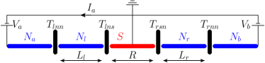
Figure 1: Schematic of the model.

The system can be described by a $4\times 4$ scattering matrix $s_{ij}^{\alpha\beta}$ where Latin indices run over the normal electrodes $a$ and $b$ and Greek indices over electrons $e$ and holes $h$. The scattering theory assumes that the superconductor is a reservoir of Cooper pairs, so the structure is implicitly a three-terminal one and the superconducting electrode is taken as grounded. The transformation of quasi-particles into Cooper pairs is taken into account by the correlation length $\xi(\omega)$ which sets the scale of the damping of the electron and hole wavefunctions in the superconductor.

The elements of the scattering matrix are evaluated from the BTK approachBTK1982 (see Appendix A). Here we do not use the Andreev approximation valid in the limit of zero energy where the electron and hole wavevectors are set to the Fermi wavelength, but instead keep the full expressions for the wavevectors. The calculation of the average current $I$ and current cross-correlations $S$ rely on the formulas derived by Anantram and Datta in Ref. AD1996, :

$$I_{i}=\frac{e}{h}\sum_{k\in\{a,b\}}\sum_{\alpha,\beta\in\{e,h\}}\mathrm{sgn}(\alpha)$$ (1)

$$\times\int dE\phantom{0}\left[\delta_{ik}\delta_{\alpha\beta}-\left|s_{ik}^{\alpha\beta}\right|^{2}\right]f_{k\beta}(E)$$

$$S_{ij}=\frac{2e^{2}}{h}\sum_{k,l\in\{a,b\}}\sum_{\alpha,\beta,\gamma,\delta\in\{e,h\}}\mathrm{sgn}(\alpha)\mathrm{sgn}(\beta)$$ (2)

$$\times\int dE\phantom{0}A_{k\gamma,l\delta}(i\alpha,E)A_{l\delta,k\gamma}(i\alpha,E)f_{k\gamma}(E)\left[1-f_{l\delta}(E)\right]$$

with $A_{k\gamma,l\delta}(i\alpha,E)=\delta_{ik}\delta_{il}\delta_{\alpha\gamma}\delta_{\alpha\delta}-s_{ik}^{\alpha\gamma\dagger}s_{il}^{\alpha\delta}$, $\mathrm{sgn}(\alpha=e)=1$ $\mathrm{sgn}(\alpha=h)=-1$, $f_{i\alpha}$ the occupancy factors for the electron and hole states in electrode $i$, given by the Fermi function where the chemical potential are the applied voltages $f_{ie}(E)=\left[1+\exp\left(\frac{E-V_{i}}{k_{B}T}\right)\right]^{-1}\xrightarrow[T\to 0]{}\theta(-E+V_{i})$, $f_{ih}(E)=\left[1+\exp\left(\frac{E+V_{i}}{k_{B}T}\right)\right]^{-1}\xrightarrow[T\to 0]{}\theta(-E-V_{i})$.

In this one-dimensional model, both current and noise are highly sensitive to the distances $L_{l}$, $R$, $L_{r}$ between the barriers: They oscillate as a function of these distances with a period equal to the Fermi wavelength $\lambda_{F}\ll L_{l},R,L_{r}$. In a higher-dimensional system with more than one transmission mode, the oscillations in the different modes are independent and are thus averaged out. Multidimensional behavior can be simulated qualitatively with a one-dimensional system by averaging all quantities over one oscillation period:

$$\overline{X}(L_{l},R,L_{r})$$ (3)

$$=\frac{1}{\lambda_{F}^{3}}\int_{L_{l}-\frac{\lambda_{F}}{2}}^{L_{l}+\frac{\lambda_{F}}{2}}dl_{l}\int_{R-\frac{\lambda_{F}}{2}}^{R+\frac{\lambda_{F}}{2}}dr\int_{L_{r}-\frac{\lambda_{F}}{2}}^{L_{r}+\frac{\lambda_{F}}{2}}dr\kern 2.0ptX(l_{l},r,l_{r}).$$

This procedure is appropriate to describe metallic systems. These averaged quantities are studied in section IV.

III Components of the Differential Conductance and the Differential Current Cross-Correlations

An electron, arriving from one of the normal metal reservoirs at the interface to the superconductor, can be: i) reflected as an electron (normal reflection (NR)), or ii) reflected as a hole (Andreev reflection (AR)), or iii) transmitted as an electron (elastic cotunneling (EC)) or iv) transmitted as a hole (crossed Andreev reflection (CAR)), and similarly for holes. The corresponding elements of the scattering matrix are for NR: $s_{aa}^{ee}$, $s_{aa}^{hh}$, $s_{bb}^{ee}$, $s_{bb}^{hh}$, AR: $s_{aa}^{eh}$, $s_{aa}^{he}$, $s_{bb}^{eh}$, $s_{bb}^{he}$, EC: $s_{ab}^{ee}$, $s_{ab}^{hh}$, $s_{ba}^{ee}$, $s_{ba}^{hh}$, and CAR: $s_{ab}^{eh}$, $s_{ab}^{he}$, $s_{ba}^{eh}$, $s_{ba}^{he}$.

The current in electrode $N_{a}$ given by Eq. (1) can naturally be divided into AR, CAR and EC contributions (the unitarity of the scattering matrix has been used):

$$I_{a}=\frac{|e|}{h}\int\mathrm{d}E \underbrace{\left[\left(|s_{aa}^{eh}(E)|^{2}+|s_{aa}^{he}(E)|^{2}\right)(f_{ae}(E)-f_{ah}(E))\right.}_{\text{local Andreev reflection}}$$

$$+ \underbrace{|s_{ab}^{ee}(E)|^{2}(f_{ae}(E)-f_{be}(E))+|s_{ab}^{hh}(E)|^{2}(f_{bh}(E)-f_{ah}(E))}_{\text{elastic cotunneling}}$$

$$+ \underbrace{\left.|s_{ab}^{eh}(E)|^{2}(f_{ae}(E)-f_{bh}(E))+|s_{ab}^{he}(E)|^{2}(f_{be}(E)-f_{ah}(E))\right]}_{\text{crossed Andreev reflection}}.$$ (4)

In the following, we focus on i) the differential conductance in the symmetrical case where $V_{a}=V_{b}=V$ and the current $I_{a}$ is differentiated with respect to $V$, and ii) the differential nonlocal conductance in the asymmetrical case where $V_{a}=0$ and the current $I_{a}$ is differentiated with respect to $V_{b}$. In the zero temperature limit, only the nonlocal processes, CAR and EC, contribute to the nonlocal conductance:

$$\left.\frac{\partial I_{a}}{\partial V_{b}}\right|_{V_{a}=0}=\underbrace{-\frac{e^{2}}{h}\left[|s_{ab}^{ee}(|e|V_{b})|^{2}+|s_{ab}^{hh}(-|e|V_{b})|^{2}\right]}_{\text{elastic cotunneling}}+\underbrace{\frac{e^{2}}{h}\left[|s_{ab}^{eh}(-|e|V_{b})|^{2}+|s_{ab}^{he}(|e|V_{b})|^{2}\right]}_{\text{crossed Andreev reflection}},$$ (5)

while the symmetric case contains local Andreev reflection and crossed Andreev reflection:

$$\left.\frac{\partial I_{a}}{\partial V}\right|_{V_{a}=V_{b}=V}= \underbrace{\frac{e^{2}}{h}\left[\left(|s_{aa}^{eh}(|e|V)|^{2}+|s_{aa}^{he}(|e|V)|^{2}\right)+\left(|s_{aa}^{eh}(-|e|V)|^{2}+|s_{aa}^{he}(-|e|V)|^{2}\right)\right]}_{\text{local Andreev reflection}}$$

$$+ \underbrace{\frac{e^{2}}{h}\left[\left(|s_{ab}^{eh}(|e|V)|^{2}+|s_{ab}^{he}(|e|V)|^{2}\right)+\left(|s_{ab}^{eh}(-|e|V)|^{2}+|s_{ab}^{he}(-|e|V)|^{2}\right)\right]}_{\text{crossed Andreev reflection}}$$ (6)

Let us now perform a similar analysis for the current cross-correlations. We study only the zero temperature limit, where $f_{k\gamma}(E)[1-f_{l\delta}(E)]$ is zero if $k=l$ and $\gamma=\delta$ and the current cross-correlations are:

$$S_{ab}(T=0)=\frac{2e^{2}}{h}\sum_{k,l\in\{a,b\}}\sum_{\alpha,\beta,\gamma,\delta\in\{e,h\}}\mathrm{sgn}(\alpha)\mathrm{sgn}(\beta)\int dEs_{ak}^{\alpha\gamma\dagger}s_{al}^{\alpha\delta}s_{bl}^{\beta\delta\dagger}s_{bk}^{\beta\gamma}f_{k\gamma}(E)[1-f_{l\delta}(E)]$$ (7)

Every summand in $S_{ab}$ contains the product of four elements of the scattering matrix. As pointed out in Refs. ML1992, ; Buettiker1990, , in difference to the situation for the current, it is impossible to combine those matrix elements to absolute squares. Let us now sort out and classify the contributions of the noise as we did above for the current. We find that no summand consists of only one kind of elements of the scattering matrix. Every element consists of two local elements (NR or AR ) and two nonlocal elements (CAR or EC) (see Appendix B). Either the two local elements and the two nonlocal elements are identical, that gives the components EC-NR, CAR-NR, EC-AR, CAR-AR, or all four matrix elements belong to different categories and we will call these summands MIXED. Sometimes, it is useful to divide MIXED further as a function of its voltage dependence. As the formulas for the current cross correlations are lengthy, they are relegated into Appendix B.

Examination of these expressions allows an interpretation of the various components. First, EC-NR does not involve any Andreev scattering and corresponds to quasiparticle fluctuations across the double $NSN$ barrier. Second, CAR-NR involves two amplitudes for electron-hole scattering across $NSN$ (Crossed Andreev) and two normal scattering amplitudes. This process tracks fluctuations of the current of split Cooper pairs emitted in- or absorbed by $S$. Third, EC-AR involves two local Andreev scattering amplitudes and propagation of a pair of quasiparticles in $S$. It thus reflects the fluctuations of pairs back and forth across the $NSN$ double interface. Fourth, CAR-AR involves two crossed Andreev and two normal Andreev amplitudes. This process which amounts to splitting two pairs from $S$ is usually weak. Fifth, mixed processes can be analyzed in the same fashion, they involve a combination of split pair and quasiparticle crossing fluctuations.

For the interpretation of current cross-correlations, the global sign plays an important role. Later on, the differential cross-correlation $\partial S_{ab}/\partial V_{a,b}$ will be plotted. For positive applied bias voltages, this quantity has the same sign as the current cross-correlations. For negative applied voltages current, cross-correlations and differential current cross-correlations have opposite signs. To avoid confusion, we only show pictures of the differential current cross-correlations calculated for positive bias voltages (and thus negative energies $E=-|e|V$). Due to the electron-hole symmetry of the model, differential current cross-correlations calculated for negative bias voltages are up to a global sign identical to the ones calculated at positive bias voltage. For small bias voltages, current cross-correlations depend linearly on voltage. Thus, current cross-correlations and differential current cross-correlations show the same qualitative behavior if studied as a function of the interface transparency or the distance between barriers.

In Ref. FFM2010, , we performed a similar analysis of current cross-correlations in terms of Green’s functions for a NSN structure. For the relations between these two classifications see Appendix C. Bignon et al. bignon have studied current cross-correlations in the tunneling limit. They find that noise measurements in the tunneling limit can give access to the CAR and EC contribution of the current. We have just seen, that at least two processes are involved in every component of noise, but the contributions of noise they calculate fall into the categories EC-NR and CAR-NR. In the tunneling limit, the NR contribution is very close to one, therefore what remains is very similar to the current contributions. In what follows, more generally, the CAR-NR component provides the diagnosis of Cooper pair splitting.

IV Results

IV.1 Positive Cross-Correlations without CAR

If a CAR process is interpreted as the splitting of a Cooper pair into two electrons leaving the superconductor in different electrodes, positive cross-correlations are its logical consequence. However, the CAR process is not the only one which can lead to positive cross-correlations. Let us investigate in more detail the influence of the different processes on the current cross-correlations in a NSN-system, i. e. in a system without the additional barriers in the normal conducting electrodes.

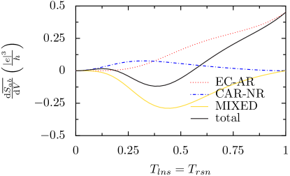
Figure 2: Averaged differential current cross-correlations for a symmetrical biased ($V=V_{a}=V_{b}\ll\Delta/|e|$) NSN-system as a function of the transparency of the interfaces $T_{lns}=T_{rsn}$. The positive cross-correlations at high interface transparency are due to the EC-AR process, represented by a dotted line.

The black line in Fig. 2 shows the averaged differential current cross-correlations for symmetric bias ($V=V_{a}=V_{b}$). The total current cross-correlations have already been published in Ref. FFM2010, , but here, Fig. 2 shows in addition the different parts which contribute to the total current cross-correlations. The total cross-correlations are positive for high interface transparencies and for low interface transparencies. As we have already argued in Ref. FFM2010, , the positive cross-correlations at high interface transparencies are not due to CAR : only processes which conserve momentum can occur, since there are no barriers which can absorb momentum. CAR processes do not conserve momentum: if e.g. an electron arrives from the left-hand side carrying momentum $k_{F}$, the hole that leaves at the right hand side carries momentum $-k_{F}$. As the cross-correlations do not tend to zero even for very high transparencies, they cannot be due do CAR. Indeed, if we plot the different components of the noise introduced in the last section separately, we see that the positive current cross-correlations at high interface transparencies have a different origin: a large positive EC-AR contribution, thus correlated pair fluctuations without pair splitting. But positive current cross-correlations at low interface transparencies are a consequence of a large CAR-NR component and therefore a consequence of CAR processes.

We can put the contributions to the current cross-correlations into two categories with respect to their sign, which is independent of the interface transparency. EC-NR, CAR-AR, MIXED2 and MIXED4 carry a negative sign, CAR-NR, EC-AR, MIXED1 and MIXED3 carry a positive sign. The current can either be carried by electrons $I^{e}$ or by holes $I^{h}$. The sign of the different contributions to the current cross-correlations depends on whether only currents of the same carrier type are correlated AD1996 ($\langle\Delta\hat{I}_{a}^{e}\Delta\hat{I}_{b}^{e}\rangle$+$\langle\Delta\hat{I}_{a}^{h}\Delta\hat{I}_{b}^{h}\rangle+a\leftrightarrow b$), which is the case for EC-NR, CAR-AR, MIXED2 and MIXED4 and leads to a negative sign; or whether electron currents are correlated with hole currents ($\langle\Delta\hat{I}_{a}^{e}\Delta\hat{I}_{b}^{h}\rangle$+$\langle\Delta\hat{I}_{a}^{h}\Delta\hat{I}_{b}^{e}\rangle+a\leftrightarrow b$), which is the case for CAR-NR, EC-AR, MIXED1 and MIXED3 and leads to a positive sign. In purely normal conducting systems, the electron and hole currents are uncorrelated, only correlations of the same carrier type contribute to the current cross-correlation and lead to a negative sign. The sign of the total current cross-correlations is a consequence of the relative strength of the different parts of the current cross-correlations, which depends on the interface transparency.

IV.2 Multiple Barriers

In the last paragraph, we showed that positive cross-correlations due to CAR can only be found in the tunneling regime, where the signals are quite weak. The conductance over an NS-tunnel junction can be amplified for a “dirty“ normal conductor containing a large number of non-magnetic impurities, where transport is diffusive, by an effect called reflectionless tunneling reflectionlesstunnexpt ; reflectionlesstunntheo , yielding an excess of conductance at low energy. It is thus natural to ask if a similar effect could also enhance conductance and current cross-correlations in a three terminal NSN-structure. To answer this question within the scattering approach, we use the model of Melsen and Beenakker MB1994 where the disordered normal conductor is replaced by a normal conductor with an additional tunnel barrier leading to an NNS structure. Duhot and Mélin duhotmelin have studied the influence of additional barriers on the nonlocal conductance in three terminal NSN-structures. They indeed find that two symmetric additional barriers enhance the nonlocal conductance. A similar result is obtained by quasiclassical methods in Ref. ZaikinPRL, .

First, let us get a deeper understanding of the result of Ref. duhotmelin, by calculating the AR, CAR and EC components of the current separately. Afterwards, we will study the influence of additional barriers on the current cross-correlations.

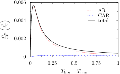
a) b)

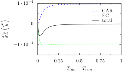
Figure 3: Averaged differential conductance in the limit of zero energy in a) the symmetrical bias situation $V_{a}=V_{b}\ll\Delta/|e|$ and b) in the asymmetrical case $V_{a}=0$, $V_{b}\ll\Delta/|e|$ for a superconducting electrode much shorter than the coherence length ($R=0.25\xi$) as a function of the transparencies of the additional barriers $T_{lnn}=T_{rnn}$. The barriers next to the superconductor are in the tunnel regime ($T_{lns}=T_{rsn}=0.01$).

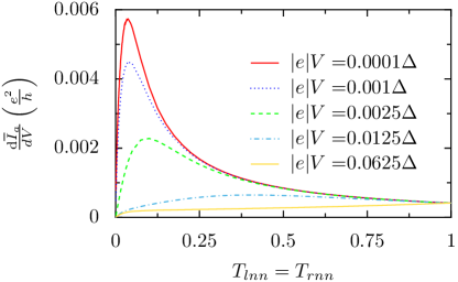
a) b)

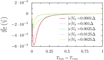
Figure 4: Total averaged differential conductance, as in Fig. 3 but at different energies.

Fig. 3 shows the averaged conductance in the symmetrical bias situation $V_{a}=V_{b}\ll\Delta/|e|$ and in the asymmetrical voltage case $V_{a}=0$, $V_{b}\ll\Delta/|e|$ for a superconducting electrode much shorter than the coherence length ($R=0.25\xi$). The sum of the AR, CAR and EC components, traced in black, features in both cases an extremum. Yet, examining at the behavior of these components, we see that they arise from different mechanisms. Let us first have a look at the symmetrically biased case. Without the additional barriers, i.e. in the limit $T_{lnn}=T_{rnn}\to 1$, the contributions of AR and CAR are similar in magnitude. The EC component is completely suppressed, since it is proportional to the difference of the applied voltages. The introduction of two additional barriers increases the AR component up to a factor 30. The shape of the curves is similar to the one of the NNS structure derived analytically by Melsen and Beenakker MB1994 , which can be exactly recovered by increasing the length of the superconducting electrode far beyond the coherence length. However, the CAR curve stays almost constant over a wide range of values of barrier strength of the additional barriers, and it eventually vanishes when the transparencies go to zero.

In the asymmetrical voltage case $V_{a}=0$, the AR component is zero as it is proportional to the local voltage $V_{a}$. Like in the first case, the additional barriers have little influence on the CAR component, except for the fact that it obviously tends to zero for vanishing transparency. Over a wide range of barrier strength values, lowest order tunneling prevails, and the EC component is identical in amplitude, but opposite in sign to the CAR component falci . For small $T_{lnn}=T_{rnn}$ values the EC component displays a small extremum, but it is much less pronounced than the maximum of the AR component of the first case. The CAR component, on the other hand, does not show any extremum.

In the limit $T_{lnn}=T_{rnn}\to 1$, the EC component tends more slowly to zero than the CAR component which as a consequence yields a maximum in the absolute value of the total conductance, dominated by EC. The fact that the conductance maxima in the symmetrical bias case and in the asymmetrical bias case have different origins can also be illustrated by studying their energy dependence, depicted in Fig. 4: The enhancement of the AR component of the conductance in the symmetrical biased case disappears completely with increasing bias voltage, as expected for a zero-bias anomaly. On the contrary, the extremum of the conductance in the asymmetrical biased case decreases slightly with increasing bias voltage, but only up to a certain voltage value, then it saturates.

Why is the AR component enhanced by the additional barriers, but not the EC or CAR components? Reflectionless tunneling occurs because the electrons and holes resonate inside the double barrier and have therefore a higher probability to enter the superconductor at low energy, despite phase-averaging. In the AR case the incoming electron and the leaving hole may encounter the same scattering path. On the contrary the EC and CAR process, the incoming particle and the leaving particle encounter different scattering path. The energy dependence of the conductance enhancement of the AR component is consistent with reflectionless tunneling which occurs at low bias voltage. At higher bias voltage, electrons and holes have different wavevectors and the reflectionless tunneling peak disappears. The integrals over the phases between the additional barriers on the left- and on the right-hand side have, of course, been taken independently. There is no reason to think that the channel mixing, which is emulated by the integrals, on the left- and on the right-hand side are coupled. To verify this scenario, let us couple the two integrals in an gedankenexperiment. We set the distance $L_{l}$ between the two left-hand side barriers to be equal to the distance $L_{r}$ between the two right-hand side barriers and perform only one integral over $L=L_{l}=L_{r}$. The result is shown in Fig. 5. Now, the CAR and the EC component are also enhanced by a large factor. Yet, the increase of the EC component is larger than the one of the CAR component, and EC still dominates the nonlocal conductance, like for a transparent $NSN$ structure.

To sum up the above analysis of the conductance enhancement by disorder, we showed that the crossed processes CAR and EC cannot be amplified but by an irrealistic correlation between disorder on the two sides of the NSN structure. Comparing qualitatively with the different approach of Ref. ZaikinPRL, , we also find an enhancement of the crossed conductance (Fig. 3b), which is not due to any marked maximum in CAR or EC components. Having the sign of EC, it cannot be interpreted in terms of enhanced Cooper pair splitting.

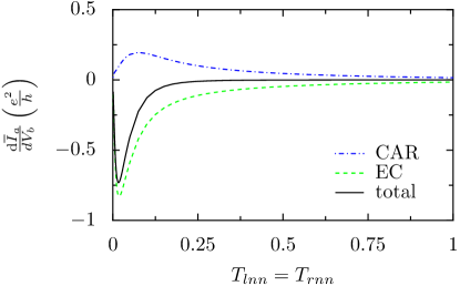
Figure 5: Effect of correlated averaging in the asymmetrical case with coupled integrals $T_{lns}=T_{rsn}=0.01$, $R=0.25\xi$: Now, also the EC and the CAR component are enhanced by reflectionless tunneling.

Let us turn back to independent averaging and consider the current cross-correlations. The results are shown in Fig. 6. In the symmetrical bias case, similarly to Fig. 3a, the additional barriers do not lead to an enhancement of the signal. The noise is dominated by the CAR-NR component, featuring Cooper pair splitting and, as we have seen above, CAR is not influenced by reflectionless tunneling. The EC-AR component, on the other hand, is amplified by the additional barriers, because the AR amplitude describing a local process is amplified. This leads to a small shoulder in the total cross-correlations. But since we are in the tunnel regime and the leading order of CAR-NR is $T^{2}$ while the leading order of EC-AR is $T^{4}$, the influence of the EC-AR-component is too small to lead to a global maximum.

In the asymmetrical bias case $V_{a}=0,V_{b}\ll\Delta/|e|$, on the other hand, the additional barriers weakly enhance the signal. But the cross-correlations are dominated by EC-NR and are therefore negative, and they do not feature Cooper pair splitting. In conclusion, in a phase-averaged system, additional barriers only enhance the AR-component, a local process. It cannot help to amplify nonlocal signals. Again, positive cross-correlations signalling Cooper pair splitting are only encountered in the tunneling regime. This conclusion is contrary to the interpretation of the quasiclassical theory given in Ref. ZaikinPRBnoise, .

a)
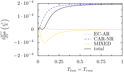
b)

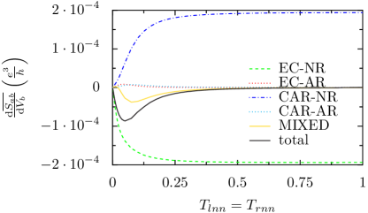
Figure 6: Averaged differential current cross-correlations in a) the symmetrical bias situation $V_{a}=V_{b}\ll\Delta/|e|$ and b) the asymmetrical bias case $V_{a}=0$, $V_{b}\ll\Delta/|e|$ for a superconducting electrode shorter than the coherence length ($R=0.25\xi$) as a function of the transparencies of the additional barriers $T_{lnn}=T_{rnn}$. The barriers next to the superconductor are in the tunnel regime ($T_{lns}=T_{rsn}=0.01$).

V Conclusion

We have found that at high transparency, crossed processes are dominated by electron transmission and that positive cross-correlations in this range of interface transparency are not due to Cooper pair splitting. Instead, for symmetrical voltages, they originate from correlated fluctuations of Cooper pairs from the superconductor to both metallic contacts and vice-versa. Cooper pair splitting in the tunnel regime cannot be enhanced with additional barriers by a process similar to reflectionless tunneling, if an average (here, over the interbarrier lengths) has to be performed, mimicking disorder landscapes which are uncorrelated on the two sides of the set-up. In analogy, one expects that the same conclusion holds if one uses diffusive normal metals. These conclusions are important for settling future experimental programs. Positive cross-correlations might well be observed at high transparency, but they are not a signature of Cooper pair splitting. They are not related to spatially separated spin-entangled pairs. Conductance and cross-correlation measurements with controlled and tunable interface transparencies would be very useful, and may be attempted for instance in carbon nanotubes junctions. Finally, a cross-over to negative current cross-correlations for a highly transparent NSN junction biased above the gap is expected. Its theoretical description is more involved, because it requires taking nonequilibrium effects such as charge imbalance imb1 ; imb2 ; imb3 into account. A starting point for those calculations can be found in Ref. Melin-Bergeret-Yeyati, .

Appendix A Details on the scattering approach

The elements $s_{ij}^{\alpha\beta}$ of the scattering matrix are calculated within the BTK approachBTK1982 : Two-component wavefunctions, where the upper component describes electrons and the lower components holes, are matched at the interfaces and the coefficients of the resulting system of equations give the elements of the scattering matrix.

In the normal conductors the the wavefunctions are plane waves with wavevectors close to the Fermi wavevector $\hbar k_{F}=\sqrt{2m\mu}$. The wavevector for electrons reads $\hbar q^{+}=\sqrt{2m}\sqrt{\mu+E}$, the one for holes $\hbar q^{+}=\sqrt{2m}\sqrt{\mu-E}$. In the superconductor, the wavefunction has to obey the Bogoliubov-De Gennes equation, where the superconducting gap is supposed to be a positive constant inside the superconductor and zero outside of it. This is achieved by modifying the amplitudes of the wavefunction in the superconductor with the coherence factors $u_{E}$ and $v_{E}$ which read for energies smaller than the gap ($E<\Delta$):

$$u_{E}=\frac{1}{\sqrt{2}}\sqrt{1+\frac{i\sqrt{\Delta^{2}-E^{2}}}{E}},\phantom{000}v_{E}=\frac{1}{\sqrt{2}}\sqrt{1-\frac{i\sqrt{\Delta^{2}-E^{2}}}{E}}$$ (8)

and by using for quasi-particles proportional to $\begin{pmatrix}u_{E}\\ v_{E}\end{pmatrix}$ the wavevector $\hbar k^{+}=\sqrt{2m}\sqrt{\mu+i\sqrt{\Delta^{2}-E^{2}}}$ and for quasi-particles proportional to $\begin{pmatrix}v_{E}\\ u_{E}\end{pmatrix}$ the wavevector $\hbar k^{-}=\sqrt{2m}\sqrt{\mu-i\sqrt{\Delta^{2}-E^{2}}}$.

For example, the wavefunctions for an electron incoming from electrode N_a take the form

$$\psi_{\mathrm{N}_{a}}(x) =\begin{pmatrix}1\\ 0\end{pmatrix}\left(1\phantom{0}e^{iq^{+}x}+s^{ee}_{aa}\phantom{0}e^{-iq^{+}x}\right)+\begin{pmatrix}0\\ 1\end{pmatrix}\left(s^{he}_{aa}\phantom{0}e^{iq^{-}x}+0\phantom{0}e^{-iq^{-}x}\right),$$ (9)

$$\psi_{\mathrm{N}_{l}}(x) =\begin{pmatrix}1\\ 0\end{pmatrix}\left(c_{1}\phantom{0}e^{iq^{+}x}+c_{2}\phantom{0}e^{-iq^{+}(x-L_{l})}\right)+\begin{pmatrix}0\\ 1\end{pmatrix}\left(c_{3}\phantom{0}e^{iq^{-}x}+c_{4}\phantom{0}e^{-iq^{-}(x-L_{l})}\right),$$ (10)

$$\psi_{\mathrm{S}}(x) =\begin{pmatrix}u_{E}\\ v_{E}\end{pmatrix}\left(c_{5}\phantom{0}e^{ik^{+}(x-L_{l})}+c_{6}\phantom{0}e^{-ik^{+}(x-L_{l}-R)}\right)$$

$$+\begin{pmatrix}v_{E}\\ u_{E}\end{pmatrix}\left(c_{7}\phantom{0}e^{-ik^{-}(x-L_{l}}+c_{8}\phantom{0}e^{ik^{-}(x-L_{l}-R)}\right),$$ (11)

$$\psi_{\mathrm{N}_{r}}(x) =\begin{pmatrix}1\\ 0\end{pmatrix}\left(c_{9}\phantom{0}e^{iq^{+}(x-L_{l}-R)}+c_{10}\phantom{0}e^{-iq^{+}(x-L_{l}-R-L_{r})}\right)$$

$$+\begin{pmatrix}0\\ 1\end{pmatrix}\left(c_{11}\phantom{0}e^{iq^{-}(x-L_{l}-R)}+c_{12}\phantom{0}e^{-iq^{-}(x-L_{l}-R-L_{r})}\right),$$ (12)

$$\psi_{\mathrm{N}_{b}}(x) =\begin{pmatrix}1\\ 0\end{pmatrix}\left(s^{e,e}_{b,a}\phantom{0}e^{iq^{+}(x-L_{l}-R-L_{r})}+0\phantom{0}e^{-iq^{+}(x-L_{l}-R-L_{r})}\right)$$

$$+\begin{pmatrix}0\\ 1\end{pmatrix}\left(0\phantom{0}e^{iq^{-}(x-L_{l}-R)}+s^{h,e}_{b,a}\phantom{0}e^{-iq^{-}(x-L_{l}-R-L_{r})}\right)$$ (13)

n in the sections N_a, N_l, S, N_r, and N_b respectively [see Fig. 1] and give access to the scattering matrix elements $s^{e,e}_{a,a}$, $s^{h,e}_{a,a}$, $s^{h,e}_{b,a}$ and $s^{e,e}_{b,a}$. The remaining elements of the scattering matrix can be obtained from the other possible scattering processes i.e. a hole incoming from electrode N_a, an electron/hole incoming from electrode N_b.

The interfaces are modeled by $\delta$-potentials $V(x)=Z\hbar v_{F}\delta(x)$, where the BTK parameter $Z$ is connected to the interface transparency $T$ by $T=(1+Z^{2})^{-1}$. The elements of the scattering matrix can be determined and the constants $c_{i}$ eliminated using the continuity of the wavefunctions at the interfaces [$\psi_{N_{a}}(0)=\psi_{N_{l}}(0)$ etc.] and the boundary condition for the derivatives [$\psi_{N_{l}}^{\prime}(0)-\psi_{N_{a}}^{\prime}(0)=Z\hbar v_{F}\psi_{a}(0)$ etc.] at every interface.

In simple cases, i. e. for only two or three sections and in the limit of zero energy, the system of equations giving the scattering matrix elements can be solved analytically (see FFM2010 ), but in the present case of five sections the expressions become so unhandy that the equations are solved numerically.

Appendix B Components of Current Cross Correlations

Components of the current cross-correlations:

$$S_{ab}(T=0,V_{a},V_{b})=\frac{2e^{2}}{h}\int dE\phantom{0}\biggr{(}$$

$$\left.\begin{aligned} &2\Re\left[s_{ab}^{ee}s_{ba}^{ee}s_{aa}^{ee\dagger}s_{bb}^{ee\dagger}\right](\theta(|e|V_{a}-E)-2\theta(|e|V_{a}-E)\theta(|e|V_{b}-E)+\theta(|e|V_{b}-E))\\ +&2\Re\left[s_{ab}^{hh}s_{ba}^{hh}s_{aa}^{hh\dagger}s_{bb}^{hh\dagger}\right](\theta(-|e|V_{a}-E)-2\theta(-|e|V_{a}-E)\theta(-|e|V_{b}-E)+\theta(-|e|V_{b}-E))\end{aligned}\right\}{EC-NR}$$

$$\left.\begin{aligned} +&2\Re\left[s_{ba}^{eh}s_{ab}^{he}s_{aa}^{hh\dagger}s_{bb}^{ee\dagger}\right](-\theta(-|e|V_{a}-E)+2\theta(-|e|V_{a}-E)\theta(|e|V_{b}-E)-\theta(|e|V_{b}-E))\\ +&2\Re\left[s_{ab}^{eh}s_{ba}^{he}s_{aa}^{ee\dagger}s_{bb}^{hh\dagger}\right](-\theta(|e|V_{a}-E)+2\theta(|e|V_{a}-E)\theta(-|e|V_{b}-E)-\theta(-|e|V_{b}-E))\\ \end{aligned}\right\}{CAR-NR}$$

$$\left.\begin{aligned} +&2\Re\left[s_{ab}^{hh}s_{ba}^{ee}s_{bb}^{eh\dagger}s_{aa}^{he\dagger}\right](-\theta(|e|V_{a}-E)+2\theta(|e|V_{a}-E)\theta(-|e|V_{b}-E)-\theta(-|e|V_{b}-E))\\ +&2\Re\left[s_{ab}^{ee}s_{ba}^{hh}s_{aa}^{eh\dagger}s_{bb}^{he\dagger}\right](-\theta(-|e|V_{a}-E)+2\theta(-|e|V_{a}-E)\theta(|e|V_{b}-E)-\theta(|e|V_{b}-E))\\ \end{aligned}\right\}{EC-AR}$$

$$\left.\begin{aligned} +&2\Re\left[s_{ba}^{he}s_{ab}^{he}s_{aa}^{he\dagger}s_{bb}^{he\dagger}\right](\theta(|e|V_{a}-E)-2\theta(|e|V_{a}-E)\theta(|e|V_{b}-E)+\theta(|e|V_{b}-E))\\ +&2\Re\left[s_{ab}^{eh}s_{ba}^{eh}s_{aa}^{eh\dagger}s_{bb}^{eh\dagger}\right](\theta(-|e|V_{a}-E)-2\theta(-|e|V_{a}-E)\theta(-|e|V_{b}-E)+\theta(-|e|V_{b}-E))\\ \end{aligned}\right\}{CAR-AR}$$

$$\left.\begin{aligned} +&2\Re\left[s_{ab}^{eh}s_{ba}^{hh}s_{bb}^{hh\dagger}s_{aa}^{eh\dagger}+s_{ab}^{hh}s_{ba}^{eh}s_{aa}^{hh\dagger}s_{bb}^{eh\dagger}\right](-\theta(-|e|V_{a}-E)+2\theta(-|e|V_{a}-E)\theta(-|e|V_{b}-E)-\theta(-|e|V_{b}-E))\\ +&2\Re\left[s_{ab}^{ee}s_{ba}^{he}s_{aa}^{ee\dagger}s_{bb}^{he\dagger}+s_{ba}^{ee}s_{ab}^{he}s_{bb}^{ee\dagger}s_{aa}^{he\dagger}\right](-\theta(|e|V_{a}-E)+2\theta(|e|V_{a}-E)\theta(|e|V_{b}-E)-\theta(|e|V_{b}-E))\\ \end{aligned}\right\}{MIXED1}$$

$$\left.\begin{aligned} +&2\Re\left[s_{ab}^{ee}s_{ba}^{eh}s_{bb}^{ee\dagger}s_{aa}^{eh\dagger}+s_{ba}^{hh}s_{ab}^{he}s_{aa}^{hh\dagger}s_{bb}^{he\dagger}\right](\theta(-|e|V_{a}-E)-2\theta(-|e|V_{a}-E)\theta(|e|V_{b}-E)+\theta(|e|V_{b}-E))\\ +&2\Re\left[s_{ab}^{eh}s_{ba}^{ee}s_{aa}^{ee\dagger}s_{bb}^{eh\dagger}+s_{ab}^{hh}s_{ba}^{he}s_{bb}^{hh\dagger}s_{aa}^{he\dagger}\right](\theta(|e|V_{a}-E)-2\theta(|e|V_{a}-E)\theta(-|e|V_{b}-E)+\theta(-|e|V_{b}-E))\\ \end{aligned}\right\}{MIXED2}$$

$$\left.\begin{aligned} +&2\Re\left[s_{aa}^{hh}s_{ba}^{ee}s_{ba}^{eh\dagger}s_{aa}^{he\dagger}+s_{aa}^{ee}s_{ba}^{hh}s_{ba}^{he\dagger}s_{aa}^{eh\dagger}\right](-\theta(|e|V_{a}-E)+2\theta(|e|V_{a}-E)\theta(-|e|V_{a}-E)-\theta(-|e|V_{a}-E))\\ \end{aligned}\right\}{MIXED3a}$$

$$\left.\begin{aligned} +&2\Re\left[s_{ab}^{eh}s_{bb}^{he}s_{ab}^{ee\dagger}s_{bb}^{hh\dagger}+s_{ab}^{hh}s_{bb}^{ee}s_{ab}^{he\dagger}s_{bb}^{eh\dagger}\right](-\theta(|e|V_{b}-E)+2\theta(|e|V_{b}-E)\theta(-|e|V_{b}-E)-\theta(-|e|V_{b}-E))\\ \end{aligned}\right\}{MIXED3b}$$

$$\left.\begin{aligned} +&2\Re\left[s_{aa}^{eh}s_{ba}^{ee}s_{aa}^{ee\dagger}s_{ba}^{eh\dagger}+s_{ba}^{hh}s_{aa}^{he}s_{aa}^{hh\dagger}s_{ba}^{he\dagger}\right](\theta(|e|V_{a}-E)-2\theta(|e|V_{a}-E)\theta(-|e|V_{a}-E)+\theta(-|e|V_{a}-E))\\ \end{aligned}\right\}{MIXED4a}$$

$$\left.\begin{aligned} +&2\Re\left[s_{ab}^{ee}s_{ab}^{eh}s_{bb}^{ee\dagger}s_{ab}^{eh\dagger})+s_{ab}^{eh}s_{bb}^{he}s_{bb}^{hh\dagger}s_{ab}^{he\dagger})\right](\theta(|e|V_{b}-E)-2\theta(|e|V_{b}-E)\theta(-|e|V_{b}-E)+\theta(-|e|V_{b}-E))\biggl{)}\\ \end{aligned}\right\}{MIXED4b}$$

Differential current cross-correlations in the nonlocal conductance setup:

$$\frac{\mathrm{d}S_{ab}(T=0,V_{a}=0,V_{b})}{\mathrm{d}V_{b}}=\left.\right.\frac{2|e|^{3}}{h}\mathrm{sgn}(V_{b})\biggl{(}$$

$$\left.\begin{aligned} &\phantom{+}2\Re\left[s_{ab}^{ee}(|e|V_{b})s_{ba}^{ee}(|e|V_{b})s_{aa}^{ee\dagger}(|e|V_{b})s_{bb}^{ee\dagger}(|e|V_{b})\right]+2\Re\left[s_{ab}^{hh}(-|e|V_{b})s_{ba}^{hh}(-|e|V_{b})s_{aa}^{hh\dagger}(-|e|V_{b})s_{bb}^{hh\dagger}(-|e|V_{b})\right]\\ \end{aligned}\right\}{EC-NR}$$

$$\left.\begin{aligned} -&2\Re\left[s_{ba}^{eh}(|e|V_{b})s_{ab}^{he}(|e|V_{b})s_{aa}^{hh\dagger}(|e|V_{b})s_{bb}^{ee\dagger}(|e|V_{b})\right]-2\Re\left[s_{ab}^{eh}(-|e|V_{b})s_{ba}^{he}(-|e|V_{b})s_{aa}^{ee\dagger}(-|e|V_{b})s_{bb}^{hh\dagger}(-|e|V_{b})\right]\\ \end{aligned}\right\}{CAR-NR}$$

$$\left.\begin{aligned} -&2\Re\left[s_{ab}^{ee}(|e|V_{b})s_{ba}^{hh}(|e|V_{b})s_{aa}^{eh\dagger}(|e|V_{b})s_{bb}^{he\dagger}(|e|V_{b})\right]-2\Re\left[s_{ab}^{hh}(-|e|V_{b})s_{ba}^{ee}(-|e|V_{b})s_{bb}^{eh\dagger}(-|e|V_{b})s_{aa}^{he\dagger}(-|e|V_{b})\right]\\ \end{aligned}\right\}{EC-AR}$$

$$\left.\begin{aligned} +&2\Re\left[s_{ba}^{he}(|e|V_{b})s_{ab}^{he}(|e|V_{b})s_{aa}^{he\dagger}(|e|V_{b})s_{bb}^{he\dagger}(|e|V_{b})\right]+2\Re\left[s_{ab}^{eh}(-|e|V_{b})s_{ba}^{eh}(-|e|V_{b})s_{aa}^{eh\dagger}(-|e|V_{b})s_{bb}^{eh\dagger}(-|e|V_{b})\right]\\ \end{aligned}\right\}{CAR-AR}$$

$$\left.\begin{aligned} -&2\Re\left[s_{ab}^{ee}(|e|V_{b})s_{ba}^{he}(|e|V_{b})s_{aa}^{ee\dagger}(|e|V_{b})s_{bb}^{he\dagger}(|e|V_{b})+s_{ba}^{ee}(|e|V_{b})s_{ab}^{he}(|e|V_{b})s_{bb}^{ee\dagger}(|e|V_{b})s_{aa}^{he\dagger}(|e|V_{b})\right]\\ -&2\Re\left[s_{ab}^{eh}(-|e|V_{b})s_{ba}^{hh}(-|e|V_{b})s_{bb}^{hh\dagger}(-|e|V_{b})s_{aa}^{eh\dagger}(-|e|V_{b})+s_{ab}^{hh}(-|e|V_{b})s_{ba}^{eh}(-|e|V_{b})s_{aa}^{hh\dagger}(-|e|V_{b})s_{bb}^{eh\dagger}(-|e|V_{b})\right]\\ \end{aligned}\right\}{MIXED1}$$

$$\left.\begin{aligned} +&2\Re\left[s_{ab}^{eh}(|e|V_{b})s_{ba}^{ee}(|e|V_{b})s_{aa}^{ee\dagger}(|e|V_{b})s_{bb}^{eh\dagger}(|e|V_{b})+s_{ab}^{hh}(|e|V_{b})s_{ba}^{he}(|e|V_{b})s_{bb}^{hh\dagger}(|e|V_{b})s_{aa}^{he\dagger}(|e|V_{b})\right]\\ +&2\Re\left[s_{ab}^{ee}(-|e|V_{b})s_{ba}^{eh}(-|e|V_{b})s_{bb}^{ee\dagger}(-|e|V_{b})s_{aa}^{eh\dagger}(-|e|V_{b})+s_{ba}^{hh}(-|e|V_{b})s_{ab}^{he}(-|e|V_{b})s_{aa}^{hh\dagger}(-|e|V_{b})s_{bb}^{he\dagger}(-|e|V_{b})\right]\\ \end{aligned}\right\}{MIXED2}$$

$$\left.\begin{aligned} -&2\Re\left[s_{ab}^{eh}(|e|V_{b})s_{bb}^{he}(|e|V_{b})s_{ab}^{ee\dagger}(|e|V_{b})s_{bb}^{hh\dagger}(|e|V_{b})+s_{ab}^{hh}(|e|V_{b})s_{bb}^{ee}(|e|V_{b})s_{ab}^{he\dagger}(|e|V_{b})s_{bb}^{eh\dagger}(|e|V_{b})\right]\\ -&2\Re\left[s_{ab}^{eh}(-|e|V_{b})s_{bb}^{he}(-|e|V_{b})s_{ab}^{ee\dagger}(-|e|V_{b})s_{bb}^{hh\dagger}(-|e|V_{b})+s_{ab}^{hh}(-|e|V_{b})s_{bb}^{ee}(-|e|V_{b})s_{ab}^{he\dagger}(-|e|V_{b})s_{bb}^{eh\dagger}(-|e|V_{b})\right]\\ \end{aligned}\right\}{MIXED3b}$$

$$\left.\begin{aligned} +&2\Re\left[s_{ab}^{ee}(|e|V_{b})s_{ab}^{eh}(|e|V_{b})s_{bb}^{ee\dagger}(|e|V_{b})s_{ab}^{eh\dagger}(|e|V_{b})+s_{ab}^{eh}(|e|V_{b})s_{bb}^{he}(|e|V_{b})s_{bb}^{hh\dagger}(|e|V_{b})s_{ab}^{he\dagger}(|e|V_{b})\right]\\ +&2\Re\left[s_{ab}^{ee}(-|e|V_{b})s_{ab}^{eh}(-|e|V_{b})s_{bb}^{ee\dagger}(-|e|V_{b})s_{ab}^{eh\dagger}(-|e|V_{b})+s_{ab}^{eh}(-|e|V_{b})s_{bb}^{he}(-|e|V_{b})s_{bb}^{hh\dagger}(-|e|V_{b})s_{ab}^{he\dagger}(-|e|V_{b})\right]\biggl{)}\\ \end{aligned}\right\}{MIXED4b}$$

Differential current cross-correlations in the symmetrical setup:

$$\frac{dS_{ab}(T=0,V_{a}+V,V_{b}=V)}{dV}=\frac{2|e|^{3}}{h}\mathrm{sgn}(|e|V)\phantom{0}\biggr{(}$$

$$\left.\begin{aligned} -&2\Re\left[s_{ba}^{eh}(|e|V)s_{ab}^{he}(|e|V)s_{aa}^{hh\dagger}(|e|V)s_{bb}^{ee\dagger}(|e|V)+s_{ab}^{eh}(|e|V)s_{ba}^{he}(|e|V)s_{aa}^{ee\dagger}(|e|V)s_{bb}^{hh\dagger}(|e|V)\right]\\ -&2\Re\left[s_{ba}^{eh}(-|e|V)s_{ab}^{he}(-|e|V)s_{aa}^{hh\dagger}(-|e|V)s_{bb}^{ee\dagger}(-|e|V)+s_{ab}^{eh}(-|e|V)s_{ba}^{he}(-|e|V)s_{aa}^{ee\dagger}(-|e|V)s_{hh}^{bb\dagger}(-|e|V)\right]\\ \end{aligned}\right\}{CAR-NR}$$

$$\left.\begin{aligned} -&2\Re\left[s_{ab}^{hh}(|e|V)s_{ba}^{ee}(|e|V)s_{bb}^{eh\dagger}(|e|V)s_{aa}^{he\dagger}(|e|V)+s_{ab}^{ee}(|e|V)s_{ba}^{hh}(|e|V)s_{aa}^{eh\dagger}(|e|V)s_{bb}^{he\dagger}(|e|V)\right]\\ -&2\Re\left[s_{ab}^{hh}(-|e|V)s_{ba}^{ee}(-|e|V)s_{bb}^{eh\dagger}(-|e|V)s_{aa}^{he\dagger}(-|e|V)+s_{ab}^{ee}(-|e|V)s_{ba}^{hh}(-|e|V)s_{aa}^{eh\dagger}(-|e|V)s_{bb}^{he\dagger}(-|e|V)\right]\\ \end{aligned}\right\}{EC-AR}$$

$$\left.\begin{aligned} +&2\Re\left[s_{ab}^{ee}(|e|V)s_{ba}^{eh}(|e|V)s_{bb}^{ee\dagger}(|e|V)s_{aa}^{eh\dagger}(|e|V)+s_{ba}^{hh}(|e|V)s_{ab}^{he}(|e|V)s_{aa}^{hh\dagger}(|e|V)s_{bb}^{he\dagger}(|e|V)\right]\\ +&2\Re\left[s_{ab}^{ee}(-|e|V)s_{ba}^{eh}(-|e|V)s_{bb}^{ee\dagger}(-|e|V)s_{aa}^{eh\dagger}(-|e|V)+s_{ba}^{hh}(-|e|V)s_{ab}^{he}(-|e|V)s_{aa}^{hh\dagger}(-|e|V)s_{bb}^{he\dagger}(-|e|V)\right]\\ +&2\Re\left[s_{ab}^{eh}(|e|V)s_{ba}^{ee}(|e|V)s_{aa}^{ee\dagger}(|e|V)s_{bb}^{eh\dagger}(|e|V)+s_{ab}^{hh}(|e|V)s_{ba}^{he}(|e|V)s_{bb}^{hh\dagger}(|e|V)s_{aa}^{he\dagger}(|e|V)\right]\\ +&2\Re\left[s_{ab}^{eh}(-|e|V)s_{ba}^{ee}(-|e|V)s_{aa}^{ee\dagger}(-|e|V)s_{bb}^{eh\dagger}(-|e|V)+s_{ab}^{hh}(-|e|V)s_{ba}^{he}(-|e|V)s_{bb}^{hh\dagger}(-|e|V)s_{aa}^{he\dagger}(-|e|V)\right]\\ \end{aligned}\right\}{MIXED2}$$

$$\left.\begin{aligned} -&2\Re\left[s_{aa}^{hh}(|e|V)s_{ba}^{ee}(|e|V)s_{ba}^{eh\dagger}(|e|V)s_{aa}^{he\dagger}(|e|V)+s_{aa}^{ee}(|e|V)s_{ba}^{hh}(|e|V)s_{ba}^{he\dagger}(|e|V)s_{aa}^{eh\dagger}(|e|V)\right]\\ -&2\Re\left[s_{aa}^{hh}(-|e|V)s_{ba}^{ee}(-|e|V)s_{ba}^{eh\dagger}(-|e|V)s_{aa}^{he\dagger}(-|e|V)+s_{aa}^{ee}(-|e|V)s_{ba}^{hh}(-|e|V)s_{ba}^{he\dagger}(-|e|V)s_{aa}^{eh\dagger}(-|e|V)\right]\\ \end{aligned}\right\}{MIXED3a}$$

$$\left.\begin{aligned} -&2\Re\left[s_{ab}^{eh}(|e|V)s_{bb}^{he}(|e|V)s_{ab}^{ee\dagger}(|e|V)s_{bb}^{hh\dagger}(|e|V)+s_{ab}^{hh}(|e|V)s_{bb}^{ee}(|e|V)s_{ab}^{he\dagger}(|e|V)s_{bb}^{eh\dagger}(|e|V)\right]\\ -&2\Re\left[s_{ab}^{eh}(-|e|V)s_{bb}^{he}(-|e|V)s_{ab}^{ee\dagger}(-|e|V)s_{bb}^{hh\dagger}(-|e|V)+s_{ab}^{hh}(-|e|V)s_{bb}^{ee}(-|e|V)s_{ab}^{he\dagger}(-|e|V)s_{bb}^{eh\dagger}(-|e|V)\right]\\ \end{aligned}\right\}{MIXED3b}$$

$$\left.\begin{aligned} +&2\Re\left[s_{aa}^{eh}(|e|V)s_{ba}^{ee}(|e|V)s_{aa}^{ee\dagger}(|e|V)s_{ba}^{eh\dagger}(|e|V)+s_{ba}^{hh}(|e|V)s_{aa}^{he}(|e|V)s_{aa}^{hh\dagger}(|e|V)s_{ba}^{he\dagger}(|e|V)\right]\\ +&2\Re\left[s_{aa}^{eh}(-|e|V)s_{ba}^{ee}(-|e|V)s_{aa}^{ee\dagger}(-|e|V)s_{ba}^{eh\dagger}(-|e|V)+s_{ba}^{hh}(-|e|V)s_{aa}^{he}(-|e|V)s_{aa}^{hh\dagger}(-|e|V)s_{ba}^{he\dagger}(-|e|V)\right]\\ \end{aligned}\right\}{MIXED4a}$$

$$\left.\begin{aligned} +&2\Re\left[s_{ab}^{ee}(|e|V)s_{ab}^{eh}(|e|V)s_{bb}^{ee\dagger}(|e|V)s_{ab}^{eh\dagger}(|e|V)+s_{ab}^{eh}(|e|V)s_{bb}^{he}(|e|V)s_{bb}^{hh\dagger}(|e|V)s_{ab}^{he\dagger}(|e|V)\right]\\ +&2\Re\left[s_{ab}^{ee}(-|e|V)s_{ab}^{eh}(-|e|V)s_{bb}^{ee\dagger}(-|e|V)s_{ab}^{eh\dagger}(-|e|V)+s_{ab}^{eh}(-|e|V)s_{bb}^{he}(-|e|V)s_{bb}^{hh\dagger}(-|e|V)s_{ab}^{he\dagger}(-|e|V)\right]\biggl{)}\\ \end{aligned}\right\}{MIXED4b}$$

Appendix C Relations between the noise classification in the BTK and in the Green’s functions approach

Scattering matrix	Green’s function
classification	classification
CAR-NR	CAR
EC-AR	$\mathrm{AR}\text{-}\overline{\mathrm{AR}}$
MIXED1, MIXED2	PRIME
EC-NR	EC
CAR-AR	AR-AR
MIXED3, MIXED4	MIXED

Table 1: Correspondences between the categories in the language of Green’s functions from FFM2010 and in the language of scattering matrix elements.

The elements of the scattering-matrix are connected to the retarded Green’s functions of the tight binding model studied in FFM2010 via

$$s_{ij}^{\alpha\beta}=i\delta_{ij}+2\pi t_{i}t_{j}\sqrt{\rho_{i}^{\alpha}}\sqrt{\rho_{j}^{\beta}}G_{ij\alpha\beta}^{R}$$ (14)

where $t_{i}$ is the transmission coefficient of the barrier $i$, $\rho_{i}^{\alpha}$ the density of electron or hole states of electrode $i$ and $G_{ij\alpha\beta}^{R}$ the Green’s function connecting the first site in the superconductor next to the electrode $j$ to the first site in the superconductor next to the electrode $i$.

Table 1 shows the correspondences between the categories in the language of Green’s functions and in the language of scattering matrix elements.

References

- (1) M. S. Choi, C. Bruder, and D. Loss, Phys. Rev. B 62, 13569 (2000); P. Recher, E. V. Sukhorukov, and D. Loss, Phys. Rev. B 63, 165314 (2001).
- (2) G.B. Lesovik, T. Martin, and G. Blatter, Eur. Phys. J. B 24, 287 (2001); N. M. Chtchelkatchev, G. Blatter, G. B. Lesovik, and T. Martin, Phys. Rev. B 66, 161320 (2002).
- (3) N. K. Allsopp, V. C. Hui, C. J. Lambert, and S. J. Robinson, J. Phys.: Condens. Matter 6, 10475 (1994).
- (4) J. M. Byers and M. E. Flatté, Phys. Rev. Lett. 74, 306 (1995).
- (5) J. Torrès and T. Martin, Eur. Phys. J. B 12, 319 (1999).
- (6) G. Deutscher and D. Feinberg, Appl. Phys. Lett. 76, 487 (2000).
- (7) G. Falci, D. Feinberg, and F. W. J. Hekking, Europhys. Lett. 54, 255 (2001).
- (8) R. Mélin and D. Feinberg, Eur. Phys. J. B 26, 101 (2002).
- (9) R. Mélin and D. Feinberg, Phys. Rev. B 70, 174509 (2004).
- (10) M. Büttiker, Phys. Rev. B 46, 12485 (1992).
- (11) G. Bignon, M. Houzet, F. Pistolesi, and F. W. J. Hekking, Europhys. Lett. 67, 110 (2004).
- (12) F.Taddei and R. Fazio, Phys. Rev. B 65, 075317 (2002).
- (13) J.P. Morten, D. Huertas-Hernando, W. Belzig, and A. Brataas, Phys. Rev. B 78, 224515 (2008).
- (14) M. P. Anantram and S. Datta, Phys. Rev. B 53, 16390 (1996).
- (15) A. Brinkman and A.A. Golubov, Phys. Rev. B 74, 214512 (2006).
- (16) D. Sánchez, R. López, P. Samuelsson, and M. Büttiker, Phys. Rev. B 68, 214501 (2003).
- (17) S. Russo, M. Kroug, T. M. Klapwijk, and A. F. Morpurgo, Phys. Rev. Lett. 95, 027002 (2005).
- (18) A. Levy Yeyati, F.S. Bergeret, A. Martín Rodero, and T.M. Klapwijk, Nature Phys. 3, 455 (2007).
- (19) B. Kaviraj, O. Coupiac, H. Courtois and F. Lefloch, Phys. Rev. Lett. 107, 077005 (2011)
- (20) R. Mélin, Phys. Rev. B 73, 174512 (2006).
- (21) S. Duhot and R. Mélin, Eur. Phys. J. B 53, 257 (2006).
- (22) J. P. Morten, A. Brataas, and W. Belzig, Phys. Rev. B74, 214510 (2006).
- (23) M. S. Kalenkov and A. D. Zaikin, Phys. Rev. B 75, 172503 (2007).
- (24) A. Freyn, M. Flöser and R. Mélin, Phys. Rev. B 82, 014510 (2010).
- (25) D. Beckmann, H. B. Weber, and H. v. Löhneysen, Phys. Rev. Lett. 93, 197003 (2004); P. Cadden-Zimansky and V. Chandrasekhar, Phys. Rev. Lett. 97, 237003 (2006); P. Cadden-Zimansky, Z. Jiang, and V. Chandrasekhar, New Journal of Physics 9, 116 (2007); P. Cadden-Zimansky, J. Wei and V. Chandrasekhar, Nature Physics 5, 393 (2009); T. Noh, S. Davis, and V. Chandrasekhar, Arxiv preprint arXiv:1210.8426.
- (26) L. Hofstetter, S. Csonka, J. Nygård, and C. Schönenberger, Nature 461, 960 (2009); L. G. Herrmann, F. Portier, P. Roche, A. Levy Yeyati, T. Kontos, and C. Strunk, Phys. Rev. Lett. 104, 026801 (2010); L. Hofstetter, S. Csonka, A. Baumgartner, G. Fülöp, S. d’Hollosy, J. Nygård, and C. Schönenberger, Phys. Rev. Lett. 107, 136801 (2011).
- (27) J. Wei and V. Chandrasekhar, Nature Physics 6, 494 (2010); B. Kaviraj, O. Coupiac, H. Courtois, and F. Lefloch, Phys. Rev. Lett. 107, 077005 (2011).
- (28) A. Das, Y. Ronen, M. Heiblum, D. Mahalu, A. V. Kretinin, and H. Shtrikman, Nature communications 3, 1165 (2012).
- (29) R. Mélin, C. Benjamin, and T. Martin, Phys. Rev. B 77, 094512 (2008).
- (30) D.S. Golubev and A.D. Zaikin, Phys. Rev. B82, 134508 (2010).
- (31) A. Kastalsky, A. W. Kleinsasser, L. H. Greene, R. Bhat, F. P. Milliken and J. P. Harbison, Phys. Rev. Lett. 67, 3026 (1991).
- (32) F. W. J. Hekking and Yu. V. Nazarov, Phys. Rev. Lett. 71, 1625 (1991); ibid., Phys. Rev. B 49, 6847 (1994).
- (33) J. A. Melsen and C. W. J. Beenakker, Physica B 203, 219 (1994).
- (34) D.S. Golubev, M.S. Kalenkov, and A.D. Zaikin, Phys. Rev. Lett. 103, 067006 (2009).
- (35) G. E. Blonder, M. Tinkham, and T. M. Klapwijk, Phys. Rev. B 25, 4515 (1982).
- (36) T. Martin and R. Landauer, Phys. Rev. B 45, 1742 (1992).
- (37) M. Büttiker, Phys. Rev. Lett. 65, 2901 (1990).
- (38) R. Yagi, Phys. Rev. B 73, 134507 (2006).
- (39) F. Hübler, J. Camirand Lemyre, D. Beckmann and H. v. Löhneysen, Phys. Rev. B 81, 184524 (2010).
- (40) K. Yu. Arutyunov, H.-P. Auraneva and A.S. Vasenko, Phys. Rev. B 83, 104509 (2011).
- (41) R. Mélin, S. Bergeret and A. Levy Yeyati, Phys. Rev. B 79, 104518 (2009).