Exact Solutions of One-Dimensional TGV
Abstract
-TGV-regularization has been introduced by Bredies, Kunisch, and Pock [4]. This regularization method requires careful tuning of two regularization parameters. The focus of this paper is to derive analytical results, which allow for characterizing parameter settings, which make this method in fact different from (the ROF-model) and regularization, respectively. In this paper we also provide explicit solutions of TGV-denoising for particular one-dimensional function data.
1 Introduction
TGV-denoising has been introduced in [4]: Given and a function , where , the method consists in determining
| (1) |
where
| (2) |
with
and denotes the space of symmetric tensors of order with arguments in . There can be imagined several realizations of to be implemented - one of them is , where denotes the Frobenius-norm of a tensor. Note that the definition here is slightly different to [4], where in the original definition, the enumeration of the indices of is reversed.
All along this paper, for the simplification of notation and considerations, we restrict attention to the case . Consequently, from now on, we omit the superscript in the TGV-functional.
The goal of this paper is to increase the knowledge about structural properties of TGV-denoising, and to put this method into perspective with total variation and second order total variation regularization by analytical means. This is done in two different ways:
-
1.
The main result of this paper concerns the characterization of the sets of regularization parameters such that the minimizers of either equal total variation minimizers or minimizers of the second order total variation minimization, and to determine sets of parameters, where TGV minimization is in fact different from either one of them.
-
2.
We study analytical solutions of simple one-dimensional test-cases, where , , and . In this simple situation TGV-denoising (1) simplifies to minimizing the functional
(3) In the specific one-dimensional situation can be written as
(4) Similar, as in our previous work [11] for total variation minimization and minimization with totally bounded second derivative, it is possible to characterize the minimizers of in a simple manner using Fenchel-duality theory. We show that the minimizers are either equal to or piecewise affine linear that bend or jump, whenever the first or second primitives of the dual functions attains an extremum.
We then study explicit solutions of TGV-denoising for the basic test data cases
and
For the first two exemplary cases the minimizers of the TGV-functional (3) are weighted sums of TV-minimizers and -minimizers. The second example has also been studied in [3] - however, there no complete characterization of the parameter sets have been stated where the -minimizer equals either , -minimizers, which is a focus topic of this work.
The outline of this paper is as follows: In Section 2 we introduce preliminary notation and the main definitions. We derive characteristic properties of minimizers of the TGV-denoising problem (in -dimensions) via convex duality theory (Sections 3, 4). Later we restrict attention to the case and show that minimizers are either equal to the data or piecewise affine linear (cf. Section 5). Finally we calculate explicit minimizers for the -functional in the case where the data are the absolute value (Section 6), the indicator function (Section 7), or a quadratic polynomial (Section 8), respectively.
2 Notation
Let be a bounded, connected domain with Lipschitzian boundary. Moreover, let . For we define the following functional:
| (5) | ||||
where
| (6) | ||||
where
and denotes the Frobenius-norm of .
Because
| (7) |
we see that minimization of the functional from (5) is standard -minimization with regularization parameter . -minimization has been studied widely in the literature. In the one-dimensional setting it is used for regression (see e.g. [8, 6]) - analytical solutions have been calculated for instance in [5]. In image processing, for , -regularization it is called the Rudin-Osher-Fatemi model [12]. Regularization with derivatives of higher order bounded variation has been studied for instance in [14, 10, 11, 13].
3 Fenchel duality and applications
In the following let be a Hilbert-space. In this case it is common to identify with its dualspace and to identify the dual pairing on and with the inner product on . For instance when , .
We start by defining the -number, which is a generalization of the dualnorm of a Banach-space, to convex, positively homogeneous functionals.
Definition 3.1.
A proper, convex functional is positively homogenuous, if there exists some such that is -homogeneous, which means that
Definition 3.2 (The -number).
Let be a positively homogeneous and convex functional . For define
Moreover define
as the dualball with respect to the -number.
Example 3.3.
Lemma 3.4.
(see [13, Lemma 4.6]). Let be positively homogeneous and set
From the assumptions that is positively homogeneous and convex, it follows that is a linear subspace of . Denote by
Then for all .
Definition 3.5.
Assume that . Let , , and let be the set of polynomials of order . Then
| (9) |
Remark 3.6.
Because is dense in , and is assumed to be bounded, it follows that
The following lemma is a direct consequence of Lemma 3.4 and the above definition:
Lemma 3.7.
-
•
, : For all , .
-
•
TGV-functional: For all , .
The definitions of the -norms are similar as in Meyer’s book [9]. The difference is that there is considered, and the elements of the space satisfy natural boundary conditions at . Since we consider bounded domains we restrict attention to the subspaces rather than to , as in Meyer’s book. Another possibility, instead of factorizing out polynomials, is to consider boundary conditions on the bounded domain , which has been realized in [1].
The Fenchel dual of a proper functional is defined as
Remark 3.8.
-
•
Let be -homogeneous, then the Fenchel dual function is a characteristic function of a convex set . That is,
(10) In particular, for -homogeneous,
(11) -
•
Let be convex and proper functionals defined on . Denote by a minimizer of the functional and denote by a minimizer of the functional . Then the extremality conditions holds:
(12)
Example 3.9.
-
1.
The dual functional of
(13) is given by
(14) In the case of the quadratic functional the extremality condition (12) for a minimizer shows:
(15) -
2.
Let
which is -homogeneous. Then
where the characteristic function is on the closed unit ball and else.
-
3.
Let
which is -homogeneous too. Thus .
4 Regularization Methods with -Homogeneous Regularizers
In the following we derive some properties of regularization functionals with from (13) and -homogeneous regularizers . We denote by
Remark 4.1.
From (11) we know that
Then the extremality condition (15) guarantees that and from Fenchel-duality theory we see that
| (16) | ||||
In summary we have shown that
| (17) | ||||
- •
- •
Lemma 4.2.
If satisfies (17) then minimizes .
In particular
-
•
minimizes iff and in ,
-
•
and minimizes the TGV-functional iff and in .
Proof 4.3.
We prove the lemma by contradiction: Assume that satisfies the assumptions of the lemma but is not a minimizer of . Then there exists some such that minimizes and . From (19) it then follows that
Therefore, from the assumption that satisfies (17), we see that
such that
| (20) |
The dual functional of a convex, -homogeneous function , is the characteristic function of (cf. Remark 4.1). The Fenchel-duality theorem (see e.g. [7]) states, that minimizes the functional over , where is as in (14), such that we have now
The inequality above simplifies to
such that we obtain a contradiction to (20). Hence the assumption that is a minimizer of was wrong.
Lemma 4.4.
Assume that is 1-homogeneous functional on . Then minimizes if and only if .
Proof 4.5.
-
•
minimizes : If , then and the extremality conditions from Remark 4.1 state that . This means that and consequently .
-
•
: We prove this implication by contradiction. Assume therefore that and that minimizes . This, in particular, means that . Then from (17) it follows that
Rearranging the terms and division by shows that
(21) Since, by assumption, , we also have
This, together with (21), shows that
hence we obtain a contradiction to the assumption .
5 Extremal Properties and Solutions of 1D-TGV
In the following we consider the case and . We derive some characteristic properties of the minimizers of the -functional , defined in (2).
Below, by some basic considerations, it is possible to identify sets of parameters for which equals some , .
For , the dual-norm , , respectively, can be easily calculated via integration: To see this, let
| (22) | ||||
Lemma 5.1.
Let . Then for all ,
| (23) | ||||
Moreover,
| (24) |
Proof 5.2.
Let , then
For fixed we prove by an inductive argument that for also .
-
•
Let : Then implies that
-
•
Let and assume that for . Then
The right hand side vanishes because and the induction assumption.
The reverse direction can be performed with an analogous induction argument.
Using this lemma we are able to derive a characterization of the TV-seminorm via : For all we have the identity:
Using (24), , and the fact that is lower semi-continuous with respect to the -norm, it follows that
| (25) | ||||
From [11, Theorem 5.1] we then get an equivalent characterization of :
| (26) |
In an analogous ways we can rewrite the -functional
| (27) | ||||
Lemma 5.3.
Let and .
-
•
For and , we have
-
•
For and , we have
(28)
As a consequence
| (29) |
On the other hand, if satisfies
| (30) |
Moreover,
| (31) |
Proof 5.4.
First, we note that for every
| (32) |
- •
- •
-
•
To prove (30) we use the definition of the -norm:
The function satisfies
-
–
,
-
–
and by assumption
If , it then follows that
Taking the supremum with respect to then shows that .
-
–
-
•
As a consequence
Lemma 5.5.
For
| (35) |
we have and . On the other hand, if
| (36) |
then and .
Proof 5.6.
We only prove the first assertion. The proof of the second assertion is analogous, and therefore omitted.
We summarize two properties of :
-
•
By assumption .
- •
From (30) it then follows that
| (37) |
Because is the minimizer of the TV-functional it follows from Lemma 4.2 and (25) that
| (38) | ||||
Moreover, since , we have
and in particular for the test function ,
This, together with Lemma 5.3 and (38) shows that
| (39) |
and therefore in particular
| (40) |
Applying Lemma 4.2 with (37) and (40)
shows that
also minimizes the
-regularization (3).
Definition 5.7.
We define
Corollary 5.8.
Let , then .
Proof 5.9.
Using Lemma 5.5 it follows that , and therefore the assertion.
Lemma 5.10.
Let be the minimizer of .
-
1.
Then, on each connected component of
is a polynomial of maximal degree .
-
2.
If there exists an interval such that either for all or for all , then on .
- 3.
-
4.
Bending Condition: If there exists and some such that
(43) Then
(44) is continuous at , and , where the later condition we refer to negative bending.
If instead of the first condition in (43), holds, then the function is positively bending, i.e., .
Proof 5.11.
Recall that if , then , hence in the following, we restrict our attention to . The Kuhn-Tucker condition guarantees that:
In particular, for we have
| (45) |
Item (1): Let be an open interval such that
Moreover, let with such that also
Then,
and therefore, it follows from (45) that
Hence, is a polynomial of order one in the interval .
Item (2):
-
•
i) Assume that
Then,
and therefore in .
ii) Assume that
From this it follows that
and therefore in .
Item (4): Item 4 is based on the Assumption that there exists and such that
Then, from Item 1 it follows that is piecewise affine linear in . To be precise, there exists coefficients such that
| (46) |
We prove the assertion of Item 4 in two steps.
-
1.
Firstly we show that the coefficients of the piecewise polynomial satisfy .
-
2.
Secondly we show that is continuous at , such that we can conclude that it is bending at .
-
a)
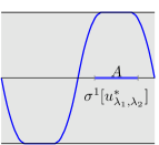
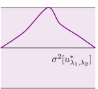
To prove the first item, , we use some (see Figure 2) satisfying
(47) (48) and
(49) With such a function it follows from (45) that
which shows that since .

Figure 2: The figure shows the construction of satisfying (48) and (49). -
b)
To prove the continuity of we use a function which satisfies:
(50a) (50b) (50c) (50d) Such a function is represented in Figure 3.
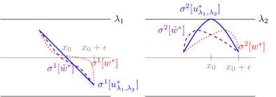
Figure 3: satisfying (50). With such a function it follows from (45), (46), and integration by parts, that
(51) Choosing such that , but otherwise satisfying the same properties as , that are (50a) and (50b), then we obtain
(52) Combining (52) and (51) finally shows
such that we conclude that , which shows that is continuous at .
Item (3): Assume that is as in (44). In the case where
we select some such that
| (53) |
| (54) |
and
| (55) |
Defining
(45) can be rewritten as
Now replacing conditions (53),(54), by
and again using (45) we also obtain . Thus .
(jumping down when ). Using the same arguments as in previous items, we can also proof that .
Lemma 5.12.
Proof 5.13.
Recall that if is different from , then is a polynomial (piecewise). Set .
- 1.
- 2.
-
3.
The proof is analog to (1),(2).
6 Example 1
In the following we calculate the specific minimizers of and -minimization for the test data,
| (56) | ||||
In this case we have
and
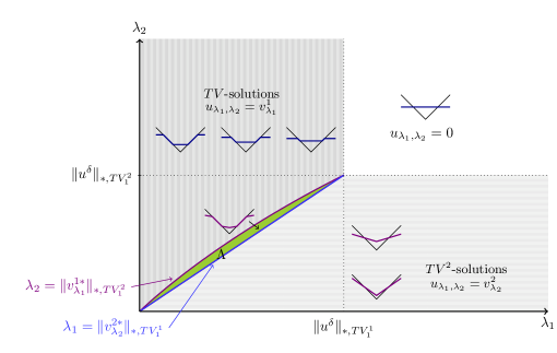
6.1 TV-minimizer
Using the same methods as in [11], we find that for given data (56), the minimizer of the TV-functional is given by
(see Figure 5 (right)).
The function and its dual satisfy the following properties:
-
1.
,
-
2.
, and
-
3.
Hence, from Lemma 5.5 it follows that, as long as
| (57) |
the -minimizer is also the -minimizer and
6.2 -minimizers
6.3 -minimizer
Firstly, we calculate the set (cf. Definition 5.7) for which the -minimizer is different from the -minimizers, respectively. For this particular data this means that for
the minimizer of the -functional equals a minimizer of a -functional , for some .
Let now , which is the only case for which we can expect that the -minimizer is different to -minimizers.
We introduce the two-parametric set of functions , consisting of all functions of the form,
| (59) |
where and . Note that
-
•
is continuous,
-
•
and ,
-
•
for ,
-
•
for .
![[Uncaptioned image]](/html/1309.7152/assets/x10.png)
Assuming that minimizes , Lemma 5.12 provides necessary criteria for optimality of the parameters and , which are derived in the following. Then, in Theorem 6.2 below, we prove that in fact minimizes .
Assuming that is a minimizer of it follows from Lemma 5.12 that:
- •
- •
Using a Computer Algebra system, we solve (60)-(61) and obtain
| (62) |
Remark 6.1.
We want to see what happens for the special case when , that is we consider the two sets of parameters:
Theorem 6.2.
For and , satisfying (62), .
In order to proof the theorem in a compact way, we need the following remark:
Remark 6.3.
In the next two items, we only rewrite as a linear combination of minimizers of , where we have to replace by a different parameter depending on .
-
•
For given set
(63) Comparing the coefficients of the piecewise terms of , we see that for we can write
(64) - •
Proof 6.4.
Using the triangle-inequality and the estimate , we obtain
| (65) | ||||
Due to the definition of and the choice of the parameters , we have that , such that
| (66) |
In order to simplify the left side, we calculate
and
In total we obtain
Comparing with (65) and (66) we have
which together with Lemma 5.12 implies that is a minimizer of .

7 Example 2
Consider now as second test-data
| (67) |
where is the indicator function of the interval . Then
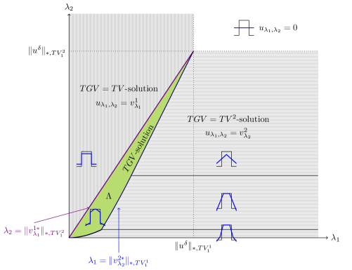
First we calculate minimizers of , as defined in (5), in order to obtain the sets , where, according to Lemma 5.5, the -minimizers are equal to some -minimizers.
7.1 -minimizers
7.2 -minimizers
-
1.
For is bending four times and in a region near . , where is a rational of polynomials of higher order in , not written explicitly here.
-
2.
For is bending at , and in a region near . Moreover .
-
3.
For is bending once and . Additionally we can calculate .
The expressions are used to calculate the set , the set of parameters, where the -minimizer might be different to the or -minimizer.

We write the solutions in the form
| (69) |
keeping in mind that can be 0 (third case), or can be larger then one (third and second case). is bending at , such that is extremal at (hence ). Thus, the coefficients are determined by the following equations:
| cases 1,2,3 | ||||
7.3 -minimizers
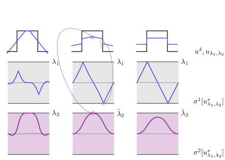
We consider the same approach as for the previous example. Hence, first we calculate the set as in Definition 5.7, which is illustrated as the green (solid) set in Figure 8. We have:
Next we set up a general Ansatzfunction of piecewise affine functions, that is bending, once, twice or four times and jumping at . Setting , we find the coefficients (of the piecewise affine functions) by solving a number of non-linear equations coming from the conditions - whenever the Ansatzfunction jumps and , whenever the Ansatzfunction bends. We omit the explicit formulas and further calculations.
Then for given, we found that the minimizers of can be written in a compact form:
Theorem 7.1.
Proof 7.2.
Lemma 4.2 states that is a
minimizer if
(see
(19)) and .
Using (70) we can estimate by
Since , we have
Note that from the choice of the parameters we have
and also
such that and
| (71) |
Moreover, we can write
Since , and we obtain
Now by the choice of the parameter we have
and
such that the equation above simplifies to
Next it remains to calculate . Since
we have
where we used , the optimality condition for -minimizers as in (18). Hence in total, using the connections between and , we obtain
A Comparison with (71) shows that , hence according to Lemma 4.2 minimizes .
8 Example III
Finally we consider but only sketch the different minimizers of and in order to show that in general, minimizers of cannot be written as a sum of - minimizers. We have .
8.1 -minimizers.
Since is continuous, also the -minimizer is continuous. From the characterization of minimizers we know that is either equal to in an interval or constant in the other intervals. In Figure 9 (left), we ilustrate for different values of .
8.2 -minimizers.
In this case, we have to consider two different types of minimizers.
-
•
large: (that is ), is piecewise constant and bending at . Such solutions are constructed by considering the Ansatzfunctions . The parameter is determined such that (the Ansatzfunction is bending at , hence the of the dual minimizer has be extremal, hence equal to ). This Ansatzfunction works until for some , we have .
-
•
Then for , we use a different Ansatzfunction that satisfies: for and some and is affine linear in and continuous at . The coefficients are determined such that and .
We illustrated both types of solutions in Figure 9 (right).
8.3 -minimizers.
For as in Definition 5.7, we set up an Ansatzfunction that satisfies the following:
-
•
is continuous,
-
•
,
-
•
for and ,
-
•
either is bending at , or for with ,
-
•
is piecewise affine linear else.
We illustrate minimizers for different choices of in Figure 9.
Acknowledgments
This work has been supported by the Austrian Science Fund (FWF) within the national research networks Photoacoustic Imaging in Biology and Medicine (project S10505) and Geometry & Simulation (project S11704). C. P. acknowledges support by the Austrian Science Fund (FWF) within the Schrödinger program (project J-297).
References
- [1] G. Aubert and J.-F. Aujol. Modeling very oscillating signals. Application to image processing. Appl. Math. Optim., 51: 163–182, 2005.
- [2] H. H. Bauschke and P. L. Combettes. Convex analysis and monotone operator theory in Hilbert spaces. CMS Books in Mathematics/Ouvrages de Mathématiques de la SMC. Springer, New York, 2011.
- [3] M. Benning, C. Brune, M. Burger, and J. Müller. Higher-order TV methods–enhancement via Bregman iteration. J. Sci. Comput., 54:269–310, 2013.
- [4] K. Bredies, K. Kunisch, and T. Pock. Total generalized variation. SIAM J. Imaging Sciences, 3(3):492–526, 2010.
- [5] T. F. Chan and S. Esedoḡlu. Aspects of total variation regularized function approximation. SIAM J. Appl. Math., 65(5):1817–1837, 2005.
- [6] P. L. Davies and A. Kovac. Local extremes, runs, strings and multiresolution. Ann. Statist., 29(1):1–65, 2001.
- [7] I. Ekeland and R. Temam. Convex Analysis and Variational Problems. North-Holland, Amsterdam, 1976.
- [8] E. Mammen and S. van de Geer. Locally adaptive regression splines. Ann. Statist., 25(1):387–413, 1997.
- [9] Y. Meyer. Oscillating patterns in image processing and nonlinear evolution equations, volume 22 of University Lecture Series. American Mathematical Society, Providence, RI, 2001. The fifteenth Dean Jacqueline B. Lewis memorial lectures.
- [10] C. Pöschl. Tikhonov Regularization with General Residual Term. PhD thesis, University of Innsbruck, Austria, Innsbruck, October 2008.
- [11] C. Pöschl and O. Scherzer. Characterization of minimizers of convex regularization functionals. In Frames and operator theory in analysis and signal processing, volume 451 of Contemp. Math., pages 219–248. Amer. Math. Soc., Providence, RI, 2008.
- [12] L. I. Rudin, S. Osher, and E. Fatemi. Nonlinear total variation based noise removal algorithms. Phys. D, 60(1–4):259–268, 1992.
- [13] O. Scherzer, M. Grasmair, H. Grossauer, M. Haltmeier, and F. Lenzen. Variational methods in imaging, volume 167 of Applied Mathematical Sciences. Springer, New York, 2009.
- [14] G. Steidl. A note on the dual treatment of higher-order regularization functionals. Computing, 76(1–2):135–148, 2006.
