Fully cosmological virtual massive galaxies at $z=0$: kinematical, morphological, and stellar population characterisation

Abstract

We present the results of a numerical adaptive mesh refinement hydrodynamical and N-body simulation in a $\Lambda CDM$ cosmology. We focus on the analysis of the main properties of massive galaxies ($M_{*}>10^{11}\,M_{\odot}$) at $z=0$. For all the massive virtual galaxies we carry out a careful study of their one dimensional density, luminosity, velocity dispersion, and stellar population profiles. In order to best compare with observational data, the method to estimate the velocity dispersion is calibrated by using an approach similar to that performed in the observations, based on the stellar populations of the simulated galaxies. With these ingredients, we discuss the different properties of massive galaxies in our sample according to their morphological types, accretion histories and dynamical properties. We find that the galaxy merging history is the leading actor in shaping the massive galaxies that we see nowadays. Indeed, galaxies having experienced a turbulent life are the most massive in the sample and show the steepest metallicity gradients. Beside the importance of merging, only a small fraction of the final stellar mass has been formed ex-situ (10-50%), while the majority of the stars formed within the galaxy. These accreted stars are significantly older and less metallic than the stars formed in-situ and tend to occupy the most external regions of the galaxies.

1 Introduction

Understanding the formation and evolution of massive galaxies (i.e. galaxies with stellar mass $M_{*}>10^{11}M_{\odot}$) represents one of the major challenge in the current hierarchical model of galaxy formation. In the nearby Universe, the majority of massive galaxies have the morphology of early-type galaxies, ETG, (Baldry et al., 2004; Renzini, 2006). The bulk of their stars is old and metal-rich (Jørgensen, 1999; Trager et al., 2000; Gallazzi et al., 2005), pushing them on the red sequence in the colour-magnitude relation. Though, several observational evidences also revealed that a small amount of recent star formation is a common feature in massive galaxies (Trager et al., 2000; Bressan et al., 2006; Kaviraj et al., 2007; Sarzi et al., 2008; Tojeiro et al., 2011).

From the dynamical point of view, massive ETGs show the same dichotomy as the general galaxy population. Integral-field kinematics of the SAURON sample (de Zeeuw et al., 2002), has allowed to distinguish two families of ETGs: the slow rotators (SR), having little or no rotation, showing misalignments between the photometric and the kinematic axes, and containing kinematically decoupled cores, and the fast rotators (FR), showing a disk-like rotation (Cappellari et al., 2007; Emsellem et al., 2007; Emsellem et al., 2011). The fast rotators are the most populated family, constituting the $\sim 70\%$ of the ETGs brighter than $M_{K}\sim-24$. Dissipative processes, like gas-rich mergers or gas accretion, are often invoked to explain the formation of fast rotators (Bender, Burstein, & Faber, 1992; Bournaud, Jog, & Combes, 2005; Bois et al., 2012). Dissipationless mergers are instead generally assumed as the most likely mechanism to produce slow rotators (Naab & Burkert, 2003; Cox et al., 2006). The number of major mergers during a galaxy life can also play a role in differentiating among fast and slow rotators (Khochfar et al., 2011).

In conjunction with their old stellar populations, even the assembly process in massive galaxies appears to take place at moderately high redshift, as indicated by the little evolution of the high-mass end of the stellar mass function (Fontana et al., 2006; Pérez-González et al., 2008; Marchesini et al., 2009). The existence of a population of massive, old, and passively evolving galaxies, observed up to $z\sim 2$ (Cimatti et al., 2004; Glazebrook et al., 2004; Cimatti et al., 2008; Whitaker et al., 2013), has opened the question on how to form such galaxies in a $\Lambda$CDM cosmology, where the structure growth is expected to be hierarchical. In this context, the major merger scenario certainly plays a significant role in shaping the present-day massive galaxies. Binary mergers of gas-rich disks has been shown to be a viable mechanism for the formation of spheroidal galaxies (Barnes & Hernquist, 1992; Hernquist, 1992; Cox et al., 2006; Naab, Jesseit, & Burkert, 2006). Although major mergers certainly occur and can explain the existence of massive compact galaxies at high redshift (Ricciardelli et al., 2010; Bournaud et al., 2011), they are too rare and other mechanisms should be active to explain the subsequent evolution. Minor mergers, being much more common (Khochfar & Silk, 2009), are likely to provide this mechanism. They represent also the natural way to explain the strong size evolution of ETGs observed between z=2 and the present time (Daddi et al., 2005; Trujillo et al., 2007; Cimatti et al., 2008; Cassata et al., 2011; Damjanov et al., 2011), while, at the same time, lead to a mild decrease in the velocity dispersion, as observed (Cenarro & Trujillo, 2009; Naab et al., 2009).

The picture emerging from cosmological simulations of massive galaxies (Naab et al., 2009; Oser et al., 2010; Lackner et al., 2012) naturally embeds the minor merger scenario as a fundamental ingredient in a two-phase formation process. In a first phase, galaxies assemble their mass mainly through dissipative processes and star formation takes place in-situ. This in-situ star formation can be induced by cold flow accretion (Kereš et al., 2005; Ocvirk, Pichon, & Teyssier, 2008; Kereš et al., 2009; Dekel et al., 2009) or by gas-rich mergers (Mihos & Hernquist, 1996; Cox et al., 2008). In a second phase, the mass assembly occurs mainly by accretion of satellites. In this phase, mergers occur with typical mass ratio of 1:5. Simulations based on different codes agree in that the ex-situ component is made by older and less metallic stars than the in-situ population (Lackner et al., 2012; Johansson, Naab, & Ostriker, 2012). Hydrodynamical simulations of disc galaxies also find important differences between the in-situ and the accreted components (Zolotov et al., 2009; Font et al., 2011). However, the details on the two-phase galaxy formation are still strongly model dependent and the mass fraction of accreted stars can vary by more than 50% among different models (see for instance Lackner et al. 2012). Differences in the numerical techniques as well as in the sub-grid physics can lead to such important discrepancies (Dubois et al., 2013).

The purpose of this paper is to characterize a sample of simulated massive galaxies from an adaptive mesh refinement (AMR) simulation. We study their zero-redshift properties, in terms of morphology, kinematics and stellar population content and link them to the galaxy merging history. Following the framework of the two-phase galaxy formation we separate the stars formed in-situ from those accreted and study their properties. We couple the outcome of the simulation with stellar population synthesis models in order to present our results in a form as closer as possible to observations, rather than using the raw data from the simulations. The structure of the paper is as follows. In Section 2 and 3 we describe the details of the simulations and of the tools used in the post-processing analysis. In Sections 4 we present one-dimensional profiles of the relevant quantities. In Section 4.2 we describe the properties of the stellar populations formed in-situ and ex-situ. Finally, we draw our conclusions in Section 5. In the appendix we discuss our method to measure the galaxy velocity dispersion.

2 Simulating the Virtual galaxies

2.1 Numerical simulation

The simulation described in this paper was performed with the cosmological code MASCLET (Quilis, 2004). This code couples an Eulerian approach based on high-resolution shock capturing techniques for describing the gaseous component, with a multigrid particle mesh N-body scheme for evolving the collisionless component (dark matter). Gas and dark matter are coupled by the gravity solver. Both schemes benefit of using an adaptive mesh refinement (AMR) strategy, which permits to gain spatial and temporal resolution.

The numerical simulation was run assuming a spatially flat $\Lambda CDM$ cosmology, with the following cosmological parameters: matter density parameter, $\Omega_{m}=0.25$; cosmological constant, $\Omega_{\Lambda}=\Lambda/{3H_{o}^{2}}=0.75$; baryon density parameter, $\Omega_{b}=0.045$; reduced Hubble constant, $h=H_{o}/100km\,s^{-1}\,Mpc^{-1}=0.73$; power spectrum index, $n_{s}=1$; and power spectrum normalisation, $\sigma_{8}=0.8$.

The initial conditions were set up at $z=50$, using a CDM transfer function from Eisenstein & Hu (1998), for a cube of comoving side length $44\,Mpc$. The computational domain was discretised with $128^{3}$ cubical cells.

Two levels of refinement (level $l=1,2$) for the AMR scheme were set up from the initial conditions by selecting regions satisfying certain refining criteria, when evolved – until present time – using the Zeldovich approximation. The dark matter component in the initial refined regions were sampled with dark matter particles eight and sixty four times, respectively, lighter than those used in regions covered only by the coarse grid (level $l=0$). During the evolution, regions on the different grids are refined based on the local baryonic and dark matter densities. The ratio between the cell sizes for a given level ($l+1$) and its parent level ($l$) is, in our AMR implementation, $\Delta x_{l+1}/\Delta x_{l}=1/2$. This is a compromise value between the gain in resolution and possible numerical instabilities.

The simulation presented in this paper uses a maximum of seven levels ($l=7$) of refinement, which gives a peak physical spatial resolution of $\sim 2.7\,kpc$ at $z=0$. For the dark matter we consider three particles species, which correspond to the particles on the coarse grid and the particles within the two first level of refinement at the initial conditions. The best mass resolution is $\sim 2\times 10^{7}\,M_{\odot}$. This is equivalent to use $512^{3}$ particles in the whole box.

Our simulation includes cooling and heating processes which take into account inverse Compton and free-free cooling, UV heating (Haart & Madau, 1996), and atomic and molecular cooling for a primordial gas. In order to compute the abundances of each species, we assume that the gas is optically thin and in ionization equilibrium, but not in thermal equilibrium (Katz, Weinberg & Hernquist, 1996; Theuns et al., 1998). The tabulated cooling rates were taken from Sutherland & Dopita (1993) and they depend on the local metallicity. The cooling curve was truncated below temperatures of $10^{4}\,K$. The cooling and heating were included in the energy equation (see Eq.(3) in Quilis (2004)) as extra source terms.

2.2 Star formation and chemical enrichment

The star formation is introduced in the MASCLET code following the ideas of Yepes et al. (1997) and Springel & Hernquist (2003). In our particular implementation, we assume that cold gas in a cell is transformed into star particles on a characteristic time scale $t_{*}$ according to $\dot{\rho_{*}}=-\dot{\rho}=(1-\beta)\,{\rho}/{t_{*}(\rho)}$ where $\rho$ and $\rho_{*}$ are the gas and star densities, respectively. The parameter $\beta$ stands for the mass fraction of massive stars ($>8\,M_{\odot}$) that explode as supernovae, and therefore return to the gas component in the cells. We adopt $\beta=0.1$, a value compatible with a Salpeter IMF. For the characteristic star formation time, we make the common assumption $t_{*}(\rho)=t^{*}_{o}(\rho/\rho_{{}_{th}})^{-1/2}$, equivalent to $\dot{\rho}_{*}\sim\rho^{1.5}/t^{*}_{o}$ (Kennicutt, 1998). In this way, we introduce a dependence on the local dynamical time of the gas and two parameters, the density threshold for star formation ($\rho_{{}_{th}}$) and the corresponding characteristic time scale ($t^{*}_{0}$). In our simulation, we take $t^{*}_{0}=2\,Gyr$ and $\rho_{{}_{th}}=10^{-25}\,g\,cm^{-3}$. From the energetic point of view, we consider that each supernova dumps in the original cell $10^{51}\,erg$ of thermal energy. In a similar way, we assume that every time that a star forms, it returns to the environment a fraction of metals depending on its mass, $y=\frac{m_{{}_{M}}}{m_{*}}$, where $y$, $m_{{}_{M}}$, and $m_{*}$ are the yield, the mass of metals, and the star mass, respectively. This metal density $(\rho_{{}_{M}})$ allows us to define a metallicity, $Z=\frac{\rho_{{}_{M}}}{\rho}$ which can be used to compute cooling rates for variable metallicities. The metallicity is advected through the computational box using a continuity equation similar to the continuity equation of the gas component. Our stellar formation approach does not take into account the feedback from stellar winds (AGB stars) nor the type Ia supernovae.

In the practical implementation, we assume that star formation occurs once every global time step, $\Delta t_{l=0}$ and, only in the cells at the highest levels of refinement ($l=6,7$). Those cells at these levels of refinement, where the gas temperature drops below $T<2\times 10^{4}\,K$, and the gas density is $\rho>\rho_{{}_{th}}=10^{-25}\,g\,cm^{-3}$, are suitable to form stars. In these cells, collisionless star particles with mass $m_{*}=\dot{\rho}_{*}\Delta t_{l=0}\Delta x_{l}^{3}$ are formed. In order to avoid sudden changes in the local gas density, an extra condition restricts the mass of the star particles to be $m_{*}={\rm min}(m_{*},\frac{2}{3}m_{gas})$, where $m_{gas}$ is the total gas mass in the considered cell. The energy associated to the stellar feedback from supernovae is dumped within the same cell where the stellar particle is created. The adopted value for the yield is $y=0.02$.

2.3 Stellar populations

To convert physical quantities in observables, we employ the MIUSCAT stellar population models (Vazdekis et al., 2012; Ricciardelli et al., 2012), a recently extended version of the MILES (Vazdekis et al., 2010) and CaT models (Vazdekis et al., 2003). The MIUSCAT models are a library of single stellar population spectral energy distribution (SED), covering the spectral range $3500-9500$ Å at moderately high resolution (FWHM $2.5$ Å). The SEDs have been built by combining three empirical stellar libraries: the MILES library (Sánchez-Blázquez et al., 2006) covering the range $\lambda\lambda\,3525-7500$ Å, the CaT library (Cenarro et al., 2001) in the range $\lambda\lambda 8350-9020$ Å and the Indo-U.S library (Valdes et al., 2004), used to fill-in the gap between the MILES and CaT libraries and to extend blueward and redward the spectral coverage of the SEDs.

Each stellar particle in the simulation is treated as a simple stellar population (SSP), formed at a given time with a specific mass, metallicity and a Salpeter IMF. Hence, we can assign a spectrum to each particle by choosing the MIUSCAT model having age and metallicity closest to those of the particle. Finally, to derive fluxes and magnitudes we make use of the SDSS passbands and the AB system.

3 Finding and shaping the virtual galaxies

3.1 The halo finding process

The outcome of our simulation is a complete description of the three components included in the simulation, namely, gas, dark matter and stars. In order to analyse and characterise the properties of the galaxies at the different outputs, we identify the galaxies by means of an adaptive friends of friends algorithm applied only to the star particles. In the practical implementation of our finder, we linked star particles using an iterative process starting from a large linking length of $\sim 100\,Kpc$ and reducing it until a limit length of $\sim 3\,Kpc$. Once all the particles belonging to a given halo are identified by the iterative linking process, they undergone an extra process to check whether they are gravitationally bound to the systems. Those unbounded particles are drop off the list of members of such galaxy. We experimented intensively with the different choices of linking lengths, being the previous one the most stable. Finally, we build the merger tree of each halo by looking at its progenitors at the previous snapshots of the simulation. We consider 31 snapshots between z=4 and z=0, with a typical time interval of 0.5 Gyr. The main progenitor is defined as that halo that contributes the most to the stellar mass of the final halo. When more than one progenitor are present, we consider that a merger has taken place when the mass ratio between the main progenitor and the satellite is higher than 0.025. Therefore, the accretion of very small haloes is not considered as a merger event. We do not carry out any special treatment to identify satellites, as we are only interested in tracking the smaller galaxies that eventually would merger with the main progenitor of the final galaxy.

The result of the halo finding process is a complete sample of all the galaxy-like objects in our simulation at the different redshifts. Every galaxy is perfectly defined and all its properties determined, therefore, the generated catalogue can be used to explore the properties of the galaxies and to compare with the observational plane.

The analysis of the virtual Universe generated by our simulation by means of the previously described halo finder, produces a sample of galaxies spreading over a huge range of masses and sizes. In the present work, we focus our analysis on the more massive galaxies in the sample, those with zero-redshift stellar masses $M_{*}>10^{11}\,M_{\odot}$. The total number of galaxies in our sample satisfying such mass condition is 33. Galaxies in the process of merging are excluded from the analysis, as their dynamical and morphological state are far from being relaxed, hence difficult to characterize. We have therefore restricted the sample to galaxies that have not undergone very recent merger events and that are located in the higher resolution grid. This leaves us with a sample of 21 galaxies more massive than $10^{11}M_{\odot}$.

3.2 Baryon conversion efficiency

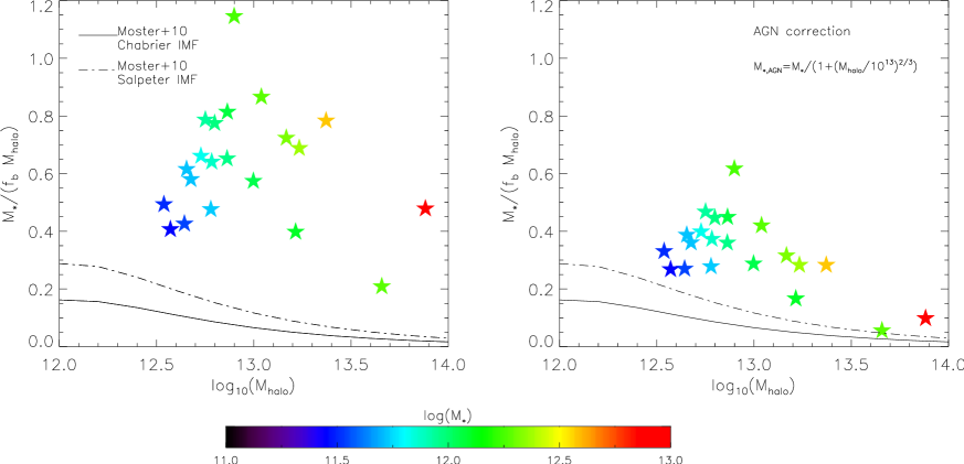
Figure 1: Stellar to halo mass ratio as a function of halo mass for the 21 massive galaxies in our sample. Points are coloured according to the palette representing the galaxy stellar mass, with the reddest points being the most massive galaxies. We also show the results of Moster et al. (2010) from abundance matching tecniques for a Chabrier IMF (solid line) and Salpeter IMF (dashed line). In the left-hand panel we use the original stellar masses from the friend of friends halo finder, while in the right-hand panel we show the effect on the stellar masses that we would expect from the inclusion of AGN feedback. See text for further details.

Since in our simulation we do not include AGN feedback, we expect our stellar masses to be significantly biased towards higher masses. To quantify the efficiency of conversion of baryons into stars, in Figure 1 we show the baryonic conversion efficiency: $f_{conv}=M_{*}/(f_{b}M_{halo})$, where $f_{b}=\Omega_{b}/\Omega_{m}$ is the cosmic baryon fraction, as a function of halo mass. Halo masses have been determined by means of the code ASOHF (Adaptive Spherical Overdensity Halo Finder, Planelles & Quilis 2010), applied to the dark matter particles. As a comparison, we also show the observational results from abundance matching tecniques from Moster et al. (2010). The original stellar masses of Moster et al. (2010) have been calculated assuming a Chabrier IMF (solid line in Figure 1). Hence, to compare to our Salpeter-based stellar masses we translate them according to Cimatti et al. (2008): $log(M_{Salpeter})=log(M_{Chabrier})+0.25dex$ (dashed line).

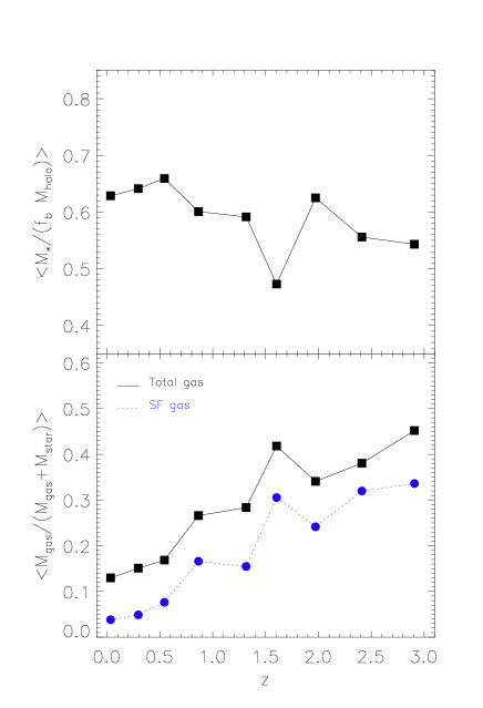
Figure 2: Redshift evolution of the average baryonic conversion efficiency (upper panel) and of the gas fraction (lower panel). In the lower panel, the black line indicates the gas fraction when the total gas mass is considered and the blue line stays for the gas fraction when only the star forming gas is taken into account.

Our galaxies appear overly massive for the halo in which they live. The mean conversion efficiency for the whole sample is $f_{conv}=0.63$, whereas the observations predict, for the same range of halo masses, $f_{conv}\sim 0.15$. However, since in the simulation we do not take into account AGN feedback, we expect massive galaxies to be extremely efficient in the formation of stars. As suggested by Cen (2011), the effect of AGN feedback is to alter the stellar masses by a factor: $f_{AGN}=1/({1+(M_{halo}/10^{13})^{2/3}})$. Hence, in the right-hand panel of Figure 1 we show the baryonic conversion efficiency using the stellar masses corrected by this factor. The mean conversion efficiency significantly reduces to $f_{conv}=0.33$, though a discrepancy of a factor 2-3 persists. As shown in Figure 2, this over-efficient star formation occurs at all epoch at a quite constant rate. Thus, the stellar mass assembly of the massive galaxies appears regulated only by the dark matter merger rate. In the lower panel of Figure 2, we show the redshift evolution of the gas fraction for the total gas mass, $M_{gas}/(M_{gas}+M_{stars})$, and the star forming gas, $M_{SFgas}/(M_{SFgas}+M_{stars})$. The mass of the star forming gas is given by summing up the mass of the halo cells with $T<2\times 10^{4}\,K$ and $\rho>\rho_{{}_{th}}=10^{-25}\,g\,cm^{-3}$ (see Section 2.2). The gas fraction shows a strong evolution with cosmic time, indicating that the progenitors of the massive present-day galaxies at high redshift are gas-dominated systems. At low redshift, massive galaxies contain a small but not negligible amount of gas, with mean values of the gas fraction of 0.13 and 0.04, for the total gas and the star forming gas, respectively.

It is already known that hydrodynamical simulations lacking AGN feedback tend to produce too many stars, leading to too massive galaxies. The problem is common to both smoothed particle hydrodynamics (SPH) and grid codes, but it appears more pronounced in the latter. For instance, in Oser et al. (2010) (SPH code GADGET-2), the overproduction of baryons is less serious, with a conversion efficiency of the order of $f_{conv}\sim 0.2$ for the same range of halo masses probed here. On the other hand, simulations using AMR codes tend to produce higher conversion efficiencies. Indeed, Lackner et al. (2012) and Dubois et al. (2013) (in the simulation without AGN feedback) found a conversion efficiency very similar to ours for a similar halo mass range. In the Dubois et al. (2013) simulation with AGN feedback, the baryonic conversion efficiency reduces down to a value of 0.1, leading to stellar masses in a better agreement with the expectations from abundance matching techniques, although in the most-massive haloes they remain too massive. It is important to notice that if the AGN feedback were as strong as suggested by Dubois et al. (2013), the corrections applied to our stellar masses in Figure 1 would be then underestimated. Indeed, the values of the star forming gas fraction shown in Figure 2 are in good agreement with those found by Dubois et al. (2013) for the no AGN case. As shown by those authors, the inclusion of a radio mode feedback is particularly effective in reducing the amount of star forming gas at low redshift, thus suppressing the late star formation and bringing down the discrepancy with observations.

Several reasons can contribute to explain the differences found among different codes. Spatial and mass resolution can in principle affect the results on the star formation efficiency, with low-resolution simulations expected to give higher late star formation. We have a mass resolution comparable with that of Oser et al. (2010), but a coarser spatial resolution, although the smoothing length in SPH cannot be directly compared to the cell size of AMR codes. We expect that an improved resolution can help in reducing the problem, but we should note that AMR simulations using higher spatial resolution than that used here (Lackner et al., 2012; Dubois et al., 2013), produce the same amount of over-production of stars. Hence, we do not expect that improved resolution would be the only solution. The star formation efficiency can also affect the final results, because higher efficiencies produce higher star formation at high redshift and a lower level of late star formation. However, Dubois et al. (2013) have shown that an increased star formation efficiency does not lead to significant changes in the final stellar mass. We also note that the star formation efficiency used in this work is similar to that used in Oser et al. (2010).

Hence, we are prone to think that in the absence of AGN feedback, the amount of gas converted into stars is primarily regulated by the cooling efficiency. Comparisons between SPH and grid codes (sharing same physics and same initial conditions) have led to the conclusion that SPH codes produce less efficient cooling rate. This naturally translates in lower levels of star formation rate and less massive galaxies (Kereš et al., 2012; Scannapieco et al., 2012). The reason for that would be in the different treatment of shocks and gas instabilities among the two numerical techniques. As demonstrated by Agertz et al. (2007), gas instabilities are not correctly solved in SPH codes. The different treatment of hydrodynamical instabilities in the two numerical techniques can lead to importance differences in the dissipation heating. Vogelsberger et al. (2012) have shown that SPH codes produce a significant heating in the outer part of the haloes, where the cooling radius is expected to lie. This produces an overall higher temperature and a weaker cooling efficiency that can explain the lower level of star formation in these simulations (see also Kereš et al. 2012). However, this dissipation in SPH is likely to be of spurious nature and ultimately caused by errors in the estimation of pressure gradients. This different behavior of SPH and grid techniques could be than a potential source of discrepancy among the Oser et al. (2010) findings and our results.

3.3 Two dimensional maps

A proper characterization of the morphological structure of the simulated galaxies requires to treat them as close as possible to real objects. To this aim, the 3D structure of a galaxy has been converted in a 2D map by projecting its volume of star particles onto a plane. To overcome the resolution limit we choose a pixel size in the 2D image equal to the spatial resolution of the MASCLET level where the galaxy is located. Since we have selected only galaxies in the highest level of refinement ($l=7$), the pixel size of the 2D map is 2.7 kpc for all the galaxies in the sample, that roughly corresponds to $R_{e}/4$ for the smallest galaxies and $R_{e}/8$ for the largest ones. The galaxies have been projected along each one of the coordinate axes of the computational box. In this way we create three different 2D maps for every simulated galaxy. These 2D projections have been used to get the 1D profiles described in the next section.

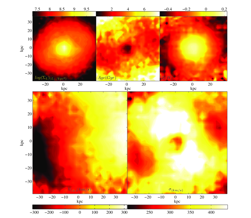
Figure 3: 2D map of one of the most massive galaxies in our sample ($M_{*}\sim 3.3\times 10^{12}\,M_{\odot}$ or $M_{*}=1.5\times 10^{12}\,M_{\odot}$ after AGN correction, $R_{e}=14.2\,Kpc$) . Top panels represent, from left to right: logarithm of the surface density mass, age of the stellar population, and metallicity in solar units. Bottom panels show the line-of-sight velocity (left) and the velocity dispersion (right). According with the three classification criteria described in Sec. 4, this galaxy is just at the transition between the fast and slow rotator types from its dynamics. Its history labels it as a merger galaxy, whereas its morphology indicates that it is an elliptical galaxy.

To create the artificial images, the total flux in every pixel is computed by summing up the flux of each SSP weighted according to its mass. To limit the galaxies to their visible part we only consider pixels whose surface brightness (SB) in the r-band is brighter than 25 mag/arcsec², which corresponds to typical limiting SB in the observations. An example of artificial images for a representative galaxy in the sample is shown in Figure 3. Artificial images have been used to derive the galaxy structural parameters through the two-dimensional fitting code GALFIT (Peng et al., 2002). The light distribution of the simulated galaxies has been modelled with a Sérsic profile (Sérsic, 1968), deriving the Sérsic index $n$, the semi-major effective radius $R_{e}$ and the axial ratio $b/a$. Although in the following we make use of the Sérsic fits derived by means of 1D profiles, the axial ratio assigned to each galaxy is the one derived with GALFIT.

Moreover, the use of two-dimensional grids allows us to measure the velocity dispersion along the line-of-sight (LOS) in a consistent way. Once we have computed the mean velocity of the stellar particles in each pixel, the velocity dispersion of the particles in the cell is estimated through the square deviations of particle velocities from this mean value (see the Appendix). Therefore, the velocity dispersion in the individual pixels does not need any further correction for galaxy rotation.

In Figure 3 we show, as an example, the 2D maps of the relevant quantities analyzed in the present work for one of the most massive galaxies of the sample.

4 Results

We study the sample of massive galaxies and their more relevant features attending to three wide criteria: (i) their dynamical properties, (ii) their evolutionary history, and (iii) their morphologies.

As a first step, we classify the galaxies in our sample according to the dynamics. To do so, we look at a quantity widely used in the literature (e.g. Emsellem et al. (2011)): the ratio of the rotational velocity to the dispersion velocity ($V/\sigma$). This quantity allows us to split the sample into two groups, the slow rotators and the fast rotator objects.

The second criteria that we use to study the galaxies in our sample is their evolutionary history. Thus, according to their evolution, we separate the galaxies in two categories: those galaxies which have suffered at least a merger event, and those other galaxies that have a quiet evolution without any mergers recognized by the halo finder. Thus, the merger sample also includes galaxies having experienced only minor mergers.

Finally, the third criteria used to sort the sample is the morphology. The basic methodology consist in fitting the light profile of each object by the corresponding Sérsic profile and obtain the Sérsic index ($n$).

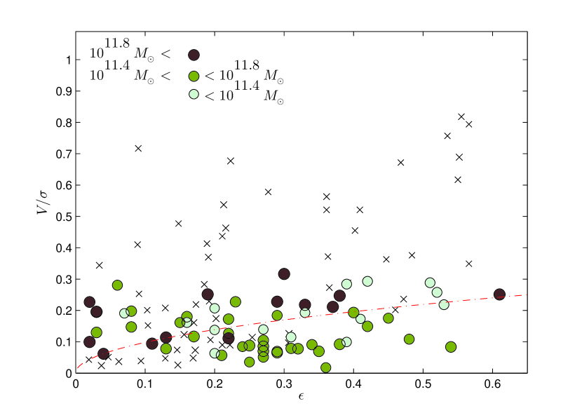
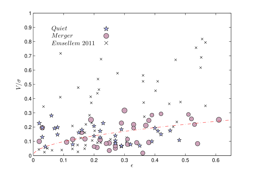
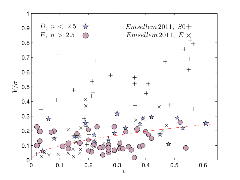
Figure 4: $V/\sigma$ vs ellipticity diagram for our simulated galaxies (color symbols). For the sake of comparison, crosses indicate the position in the diagram of the most massive galaxies in the ATLAS sample of Emsellem et al. (2011), whereas the red dot-dashed line is $V/\sigma=0.3\sqrt{\epsilon}$, used to discriminate slow and fast rotators. In the top panel galaxies are colored according to their stellar mass, and in the middle (bottom) panel they are separated according to the merger history (morphology). In the bottom panel, the observational data points are also separated into early-type galaxies and lenticulars.

In order to make our results more consistent with the observational data, and according with the previous discussion in Sec. 3.2, all the galaxy masses in the sample are corrected following the prescription by Cen (2011). This post-processing of the galaxy masses allows us to modify our results for the stellar masses in a way that tries to mimic the effects of the AGN feedback. We have also to remark that the rest of the galaxy properties that could change due to AGN feedback, like stellar populations and velocity dispersion, are kept unchanged.

4.1 One dimensional profiles

One dimensional (1D) profiles are useful tools to compare the results of the simulations with observational data. To produce 1D profiles as similar as possible to the ones produced by observations, we perform the following procedure.

In each of the three projections we identify the center of the 2D map. This is done in a two steps process. First, the centre is computed as the centre of luminosity or mass, depending on whether we consider mass or light weighted profiles, of all the star particles forming the galaxy. Then, the effective radius ($R_{e}$) is defined as the half light (mass) radius. As for the total luminosity (mass) used to determine the effective radius, we only consider the luminosity (mass) in cells whose SB is brighter than 25 mag/arcsec². A finer determination of the centre of the galaxy is given by computing the centre of luminosity (mass) only with the particles inside the half light or mass radius. Finally, starting from the centre, the radial 1D profile for the considered quantity is obtained by averaging in circular shells whose width is such that contains one per cent of the total mass of the galaxy for mass weighted profiles or one per cent of the total flux in the case of light-weighted profiles. We choose this particular binning in order to be able to reach the external part of the galaxies, while at the same time achieve smooth profiles.

The previously described process allows us to produce 1D profiles of every galaxy in our sample. In particular, we analyse the following quantities: luminosity $\Sigma_{L}$, surface density $\Sigma_{M}$, velocity dispersion $\sigma$, line of sight velocity $V$, age and metallicity $Z$.

Depending on the analysed criteria, galaxies are gathered in different groups. All the 1D profiles of the galaxies in the same group are averaged. The following figures shown in this Section present these 1D median profiles and the $25^{th}/75^{th}$ percentile as shaded regions. We use the luminosity in the r band to light-weight the 1D profiles.

4.1.1 Dynamics

In numerical simulations, the definition of a quantity representing the velocity dispersion ($\sigma$) is somehow vague and can be defined in many different manners. Although, all those definitions can be self-consistent in the simulations, it becomes crucial how $\sigma$ is defined when the virtual galaxies in the simulations are compared with observed ones. In order to get rid of this ambiguity, we have found the best definition of $\sigma$ in the simulations to compare with observations. In Appendix A, we present a detailed explanation of the method used to estimate the velocity dispersion. In brief, we find that a luminosity weighted mean of the square deviations of the particle velocities (eq. 5) shows a close agreement with the velocity dispersion derived from the spectral features.

As a proxy to characterize the rotational structure of our numerical sample of galaxies, we have used the ratio of ordered to random motion in a galaxy ($V/\sigma$), both projected along the line-of-sight (LOS) We have also checked that by separating the dynamical groups by means of the $\lambda$ parameter, as defined in Emsellem et al. (2011), the results of this section do not change substantially.

In Figure 4 we present the anisotropy diagram, relating this parameter to the observed ellipticity ($\epsilon$). The ellipticity is defined as $\epsilon=1-b/a$, where $b/a$ is the galaxy axial ratio, measured by means of GALFIT. Following the approach used in integral-field studies (Cappellari et al., 2007; Emsellem et al., 2011), $V/\sigma$ is defined by:

$$\Big{(}\frac{V}{\sigma}\Big{)}^{2}=\frac{\sum\limits_{i=1}^{N}{L_{i}V_{i}^{2}}}{\sum\limits_{i=1}^{N}{L_{i}\sigma_{i}^{2}}}$$ (1)

where the summation extends over the stellar particles lying within the effective radius, $L_{i}$ is the particle luminosity and $V_{i}$ and $\sigma_{i}$ are the LOS velocity and velocity dispersion associated to the star particle. In the upper panel of Figure 4, our data are shown as circles colored according to their masses. For each galaxy, all the three projections are shown. Overplotted to our data, in Figure 4 we show the position in the diagram of the most massive galaxies (selected to have magnitude in the K-band brighter than $-23.8$ mag) in the ATLAS sample (Emsellem et al., 2011). According to these authors, fast and slow rotators can be well separated in the $V/\sigma$-$\epsilon$ plane using as threshold: $V/\sigma=0.3\sqrt{\epsilon}$, that is shown as a magenta dot-dashed line in Figure 4. Therefore in the following we define slow-rotators (S) the galaxies lying below this line, that constitute the 54% of the total sample and fast-rotators (F) the remaining galaxies (46%).

The simulated galaxies span a wide range of rotational properties, in agreement with the distribution observed for the bright ATLAS galaxies. However, the simulated galaxies do not reach the highest values of $V/\sigma$ displayed by the observed galaxies. Indeed, the fraction of fast rotators in the ATLAS sub-sample is 69%, higher than our value.

Stellar mass does not seem to play a crucial role in discriminating among fast and slow rotators, as the fraction of fast rotators (slow rotators) is similar in the three mass intervals considered. Likewise, by dividing the Emsellem sample in three bins according to their luminosity, we get the same result, i.e. the fraction of F (S) does not change with luminosity.

Although both quiet and merger galaxies can be fast rotators, the highest values of $V/\sigma$ are reached by galaxies having undergone mergers. Moreover, fast rotators are usually classified as late-type galaxies (see bottom panel of Fig. 4), in agreement with the Emsellem sample of fast rotators that show S0 morphology.

Figure 5 presents the main properties of the galaxies in the numerical sample classified according to their values of $V/\sigma$. As all the 1D plots in this Section, lines represent the median of all the profiles of the galaxies in every group and the shaded regions stand for the $25^{th}/75^{th}$ percentile of the distribution. The panels represent: luminosity (top left), surface density (top right), dispersion velocity (middle left), line of sight velocity (middle right), luminosity-weighted age (bottom left) and luminosity-weighted metallicity (bottom right). The blue solid line and the blue shaded region correspond to the fast rotator objects, whereas the red dashed line and the shaded region stand for the slow rotators. In order to average all the profiles corresponding to the galaxies in each group, the radial profile of each galaxy is rescaled to its effective radius, $R_{e}$.

Figure 5: 1D profiles for the galaxies in the sample grouped according to their dynamics: slow rotators (S) with $V/\sigma<0.3\sqrt{\epsilon}$ and fast rotators (F) with $V/\sigma>0.3\sqrt{\epsilon}$. The lines represent the median of all the profiles of the galaxies in every group and the shaded regions stand for the $25^{th}/75^{th}$ percentiles of the distribution. The panels represent: surface brightness (top left), surface density (top right), velocity dispersion (middle left), line of sight velocity (middle right), luminosity-weighted age (bottom left), and luminosity-weighted metallicity (bottom right). The blue solid line and the blue shaded region correspond to the fast rotators (F), whereas the red dashed line and the shaded region stand for the slow rotators (S). In the top left panel the black dashed (solid) lines are the Sérsic fits to the median light profiles of the slow (fast) rotators. To average all the profiles corresponding to the galaxies in each group, the radial profile of each galaxy is rescaled in units of its effective radius, $R_{e}$. The surface density and brightness profiles of each galaxy are normalized to their values at $R_{e}$. All profiles displayed in this figure are light-weighted and they are calculated starting at $0.25R_{e}$.

The fast rotator (slow rotator) galaxies have a median stellar mass of $M_{{}_{F}}\sim 7\times 10^{11}\,M_{\odot}$ ($M_{{}_{S}}\sim 6\times 10^{11}\,M_{\odot}$) and a velocity dispersion at the effective radius of $\sigma_{{}_{F}}\sim 219\,km/s$ ($\sigma_{{}_{S}}\sim 247\,km/s$). These previous stellar masses are the values taking into account the AGN correction. For the sake of completeness, the stellar masses without correction are $M_{{}_{F}}\sim 9\times 10^{11}\,M_{\odot}$ and $M_{{}_{S}}\sim 1\times 10^{12}\,M_{\odot}$. Although the light and mass profiles of the two galaxy groups look like quite similar, there is a tendency for the slow rotators to have higher Sérsic indices ($n_{S}\sim 3.0$) than galaxies with higher rotational support ($n_{F}\sim 1.7$). As expected, there are differences in the line of sight velocity, with the fast rotators presenting higher values of $V$ within the effective radius and therefore higher rotation. The velocity dispersion within the effective radius is very similar in the two groups, but at larger radii the velocity dispersion of the fast rotators decays more rapidly.

The analysis of the stellar populations of the two groups is summarized in the two bottom panels of Figure 5. There are significant age gradients in both groups. The general trend is a positive age gradient, meaning younger ages at the center that translates into steeper age gradients within the effective radius for both groups of galaxies. Our findings of positive age gradients is consistent with the observational result of La Barbera et al. (2012) and Coccato, Gerhard, & Arnaboldi (2010), that have determined radial profiles of early-type galaxies out to large galactocentric distances. In the case of the metallicity, both groups show negative gradients, with the slow rotators having a slightly lower metallicity. Despite the trends found in the age and metallicity profiles, we must warn on the values of the ages, which are too low, and the the metallicities at the center which do not reach solar values as it would be more consistent with observational data.

4.1.2 History

In an hierarchical scenario for the formation of cosmic structures, mergers have a crucial role as they sculpt the main features of the galaxies and galaxy clusters. Therefore, the evolutionary history of galaxies is an important key to understand their actual properties (Mihos & Hernquist, 1994; Cox et al., 2006; Hopkins et al., 2009). Within this paradigm, there must be substantial differences between those objects which have had a relatively quiet life (with no important merger events) and those involved in major merger processes.

Following a similar procedure than in subsection 3.1.1, we group the galaxies in the sample separating those which have undergone mergers (M, 52%) and those that have had a quiet evolution (Q, 48%). We assume that a merger has token place when the mass ratio between the satellite and the main progenitor is larger than 0.025. Among the mergers, only few of them (21%) can be considered a major merger (those events with a mass ratio between the objects involved in the merger larger than $\sim 0.3$). Thus, the majority of merger in the simulation (79%) are classified as minor ones, with an average mass ratio of the galaxies involved around $0.17$. The M (Q) type galaxies have a median stellar mass – including the AGN feedback correction – of $M_{{}_{M}}\sim 8\times 10^{11}\,M_{\odot}$ ($M_{{}_{Q}}\sim 6\times 10^{11}\,M_{\odot}$), a Sérsic index fitted from the median light profile $n_{{}_{M}}\sim 1.7$ ($n_{{}_{Q}}\sim 2.8$), and a velocity dispersion at the effective radius of $\sigma_{{}_{M}}\sim 256\,km/s$ ($\sigma_{{}_{Q}}\sim 223\,km/s$). For the sake of completeness, the uncorrected stellar masses are $M_{{}_{M}}\sim 1.6\times 10^{12}\,M_{\odot}$ and $M_{{}_{Q}}\sim 1.1\times 10^{12}\,M_{\odot}$.

We also characterize the kind of merger occurred by looking at the SFR at the time of merger. A dissipational merger can be defined as that merger triggering a strong starburst. Several studies of star forming galaxies indicate the existence of a main-sequence in the SFR-$M_{*}$ plane where most of the star forming galaxies lie (Daddi et al., 2007; Noeske et al., 2007; Rodighiero et al., 2011; Whitaker et al., 2012). A deviation from this sequence towards high SFR indicates the occurrence of a starburst. Taking into account the redshift dependence of the SFR-$M_{*}$ normalization, we adopt the criterion defined in Whitaker et al. (2012) to establish the presence of the starburst during a merger event:

$$log(SFR)>\alpha(z)(logM_{*}-10.5)+\beta(z)+0.34$$ (2)

where $\alpha(z)=0.70-0.13z$ and $\beta(z)=0.38+1.14z-0.19z^{2}$, $M_{*}$ is the mass of the galaxy after the merger and the value of 0.34 dex represents the $1\sigma$ scatter used to define the outliers. Concerning the SFR, we use the mass of gas converted in stars during the last time-snapshot before the merger is identified. We find that 10 out of 11 merging galaxies have undergone a dissipational merger, while just in one case the merger can be considered dry.

In Figure 6, we present – in a similar way than in Fig. 5 – the median profiles for the studied quantities for the two groups of galaxies: $\Sigma_{L}$, $\Sigma_{M}$, $\sigma$, $V_{{}_{LOS}}$, age, and metallicity.

Figure 6: The same as Figure 5 when galaxies are split according to their merging history. Red lines and shaded regions stand for galaxies having experienced a merger (M), while blue corresponds to galaxies with a quiet life (Q).

According to the expectations, the evolutionary history of galaxies seems to be an important factor determining their features. Although light and density profiles in Fig. 6 are very similar, as it happened in the study based on the dynamics, in all the other analysed quantities the differences are notable. Thus, galaxies which have undergone mergers (M) exhibit larger velocity dispersion at all radii and a strong velocity dispersion profile, which is almost flat within the effective radius and decays abruptly outside. The line of sight velocity is also higher for the M galaxies except at the inner part ($R<0.5R_{e}$), where both types of galaxies show similar values. These low values indicate that the very central parts do not present an important rotation regardless the evolutionary history of the galaxy. At outer radii ($R>R_{e}$), the rotational support of the M galaxies increases significantly. Numerical simulations of mergers (Cox et al. 2006) have indeed shown the relevance of the merger-induced dissipation in the formation of fast rotators. Since the majority of the mergers suffered by our simulated galaxies involves a significant fraction of SFR, our results are consistent with those findings.

The galaxies without mergers (Q) are older at all radii and less metallic out to the external regions.

The younger nature of the merger galaxies is not a surprising result given the fact that the majority of mergers have triggered a starburst rejuvenating the stellar populations. At the same time, the star formation occurring in an already enriched medium can produce metal-rich stars, explaining the metallicity trend. The most remarkable feature in the stellar population profiles is the steepness of the metallicity gradient of the M galaxies. A number of studies have explored the role of dissipationless mergers in the formation of stellar population gradients (Kobayashi, 2004; Di Matteo et al., 2009), finding a flattening of the metallicity gradient in the remnants, mainly due to stellar mixing. However, if the merger is dissipational, as in our galaxies, a rejuvenation of the stellar contents in the central region is expected, establishing a steeper metallicity gradient than that of the progenitor galaxy (see for instance Hopkins et al. 2009).

We have verified that the trends found with the merging history are not just an effect of the different mass of the two groups or the nature of the merger events (major or minor). To do this, we repeat the analysis using two subsamples having similar masses and considering only major mergers or minor mergers in the M class. We find no substantial changes in the trends found in Figs. 6. The only worth mentioning difference is the presence of a steeper metallicity gradients in the major merger subsample, whereas the subsample formed by the galaxies that had experimented minor mergers, exhibits metallicity gradients more similar to those of the Q galaxies. Major mergers are thus the first cause for the steeper metallicity gradients observed in Fig. 6. Therefore, the results on the dynamical profiles, the age and metallicity gradients are robust against the definition of the M/Q classes.

4.1.3 Morphology

To classify galaxies according to their morphology we fit the 1D density profile with a Sérsic model, deriving the Sérsic index, $n$, the half-light radii, and the effective luminosity density. The radial interval taken into account in the fits ranges from $0.25R_{e}$ up to $10R_{e}$. The Sérsic index is a common indicator used to classify the morphology of galaxies (Blanton et al., 2003; Ravindranath et al., 2004). Thus, galaxies with values for $n$ larger (smaller) that 2.5 are classified as elliptical (spirals). By using this classification, Figure 7 presents, as usual in this Section, the average properties of the galaxies in the sample classified according to their Sérsic index, $n$, into elliptical (E, 70%) and disk-like (D, 30%) galaxies. As a general rule, the morphology classification derived by fitting the one-dimensional light profiles well agrees with that determined by means of GALFIT, although galaxies with intermediate Sérsic indices ($n\sim 2.5$) can be in a few cases misclassified.

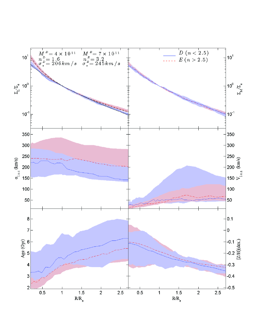
Figure 7: The same as Figure 5 when galaxies are split according to their morphology. Red lines and shaded regions stand for early-type galaxies (E), while blue stands for disk-like galaxies (D).

In Figure 7, we present – in a similar way than in Fig. 5 – the median profiles for the studied quantities for the two groups of galaxies: $\Sigma_{L}$, $\Sigma_{M}$, $\sigma$, $V$, age, and metallicity. The mean stellar mass considering the AGN feedback correction for E (D) galaxies is $M_{{}_{E}}\sim 7\times 10^{11}\,M_{\odot}$ ($M_{{}_{D}}\sim 4\times 10^{11}\,M_{\odot}$). If the AGN correction is not considered, the mean stellar masses are $M_{{}_{E}}\sim 1\times 10^{12}\,M_{\odot}$ and $M_{{}_{D}}\sim 7\times 10^{11}\,M_{\odot}$.

A mean Sérsic index, $n$, for both morphology groups has been derived by fitting the median profiles, obtaining 1.6 and 3.2 for the disc and the elliptical galaxies, respectively. These values allow to clearly differentiate between the two considered morphological types.

As expected, the light and density profiles are more different between the two types of galaxies than in any of the other classification previously used. The dispersion velocity for both D and E galaxies is quite similar at the inner parts and gets larger for elliptical galaxies compared with spiral galaxies as radial distance increases.

There are relevant age gradients in both categories of galaxies, with the internal part substantially younger than the outer parts. The elliptical galaxies are younger than disk galaxies at all radii. Observed ellipticals are instead older than galaxies with a disk-like morphology. The fact that we are not able to reproduce the observed trend can be partly explained with the fact that our galaxies are not able to quench star formation efficiently. This leads to a tail of star formation at low redshift that contributes significantly to rejuvenate the stellar population of both kind of galaxies. We argue that by improving the feedback scheme and the spatial resolution, we would alter the star formation history of these galaxies. Finally, metallicities and metallicity gradients are very similar for both subsamples.

4.2 Star formation history: in-situ vs accreted

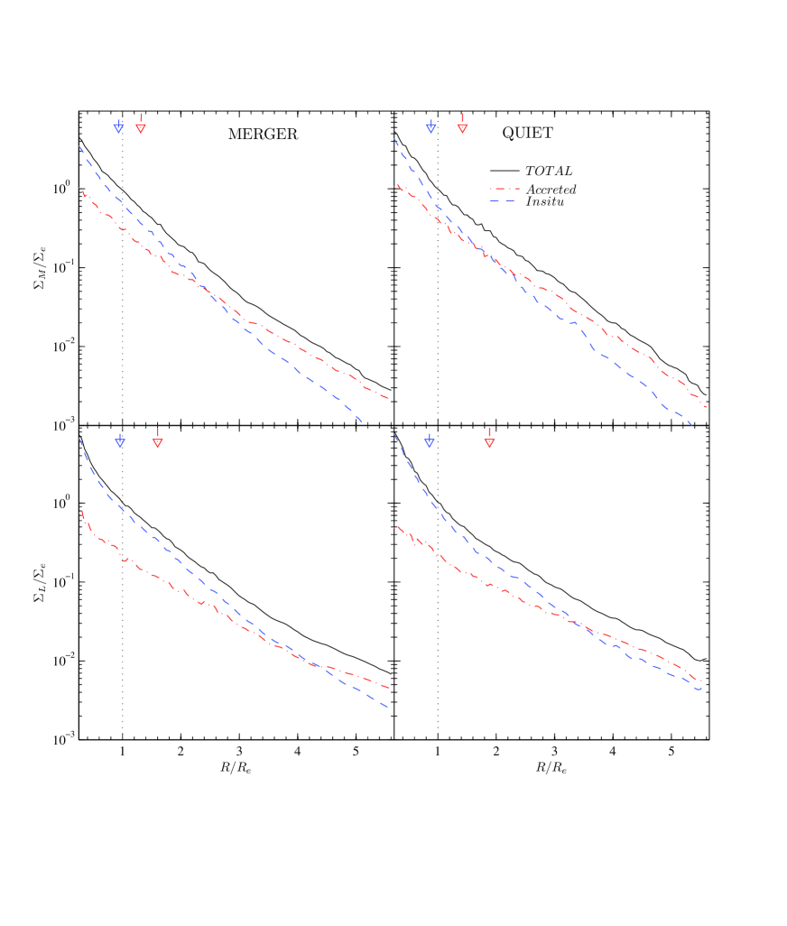
Figure 8: Mass density (upper panels) and luminosity density (lower panels) profiles for the Merger (left panels) and Quiet (right panels) galaxies. The contribution to the total density (black solid) is divided into the in-situ (blue dashed line ) and accreted (red dot-dashed line) components. The arrows indicate the half-mass or effective radii of the in-situ and accreted populations in terms of the galaxy effective radius.

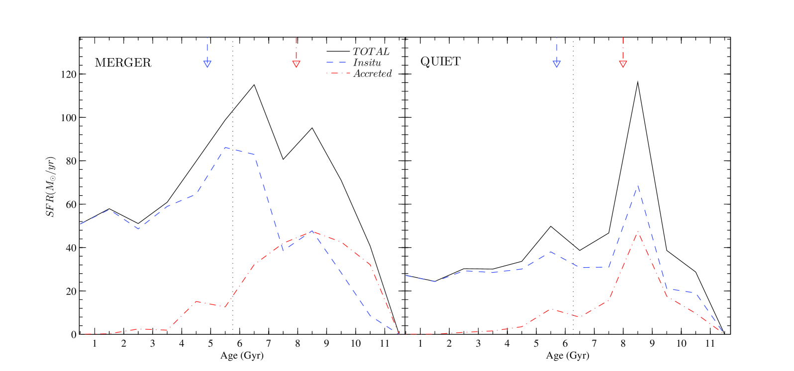
Figure 9: Mean star formation histories of galaxies belonging to the M (left-hand panel) and Q samples (right-hand panel). The black solid line indicates the total SFR, the red dot-dashed line stays for the accreted component and the blue dashed line for the in-situ population. The dotted vertical line represent the mass-weighted mean age of the global population and the arrows indicate the mean ages of the in-situ (blue) and accreted (red) components.

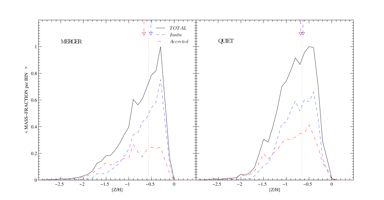
Figure 10: Mean metallicity distribution of galaxies belonging to the M (left-hand panel) and Q samples (right-hand panel), normalised to the maximum mass mass-fraction. Lines are as in Figure 9. The dotted vertical lines and arrows indicate the mass-weighted mean metallicity of the global population and of the two components.

According to recent simulations, galaxy evolution seems to be well described by a two-phase model (Naab et al., 2009; Johansson et al., 2009; Oser et al., 2010; Lackner et al., 2012). The first phase is a period of in-situ star formation and could resemble the monolithically model of galaxy formation (Eggen, Lynden-Bell, & Sandage, 1962; Larson, 1975). The rest of the stars forming the galaxies are accreted via mergers, constituting the second phase. In this Section, we study the differences between these two populations of stars: in-situ and accreted. In particular, we focus on their differences concerning the stellar populations and spatial distribution.

We define as in-situ those stars formed in the main progenitor of the present-day galaxy, whereas the ex-situ (or accreted) component are the stars formed outside the main unit and accreted later, via merger or smooth accretion. To differentiate among in-situ and ex-situ stars, we flag each stellar particle with the halo identifier of the galaxy where it was formed. Thus, in our definition, all the particles present in the zero-redshift galaxy and formed in the main progenitor are considered in-situ, even if they have been lost at some intermediate time-step and re-accreted later. To track back the star formation history of the stellar component, we follow the merger tree of the zero-redshift galaxies up to z=4. Since the fraction of stars formed before this starting redshift is very small, our results on the accretion history do not depend on this choice.

In our simulated massive galaxies, the majority of the stars (50-90%) have been formed in-situ, being the amount of accreted stellar mass around 10-50%. Our result roughly agrees with the fraction of accreted mass estimated in the simulation by Lackner et al. (2012), but contrary to their findings, we do not find any significative dependence of the in-situ fraction with the final stellar mass of the galaxy. The reason for such difference in the trend of accreted mass is likely related with the different approaches used to describe the feedback processes and the numerical resolution of the simulation. This is a similar situation to that in Oser et al. (2010) and Lackner et al. (2012), where both works found quite different trends of the accreted mass with the stellar mass of the galaxies. We do find a weak dependence on the merging history, though, with the Q galaxies having an higher fraction of in-situ stars (70%) than the M galaxies (65%). Hence, even galaxies that have not undergone any important merger event, have a considerable fraction of accreted mass. These ex-situ stars may have formed in small galaxies ($M<10^{8}-10^{9}M_{\odot}$), whose accretion to the main progenitor has not been identified as a merger, or formed in very small clumps, not recognized as haloes by the halo finder.

To examine the spatial distribution of the in-situ and ex-situ stars, we consider the M and Q samples. The two populations of stars exhibit quite different mass and light profiles, as shown in Figure 8. One of the main features shown by this figure is that that the in-situ contribution is clearly dominating the central region of our simulated objects. Within the half-mass radius, the in-situ (ex-situ) component represent a fraction of 72% (28%) of the total mass for the M galaxies and 69% (31%) for the Q sub-sample. In the case of considering light profiles, the fraction of light within the effective radius from the in-situ (ex-situ) population is 84% (16%) for the M and 88% (12%) for the Q galaxies, respectively. The in-situ component dominates in the internal part, but in the outermost regions the accreted component prevails. The radius of overtaking lies at $2.5-3R_{e}$ in the mass density profiles and at $3.5-4R_{e}$ in the case of luminosity density profiles. The fact that in luminosity the accreted stars dominate only in the very external region is due to their old ages that bring down their luminosities. Note that detailed stellar population studies based on extremely high quality spectra obtained with large sized telescopes do not reach such galactocentric distance (e.g. Sánchez-Blázquez et al. 2007). Therefore most of the stellar population studies are in fact sampling the in-situ component, thus leading to a more uniform view of the stellar content of massive early-type galaxies (e.g. Renzini 2006). There is however evidence of a small contribution from a somewhat younger component on the top of a predominantly old stellar population, mainly when luminosity-weighting by light. These contributions have been found in various spectral ranges such as for example in the visible (e.g. Trager et al. 2000) or in the K band (, 2009).

The previously discussed fractions are not only relevant to constrain better the assembly of massive early-type galaxies, but could also be linked to their experienced SFHs. In fact it is becoming increasingly popular to estimate the SFH of these galaxies employing full spectrum-fitting algorithms (e.g. 2005; Koleva et al. 2009). Although these studies confirm the nearly passively evolving nature of the bulk of the stellar populations in the central regions of massive ellipticals, the derived SFHs indicate the presence of different stellar components (e.g. 2011).

The half-mass radius of the accreted stars is $1.34R_{hm}$ for the M galaxies and $1.42R_{hm}$ for the Q galaxies, where $R_{hm}$ is the half-mass radius of the galaxy. The in-situ population have radii: $0.93R_{hm}$ and $0.88R_{hm}$, for M and Q galaxies, respectively. Thus, in both kind of galaxies the accreted stars are found at larger radii than the in-situ component, with the M galaxies showing a slight excess of accreted stars in the central regions compared with the Q galaxies, that may be ascribed to the stellar mixing acting during a major merger event. Considering both samples, M and Q, the half-mass radius of the accreted stars is $\sim 1.5$ larger than the in-situ component. Such difference in the half-mass radii between the two populations of stars have been also found by Lackner et al. (2012), although the difference found by these authors is slightly larger than ours. Similar differences are observed when looking at the effective radii (bottom panels of Fig. 8).

In Figure 9, we show the mean star formation history of the galaxies used in the Q and M samples, separated in the in-situ and accreted components. These plots clearly show that the accreted stars are older than the in-situ stars. The ex-situ stars are $\sim$ 3 Gyr older than the in-situ population on average. In the accreted population the star formation rate ceased about 4 Gyr ago, whereas the in-situ star formation occurs at significant rate until the present time. Since the accreted stars are typically old, they are much less luminous than the in-situ stars, giving rise to the strong gap between the luminosity densities of the two populations shown in the bottom panels of Figure 8. The metallicity distribution for the same galaxies is shown in Figure 10. Although the mean metallicity of the two populations is not very different (the accreted stars are $\sim 0.1$ dex more metal-poor than the in-situ population), their metallicity distributions differ substantially. The in-situ stars are skewed toward large metallicities, mainly in the case of the M galaxies, that show an accumulation of values around $\sim-0.3\,$dex. On the contrary, the metallicity distribution of the accreted component spans a wider range of metallicities, without any characteristic value. This is consistent with the fact that the ex-situ stars formed in galaxies having a variety of mass and, hence, metallicity. The results in Fig.10 show averaged metallicities over the whole galaxy, and therefore, they cannot be directly compared with the Fig. 6 where median metallicities radial profiles are presented. The inclusion of the external parts of the galaxies in the calculation of the mean metallicities produces slightly lower values of these quantities.

The analysis of the Fig. 9 revels that the star formation in our simulation is suppressed at epochs before z$\sim$4. The reason for that is purely numerical and it has to do with the fact that the AMR approach used in the present work refines the grid when the mass (gas or dark matter) in a cell is above a certain threshold (see Sec. 2.1). Given that we consider a cosmological box of 44 Mpc and the maximum number of levels is seven, the numerical resolution is moderate ($\sim$ 2.7 Mpc). In practice, this implies that the most nonlinear structures are smoothed and their evolutions are not properly described. As the creation of highest levels of refinement is directly linked with the nonlinear growth of the structures, these high resolution patches appear at later times. Let us point out that in our approach the star formation can only take place at the highest levels of refinement, and therefore, the star formation in our simulation is delayed due to the numerical effects associated to the late creation of high resolution patches. This would be the reason why the star formation begins at z$\sim$4.

5 Summary and discussion

In this paper we present the results of a cosmological AMR simulation including cooling and heating processes as well as a phenomenological star formation and type II supernovae feedback. The computational domain is a cosmological box of $44\,Mpc$ side length. In this volume, and by means of an adaptive friends-of-friends algorithm applied to the stars, we identify a sample of virtual galaxies.

Our simulation does not consider any resimulation and therefore, the whole computational box is treated consistently. An important drawback of this approach is that, despite the use of an AMR technique, when starting from a cosmological box, the numerical resolution is still limited. Besides, due to the intrinsic nature of our AMR algorithm, designed to refine high density regions, our simulation is biased to better describe the massive objects. Keeping in mind these constraints, we use the galaxy catalogue extracted from the simulation to study the properties of the massive galaxies nowadays, and the processes responsible of their actual properties.

We find 33 galaxies in the simulation with stellar masses larger that $M_{*}>10^{11}\,M_{\odot}$. This tentative sample of galaxies is filtered with some extra conditions. Thus, we only consider galaxies that are located at the highest level of refinement, therefore being resolved with the best numerical resolution, and galaxies that have not undergone any recent merger event or star formation outburst. These restrictions lead us to a final sample including 21 massive galaxies. We are aware that our simulated galaxies are overly massive compared with the observed ones. Indeed, the baryonic conversion efficiency is $\sim 4$ times higher than that expected from abundance matching techniques. We ascribe the main reason for such overproduction of stars to the lack of AGN feedback, that is expected to quench the late star formation in massive galaxies. For this reason we have considered post-processing corrections to the stellar mass in order to bring down the discrepancy with observations.

In order to analyze our sample, we classify the galaxies according to three criteria: i) dynamical properties, ii) evolutionary history and, iii) morphologies. Adopting the first criterion, galaxies are classified as slow rotators (54%) or fast rotators (46%) according to the prescription by Emsellem et al. (2011). In the second case, the galaxies are separated in those ones that have undergone at least a merger event (52%) and those ones that have had a quite evolution (48%). Finally, the sample is divided into disk-like (30%) and elliptical (70%) galaxies according to their Sérsic index. For any of the sub-samples produced with the previously mentioned criteria, we produce 1D profiles of the following quantities: luminosity $\Sigma_{L}$, surface density $\Sigma_{M}$ , velocity dispersion $\sigma$, line of sight velocity $v$, age and metallicity $Z$.

Consistently with observations we find that most of the massive galaxies have an early-type morphology. The median profile of the elliptical galaxies is well fitted by a Sérsic model having index $n=3.5$. However, this value is somehow lower than that of typical ellipticals in the nearby universe, which show $n\geq 4$. Together with the fact that we cannot reproduce the old nature of elliptical galaxies, it might indicate that the resolution of our simulation is still marginal to correctly model the morphology of our galaxies.

Concerning the dynamics, we find that the velocity dispersion profiles are almost flat within the effective radius and decay in the outer region. In the case of disc galaxies and merging galaxies, the velocity dispersion falls rapidly outside the effective radius, while in the other case the decaying is milder. The rotation curves show also a dependence on the merging history of the galaxies, thus, the galaxies that have undergone mergers show high rotational velocities out to the external regions.

All the subsamples studied present positive age gradients, significant mainly within the effective radius, and negative metallicity gradients. As for the dynamics, the most important factor in establishing the stellar population gradients turns out to be the merging history. Galaxies having undergone mergers are younger and more metal-rich than the quiet galaxies and present steeper metallicity profiles. Since most of the mergers occurring in the simulation entail a significant enhance in the star formation, the rejuvenation of the stellar population is responsible for such young and metal-rich stars, mainly in the central part of the galaxies.

We also study the star formation history in the galaxies of the sample. The stellar build-up of the galaxies is established by two mechanisms. The first one is the formation of stars within the galaxy, or its main progenitor backwards in time. These are the stars formed in-situ. The second mechanism increases the stellar mass of the galaxy through mergers or by smooth accretion of stars in the galactic halo. We called this population the ex-situ or accreted stars. The majority of the stars formed in the simulated galaxies are formed in-situ, representing between the 50% and the 90% of the stellar mass of the galaxies. The in-situ star formation process is more intense at early epochs of the life of the galaxies. This active phase lasts typically around a couple of Gyrs, but the process does not stop suddenly, and it keeps on forming stars within the galaxy – at a minor rate though – until present time. The ex-situ star formation, on the contrary, takes place mainly at early times and becomes very marginal at low redshift.

Given the leading role of mergers in determining the most significant features of the galaxies in the simulation, we explore the dependence of the in-situ and ex-situ stars on the merging history. As expected, the merger galaxies have a higher fraction of accreted stars, though the in-situ stars are always the dominant population in the inner parts. In both, the merger and the quiet galaxies, we find an important difference in the spatial distribution of the in-situ and ex-situ stars, leading to quite different light and mass density profiles. The in-situ stars dominate up to a few effective radii, whereas there is an overtaking of the accreted component in the outermost regions. The effective radii (or half-mass in the case of mass density profiles) of the two components are clearly different. The effective radii of the accreted stars are always larger (by $1.5$ times) than those of the in-situ component, highlighting the fact that the ex-situ stars are mainly located in outer regions compared with the in-situ stars. Although the trend for the merger and quiet galaxies is similar, the merger galaxies present a slightly excess of accreted stars in the central region compared with the quiet galaxies. This situation would be caused by the mixing action of the merger events.

The analysis of the star formation histories of both, M and Q galaxies, shows that accreted stars are always older ( $\sim 3$ Gyr) and on average less metallic ($0.1$ dex) than the in-situ stars. This explains the changes in the luminosity density and mass density for the same galaxies, as the two components look like differently depending whether their mass or luminosity are considered. The accreted population also shows a much larger dispersion in the metallicity distribution, indicating that they formed in a variety of systems.

The numerical resolution of the simulations is a crucial issue when understanding some of the results we find. The fact that a unique simulation is performed without resimulations produces that some of the regions are not optimally described, specially small haloes. On the other hand, the lack of resolution can be interpreted as an uncontrolled source of numerical feedback. This is the reason why the star formation rates – at present time – in our galaxies are slightly higher than expected. The lower resolution delays or sometimes prevents the star formation at early epochs leaving more gas available for a more extended star formation history.

Related with the use of a lower resolution in some regions, low mass galaxies are less favored and therefore, the number of such objects is low. Consequently, the number of minor mergers may be lower than expected. The low merger rate together with the excess of the star formation at late times imply that the estimate of the accreted fraction in our simulation should be considered as a lower limit. We plan to explore these issues by means of higher resolution simulations in the next future.

Appendix A Velocity dispersion estimates

In order to assess the reliability of the velocity dispersion measurements in our simulated galaxies, we have compared the dynamical method to measure the velocity dispersions with an approach similar to that performed in the observations (e.g. Cappellari et al. (2006); Emsellem et al. (2011)). In such an approach, to derive a spectroscopic velocity dispersion, we use the broadening of the spectral features.

For each cell of the artificial images a spectrum has been built by integrating over all the particles in the cell, shifted in wavelength by their velocity relative to the center of mass of the galaxy:

$$F_{cell}(\lambda)=\sum_{i=1}^{Ncell}(m_{i}F(t_{i},Z_{i},\lambda(1+v_{i}/c))(1+v_{i}/c))$$ (3)

where $F_{cell}$ is the integrated flux in the cell, Ncell is the number of particles in the cell, $m_{i}$ is the stellar mass of the i-th particle, $t_{i}$ and $Z_{i}$ are their age and metallicity, $v_{i}$ is its radial velocity relative to the center of mass, and c the speed of light. $F(t_{i},Z_{i},\lambda(1+v_{i}/c))$ is the flux of the single stellar population model having the same age and metallicity of the stellar particle and shifted in wavelength according to the particle velocity. For the purpose of producing the broadened spectra, we have used the MIUSCAT stellar population models in the range 6400-7400 Å, where the mean resolution of the models is 46 km/s and the velocity scale is 39 km/s. The use of a more extended wavelength range of the MIUSCAT models (3500 - 7400  Å) does not significantly change the results.

The line of sight velocity distribution (LOSVD) has been recovered from the comparison with a model spectrum created by convolving a template with a parameterized LOSVD. To minimize the template mismatches, we have used as a template spectrum the integrated spectral energy distribution in a given cell without applying the velocity shifts, hence at the nominal resolution of the models. As the fitting algorithm, we have used the Penalized Pixel Fitting method (PPxF; Cappellari & Emsellem 2004) fitting the first two moments: V and $\sigma$. The higher-order Gauss-Hermite moments are set to zero and are not considered in the fit. To have an acceptable sampling of the velocity distribution, the procedure has been performed only in those cells with at least 1000 particles. The final estimates of $\sigma_{spec}$ is given by the velocity dispersion measured from the spectrum corrected by the model resolution.

In Figure 11 we show the comparison between the velocity dispersion derived from the broadened spectra and and that from two different dynamical estimates, for one of the massive galaxies of our sample. A mass-weighted velocity dispersion, $\sigma_{mass}$, is defined as the square root of the mass-weighted mean of the squared deviations of the particle velocities:

$$\sigma_{mass}^{2}=\frac{\sum\limits_{i=1}^{Ncell}m_{i}(v_{i}-v_{cell,mw})^{2}}{\sum\limits_{i=1}^{Ncell}m_{i}}$$ (4)

where $v_{cell,mw}$ is the mass-weighted mean of the particle velocities in the cell. An analogous way of defining the dynamical velocity dispersion is by weighting in luminosity instead of mass:

$$\sigma_{light}^{2}=\frac{\sum\limits_{i=1}^{Ncell}L_{i}(v_{i}-v_{cell,lw})^{2}}{\sum\limits_{i=1}^{Ncell}L_{i}}$$ (5)

where $L_{i}$ is the particle luminosity in the r-band and $v_{cell,lw}$ is the luminosity-weighted mean of the velocities in the cell.

At low velocity dispersions the spectroscopic determinations significantly deviate from both the dynamical values, being the discrepancy stronger with the mass-weighted velocity dispersion. It is worth to note that when the velocity dispersion is low, the spectroscopic measurements are less reliable, because approaching to the resolution limit of the models. Indeed, galaxies having the lowest mean velocity dispersions show the strongest deviations. Another important source of uncertainty in the spectroscopic determination is the poor sampling of the velocity distributions. In several cases, the velocity distribution is far from being gaussian and, mainly for galaxies with significant rotation, the projection effects can dramatically alter its shape, giving rise to strongly asymmetric distributions, that cannot be well parametrized by the LOSVD. Such an effect can become dramatic in the outer region of the galaxy, but it is not affecting too much the cells within the effective radius.

When the velocity dispersion is high, the spectroscopic value correlates well with the dynamical one, although the correlation is much tighter for $\sigma_{light}$ than $\sigma_{mass}$. As expected, the spectroscopic velocity dispersion better correlates with the luminosity-weighted velocity dispersion. Indeed, in the integration of the SSP spectra, the velocities of the most luminous particles give the largest contribution to the broadening of the spectra. The mass-weighted velocity dispersion displays a higher scatter and a bias towards higher values. The same trend is visible in the comparison between $\sigma_{mass}$ and $\sigma_{light}$ (third panel of Figure 11). The reason for the discrepancy between the two dynamical estimates can be understood by looking at the velocity dispersion of old and young stellar populations, with the oldest population ($>$5 Gyr) being the one with the higher dispersion in velocity. Since the oldest stellar particles in the simulation have been formed at the beginning of their life through strong starbursts, leading to high mass particles, their velocity deviations weigh more on the computation of $\sigma_{mass}$, bringing it towards high values. On the other hand, when the velocity deviations are weighted by the particle luminosity, the weight of the massive particles is smoothed down because of their high M/L.

The effect on the integrated velocity dispersion of each galaxy is shown in Figure 12. The galaxy velocity dispersion has been computed by averaging all the velocity dispersion values in the cells within the galaxy effective radius. The cells that do not have a sufficient number of particles or whose spectroscopic velocity dispersion falls below the model resolution have been not taken into account in the average. Galaxies having less than ten cells satisfying this condition have been denoted with red symbols in Figure 12. The luminosity-weighted velocity dispersion shows a tight correlation with the spectroscopic determination, although they tend to be higher by $\simeq$10%. This systematic shift is driven by the contribution of low-velocity dispersion cells whose dynamical velocity dispersions are biased towards high values. On the other hand, the mass-weighted velocity dispersion still shows a larger scatter and a strong bias towards high values, even in the high velocity dispersion range.

Since in the spectroscopic determination of the velocity dispersion we have followed the same approach used in the observations, we rely on the dynamical determination closer to $\sigma_{spec}$, hence in our analysis we have used $\sigma_{light}$ instead of $\sigma_{mass}$.

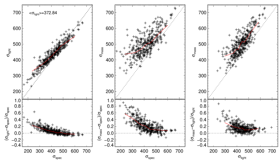
Figure 11: Comparison between dynamical and spectroscopic determinations of the velocity dispersion for all the cells with at least 1000 particles of one massive galaxy. The left-hand panels show the comparison between the dynamical velocity dispersion weighted by light, $\sigma_{light}$, and the spectroscopic velocity dispersion $\sigma_{spec}$. The middle panels show the comparison between the dynamical determination of the velocity dispersion weighted by mass , $\sigma_{mass}$, and the spectroscopic one, whereas the right-hand panels show the comparison between the two dynamical estimates, $\sigma_{mass}$ and $\sigma_{light}$. All the three projections of the galaxy are shown. The upper panels show the velocity dispersion comparisons whereas the bottom ones display the residuals. Each cross is a single determination in one cell. The dotted lines indicate the one to one relation and the red solid lines show the median values computed in equally populated intervals of velocity dispersion.

Figure 12: Comparison between dynamical and spectroscopic average velocity dispersions within one effective radius of the massive galaxies in our sample at z=0. Galaxies in all the three projections are shown. The upper panels show the comparisons between the velocity dispersions whereas the bottom ones display the residuals. Red symbols indicate galaxies for which less than 10 cells have been used for computing the average. The dotted lines indicate the one to one relation.

References

- Agertz et al. (2007) Agertz O., et al., 2007, MNRAS, 380, 963
- Baldry et al. (2004) Baldry I. K., Glazebrook K., Brinkmann J., Ivezić Ž., Lupton R. H., Nichol R. C., Szalay A. S., 2004, ApJ, 600, 681
- Barnes & Hernquist (1992) Barnes J. E., Hernquist L., 1992, ARA&A, 30, 705
- Bender, Burstein, & Faber (1992) Bender R., Burstein D., Faber S. M., 1992, ApJ, 399, 462
- Blanton et al. (2003) Blanton M. R., et al., 2003, ApJ, 594, 186
- Bois et al. (2012) Bois M., et al., 2012, arXiv, arXiv:1201.0885
- Bournaud, Jog, & Combes (2005) Bournaud F., Jog C. J., Combes F., 2005, A&A, 437, 69
- Bournaud et al. (2011) Bournaud F., et al., 2011, ApJ, 730, 4
- Bressan et al. (2006) Bressan A., et al., 2006, ApJ, 639, L55
- Cappellari & Emsellem (2004) Cappellari M., Emsellem E., 2004, PASP, 116, 138
- Cappellari et al. (2006) Cappellari M., et al., 2006, MNRAS, 366, 1126
- Cappellari et al. (2007) Cappellari M., et al., 2007, MNRAS, 379, 418
- Cassata et al. (2011) Cassata P., et al., 2011, ApJ, 743, 96
- Cen (2011) Cen R., 2011, ApJ, 741, 99
- Cenarro et al. (2001) Cenarro A. J., Cardiel N., Gorgas J., Peletier R. F., Vazdekis A., Prada F., 2001, MNRAS, 326, 959
- Cenarro & Trujillo (2009) Cenarro A. J., Trujillo I., 2009, ApJ, 696, L43
- (17) Cid Fernandes R., Mateus A., Sodré L., Stasińska G., Gomes J. M., 2005, MNRAS, 358, 363
- Cimatti et al. (2008) Cimatti A., et al., 2008, A&A, 482, 21
- Cimatti et al. (2004) Cimatti A., et al., 2004, Natur, 430, 184
- Coccato, Gerhard, & Arnaboldi (2010) Coccato L., Gerhard O., Arnaboldi M., 2010, MNRAS, 407, L26
- Cox et al. (2006) Cox T. J., Dutta S. N., Di Matteo T., Hernquist L., Hopkins P. F., Robertson B., Springel V., 2006, ApJ, 650, 791
- Cox et al. (2008) Cox T. J., Jonsson P., Somerville R. S., Primack J. R., Dekel A., 2008, MNRAS, 384, 386
- Daddi et al. (2005) Daddi E., et al., 2005, ApJ, 626, 680
- Daddi et al. (2007) Daddi E., et al., 2007, ApJ, 670, 156
- Damjanov et al. (2011) Damjanov I., et al., 2011, ApJ, 739, L44
- Dekel et al. (2009) Dekel A., et al., 2009, Natur, 457, 451
- (27) de la Rosa, I. G., la Barbera, F., Ferreras, I., de Carvalho, R. R. 2011, MNRAS, 418, L74
- de Zeeuw et al. (2002) de Zeeuw P. T., et al., 2002, MNRAS, 329, 513
- Di Matteo et al. (2009) Di Matteo P., Pipino A., Lehnert M. D., Combes F., Semelin B., 2009, A&A, 499, 427
- Dubois et al. (2013) Dubois Y., Gavazzi R., Peirani S., Silk J., 2013, MNRAS, 433, 3297
- Eggen, Lynden-Bell, & Sandage (1962) Eggen O. J., Lynden-Bell D., Sandage A. R., 1962, ApJ, 136, 748
- Eisenstein & Hu (1998) Eisenstein D.J., Hu W., 1998, ApJ, 511, 5
- Emsellem et al. (2007) Emsellem E., et al., 2007, MNRAS, 379, 401
- Emsellem et al. (2011) Emsellem et al. 2011, MNRAS, 414, 888
- Font et al. (2011) Font A. S., McCarthy I. G., Crain R. A., Theuns T., Schaye J., Wiersma R. P. C., Dalla Vecchia C., 2011, MNRAS, 416, 2802
- Fontana et al. (2006) Fontana A., et al., 2006, A&A, 459, 745
- Gallazzi et al. (2005) Gallazzi A., Charlot S., Brinchmann J., White S. D. M., Tremonti C. A., 2005, MNRAS, 362, 41
- Glazebrook et al. (2004) Glazebrook K., et al., 2004, Natur, 430, 181
- Haart & Madau (1996) Haart F., Madau P., 1996, ApJ, 461, 20
- Hernquist (1992) Hernquist L., 1992, ApJ, 400, 460
- Hopkins et al. (2009) Hopkins P. F., Cox T. J., Dutta S. N., Hernquist L., Kormendy J., Lauer T. R., 2009, ApJS, 181, 135
- Johansson et al. (2009) Johansson, P. H., Naab, T., & Ostriker, J. P. 2009, ApJ, 697, L38
- Johansson, Naab, & Ostriker (2012) Johansson P. H., Naab T., Ostriker J. P., 2012, ApJ, 754, 115
- Jørgensen (1999) Jørgensen I., 1999, MNRAS, 306, 607
- Katz, Weinberg & Hernquist (1996) Katz N., Weinberg D., Hernquist L., 1996, ApJS, 105, 19
- Kaviraj et al. (2007) Kaviraj S., et al., 2007, ApJS, 173, 619
- Kennicutt (1998) Kennicutt, R.C., 1998, ApJ, 498, 541
- Kereš et al. (2009) Kereš D., Katz N., Fardal M., Davé R., Weinberg D. H., 2009, MNRAS, 395, 160
- Kereš et al. (2005) Kereš D., Katz N., Weinberg D. H., Davé R., 2005, MNRAS, 363, 2
- Kereš et al. (2012) Kereš D., Vogelsberger M., Sijacki D., Springel V., Hernquist L., 2012, MNRAS, 425, 2027
- Khochfar & Silk (2009) Khochfar S., Silk J., 2009, MNRAS, 397, 506
- Khochfar et al. (2011) Khochfar S., et al., 2011, MNRAS, 417, 845
- Kobayashi (2004) Kobayashi C., 2004, MNRAS, 347, 740
- Koleva et al. (2009) Koleva M., Prugniel P., Bouchard A., Wu Y., 2009, A&A, 501, 1269
- La Barbera et al. (2012) La Barbera F., Ferreras I., de Carvalho R. R., Bruzual G., Charlot S., Pasquali A., Merlin E., 2012, MNRAS, 426, 2300
- Lackner et al. (2012) Lackner C. N., Cen R., Ostriker J. P., Joung M. R., 2012, MNRAS, 425, 641
- Larson (1975) Larson R. B., 1975, MNRAS, 173, 671
- Marchesini et al. (2009) Marchesini D., van Dokkum P. G., Förster Schreiber N. M., Franx M., Labbé I., Wuyts S., 2009, ApJ, 701, 1765
- (59) Mármol-Queraltó E., Cardiel N., Sánchez-Blázquez P., Trager S. C., Peletier R. F., Kuntschner H., Silva D. R., Cenarro A. J., Vazdekis A., Gorgas J., 2009, ApJ, 705, L199
- Mihos & Hernquist (1994) Mihos J. C., Hernquist L., 1994, ApJ, 437, L47
- Mihos & Hernquist (1996) Mihos J. C., Hernquist L., 1996, ApJ, 464, 641
- Moster et al. (2010) Moster B. P., Somerville R. S., Maulbetsch C., van den Bosch F. C., Macciò A. V., Naab T., Oser L., 2010, ApJ, 710, 903
- Naab & Burkert (2003) Naab T., Burkert A., 2003, ApJ, 597, 893
- Naab, Jesseit, & Burkert (2006) Naab T., Jesseit R., Burkert A., 2006, MNRAS, 372, 839
- Naab et al. (2009) Naab, T., Johansson, P. H., & Ostriker, J. P. 2009, ApJ, 699, L178
- Noeske et al. (2007) Noeske K. G., et al., 2007, ApJ, 660, L43
- Ocvirk, Pichon, & Teyssier (2008) Ocvirk P., Pichon C., Teyssier R., 2008, MNRAS, 390, 1326
- Oser et al. (2010) Oser L., Ostriker J.P., Naab T., Johansson P.H., Burkert A. 2010, 725, 2312
- Peng et al. (2002) Peng C.Y. et al. 2002, AJ, 124, 266
- Pérez-González et al. (2008) Pérez-González P. G., et al., 2008, ApJ, 675, 234
- Planelles & Quilis (2010) Planelles S., Quilis V., 2010, A&A, 519, A94
- Quilis (2004) Quilis V., 2004, MNRAS, 352, 1426
- Ravindranath et al. (2004) Ravindranath S., et al., 2004, ApJ, 604, L9
- Renzini (2006) Renzini A., 2006, ARA&A, 44, 141
- Ricciardelli et al. (2010) Ricciardelli E., Trujillo I., Buitrago F., Conselice C. J., 2010, MNRAS, 406, 230
- Ricciardelli et al. (2012) Ricciardelli E., Vazdekis A., Cenarro A. J., Falcón-Barroso J., 2012, MNRAS, 424, 172
- Rodighiero et al. (2011) Rodighiero G., et al., 2011, ApJ, 739, L40
- Sánchez-Blázquez et al. (2006) Sánchez-Blázquez P., et al., 2006, MNRAS, 371, 703
- Sánchez-Blázquez et al. (2007) Sánchez-Blázquez, P., Forbes D. A., Strader J., Brodie J., Proctor R., 2007, MNRAS, 377, 759
- Sarzi et al. (2008) Sarzi M., et al., 2008, ASPC, 390, 218
- Scannapieco et al. (2012) Scannapieco C., et al., 2012, MNRAS, 423, 1726
- Sérsic (1968) Sérsic J.L., 1968, Atlas de Galaxias Australes, Observatorio Astronomico, Cordoba, Argentina
- Springel & Hernquist (2003) Springel V., Hernquist L., 2003, MNRAS, 339, 289
- Sutherland & Dopita (1993) Sutherland R., Dopita M. S., 1993, ApJS, 88, 253
- Theuns et al. (1998) Theuns T., Leonard A., Efstathiou G., Pearce F. R., Thomas P. A, 1998, MNRAS, 301, 478
- Tojeiro et al. (2011) Tojeiro R., Percival W. J., Heavens A. F., Jimenez R., 2011a, MNRAS, 413, 434
- Trager et al. (2000) Trager S. C., Faber S. M., Worthey G., González J. J., 2000, AJ, 120, 165
- Trujillo et al. (2007) Trujillo I., Conselice C. J., Bundy K., Cooper M. C., Eisenhardt P., Ellis R. S., 2007, MNRAS, 382, 109
- Yepes et al. (1997) Yepes G., Kates R., Khokhlov A., Klypin A., 1997, MNRAS, 284, 235
- Valdes et al. (2004) Valdes F., Gupta R., Rose J. A., Singh H. P., Bell D. J., 2004, ApJS, 152, 251
- Vazdekis et al. (2003) Vazdekis, A., Cenarro, A. J., Gorgas, J., Cardiel, N., Peletier, R. F., 2003, MNRAS, 340, 1317-1345
- Vazdekis et al. (2012) Vazdekis A., Ricciardelli E., Cenarro A. J., Rivero-González J. G., Díaz-García L. A., Falcón-Barroso J., 2012, MNRAS, 424, 157
- Vazdekis et al. (2010) Vazdekis A., Sánchez-Blázquez P., Falcón-Barroso J., Cenarro A. J., Beasley M. A., Cardiel N., Gorgas J., Peletier R. F., 2010, MNRAS, 404, 1639
- Vogelsberger et al. (2012) Vogelsberger M., Sijacki D., Kereš D., Springel V., Hernquist L., 2012, MNRAS, 425, 3024
- Whitaker et al. (2012) Whitaker K. E., van Dokkum P. G., Brammer G., Franx M., 2012, arXiv, arXiv:1205.0547
- Whitaker et al. (2013) Whitaker K. E., et al., 2013, ApJ, 770, L39
- Zolotov et al. (2009) Zolotov A., Willman B., Brooks A. M., Governato F., Brook C. B., Hogg D. W., Quinn T., Stinson G., 2009, ApJ, 702, 1058