LHC and Tevatron constraints on a $W^{\prime}$ model interpretation of the top quark forward-backward asymmetry

Abstract

Aspects of a flavor-changing $W^{\prime}$ model with right-handed couplings are addressed in this paper in light of Tevatron and LHC data. Our fit to the Tevatron top-quark forward-backward asymmetry and the $t\bar{t}$ inclusive cross section includes higher-order loop effects in the effective interaction. The higher order corrections change the best fit value of the $W^{\prime}$ effective coupling strength as a function of the $W^{\prime}$ mass. The consistency of the model is checked against the shape of the $t\bar{t}$ invariant mass distribution. We use these updated $W^{\prime}$ parameters to compute the expected contributions from $W^{\prime}t$ associated production and, for the first time, $W^{\prime}W^{\prime}$ pair production at the LHC. We do a full Monte Carlo simulation of the $t\bar{t}X$ final state, including interference between the $tW^{\prime}$ induced $t\bar{t}j$ process and the standard model $t\bar{t}j$ process. Interference effects are shown to be quantitatively important, particularly when the $W^{\prime}$ mass is large. The jet multiplicity distribution in $t\bar{t}~{}\rm{jet}$ production at 8 TeV constrains the $W^{\prime}$ model severely.

I Introduction

Searches by the ATLAS and CMS Collaborations CMS (2013a); ATL (2013) have placed significant limits on the possible masses and coupling strengths of new charged vector currents which couple to the third generation of quarks, generically called $W^{\prime}$ bosons Duffty and Sullivan (2012, 2013). While these measurements have constrained a wide selection of models that go beyond the standard model, there is a class of models that escapes the limits by suppressing all flavor-changing couplings, except between the first and third generation. This particular class, in which a right-handed $W^{\prime}$ boson couples a down quark to a top quark, has been proposed Cheung et al. (2009); Barger et al. (2010); Cao et al. (2010); Cheung and Yuan (2011); Shelton and Zurek (2011); Gresham et al. (2011a); Barger et al. (2011); Bhattacherjee et al. (2011); Craig et al. (2011); Gresham et al. (2011b); Chen et al. (2011); Krohn et al. (2011); Gresham et al. (2012a); Cao et al. (2012); Yan et al. (2012); Berger et al. (2011a); Knapen et al. (2012); Berger et al. (2012); Duffty et al. (2012); Adelman et al. (2013); Endo and Iwamoto (2013); Berger et al. (2013, 2011b) as a possible explanation for anomalous measurements of the forward-backward asymmetry in $t\bar{t}$ production ($A_{FB}^{t\bar{t}}$) by the CDF Aaltonen et al. (2013) and D0 Collaborations Abazov et al. (2011). In this paper we investigate whether the class of models with a $W^{\prime}$–$t$–$d$ coupling strength that is consistent with the Fermilab Tevatron anomaly can also be consistent with data from the CERN Large Hadron Collider (LHC).

In a previous publication Duffty et al. (2012) we considered the leading-order (LO) correction to the forward-backward asymmetry due to a new term in the Lagrangian of the form

$$\mathcal{L}=\frac{g}{\sqrt{2}}V^{\prime}_{td}\bar{d}\gamma^{\mu}P_{R}tW^{\prime}_{\mu}+{\mathrm{h.c.}},$$ (1)

where $g$ is numerically equal to the standard model SU(2)_L gauge interaction coupling constant, and $V^{\prime}_{td}$ weights the effective strength of the interaction. In that paper we used the first $0.7$ fb^-1 of data collected at 7 TeV by the ATLAS Collaboration ATL (2011) to conclude $tW^{\prime}$ production with a decay to $t\bar{t}j$ could be used to exclude much of the interesting parameter space, and that with 5 fb^-1 of data the entire parameter space might be excluded. This conclusion was subject to the caveat that the relevant parameter space was only determined at leading order.

Both the ATLAS and CMS Collaborations reproduced our initial analysis and published exclusion limits Chatrchyan et al. (2012a); Aad et al. (2012a). However, there are large interference effects between $tW^{\prime}$ production and $t\bar{t}j$ that were not considered in the experimental analyses. The relevance of these effects is increased by the large couplings necessary to explain the Tevatron anomaly, $g_{\mathrm{eff}}=gV^{\prime}_{td}\sim 1$. Large coupling leads to a large width of the $W^{\prime}$ boson, and changes the observable signal at the LHC.

In this paper we significantly improve our calculation of the relevant parameter space for the class of models that satisfies the $t\bar{t}$ forward-backward asymmetry $A_{FB}^{t\bar{t}}$ measured by the CDF Collaboration  Aaltonen et al. (2013) and the $t\bar{t}$ inclusive cross section. In Sec. II.1 we derive the contribution to $A_{FB}^{t\bar{t}}$ at next-to-leading order (NLO) from $W^{\prime}$ bosons. In Sec. II.2 we show that the range of effective couplings $g_{\mathrm{eff}}$ changes from LO to NLO. In Sec. III we discuss the contribution of $W^{\prime}$ bosons to $t\bar{t}+\mathrm{n}j$ at the LHC, including full interference effects, as well as the contribution of $W^{\prime}W^{\prime}$ production and decay. We show that a 20 fb^-1 measurement of $t\bar{t}+\mathrm{n}j$ by the CMS Collaboration at 8 TeV excludes the region of couplings $g_{\mathrm{eff}}$ consistent with the Tevatron anomaly. We summarize our results in Sec. IV. Within the mass range $200<m_{W^{\prime}}<1100$ GeV, values of the coupling strength $V^{\prime}_{td}$ large enough to accommodate $A_{FB}^{t\bar{t}}$ observed at the Tevatron are incompatible with a good fit to the multiplicity distribution at the LHC.

Before proceeding, we comment briefly on indirect constraints on this $W^{\prime}$ model from other than the collider observables we address here. A right-handed $W^{\prime}$ may be constrained by the ratio of rare $B$ decays at the $2\sigma$ level Chen et al. (2011). However, the reach in these measurements is limited by theoretical uncertainty in the matrix elements for $B$ decays Li et al. (2005). While additional constraints on low-mass $W^{\prime}$ bosons may be derived from atomic parity violation Gresham et al. (2012b), the direct production limit we present from collider data is needed to exclude this right-handed $W^{\prime}$ model.

II Tevatron physics

In this section, we consider the influence of the $W^{\prime}$ model on the $t\bar{t}$ inclusive total cross section and on the $t\bar{t}$ forward-backward asymmetry $A_{FB}^{t\bar{t}}$ at the Tevatron. We fit data on the cross section and $A_{FB}^{t\bar{t}}$ and determine the best fit region of the parameters $(m_{W^{\prime}},g_{R})$. Consistency with data on the $t\bar{t}$ invariant mass distribution is then checked.

II.1 Calculation of $\sigma_{t\bar{t}}$ and $A_{FB}^{t\bar{t}}$

Previous work Duffty et al. (2012); Berger et al. (2013) shows that the best fits to the Tevatron asymmetry $A_{FB}^{t\bar{t}}$ and the inclusive cross section yield generally large values of the effective coupling strength $g_{R}$, especially for heavy $W^{\prime}$ bosons which are not excluded by direct observation. Thus the $\mathcal{O}\left(\alpha_{R}\right)$ ($\alpha_{R}\equiv g^{2}_{R}V_{td}^{\prime 2}/\left(4\pi\right)$) effects might not be negligible. We discuss two places where $\mathcal{O}\left(\alpha_{R}\right)$ effects play a role. The first is the loop correction to the QCD vertex $q\bar{q}g$, illustrated in Fig. 1. We can express the renormalized QCD vertex as

$$-ig_{s}T^{a}_{ij}\biggl{[} \gamma^{\mu}\left(1+\frac{\alpha_{R}}{4\pi}F_{V}^{f}\right)+\gamma^{\mu}\gamma_{5}\frac{\alpha_{R}}{4\pi}G_{A}^{f}$$

$$+\frac{\left(\bar{p}-p\right)^{\mu}}{2m_{q}}\frac{\alpha_{R}}{4\pi}F_{M}^{f}+\left(\bar{p}+p\right)^{\mu}\gamma_{5}\frac{\alpha_{R}}{4\pi}G_{E}^{f}\biggr{]},$$ (2)

where $p$ ($\bar{p}$) is the momentum of the quark (antiquark), and $f$ is the flavor index. The coefficients are non-zero for $f=t,d$. Analytic results for $F_{V}^{f},G_{A}^{f}$ and $F_{M}^{f}$ can be found in Ref. Beenakker et al. (1994). Corrections to the total cross section which are proportional to $G_{E}^{f}$ are all of order $\mathcal{O}\left(\alpha_{R}^{4}\alpha_{S}^{2}\right)$ and highly suppressed. They do not contribute to $\sigma_{F}-\sigma_{B}$. Thus, we will not consider them in this work.

Figure 1: (a) and (b) illustrate the $W^{\prime}$ loop correction to the $d\bar{d}g$ vertex. (c) shows the $t\bar{t}$ contribution to the $W^{\prime}$ width.

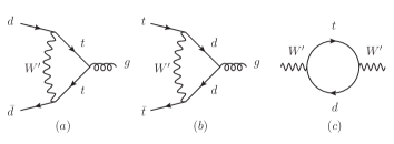
The additional contribution to $A_{FB}^{t\bar{t}}$ is

$$\sigma_{F}-\sigma_{B} = \frac{\alpha_{R}^{2}\alpha_{S}^{2}\beta^{2}{\mathrm{Re}}\left(G_{A}^{d}\right){\mathrm{Re}}\left(G_{A}^{t}\right)}{18\pi s}$$ (3)

$$+\mathcal{O}\left(\alpha_{R}^{3}\alpha_{S}^{2}\right),$$

where $\beta\equiv\sqrt{1-4m_{t}^{2}/s}$. The contribution to $A_{FB}^{t\bar{t}}$ from the QCD vertex correction has been investigated in Ref. Gabrielli and Raidal (2011).

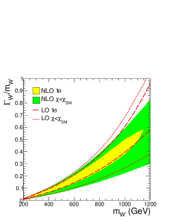
The decay width of the $W^{\prime}$ is another place where $\mathcal{O}\left(\alpha_{R}\right)$ effects are important for the LHC phenomenology of the $W^{\prime}$ model. The width is

$$\Gamma_{W^{\prime}}=\frac{\alpha_{R}m_{W^{\prime}}}{4}\left(1-r\right)\left(1+\frac{r}{2}\right)=\alpha_{R}\gamma\sim\mathcal{O}\left(\alpha_{R}\right),$$ (4)

where $r\equiv m_{t}^{2}/m_{W^{\prime}}^{2}$. A numerical evaluation is shown in Fig. 2.

Figure 2: The ratio of the width and the mass of the $W^{\prime}$ boson determined from the parameters of our best fits at the Tevatron. The values of $\chi^{2}$ in the light-shaded (yellow) region are not greater than 1. In the dark shaded (green) region they are not greater than the standard model (SM) value of $\chi^{2}$. For comparison, we show LO results when the $\mathcal{O}\left(\alpha_{R}\right)$ contributions are not included: Between the (red) dashed lines, $\chi^{2}$ is not greater than 1, and between the (red) dotted line $\chi^{2}$ is not greater than its SM value.

The standard model (SM) and new physics (NP) amplitudes are

$$\mathcal{M}_{SM}\equiv\frac{\mathcal{M}_{SM}^{(0)}+\alpha_{R}\mathcal{M}_{SM}^{(1)}}{s},$$ (5)

and

$$\mathcal{M}_{NP}\equiv\frac{\alpha_{R}\mathcal{M}_{NP}^{(1)}}{t-m_{W^{\prime}}^{2}+i\Gamma_{W^{\prime}}m_{W^{\prime}}}.$$ (6)

To $\mathcal{O}\left(\alpha_{R}^{2}\right)$ in the numerator, the interference term is

$$2\mathrm{Re}\left(\mathcal{M}_{NP}\mathcal{M}_{SM}^{*}\right) = \frac{2\alpha_{R}\mathcal{M}_{NP}^{(1)}\left(t-m_{W^{\prime}}^{2}\right)}{s\left[\left(t-m_{W^{\prime}}^{2}\right)^{2}+\alpha_{R}^{2}\gamma^{2}\right]}$$ (7)

$$\times{\mathrm{Re}}\left(\mathcal{M}_{SM}^{(0)}+\alpha_{R}\mathcal{M}_{SM}^{(1)}\right).$$

For the new physics term $\mathcal{M}_{NP}^{*}\mathcal{M}_{NP}$, it suffices to replace $\left(t-m_{W^{\prime}}^{2}\right)$ with $\left(t-m_{W^{\prime}}^{2}+i\Gamma_{W^{\prime}}m_{W^{\prime}}\right)$ to include the finite width effect.

After including the $\mathcal{O}\left(\alpha_{R}\right)$ correction to the QCD vertex, the non-zero helicity amplitudes can be written as $\mathcal{M}\left(\lambda_{q},\lambda_{\bar{q}},\lambda_{t},\lambda_{\bar{t}}\right)=4\pi\alpha_{S}t^{a}_{c_{3}c_{4}}t^{a}_{c_{2}c_{1}}\mathcal{M}_{SM}^{\left(\lambda_{q},\lambda_{\bar{q}},\lambda_{t},\lambda_{\bar{t}}\right)}+4\pi\alpha_{R}\delta_{c_{3}c_{1}}\delta_{c_{4}c_{2}}\mathcal{M}_{NP}^{\left(\lambda_{q},\lambda_{\bar{q}},\lambda_{t},\lambda_{\bar{t}}\right)}$, where

$$\mathcal{M}_{SM}^{\left(+-++\right)} = -\biggl{[}1+\frac{\alpha_{R}}{4\pi}\left(F_{V}^{t}+F_{V}^{q}+G_{A}^{q}+\frac{\beta^{2}F_{M}^{t}}{1-\beta^{2}}\right)$$ (8)

$$+\left(\frac{\alpha_{R}}{4\pi}\right)^{2}\left(F_{V}^{q}+G_{A}^{q}\right)\left(F_{V}^{t}+\frac{\beta^{2}F_{M}^{t}}{1-\beta^{2}}\right)\biggr{]}$$

$$\times\sqrt{1-\beta^{2}}\sin\theta,$$

$$\mathcal{M}_{SM}^{\left(-+++\right)} = -\biggl{[}1+\frac{\alpha_{R}}{4\pi}\left(F_{V}^{t}+F_{V}^{q}-G_{A}^{q}+\frac{\beta^{2}F_{M}^{t}}{1-\beta^{2}}\right)$$ (9)

$$+\left(\frac{\alpha_{R}}{4\pi}\right)^{2}\left(F_{V}^{q}-G_{A}^{q}\right)\left(F_{V}^{t}+\frac{\beta^{2}F_{M}^{t}}{1-\beta^{2}}\right)\biggr{]}$$

$$\times\sqrt{1-\beta^{2}}\sin\theta,$$

$$\mathcal{M}_{SM}^{\left(+-+-\right)} = -\biggl{[}1+\frac{\alpha_{R}}{4\pi}\left(F_{V}^{t}+F_{V}^{q}+G_{A}^{q}+\beta G_{A}^{t}\right)$$ (10)

$$+\left(\frac{\alpha_{R}}{4\pi}\right)^{2}\left(F_{V}^{q}+G_{A}^{q}\right)\left(F_{V}^{t}+\beta G_{A}^{t}\right)\biggr{]}$$

$$\times\left(1+\cos\theta\right),$$

$$\mathcal{M}_{SM}^{\left(-++-\right)} = \biggl{[}1+\frac{\alpha_{R}}{4\pi}\left(F_{V}^{t}+F_{V}^{q}-G_{A}^{q}+\beta G_{A}^{t}\right)$$ (11)

$$+\left(\frac{\alpha_{R}}{4\pi}\right)^{2}\left(F_{V}^{q}-G_{A}^{q}\right)\left(F_{V}^{t}+\beta G_{A}^{t}\right)\biggr{]}$$

$$\times\left(1-\cos\theta\right),$$

$$\mathcal{M}_{SM}^{\left(+--+\right)} = \biggl{[}1+\frac{\alpha_{R}}{4\pi}\left(F_{V}^{t}+F_{V}^{q}+G_{A}^{q}-\beta G_{A}^{t}\right)$$ (12)

$$+\left(\frac{\alpha_{R}}{4\pi}\right)^{2}\left(F_{V}^{q}+G_{A}^{q}\right)\left(F_{V}^{t}-\beta G_{A}^{t}\right)\biggr{]}$$

$$\times\left(1-\cos\theta\right),$$

$$\mathcal{M}_{SM}^{\left(-+-+\right)} = -\biggl{[}1+\frac{\alpha_{R}}{4\pi}\left(F_{V}^{t}+F_{V}^{q}-G_{A}^{q}-\beta G_{A}^{t}\right)$$ (13)

$$+\left(\frac{\alpha_{R}}{4\pi}\right)^{2}\left(F_{V}^{q}-G_{A}^{q}\right)\left(F_{V}^{t}-\beta G_{A}^{t}\right)\biggr{]}$$

$$\times\left(1+\cos\theta\right),$$

$$\mathcal{M}_{SM}^{\left(+---\right)} = \biggl{[}1+\frac{\alpha_{R}}{4\pi}\left(F_{V}^{t}+F_{V}^{q}+G_{A}^{q}+\frac{\beta^{2}F_{M}^{t}}{1-\beta^{2}}\right)$$ (14)

$$+\left(\frac{\alpha_{R}}{4\pi}\right)^{2}\left(F_{V}^{q}+G_{A}^{q}\right)\left(F_{V}^{t}+\frac{\beta^{2}F_{M}^{t}}{1-\beta^{2}}\right)\biggr{]}$$

$$\times\sqrt{1-\beta^{2}}\sin\theta,$$

$$\mathcal{M}_{SM}^{\left(+---\right)} = \biggl{[}1+\frac{\alpha_{R}}{4\pi}\left(F_{V}^{t}+F_{V}^{q}-G_{A}^{q}+\frac{\beta^{2}F_{M}^{t}}{1-\beta^{2}}\right)$$ (15)

$$+\left(\frac{\alpha_{R}}{4\pi}\right)^{2}\left(F_{V}^{q}-G_{A}^{q}\right)\left(F_{V}^{t}+\frac{\beta^{2}F_{M}^{t}}{1-\beta^{2}}\right)\biggr{]}$$

$$\times\sqrt{1-\beta^{2}}\sin\theta.$$

The symbol $\theta$ denotes the angle between the 3-momentum of the initial state quark and the final state top quark in the center-of-mass frame. Explicit expressions for the new physics amplitudes are

$$\mathcal{M}_{NP}^{\left(+-++\right)} = \frac{\left(1-\beta^{2}+8r_{W^{\prime}}\right)\sqrt{1-\beta^{2}}\sin\theta}{8r_{W^{\prime}}\left(1+\beta^{2}-2\beta\cos\theta+4r_{W^{\prime}}\right)},$$ (16)

$$\mathcal{M}_{NP}^{\left(+-+-\right)} = \frac{\left[\left(1-\beta\right)^{2}+8r_{W^{\prime}}\right]\left(1+\beta\right)}{8r_{W^{\prime}}\left(1+\beta^{2}-2\beta\cos\theta+4r_{W^{\prime}}\right)}$$ (17)

$$\times\left(1+\cos\theta\right),$$

$$\mathcal{M}_{NP}^{\left(+--+\right)} = -\frac{\left[\left(1+\beta\right)^{2}+8r_{W^{\prime}}\right]\left(1-\beta\right)}{8r_{W^{\prime}}\left(1+\beta^{2}-2\beta\cos\theta+4r_{W^{\prime}}\right)}$$ (18)

$$\times\left(1-\cos\theta\right),$$

$$\mathcal{M}_{NP}^{\left(+---\right)} = -\frac{\left(1-\beta^{2}+8r_{W^{\prime}}\right)\sqrt{1-\beta^{2}}\sin\theta}{8r_{W^{\prime}}\left(1+\beta^{2}-2\beta\cos\theta+4r_{W^{\prime}}\right)},$$ (19)

where $r_{W^{\prime}}\equiv m_{W^{\prime}}^{2}/s$. After integration over the azimuthal angle, the cross section can be written as

$$\frac{d\sigma}{d\cos\theta}=\frac{\beta}{32\pi s}\left(\frac{1}{2}\times\frac{1}{2}\times\frac{1}{3}\times\frac{1}{3}\right)\left|\mathcal{M}\right|^{2}.$$ (20)

We evaluate $\sigma_{t\bar{t}}$ and $A_{FB}^{t\bar{t}}$ using our analytic results for the squared amplitudes and the MSTW2008 parton distribution functions Martin et al. (2009). To include the NLO QCD and NNLO QCD contribution to $\sigma_{t\bar{t}}$ in the SM, and the NLO QCD SM contribution to $A_{FB}^{t\bar{t}}$, we remove the $\mathcal{O}\left(\alpha_{S}^{2}\alpha_{R}^{0}\right)$ portion of our result and substitute the NNLO QCD SM contribution for $\sigma_{t\bar{t}}$ and the NLO QCD term for $A_{FB}^{t\bar{t}}$. A complete NLO QCD calculation of this process is presented in Yan et al. (2012).

II.2 Fit to the Tevatron asymmetry data

Figure 3: Results of our fit to (a) the inclusive total cross section $\sigma_{t\bar{t}}$, and (b) the forward-backward asymmetry $A_{FB}^{t\bar{t}}$. In (c) we show the values of $\chi$ from our fit for a 1000 GeV $W^{\prime}$ boson. The light-shading (yellow) shows the 1$\sigma$ region from our combined fits. The dark-shading (green) shows the 2$\sigma$ region. The (black) solid line is the result with NLO vertex corrections included, while the (red) dashed line is the result without the NLO vertex corrections. The horizontal (blue) dashed lines in (a) and (b) denote the central values of the Tevatron data. The (blue) dotted line in (c) shows the value of $\chi$ for the SM.

Among the top quark observables at the Tevatron affected by the $W^{\prime}$ model contributions, we choose to determine our parameters from data on the inclusive cross section $\sigma_{t\bar{t}}$ and the asymmetry $A_{FB}^{t\bar{t}}$. We use the latest measurement of $\sigma_{t\bar{t}}$ at the Tevatron D0- (2012):

$$\sigma_{t\bar{t}}=7.65\pm 0.2~{}({\mathrm{stat.}})\pm 0.36~{}({\mathrm{syst.}})~{}{\mathrm{pb}}.$$ (21)

The corresponding (partial) NNLO SM QCD result is $7.24^{+0.24}_{-0.27}~{}{\mathrm{pb}}$, whereas our $\mathcal{O}\left(\alpha_{S}^{2}\alpha_{R}^{0}\right)$ result is $6.64$ pb. The latest measurement of the asymmetry from the CDF collaboration is $A_{FB}^{t\bar{t}}=(16.4\pm 4.7)\%$ Aaltonen et al. (2013) while the SM prediction (QCD+EW) is $(8.7\pm 1.0)\%$ Kuhn and Rodrigo (2012). For the calculation of $\chi^{2}$, we combine all these uncertainties treating them as uncorrelated.

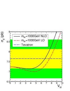
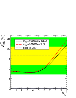
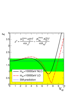
We use the result for a 1000 GeV $W^{\prime}$ as an example to show the effect of the vertex correction most clearly. As shown in Fig. 3(a), the vertex correction increases the predicted total cross section, making the best fit value of $V_{td}^{\prime}$ smaller than in the LO fits. The definition of $A_{FB}^{t\bar{t}}$

$$A_{FB}^{t\bar{t}}=\frac{\sigma_{F}-\sigma_{B}}{\sigma_{F}+\sigma_{B}}=\frac{\Delta\sigma}{\sigma_{\mathrm{tot}}},$$ (22)

shows that the corrections of $\Delta\sigma$ and $\sigma_{\mathrm{tot}}$ both contribute to the correction of $A_{FB}^{t\bar{t}}$. We have

$$A_{FB}^{t\bar{t}}\left(NLO\right) = \frac{\Delta\sigma+\delta\Delta\sigma}{\sigma_{\mathrm{tot}}+\delta\sigma_{\mathrm{tot}}}$$ (23)

$$\simeq A_{FB}^{t\bar{t}}\left(1+\frac{\delta\Delta\sigma}{\Delta\sigma}\right)\left(1-\frac{\delta\sigma_{\mathrm{tot}}}{\sigma_{\mathrm{tot}}}\right).$$

In the $W^{\prime}$ model, $\delta\Delta\sigma$ is of $\mathcal{O}\left(\alpha_{R}^{2}\alpha_{S}^{2}\right)$ which is tiny, and we see that $\delta\sigma_{\mathrm{tot}}$ is significant from Fig. 3(a). Thus the NLO $A_{FB}^{t\bar{t}}$ is smaller than the LO prediction (Fig. 3(b)).

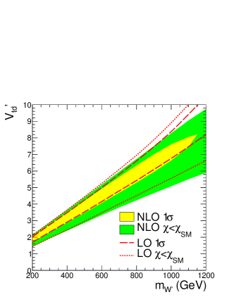
The values of $\chi$ from the combined fit to $\sigma_{t\bar{t}}$ and $A_{FB}^{t\bar{t}}$ are shown in Fig. 3(c) for $m_{W^{\prime}}=1$ TeV. Results for other values of the $W^{\prime}$ mass are qualitatively similar. In Fig. 4(a) we plot the allowed region $V^{\prime}_{td}$ as a function of the $W^{\prime}$ mass.

Figure 4: (a) The parameter $V^{\prime}_{td}$ obtained from our fits to $\sigma_{t\bar{t}}$ and $A_{FB}^{t}$ is shown as a function of the $W^{\prime}$ mass. (b) The coefficient $2\alpha_{R}m_{t}^{2}/\left(\alpha_{S}m_{W^{\prime}}^{2}\right)$ obtained from our fits is shown as a function of the $W^{\prime}$ mass. Values of $\chi^{2}$ in the light-shaded (yellow) region remain less than 1. Values of $\chi^{2}$ in the dark-shaded (green) region are not greater than the SM $\chi^{2}$. For comparison, we show the results without NLO $\mathcal{O}\left(\alpha_{R}\right)$ contributions: In the region between the (red) dashed lines $\chi^{2}$ is not greater than 1, and in the region between the (red) dotted lines $\chi^{2}$ is not greater than the SM $\chi^{2}$.

II.3 The $t\bar{t}$ mass distribution at the Tevatron

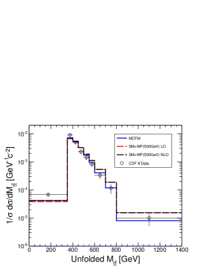
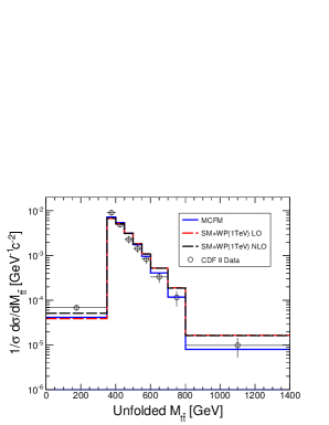
The distribution in the ${t\bar{t}}$ invariant mass at the Tevatron provides a potentially strong constraint on the $W^{\prime}$ model because the prediction of the $W^{\prime}$ model at high $m_{t\bar{t}}$ (last few bins of data) is much higher than the data Aaltonen et al. (2009). However, in Ref. Gresham et al. (2011b), the authors argue that it is not accurate to compare with the unfolded experimental result because there is a non-negligible difference between the cut acceptance in the $W^{\prime}$ model and the SM. This difference can reduce the tension between the $W^{\prime}$ model and data on the $m_{t\bar{t}}$ distribution.

In this work, we examine the consistency of our expectations with data on the distribution in $m_{t\bar{t}}$. We consider both the absolute cross section $d\sigma/dm_{t\bar{t}}$ and the mass distribution normalized by the integrated cross section. This latter shape distribution is arguably more pertinent because our parameters, determined from fits to data on the integrated cross section, already include information on the integrated cross section. We select two values of the $W^{\prime}$ mass and use the parameters from our best fit to compute the $m_{t\bar{t}}$ distribution. One value is a light $W^{\prime}$ ($m_{W^{\prime}}=500$ GeV, $g_{R}=3.8$), and the other is a heavy $W^{\prime}$ ($m_{W^{\prime}}=1000$ GeV, $g_{R}=7.0$).

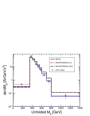
First, we compare the theoretical prediction with the unfolded Tevatron data (Fig. 5). Values of chi-squared per degree of freedom for the absolute cross section ($\chi^{2}/\mathrm{d.o.f.}$) and for the normalized distribution ($\chi_{N}^{2}/\mathrm{d.o.f.}$) are shown in Table 1. Compared with the unfolded data, the $W^{\prime}$ model prediction in the high $m_{t\bar{t}}$ region is not as good as the SM prediction, but the difference for a heavy $W^{\prime}$ is not sufficient to exclude a heavy $W^{\prime}$ from Tevatron data alone, $\chi^{2}/\mathrm{d.o.f.}=2.1$ in the $W^{\prime}$ case compared with $1.6$ in the SM. We note that a heavy $W^{\prime}$ boson fits the shape of the distribution (normalized distribution) better than it fits the absolute distribution, $\chi^{2}/\mathrm{d.o.f.}=2.1$ vs $\chi^{2}/\mathrm{d.o.f.}=3.6$. Moreover, the $W^{\prime}$ vertex correction relaxes the constraint from the shape of the $m_{t\bar{t}}$ distribution, $\chi^{2}/\mathrm{d.o.f.}=2.1$ vs $\chi^{2}/\mathrm{d.o.f.}=2.7$.

Figure 5: The $m_{t\bar{t}}$ distribution (upper two panels) and the normalized $m_{t\bar{t}}$ distribution (lower two panels) from the SM and the $W^{\prime}$ model. Left: ($m_{W^{\prime}}=500$ GeV, $g_{R}=3.8$); Right: ($m_{W^{\prime}}=1000$ GeV, $g_{R}=7.0$). The (blue) solid line is the SM NLO QCD prediction obtained from the MCFM Campbell et al. (2013) code. The lighter dashed (red) line shows the $W^{\prime}$ model prediction without the NLO vertex correction, and the darker dashed (black) line shows the $W^{\prime}$ model prediction with the NLO vertex correction included. The pure SM part of the $W^{\prime}$ model prediction is corrected to the NLO QCD level. The circles denote the Tevatron data along with their uncertainties.

Table 1: Chi squared per degree of freedom for the $m_{t\bar{t}}$ distribution at the Tevatron.

	$\chi^{2}/\mathrm{d.o.f.}$	$\chi_{N}^{2}/\mathrm{d.o.f.}$
SM	1.6	1.6
500 GeV $W^{\prime}$ (LO)	3.7	2.8
500 GeV $W^{\prime}$ (NLO)	3.8	2.6
1 TeV $W^{\prime}$ (LO)	3.4	2.7
1 TeV $W^{\prime}$ (NLO)	3.6	2.1

Before turning to constraints from LHC data, we consider the role of the difference in cut acceptance between the SM and the $W^{\prime}$ model Gresham et al. (2011b). This difference arises partially because the angular distribution of the top quark in the $W^{\prime}$ model behaves like $\left(1+\cos\theta\right)^{2}$, wheres in the SM it behaves like $\left(1+\cos^{2}\theta\right)$. More top quarks are expected in the large (positive) rapidity region in the $W^{\prime}$ case compared with the SM. The charged lepton from the top-quark decay will have nearly the same rapidity for an energetic top-quark owing to the right-handed coupling of the $W^{\prime}$ model Krohn et al. (2011); Berger et al. (2011a, 2012, 2013). On the other hand, these events will be suppressed by the small charged-lepton rapidity cut $|\eta_{\ell}|<1.0$ at Tevatron.

A simple analytic analysis is helpful for understanding the behavior of the cut acceptance. In the large $m_{t\bar{t}}$ region, $\beta\to 0$, and the squared-amplitude from the $d\bar{d}$ initial state behaves as

$$\propto \left(1+\cos^{2}\theta\right)-\frac{\alpha_{R}s}{2\alpha_{S}m_{W^{\prime}}^{2}}\frac{\left(1+\cos\theta\right)^{2}}{1+\frac{s}{2m_{W^{\prime}}^{2}}\left(1-\cos\theta\right)}$$ (24)

$$+\frac{9}{8}\left(\frac{\alpha_{R}s}{2\alpha_{S}m_{W^{\prime}}^{2}}\right)^{2}\frac{\left(1+\cos\theta\right)^{2}}{\left[1+\frac{s}{2m_{W^{\prime}}^{2}}\left(1-\cos\theta\right)\right]^{2}}.$$

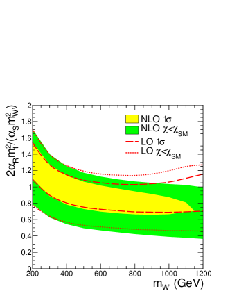
We show the $W^{\prime}$ mass dependence of $\alpha_{R}s/\left(2\alpha_{S}m_{W^{\prime}}^{2}\right)$ for $s=4m_{t}^{2}$ in Fig. 4(b). Using parameters from our best fits, we see that the coefficient is nearly independent of the mass of the $W^{\prime}$. It depends primarily on the center mass energy. Since the quadratic term gives a positive contribution which grows faster than the linear term, the contribution from the $W^{\prime}$ model is more significant in the large $m_{t\bar{t}}$ region than in the small $m_{t\bar{t}}$ region (c.f., Fig. 5).

To illustrate the effects of cut acceptance, we perform a simple parton level simulation whose results are shown Fig. 6. We use MadGraph5/MadEvent Alwall et al. (2011) to generate parton level $t\bar{t}$ events and decay the (anti-)top-quarks respecting their helicity information. We include the following energy smearing effects for jets

$$\frac{\delta E}{E}=0.1\oplus\frac{1}{\sqrt{E_{T}/{\mathrm{GeV}}}},$$ (25)

and charged leptons

$$\frac{\delta E}{E}=0.02\oplus\frac{0.135}{\sqrt{E_{T}/{\mathrm{GeV}}}}.$$ (26)

The $b$-tagging efficiency is taken from PGS4 Conway et al. (2013) as a function of the transverse energy and the rapidity of the $b$-quark. The difference between the cut acceptances of the SM and the $W^{\prime}$ model partially protects the $W^{\prime}$ model from the constraints of the $m_{t\bar{t}}$ distribution for a 500 GeV $W^{\prime}$. However, the difference is not great for a heavy $W^{\prime}$. We also checked the contribution from the $t\bar{t}j$ final state and found it to be negligibly small at the Tevatron as expected.

Figure 6: The cut acceptance for $t\bar{t}$ events as a function of $m_{t\bar{t}}$. The solid (black) line is the SM value. Acceptances in the $W^{\prime}$ model are shown for a 500 GeV $W^{\prime}$ dotted (red) line, and a 1 TeV $W^{\prime}$ dashed (blue) line.

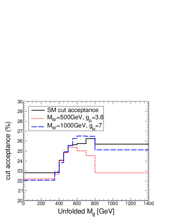
The message we draw is that while the shape of the invariant mass distribution favors the pure SM relative to a model that includes a $W^{\prime}$, this constraint is not decisive with Tevatron data.

Figure 7: Normalized cross section as a function of jet-multiplicity for jets with (a) $p_{T}>30$ GeV, (b) $p_{T}>60$ GeV, and (c) $p_{T}>100$ GeV. The data are from the CMS collaboration CMS (2013b). The dashed (red) lines are the results of the simulation shown in the CMS paper, whereas the solid (black) line is our simulation.

III $W^{\prime}$ and $t\bar{t}j$ at LHC

Having determined parameters of the $W^{\prime}$ model that are consistent with Tevatron data, we turn to an examination of the viability of the model at the LHC. We use data on the multiplicity of jets in $t\bar{t}$ events as our principal observable. In the $W^{\prime}$ model, the associated production of a top-quark and a $W^{\prime}$, with $W^{\prime}\rightarrow d\bar{t}$ contributes to the jet multiplicity along with SM QCD production of $t\bar{t}+\mathrm{n}j$. This contribution was proposed in Knapen et al. (2012); Duffty et al. (2012); Endo and Iwamoto (2013) and studied in data at 7 TeV Chatrchyan et al. (2012a); Aad et al. (2012a). We pay particular attention to the region of large $W^{\prime}$ mass where the coupling strength $g_{R}$ and $W^{\prime}$ width are large (c.f., Fig. 2). Owing to the broad width, interference between the amplitudes for $tW^{\prime}$ associated production and SM production of $t\bar{t}+j$ is not negligible Duffty et al. (2012); Endo and Iwamoto (2013). Interference has not yet been included in experimental analyses Chatrchyan et al. (2012a); Aad et al. (2012a). In this study, we also include for the first time the contribution to the jet multiplicity distribution in $t\bar{t}+\mathrm{n}j$ from $W^{\prime}$ pair production with, again, $W^{\prime}\rightarrow d\bar{t}$. It is important to include all of the contributions from the $W^{\prime}$ model to achieve a good estimation of the jet-multiplicity. In particular, the $t$-channel $W^{\prime}$ exchange process has a non-negligible influence on the $t\bar{t}+0j$ cross section.

III.1 Normalized jet-multiplicity

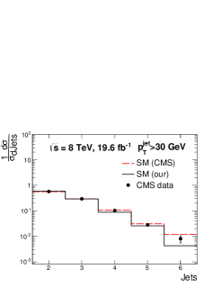
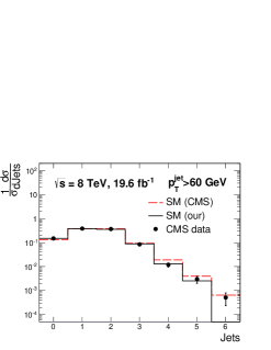
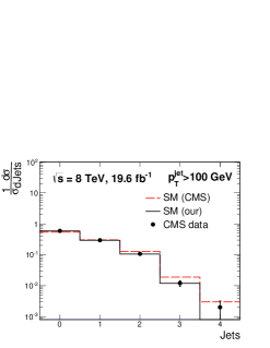
The normalized jet-multiplicity distribution in $t\bar{t}+X$ events is presented by the CMS collaboration in Figure 2 of their paper CMS (2013b). Our first task is to verify the accuracy of our simulation of SM $t\bar{t}+X$ production by comparing our simulation with that of CMS. We generate parton level $t\bar{t}+{\mathrm{n}}~{}j$ events to n$=2$ using MadGraph5/MadEvent Alwall et al. (2011). The generated events are subsequently processed with PYTHIA6.4 Sjostrand et al. (2006) for fragmentation and hadronization using the MLM prescription Mangano et al. (2007) for matching of jets with parton showers. We perform a detector simulation using the PGS4 code Conway et al. (2013).

Following the CMS cuts, muon candidates are required to have a transverse momentum $p_{T}>20$ GeV within a pseudorapidity region $|\eta|<2.4$ and to be isolated with $I_{\mathrm{rel}}<0.15$. The quantity $I_{\mathrm{rel}}$ is the sum of the transverse momenta of all neutral and charged reconstructed objects, except the muon itself, inside a cone of size $\Delta R\equiv\sqrt{\Delta\eta^{2}+\Delta\phi^{2}}<0.3$, divided by the muon transverse momentum. Electron candidates are required to have a transverse energy $E_{T}>20$ GeV within a pseudorapidity region $|\eta|<2.4$ and to be isolated with $I_{\mathrm{rel}}<0.15$. Jets are reconstructed using the anti-$k_{T}$ clustering algorithm with $R=0.5$ and required to have a transverse momentum $p_{T}>30$ GeV within a pseudorapidity region $|\eta|<2.4$. The PGS4 $b$-tagging Conway et al. (2013) efficiency is re-weighted to a maximum of 80% to mimic the $b$-tagging efficiency of CMS.

Signal events are required to have at least two isolated leptons with opposite electric charge (electrons or muons), and two jets, at least one of which is identified as a $b$-jet. Events with a lepton pair invariant mass smaller than 20 GeV are removed to suppress events from heavy flavor decays. In the $\mu^{+}\mu^{-}$ and $e^{+}e^{-}$ channels, the dilepton invariant mass is required to be outside a $Z$-boson mass window of $91\pm 15$ GeV, and the missing transverse energy $/{\!\!\!\!E}_{T}$ is required to be larger than 40 GeV.

Table 2: Standard model values of chi-squared for the normalized jet-multiplicity distribution in $t\bar{t}+X$ events at 8 TeV for different values of the jet transverse momentum cut.

	$p^{\mathrm{jet}}_{T}>30$ GeV	$p^{\mathrm{jet}}_{T}>60$ GeV	$p^{\mathrm{jet}}_{T}>100$ GeV
$\chi^{2}/{\mathrm{d.o.f}}$ (ours)	0.6	0.06	0.2
$\chi^{2}/{\mathrm{d.o.f}}$ (CMS)	0.2	1.6	4.5

Figure 8: (a) Example of standard model production of $t\bar{t}d$ production in a $dg$ interaction; (b) $W^{\prime}$ model production of $t\bar{t}d$; (c) $W^{\prime}$ exchange contribution to production of $t\bar{t}d$. Interference occurs between the processes (a) and (b), and between (a) and (c).

The results of our SM simulation are shown in Fig. 7 and compared with the CMS simulation and data. Our simulation agrees with the simulation by the CMS collaboration, and it agrees well with the data, except in the 6 jet bins at $p_{T}^{\rm jet}=30$ and $60$ GeV. We attribute this difference to the fact that we generate only up to $t\bar{t}+2j$ events at parton level. Thus, there are at most 4 jets in our parton level events. To calculate the value of $\chi^{2}$ of the SM simulation, we estimate the theoretical uncertainty from the differences between predictions obtained with different event generators and choices of hard scales CMS (2013b). Treating the experimental and theoretical uncertainties as uncorrelated, we obtain the values of the SM $\chi^{2}$ from our simulation shown in Table 2. The comparison of $\chi^{2}$ values shows that our simulation is as good as the CMS simulation. (For the samples with $p_{T}>60$ GeV and $p_{T}>100$ GeV, our values of ${\chi}^{2}$ are in fact better.)

Having established the reliability of our simulation code, we generate events from the $W^{\prime}$ model following the same method used for the SM events. At the parton level, we generate all $t\bar{t}+{\mathrm{n}}j$ processes including the interference between the SM $t\bar{t}+{\mathrm{n}}j$ process and inclusive $tW^{\prime}$ associated production. We generate parton level events to n=2. Examples of some of the processes that we compute are shown in Fig. 8. We remark that contributions from the $W^{\prime+}W^{\prime-}$ channel are also included. We examine the entire mass range $200<m_{W^{\prime}}<1100$ GeV, bearing in mind that a very light $W^{\prime}$ has been excluded in prior studies of Tevatron Aaltonen et al. (2012) and 7 TeV LHC data Chatrchyan et al. (2012a); Aad et al. (2012a). We are also aware that an extremely heavy $W^{\prime}$ (heavier than 1 TeV) is not consistent with the Tevatron $t\bar{t}$ observables (c.f., Fig. 4).

Figure 9: Normalized cross sections as a function of jet-multiplicity for jets with $p_{T}>30$ GeV (left panels), $p_{T}>60$ GeV (middle panels), and $p_{T}>100$ GeV (right panels). The figures in the upper row are the results for $m_{W^{\prime}}=500$ GeV and $V_{td}^{\prime}=4.195$. The figures in the lower row are the results for $m_{W^{\prime}}=1$ TeV and $V_{td}^{\prime}=6.634$. The (black) solid line is our SM simulation. The (blue) dotted lines represent our $W^{\prime}$ model results.

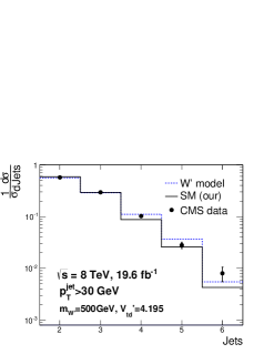
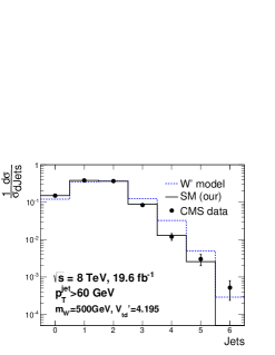
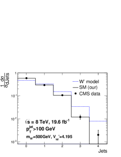
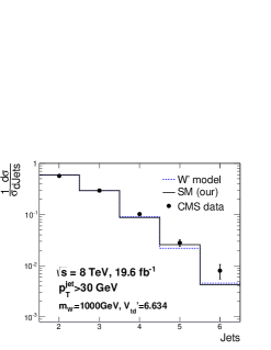
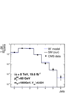
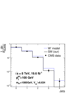
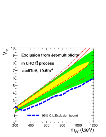
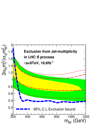
An examination of Fig. 9 shows qualitatively that the $W^{\prime}$ model agrees less well with the CMS normalized data than with the SM. In order to make this conclusion more quantitative for $W^{\prime}$ boson masses in the range $200<m_{W^{\prime}}<1100$ GeV, we perform fits in the space of $V^{\prime}_{td}$ vs $m_{W^{\prime}}$, and compute the resulting values of $\chi^{2}/{\mathrm{d.o.f}}$ in each bin of the normalized multiplicity distribution for each of the three values of $p^{\mathrm{jet}}_{T}>30$ GeV, $p^{\mathrm{jet}}_{T}>60$ GeV and $p^{\mathrm{jet}}_{T}>100$ GeV. In our calculation of $\chi^{2}/{\mathrm{d.o.f}}$ for $p^{\mathrm{jet}}_{T}>60$ GeV, we use only the bins with jet number up to 5, but including the 6 jet bin does not affect the final results. We use the set of $\chi^{2}$ values at each $W^{\prime}$ mass to determine the $95\%$ confidence level exclusion lines shown in Fig. 10. These results show that the $W^{\prime}$ model is disfavored by more than $2\sigma$ at the LHC if we use the parameter space determined in our fits to the Tevatron data and the $W^{\prime}$ boson is heavier than 300 GeV. In addition (not shown) most points in the best-fit region (light-shaded yellow region of Fig. 10) for explaining $A_{FB}^{t\bar{t}}$ at the Tevatron are excluded by 15–25$\sigma$.

Figure 10: (a) The 95% exclusion bound in the parameter space of $V^{\prime}_{td}$ vs $m_{W^{\prime}}$ from $\chi^{2}/{\mathrm{d.o.f}}$ fits to the LHC jet-multiplicity distribution in the inclusive $t\bar{t}X$ process at 8 TeV. The (blue) dashed line is the 95% exclusion bound. The dotted and dashed (red) lines and the light (yellow) and dark (green) shaded regions have the same meanings as those in Fig. 4. (b) The 95% exclusion bound shown for $2\alpha_{R}m_{t}^{2}/\left(\alpha_{S}m_{W^{\prime}}^{2}\right)$ vs $m_{W^{\prime}}$.

For light $W^{\prime}$ whose mass is $\sim 200$ GeV, the normalized jet-multiplicity is not a good observable for testing the $W^{\prime}$ model. For such a light $W^{\prime}$ boson, the narrow width approximation is good enough, and $tj$ resonance searches can be used at the LHC and the Tevatron Aaltonen et al. (2012); Chatrchyan et al. (2012a); Aad et al. (2012a).

III.2 Jet-multiplicity distribution:
Effects of interference and $W^{\prime}W^{\prime}$ pair-production

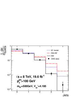
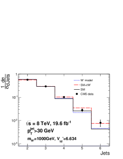
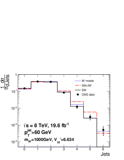
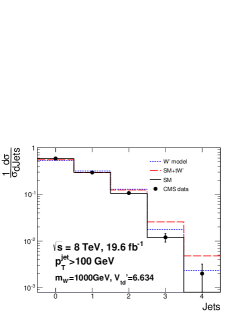
Both interference and $W^{\prime}W^{\prime}$ pair production contribute in each multiplicity bin. In order to isolate the effects from the interference of $tW^{\prime}$ associated production with SM $t\bar{t}+X$ production, and the effects from $W^{\prime+}W^{\prime-}$ pair production, we show figures in which we focus separately on each of these two contributions. We choose two values of $m_{W^{\prime}}$ with their associated values of $V_{td}^{\prime}$. Our benchmark points are $m_{W^{\prime}}=500$ GeV, $V_{td}^{\prime}=4.195$ and $m_{W^{\prime}}=1$ TeV and $V_{td}^{\prime}=6.634$, typical of a light $W^{\prime}$ and a heavy $W^{\prime}$, respectively. The results for $tW^{\prime}$ associated production without $W^{\prime}W^{\prime}$ pair-production are shown in Fig. 11.

Figure 11: The normalized distribution as a function of jet-multiplicity for jets with $p_{T}>30$ GeV (left panels), $p_{T}>60$ GeV (middle panels), $p_{T}>100$ GeV (right panels). The figures in the upper row are the results for $m_{W^{\prime}}=500$ GeV and $V_{td}^{\prime}=4.195$. The figures in the lower row are the results for $m_{W^{\prime}}=1$ TeV and $V_{td}^{\prime}=6.634$. The (red) dashed lines represent the results without the interference between $tW^{\prime}+X$ and SM $t\bar{t}+X$ production. The (blue) dotted lines are the results with interference included.

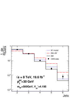
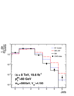
To obtain results that represent the incoherent sum of the SM and $tW^{\prime}$ processes, we generate parton-level $tW^{\prime}+{\mathrm{n}}j$ events to n$=1$, and decay the $W^{\prime}$ and $t$ ($\bar{t}$). Contributions from $t$-channel $W^{\prime}$ exchange processes are included when there is $W^{\prime}$ in the final state. After showering, hadronization, and event selection, we then add the SM $t\bar{t}+{\mathrm{n}}j$ contribution to the $tW^{\prime}+{\mathrm{n}}j$ result.

Our Fig. 11 shows that the difference between the incoherent SM+$tW^{\prime}$ result and the full $W^{\prime}$ model result is significant. There are two reasons for this difference. First, as $m_{W^{\prime}}$ increases, the width of the $W^{\prime}$ increases, and interference between the $tW^{\prime}$ and the SM $t\bar{t}+j$ processes grows in importance. Second, the full result contains the contribution from the $t$-channel $W^{\prime}$ exchange contribution to the $t\bar{t}$ production process, a contribution which is not small at the LHC. In Fig. 11 we see the complete $W^{\prime}$ model result is smaller than the incoherent SM+$tW^{\prime}$ result and that it agrees better with the data. Therefore, the strength of the signal may be overestimated if the incoherent sum of SM+$tW^{\prime}$ is used as an approximation.

Figure 12: The cross sections as a function of jet-multiplicity for jets with $p_{T}>30$ GeV (left panels), $p_{T}>60$ GeV (middle panels), $p_{T}>100$ GeV (right panels). The figures in the upper row are the results for $m_{W^{\prime}}=500$ GeV and $V_{td}^{\prime}=4.195$. The figures in the lower row are the results for $m_{W^{\prime}}=1$ TeV and $V_{td}^{\prime}=6.634$. The (red) dashed lines represent the results without the interference between the $tW^{\prime}+X$ and the SM $t\bar{t}+X$ production. The (blue) dotted lines are the results with interference included.

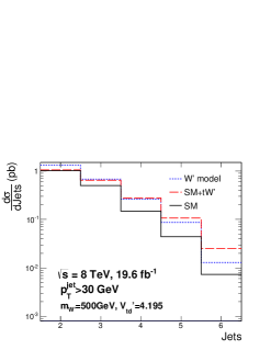
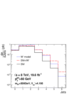
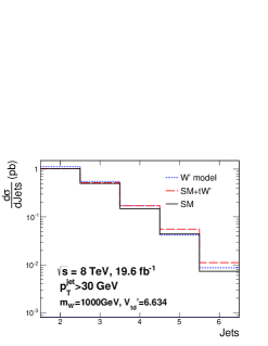
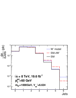
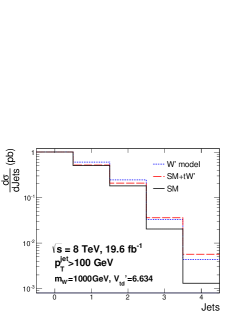
In Fig. 11 we present the normalized multiplicity distribution in order to compare with the CMS data CMS (2013b). On the other hand, the normalized distribution tends to obscure some features of the $W^{\prime}$ contribution and the effects of interference. In Fig. 12, we show instead the absolute cross sections as a function of jet multiplicity for the SM+$tW^{\prime}$ process. This figure shows that the incoherent sum of the SM+$tW^{\prime}$ processes is usually smaller than the complete calculation for $n_{\mathrm{jets}}\leqslant 3$, but it is larger than the result of the complete calculation for $n_{\mathrm{jets}}\geqslant 4$. Thus, for a light $W^{\prime}$ boson which has a relatively narrow width, including the interference effect in studies of data on $tj$ resonance searches will provide a stronger constraint on the $W^{\prime}$ model. For a heavy $W^{\prime}$ boson whose width is quite large, ignoring interference in fits to the normalized jet-multiplicity data in $t\bar{t}$ process, will lead to a constraint on the $W^{\prime}$ model that is too strong.

Figure 13: Cross sections as a function of jet-multiplicity for jets with $p_{T}>30$ GeV (left panels), $p_{T}>60$ GeV (middle panels), $p_{T}>100$ GeV (right panels). Results in the upper row are for $m_{W^{\prime}}=500$ GeV and $V_{td}^{\prime}=4.195$, whereas those in the lower row are for $m_{W^{\prime}}=1$ TeV and $V_{td}^{\prime}=6.634$. The (blue) dotted lines represent the complete calculation. The (sky blue) shadowed region is the contribution from the $W^{\prime}W^{\prime}$ pair production process.

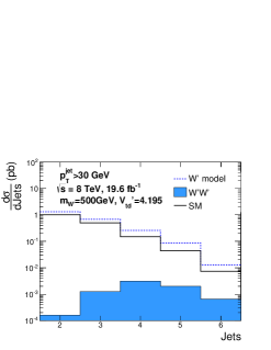
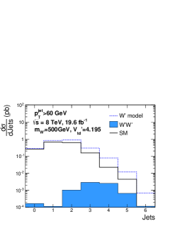
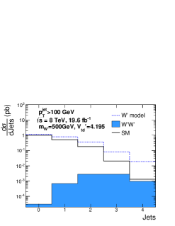
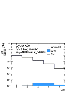
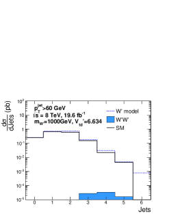
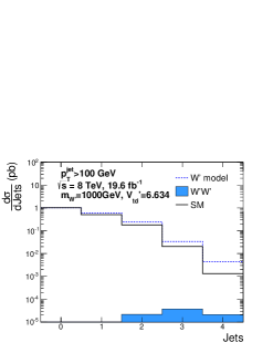
In Fig. 13, we show the absolute cross sections for the $W^{\prime}W^{\prime}$ pair production process. This process is mediated by top-quark exchange and is fed by the $d\bar{d}$ parton luminosity. Its contribution to the jet multiplicity distribution is typically several orders of magnitude smaller than the SM background, as seen in Fig. 13, becoming comparable when $n_{\mathrm{jets}}\geqslant 5$ for a light $W^{\prime}$ and large values of the $p^{\mathrm{jet}}_{T}$ cut. Overall, it is not an important component of the complete contribution from the $W^{\prime}$ model in the regions of parameter space explored in this paper.

IV Summary and conclusions

In this paper we investigate a model with right-handed coupling of a $W^{\prime}$ boson to the first and third quark generations. We fit for values of the coupling constant $V^{\prime}_{td}$ consistent with Tevatron data on the observed anomalously large top-quark forward-backward asymmetry $A_{FB}^{t\bar{t}}$ and $t\bar{t}$ cross section as a function of $W^{\prime}$ mass (c.f., Fig. 3). Our theoretical expressions include higher-order $W^{\prime}$ loop corrections whose contributions diminish the required best fit value of the coupling strength compared to previous LO fits.

Given the model and our determination of its parameters, we then investigate the consequences at the LHC. For masses of the $W^{\prime}$ below 400 GeV, our previous comparison to early ATLAS data excluded all relevant values of $V^{\prime}_{td}$ based on cross section rate Duffty et al. (2012). For larger masses, the predicted broader width of the $W^{\prime}$ requires other strategies, and we focus on the multiplicity distribution of jets accompanying a $t\bar{t}$ pair in the full 8 TeV CMS data sample. In the $W^{\prime}$ model, processes such as associated $tW^{\prime}$ production and $W^{\prime}W^{\prime}$ pair production, with $W^{\prime}\rightarrow\bar{t}d$, contribute to the $t\bar{t}+\mathrm{n}j$ final state along with standard model QCD production of $t\bar{t}+\mathrm{n}j$.

We simulate all $t\bar{t}+{\mathrm{n}}j$ processes including the interference between the SM $t\bar{t}+{\mathrm{n}}j$ process and inclusive $tW^{\prime}$ associated production; as well as contributions from the $W^{\prime+}W^{\prime-}$ channel. We examine the entire mass range $200<m_{W^{\prime}}<1100$ GeV. Our simulation includes parton fragmentation and hadronization from PYTHIA6.4 Sjostrand et al. (2006) and a detector simulation using the PGS code Conway et al. (2013). We compare our resulting jet multiplicity distribution with data from the CMS collaboration CMS (2013b). We show that interference plays a quantitatively significant role, altering the expected cross sections and exclusion bounds.

The essential conclusions of our study are shown in Fig. 10. Within the mass range $200<m_{W^{\prime}}<1100$ GeV, values of $V^{\prime}_{td}$ large enough to accommodate $A_{FB}^{t\bar{t}}$ observed at the Tevatron are incompatible with a good fit to the jet multiplicity distribution at the LHC.

There are other new physics models proposed for the top-quark $A_{FB}^{t\bar{t}}$ anomaly at Tevatron (for a more complete list of the references, cf. Ref. Duffty et al. (2012)). Many of them are disfavored or highly constrained by LHC data and other direct or indirect experiments. The most studied of these models are $t$-channel $W^{\prime}$ Cheung et al. (2009) and $Z^{\prime}$ Jung et al. (2010), and $s$-channel axigluon models Antunano et al. (2008). The $W^{\prime}$ model is disfavored by this work. The simplest $Z^{\prime}$ model is highly constrained by the same-sign top-quark search at the LHC Berger et al. (2011c); Aad et al. (2012b); Chatrchyan et al. (2012b). An updated $Z^{\prime}$ model in which the $Z^{\prime}$ boson is not self-conjugate Grinstein et al. (2011), so that there is no same-sign top-quark signal at colliders, would also be strongly constrained by $t\bar{t}+$jets data. A heavy axigluon is constrained by dijet and $t\bar{t}$ resonance searches at the LHC Berger et al. (2013). However, it is still possible that a light axigluon ($\sim 300$ GeV) could explain the $A_{FB}^{t\bar{t}}$ anomaly Gresham et al. (2013). Additional explanations involving multiple Higgs doublets Han et al. (2012); Wang and Han (2012) that are either composite Alvarez et al. (2011) or involve color-triplet scalars remain open.

The difficulties encountered in constructing models of new physics that can simultaneously accommodate the Tevatron asymmetry and LHC observables motivate inquiry into the standard model QCD expectations against which the data are compared. We note that a simple change of the renormalization scale brings the data and theory within $1\sigma$. This scale choice is similar to one that is used for the forward-backward asymmetry in $e^{-}e^{+}\to\mu^{-}\mu^{+}$ Brodsky and Wu (2012). We look forward to the next stage of fully differential NNLO calculations of $t\bar{t}$ production and decay that should be incorporated into the understanding of experimental acceptances, and allow for a full NLO prediction of $A_{FB}^{t\bar{t}}$ after cuts.