Generating Anisotropic Collapse and Expansion Solutions of Einstein’s Equations

Abstract

Analytic gravitational collapse and expansion solutions with anisotropic pressure are generated. Metric functions are found by requiring zero heat flow scalar. It emerges that a single function generates the anisotropic solutions. Each generating function contains an arbitrary function of time which can be chosen to fit various astrophysical time profiles. Two examples are provided: a bounded collapse metric and an expanding cosmological solution.
 
Keywords: anisotropic fluids, collapse, expansion

I INTRODUCTION

The general problem of anisotropic fluids which undergo spherical collapse with energy transport by heat flow was formulated some time ago by Misner and Sharp MS65 . General relativistic models with anisotropic stress have become increasing useful HOP08 ; HSW08 . There has been considerable interest in anisotropic spheres BL74 ; CHE+81 ; Bay82 ; Bon92 ; Via08 because of applications to stellar models DG02 ; DG04 ; MH03 ; ST12 . Collapse has been studied in the semiclassical regime by Visser et. al. BLSV08 . They found that Hawking radiation might prevent formation of a trapped surface and subsequent horizon, although an exponential approach might allow it to form in infinite time. They proposed a new class of collapsed objects with no horizons. (In this work, the collapse example does have a trapped surface.) Herrera and Santos HS97 have reviewed anisotropy in self-gravitating systems. Among the topics in their extensive review are discussions of the energy content of collapsing spheres and the stability of perturbed solutions. Herrera et. al. HOP08 mention the possibility of a single generating function for non-static anisotropic solutions. That possibility is developed in this work.

In previous work Gla81 , a method of generating collapse solutions with radial heat flow was presented. That method took a known spherical perfect fluid solution which was either static or in shear-free collapse and mapped it to a spherical shear-free collapse solution with radial heat flow. In this work, a different method of constructing anisotropic solutions is presented. The metric components are obtained by requiring zero heat flow scalar. A single function $R(t,r)$ and a parameter ”$\alpha$” generate anisotropic solutions. Not all ($\alpha,R$) pairs are allowed, since the $\alpha$ values are restricted. The fluid volume rate-of-expansion determines the type of anisotropic solution. There are two possibilities: collapse with shrinking volume and expansion with increasing volume.

The paper is organized as follows: section II describes the metric and metric functions. Section III covers energy-momentum components and treats the sectional curvature mass. Generated solutions are given in section IV. Section V has matching conditions which relate the interior and exterior. The work is summarized in section VI. Appendix A contains a general metric, an associated energy-momentum tensor with heat flow, and trapped surface equations.

II METRIC AND COMPONENTS

The collapse interior has an exterior which is vacuum Schwarzschild. Expanding interiors have cosmological exteriors. Both collapse and expanding interiors are covered by the spherically symmetric metric

$$g_{\mu\nu}^{\text{aniso}}dx^{\mu}dx^{\nu}=A^{2}dt^{2}-B^{2}dr^{2}-R^{2}d\Omega^{2}$$ (1)

where $A=A(t,r),B=B(t,r),R=R(t,r),$ and where $d\Omega^{2}$ is the metric of the unit sphere.

The velocity is comoving with $\hat{u}^{\mu}\partial_{\mu}=A^{-1}\partial_{t}$. The interior metric is spanned by the tetrad

$$\hat{u}_{\mu}dx^{\mu} =Adt,\ \ \hat{r}_{\mu}dx^{\mu}=Bdr,$$

$$\hat{\vartheta}_{\mu}dx^{\mu} =Rd\vartheta,\ \ \hat{\varphi}_{\mu}dx^{\mu}=R\text{sin}\vartheta d\varphi$$

such that

$$g_{\mu\nu}^{\text{aniso}}=\hat{u}_{\mu}\hat{u}_{\nu}-\hat{r}_{\mu}\hat{r}_{\nu}-\hat{\vartheta}_{\mu}\hat{\vartheta}_{\nu}-\hat{\varphi}_{\mu}\hat{\varphi}_{\nu}.$$ (2)

Metric components

Metric components are chosen so that the heat flow scalar $Q=0$. The equation for $Q$ is written from Eq.(51), where primes denote $\partial/\partial r$, and overdots denote $\partial/\partial t$, as

$$\frac{A^{\prime}}{A}\frac{\dot{R}}{R}+\frac{\dot{B}}{B}\frac{R^{\prime}}{R}-\frac{\dot{R}^{\prime}}{R}=0.$$ (3)

We find that,

$$A =h(t)\frac{\dot{R}}{R^{\alpha}},\text{ \ }h(t)\text{ arbitrary}$$ (4)

$$B =f(r)R^{\alpha},\text{ \ }f(r)\text{ arbitrary}$$ (5)

satisfies Eq.(3) identically for arbitrary $R(t,r)$. As a metric component $A=$ $h(t)\dot{R}/R^{\alpha}$ allows $h(t)$ to be absorbed by redefining $dt$, similarly for $f(r)$ and $dr$. Therefore we set $h(t)=f(r)=1$. The interior metric is now

$$g_{\mu\nu}^{\text{aniso}}dx^{\mu}dx^{\nu}=(\dot{R}/R^{\alpha})^{2}dt^{2}-R^{2\alpha}dr^{2}-R^{2}d\Omega^{2}.$$ (6)

Using values from Eqs.(4) and (5) for $A=\dot{R}/R^{\alpha}$ and $B=R^{\alpha}$, the fluid volume rate-of-expansion and rate-of-shear scalar, given in Eq.(49c) and Eq.(49d) respectively, are

$$\Theta =(\alpha+2)R^{\alpha-1}$$ (7)

$$\sigma =(1-\alpha)R^{\alpha-1}$$ (8)

thus restricting $\alpha:$  $\alpha\neq-2,1$. The value of $\Theta$ provides two different interiors: collapse with $\alpha<-2$ and expansion with $\alpha>1$.

We define a dimensionless measure of anisotropy as

$$\bigtriangleup a:=\frac{p_{r}-p_{\perp}}{p_{r}}.$$ (9)

III ENERGY-MOMENTUM AND MASS

The energy-momentum given in Appendix A is written here with zero heat flow $q^{\mu}$, since the heat scalar is chosen to vanish

$$T^{\mu\nu}=w\hat{u}^{\mu}\hat{u}^{\nu}+p_{r}\hat{r}^{\mu}\hat{r}^{\nu}+p_{\perp}(\hat{\vartheta}^{\mu}\hat{\vartheta}^{\nu}+\hat{\varphi}^{\mu}\hat{\varphi}^{\nu})$$ (10)

with fluid velocity $\hat{u}^{\mu}\hat{u}_{\mu}=1$ such that $\hat{u}^{\mu}\partial_{\mu}=A^{-1}\partial_{t}$. $w$ is the mass-energy density, $p_{r}$ is the radial pressure and $p_{\perp}$ is the tangential pressure.

Substituting in equations (53), (54), and (55) for $A=\dot{R}/R^{\alpha}$ and $B=R^{\alpha}$, we have

$$8\pi w=(1+2\alpha)R^{2\alpha-2}-\frac{1}{R^{2\alpha}}\left[2\frac{R^{\prime\prime}}{R}+(1-2\alpha)(\frac{R^{\prime}}{R})^{2}\right]+\frac{1}{R^{2}}$$ (11)

$$8\pi p_{r}=\frac{1}{R^{2\alpha}}\left[(2\alpha-1)(\frac{R^{\prime}}{R})^{2}-2\frac{\dot{R}^{\prime}}{\dot{R}}(\frac{R^{\prime}}{R})\right]+(1+2\alpha)R^{2\alpha-2}+\frac{1}{R^{2}}$$ (12)

$$8\pi p_{\perp} =-\alpha(1+2\alpha)R^{2\alpha-2}$$ (13)

$$+\frac{1}{R^{2\alpha}}\left[\frac{\dot{R}^{\prime\prime}}{\dot{R}}+(1-3\alpha)\frac{\dot{R}^{\prime}}{\dot{R}}(\frac{R^{\prime}}{R})+(1-\alpha)\frac{R^{\prime\prime}}{R}+\alpha(2\alpha-1)(\frac{R^{\prime}}{R})^{2}\right]$$

Specifying $R(t,r)$ and $\alpha$ distinguishes an anisotropic configuration.

Sectional Curvature Mass

Equation (52) provides the sectional curvature mass with $A=\dot{R}/R^{\alpha}$ and $B=R^{\alpha}$

$$\frac{2m}{R}=1+R^{2\alpha}-(R^{\prime})^{2}R^{-2\alpha}$$ (14)

When $R^{\prime}=R^{2\alpha}$ there is a possible trapped surface at $R=2m$. From equations (56) and (57) the trapping scalars are

$$\kappa_{1}=\frac{R^{\alpha}}{R}+\frac{R^{\prime}}{R^{\alpha+1}},\text{ \ }\kappa_{2}=\frac{R^{\alpha}}{R}-\frac{R^{\prime}}{R^{\alpha+1}}$$ (15)

When $\kappa_{1}$ and $\kappa_{2}$ have the same sign, a trapped surface will exist. For $R^{\prime}=R^{2\alpha}$ the trapping scalars are

$$\kappa_{1}=2R^{\alpha-1},\text{ \ }\kappa_{2}=0$$ (16)

They are both non-negative, therefore during collapse a trapped surface develops at $R=2m$. The trapped surface condition $R^{\prime}=R^{2\alpha}$ has the integral

$$R_{\text{trap}}^{1-2\alpha}=(1-2\alpha)r+H(t),\ H\text{ arbitrary}$$ (17)

When the trapped surface condition $R^{\prime}=R^{2\alpha}$ is substituted into equations (11,12,13) then

$$8\pi w=R_{\text{trap}}^{-2},\text{ \ }8\pi p_{r}=R_{\text{trap}}^{-2},\text{ \ }p_{\perp}\equiv 0.$$ (18)

IV Generated Solutions

(A) $\alpha=-5/2$

The rate-of-expansion must be negative for collapse, therefore $\alpha$ must be less than $-2$. Here we assume $\alpha=-5/2$. A trapped surface occurs when $R^{\prime}=R^{2\alpha}$. Thus $R^{\prime}=R^{-5}$ or $(R^{6})^{\prime}=6$ with solution

$$R_{\text{trap}}=[6r+h_{1}(t)]^{1/6},\text{ \ }h_{1}(t)\text{ arbitrary}$$ (19)

The density and pressure equations for $\alpha=-5/2$ become

$$8\pi w =-4R^{-7}-2R^{5}\left[\frac{R^{\prime\prime}}{R}+3(\frac{R^{\prime}}{R})^{2}\right]+R^{-2}$$ (20)

$$8\pi p_{r} =-2R^{5}\left[3(\frac{R^{\prime}}{R})^{2}+(\frac{R^{\prime}}{R})\frac{\dot{R}^{\prime}}{\dot{R}}\right]-4R^{-7}+R^{-2}$$ (21)

$$8\pi p_{\perp} =-10R^{-7}+R^{5}\left[\frac{\dot{R}^{\prime\prime}}{\dot{R}}+\frac{17}{2}\frac{\dot{R}^{\prime}}{\dot{R}}(\frac{R^{\prime}}{R})+\frac{7}{2}\frac{R^{\prime\prime}}{R}+15(\frac{R^{\prime}}{R})^{2}\right]$$ (22)

We assume $R=k(6r+h_{1})^{1/6}.$ The density and pressures in this case are

$$8\pi w =4k^{5}(1-k^{-12})(6r+h_{1})^{-7/6}+k^{-2}(6r+h_{1})^{-1/3}$$ (23)

$$8\pi p_{r} =4k^{5}(1-k^{-12})(6r+h_{1})^{-7/6}+k^{-2}(6r+h_{1})^{-1/3}$$ (24)

$$8\pi p_{\perp} =10(k^{4}-1)(6r+h_{1})^{-7/6}.$$ (25)

The mass-energy density $w(r)$ is graphed below in Figure 1.

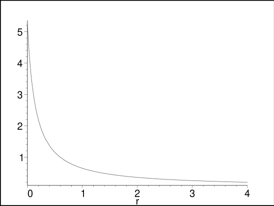
Figure 1: $k=2,$ $h_{1}(t)=1,$ w vs r  (unscaled)

When $k=1$ the density and pressures revert to the trapped values given in Eq.(18). The sectional curvature mass given in Eq.(14) is

$$2m_{1}(t,r)=R[1+(1-k^{2})R^{-5}]$$ (26)

The constant $k$ and function $h_{1}(t)$ remain free choices.

The dimensionless measure of anisotropy, defined in Eq.(9), is given by

$$\bigtriangleup a=1+\frac{10k^{2}(1-k^{4})}{4k^{7}(1-k^{-12})+(6r+h_{1})^{5/6}}$$ (27)

For $h_{1}(t)$ constant and fixed $k$, the anisotropy is a maximum at the center $r=0$. As $r$ increases $\bigtriangleup a$ falls to $1+\epsilon$ ($r$ has an upper bound - see the section on Matching). At the trapped surface, where $k=1$, there is a minimum with $\bigtriangleup a=1$.

(B) $\alpha=3/2$

We choose $\alpha=3/2$ with $\Theta=(5/2)R^{1/2}$ for expansion. We also choose

$$R=(r^{2}+r_{0}^{2})^{-1}+h_{2}(t),\text{ \ }h_{2}(t)\text{ arbitrary}$$ (28)

For $\alpha=3/2$

$$8\pi w =4R-2R^{-3}[\frac{R^{\prime\prime}}{R}-(\frac{R^{\prime}}{R})^{2}]+R^{-2}$$ (29)

$$8\pi p_{r} =2R^{-3}[(\frac{R^{\prime}}{R})^{2}-(\frac{R^{\prime}}{R})\frac{\dot{R}^{\prime}}{\dot{R}}]+4R+R^{-2}$$ (30)

$$8\pi p_{\perp} =-R[2\frac{\ddot{R}}{\dot{R}}(\frac{R}{\dot{R}})+3]+R^{-3}[\frac{\dot{R}^{\prime\prime}}{\dot{R}}-\frac{3}{2}(\frac{\dot{R}^{\prime}}{\dot{R}})(\frac{R^{\prime}}{R})-\frac{1}{2}\frac{R^{\prime\prime}}{R}+\frac{3}{4}(\frac{R^{\prime}}{R})^{2}]$$ (31)

With $F(t,r):=1+h_{2}(t)(r^{2}+r_{0}^{2})$ and $R=F/(r^{2}+r_{0}^{2})$, the density and pressures in this case are

$$8\pi w =\frac{4F}{r^{2}+r_{0}^{2}}+\frac{(r^{2}+r_{0}^{2})^{2}}{F^{2}}+\frac{4(r^{2}+r_{0}^{2})(r_{0}^{2}-3r^{2})}{F^{4}}+\frac{8r^{2}(r^{2}+r_{0}^{2})}{F^{5}}$$ (32)

$$8\pi p_{r} =\frac{4F}{r^{2}+r_{0}^{2}}+\frac{(r^{2}+r_{0}^{2})^{2}}{F^{2}}+\frac{8r^{2}(r^{2}+r_{0}^{2})}{F^{5}}$$ (33)

$$8\pi p_{\perp} =-\frac{F}{r^{2}+r_{0}^{2}}[2F\frac{\ddot{F}}{(\dot{F})^{2}}+3]+\frac{(r^{2}+r_{0}^{2})^{2}(r_{0}^{2}-3r^{2})}{F^{4}}-\frac{3r^{2}}{F^{2}(r^{2}+r_{0}^{2})^{2}}$$ (34)

Fig.2 $\ h_{2}(t)=1$, $r_{0}=1$,  w vs r  (unscaled)

The sectional curvature mass is

$$2m_{2}(t,r)=\frac{F}{r^{2}+r_{0}^{2}}\left[1+\frac{F^{3}}{(r^{2}+r_{0}^{2})^{3}}-\frac{4r^{2}}{(r^{2}+r_{0}^{2})F^{3}}\right].$$ (35)

When $h_{2}(t)=1$ and $r_{0}=1$, as in Figure 2, then as $r\rightarrow\infty$  $2m_{2}\rightarrow$ $2$.

V Matching

Interior and exterior regions match across a separating boundary $\Sigma$ if the first and second fundamental forms are continuous across $\Sigma$ MS93 . The collapsing interiors match to a Schwarzschild exterior

$$ds_{(+)}^{2}=(1-2m_{0}/\tilde{r})d\tilde{t}^{2}-(1-2m_{0}/\tilde{r})^{-1}d\tilde{r}^{2}-\tilde{r}^{2}d\Omega^{2}.$$ (36)

The interior metric is

$$ds_{(-)}^{2}=A^{2}dt^{2}-B^{2}dr^{2}-R^{2}d\Omega^{2}.$$ (37)

(Interior objects will be indicated by a minus and exterior objects by a plus.) The metric match requires

$$A =(1-2m_{0}/r_{\Sigma})^{1/2}$$ (38)

$$B =(1-2m_{0}/r_{\Sigma})^{-1/2}$$ (39)

$$R =r_{\Sigma}$$ (40)

At the boundary, the sectional curvature mass must equal the exterior Schwarzschild mass parameter

$$m(r_{\Sigma})=m_{0}$$ (41)

The unit normal to the boundary is

$$N_{\mu}dx^{\mu}=-(1-2m_{0}/r_{\Sigma})^{1/2}d\tilde{t}+\sqrt{2}(1-2m_{0}/r_{\Sigma})^{-1/2}d\tilde{r}$$ (42)

such that $g_{(+)}^{\mu\nu}N_{\mu}N_{\nu}=-1$

Junction conditions equivalent to continuity of the second fundamental form are

$$(G_{\mu\nu}N^{\mu}N^{\nu})_{{}^{\Sigma}}^{+}=(G_{\mu\nu}N^{\mu}N^{\nu})_{{}^{\Sigma}}^{-},$$ (43)

$$(G_{\mu\nu}N^{\mu}e_{{}^{j}}^{\nu})_{{}^{\Sigma}}^{+}=(G_{\mu\nu}N^{\mu}e_{{}^{j}}^{\nu})_{{}^{\Sigma}}^{-},$$ (44)

where three linearly independent $e_{{}^{j}}^{\nu}$ span the boundary surface. The Schwarzschild exterior is vacuum, so that

$$(G_{\mu\nu}N^{\mu}N^{\nu})_{{}^{\Sigma}}^{-} =0,$$

$$(G_{\mu\nu}N^{\mu}e_{{}^{j}}^{\nu})_{{}^{\Sigma}}^{-} =0.$$

This implies that at the boundary

$$(w)_{\Sigma}=(p_{r})_{\Sigma}=(p_{\perp})_{\Sigma}=0$$ (45)

i.e. the density and pressures must vanish. Figure 1 show the density falling off to zero. The pressures fall off similarly.

Expanding solutions have cosmological exteriors. Collins Col77 discussed the global properties of Kantowski-Sachs KS66 cosmologies. He dropped their dust condition and showed in detail how the expanding interiors relate to their cosmological exteriors.

VI SUMMARY

Analytic anisotropic collapse and expansion solutions have been generated. The interior collapse metric has been matched to an exterior Schwarzschild vacuum. The collapse solution has a trapped surface where the dimensionless anisotropy measure is minimized. To paraphrase Herrera and Santos HS97 : ”For dense systems, phase transitions may occur during gravitational collapse, particularly transitions to a pion condensed state. A softened equation of state can provide a large energy release which is important in the evolution of collapsing configurations.” Additionally, redshift data from the Coma cluster of galaxies GDK99 shows a distinct infall region.

Expanding solutions have been discussed by Collins Col77 . These solutions allow inhomogeneous cosmologies to be modelled. For instance, Barrow and Maartens BM98 have investigated the effect of anisotropic stresses on the late-time evolution of inhomogeneous universes. They found decay of shear anisotropy to be slowed by the presence of anisotropic stresses. They also found attractor solutions relating distortion in the expansion anisotropy to the fractional density in anisotropic stress.

This work differs from previous studies such as HOP08 ; BL74 ; CHE+81 ; DG02 ; MH03 which are static, and studies HPO01 in which the spherical area radius is simplified to $r$, rather than $R(t,r)$ used here. We find this is the only work which uses $R(t,r)$ to generate solutions. In summary, the solution generating function is $R(t,r)$ with parameter ”$\alpha$”. $R(t,r)$ was constructed by requiring zero heat flow scalar. For each valid choice of $\alpha$ and $R(t,r)$, one obtains an anisotropic configuration which collapses or expands, and each generating function contains an arbitrary function of time which can be chosen to fit various astrophysical time profiles.

ACKNOWLEDGMENT

We thank Professor Jean Krisch for constructive comments.

Appendix A Energy-Momentum and physical components

Metric

$$g_{\mu\nu}^{\text{aniso}}dx^{\mu}dx^{\nu}=A^{2}dt^{2}-B^{2}dr^{2}-R^{2}d\Omega^{2}$$

is Petrov type D. The two principal null vectors, normal to ($\vartheta,\varphi$) two-surfaces, are

$$l^{\mu}\partial_{\mu} =A^{-1}\partial_{t}+B^{-1}\partial_{r}$$ (46)

$$n^{\mu}\partial_{\mu} =A^{-1}\partial_{t}-B^{-1}\partial_{r}.$$ (47)

The energy-momentum tensor is given by ($G=c=1$)

$$T^{\mu\nu}=w\hat{u}^{\mu}\hat{u}^{\nu}+p_{r}\hat{r}^{\mu}\hat{r}^{\nu}+p_{\perp}(\hat{\vartheta}^{\mu}\hat{\vartheta}^{\nu}+\hat{\varphi}^{\mu}\hat{\varphi}^{\nu})+q^{\mu}\hat{u}^{\nu}+\hat{u}^{\mu}q^{\nu}$$ (48)

where $p_{r}$ is the radial pressure, $p_{\perp}$ is the tangential pressure, $w$ is the mass-energy density, and $q^{\mu}$ is the radial heat flow vector orthogonal to $\hat{u}^{\mu}$. We use notation of Taub Tau69 for $w$. Taub’s purpose was to distinguish mass-energy density from proper mass-density $\rho$, with $w=\rho(1+\epsilon)$. This allows the first law of thermodynamics to be written in its usual form $Tds=d\epsilon+pd(1/\rho)$ with specific entropy $s$ and specific internal energy $\epsilon$. The kinematics of the fluid are described by

$$\hat{u}_{\mu;\nu} =a_{\mu}\hat{u}_{\nu}+\sigma_{\mu\nu}-(\Theta/3)(\hat{r}_{\mu}\hat{r}_{\nu}+\hat{\vartheta}_{\mu}\hat{\vartheta}_{\nu}+\hat{\varphi}_{\mu}\hat{\varphi}_{\nu}),$$ (49a)

$$a_{\mu}dx^{\mu} =-(A^{\prime}/A)dr,$$ (49b)

$$\Theta =A^{-1}(\dot{B}/B+2\dot{R}/R),$$ (49c)

$$\sigma_{\mu\nu} =\sigma[-2\hat{r}_{\mu}\hat{r}_{\nu}+\hat{\vartheta}_{\mu}\hat{\vartheta}_{\nu}+\hat{\varphi}_{\mu}\hat{\varphi}_{\nu}],\ \ \sigma=A^{-1}(\dot{R}/R-\dot{B}/B)$$ (49d)

where primes denote $$\partial/\partial r \partial/\partial t \sigma_{\mu\nu} \sigma_{\mu\nu}\sigma^{\mu\nu}=6\sigma^{2} q^{\mu}\hat{u}_{\mu}=0$$, and overdots denote . The rate-of shear is trace-free, and . The heat flow vector () is given by

$$4\pi q^{\mu}\partial_{\mu} =Q\partial_{r}$$ (50)

$$Q =(AB)^{-1}\left[\frac{A^{\prime}}{A}\frac{\dot{R}}{R}+\frac{\dot{B}}{B}\frac{R^{\prime}}{R}-\frac{\dot{R}^{\prime}}{R}\right]$$ (51)

The sectional curvature mass is

$$2m=R^{3}R_{\alpha\beta\mu\nu}\hat{\vartheta}^{\alpha}\hat{\varphi}^{\beta}\hat{\vartheta}^{\mu}\hat{\varphi}^{\nu}=R[1+\dot{R}^{2}/A^{2}-(R^{\prime})^{2}/B^{2}].$$ (52)

The mass-energy density and pressures are given, respectively, by

$$8\pi w=\frac{1}{A^{2}}\left[(\frac{\dot{R}}{R})^{2}+2\frac{\dot{R}}{R}\frac{\dot{B}}{B}\right]-\frac{1}{B^{2}}\left[2\frac{R^{\prime\prime}}{R}+(\frac{R^{\prime}}{R})^{2}-2\frac{B^{\prime}}{B}\frac{R^{\prime}}{R}\right]+\frac{1}{R^{2}}$$ (53)

$$8\pi p_{r}=\frac{1}{B^{2}}\left[(\frac{R^{\prime}}{R})^{2}+2\frac{R^{\prime}}{R}\frac{A^{\prime}}{A}\right]-\frac{1}{A^{2}}\left[2\frac{\ddot{R}}{R}+(\frac{\dot{R}}{R})^{2}-2\frac{\dot{R}}{R}\frac{\dot{A}}{A}\right]-\frac{1}{R^{2}}$$ (54)

$$8\pi p_{\perp}=-\frac{1}{A^{2}}[\frac{\ddot{R}}{R}+\frac{\ddot{B}}{B}+\frac{\dot{R}}{R}(\frac{\dot{B}}{B}-\frac{\dot{A}}{A})+\frac{\dot{A}}{A}\frac{\dot{B}}{B}]+\frac{1}{B^{2}}[\frac{R^{\prime\prime}}{R}+\frac{A^{\prime\prime}}{A}+\frac{R^{\prime}}{R}(\frac{A^{\prime}}{A}-\frac{B^{\prime}}{B})-\frac{A^{\prime}}{A}\frac{B^{\prime}}{B}]$$ (55)

Trapped Surfaces

The topological two-spheres ($\vartheta,\varphi$) nested in an $R=const$ surface at time $t$ have outgoing null geodesic normal $l^{\mu}$ and incoming null geodesic normal $n^{\mu}$. The two principal null vectors (46) and (47) provide trapping scalars

$$\kappa_{1}=l^{\mu}\partial_{\mu}(\ln R),\text{ \ }\kappa_{2}=n^{\mu}\partial_{\mu}(\ln R).$$

When scalars Sen02 $\kappa_{1}$ and $\kappa_{2}$ have the same sign, a trapped surface Pen65 will exist:

$$\kappa_{1} =A^{-1}(\dot{R}/R)+B^{-1}(R^{\prime}/R)$$ (56)

$$\kappa_{2} =A^{-1}(\dot{R}/R)-B^{-1}(R^{\prime}/R).$$ (57)

References

(1)C.W. Misner and D.H. Sharp, Phys. Lett 15, 279 (1965).
Spherical Gravitational Collapse with Energy Transport by Radiative
Diffusion
(2)L. Herrera, J. Ospino and A. Di Prisco, Phys. Rev.
D 77, 027502 (2008). All static spherically symmetric
anisotropic solutions of Einstein’s equations
(3)L. Herrera, N.O. Santos and A. Wang, Phys. Rev. D 78, 084026 (2008). Shearing Expansion-free Spherical Anisotropic Fluid
Evolution
(4)R.L. Bowers and E.P.T. Liang, Astrophys. J. 188, 657
(1974). Anisotropic spheres in general relativity
(5)M. Cosenza, L. Herrera, M. Esculpi, and L. Witten, J. Math.
Phys. 22, 118 (1981). Some models of anisotropic spheres in
general relativity
(6)S.S. Bayin, Phys. Rev. D 26, 1262 (1982).
Anisotropic fluid spheres in general relativity
(7)H. Bondi, Mon. Not. Roy. Astr. Soc. 259, 365 (1992).
Anisotropic spheres in general relativity
(8)S. Viaggiu, Int. J. Mod. Phys. D18, 275 (2009).
Modeling Usual and Unsual Anisotropic Spheres
(9)K. Dev and M. Gleiser, Gen. Rel. Gravit. 34, 1793
(2002). Anisotropic stars: exact solutions
(10)K. Dev and M. Gleiser, Int. J. Mod. Phys. D13, 1389
(2004). Anisotropic Stars: Exact Solutions and Stability
(11)M.K. Mak and T. Harko, Proc. Roy. Soc. Lond. A 459,
393 (2003). Anisotropic Stars in General Relativity
(12)R. Sharma and R. Tikekar, Pramana J. Phys. 79, 501
(2012). Non-adiabatic radiative collapse of a relativistic star under
different initial conditions
(13)C. Barceló, S. Liberati, S. Sonego, and M. Visser, Phys.
Rev. D 77, 044032 (2008). Fate of gravitational collapse in
semiclassical gravity
(14)L. Herrera and N.O. Santos, Phys. Rep. 286, 53 (1997).
Local anisotropy in self-gravitating systems
(15)E.N. Glass, Phys. Lett. 86A, 351 (1981).
Shear-free Collapse With Heat Flow
(16)M. Mars and J.M.M. Senovilla, Class. Quantum Grav. 10,
1865 (1993). Geometry of general hypersurfaces in spacetime - junction
conditions.
(17)C.B. Collins, J. Math. Phys. 18, 2116 (1977).
Global structure of the ’Kantowski-Sachs’ cosmological models
(18)R. Kantowski and R.K. Sachs, J. Math. Phys. 7, 443
(1966). Some Spatially Homogeneous Anisotropic Relativistic
Cosmological Models
(19)M.J. Geller, A. Diaferio, and M.J. Kurtz, Astrophys. J.
517, L23 (1999). The Mass Profile of the Coma Galaxy Cluster
(20)J.D. Barrow and R. Maartens, Phys. Rev. D 59, 043502
(1998). Anisotropic Stresses in Inhomogeneous Universes
(21)A.H. Taub, Commun. Math. Phys. 15, 235 (1969).
Stability of General Relativistic Gaseous Masses and Variational
Principles
(22)L. Herrera, A. Di Prisco, and J. Ospino, J. Math. Phys.
42, 2129 (2001). Conformally flat anisotropic spheres in
general relativity
(23)J.M.M. Senovilla, Class. Quantum Grav. 19, L113
(2002). Trapped surfaces, horizons and exact solutions in higher
dimensions
(24)R. Penrose, Phys. Rev. Lett. 14, 57 (1965).
Gravitational Collapse and Space-Time Singularities