Order-by-disorder and magnetic field response in Heisenberg-Kitaev model on a hyperhoneycomb lattice

Abstract

We study the finite temperature phase diagram of the Heisenberg-Kitaev model on a three dimensional hyperhoneycomb lattice. Using semiclassical analysis and classical Monte-Carlo simulations, we investigate quantum and thermal order-by-disorder, as well as the magnetic ordering temperature. We find the parameter regime where quantum and thermal fluctuations favor different magnetic orders, which leads to an additional finite temperature phase transition within the ordered phase. This transition, however, occurs at a relatively low temperature and the entropic effects may dominate most of the finite temperature region below the ordering temperature. In addition, we explore the magnetization process in the presence of a magnetic field and discover spin-flop transitions which are sensitive to the applied-field direction. We discuss implications of our results for future experiments on a hyperhoneycomb lattice system such as the recently discovered $\beta$-Li₂IrO₃.

I introduction

Recent investigations on 5d transition metal oxides have suggested many interesting spin models and possible candidates of spin-liquid phases in the Mott insulator regime. Witczak-Krempa et al. (2013); Singh and Gegenwart (2010); Singh et al. (2012); Gretarsson et al. (2013); Liu et al. (2011); Clancy et al. (2012); Choi et al. (2012) One particular direction has been the study of materials containing edge-shared iridium-oxygen octahedra: the combination of strong spin-orbit coupling and correlation effects of iridium’s 5d electrons can lead to an unusual spin model in the Mott limit where both Heisenberg and Kitaev interactions are present. Jackeli and Khaliullin (2009); Kitaev (2006); Mandal and Surendran (2009) In search of such a unique spin Hamiltonian in real materials, both theoretical and experimental studies have extensively focused on the two-dimensional honeycomb systems Na₂IrO₃ and Li₂IrO₃. Chaloupka et al. (2010); Kimchi and You (2011); Singh and Gegenwart (2010); Singh et al. (2012); Gretarsson et al. (2013); Mazin et al. (2012); Foyevtsova et al. (2013)

A recent experiment by H. Takagi et al.Takagi (2013) on $\beta$-Li₂IrO₃ strongly suggests the discovery of a three-dimensional lattice system that may realize the HK model in analogy to the two-dimensional honeycomb lattice. This hyperhoneycomb system contains tri-coordinated Ir⁴⁺ ions with edge-shared octahedra and the corresponding HK model has been recently studied by Ref.Lee et al., 2013; Kimchi et al., 2013; Nasu et al., 2013. In the former two works, the zero temperature phase diagram of the HK model was studied, while in the last work, the strongly anisotropic Kitaev model was explored.

The HK model on the 3D hyperhoneycomb lattice is distinct from the 2D case in several ways and hence offers an exciting new platform for the study of the interplay between spin-orbit and correlation effects. Firstly, unlike the 2D honeycomb, the magnetic ordering temperature can be finite for the pure Heisenberg models in three-dimensional lattices.Price and Perkins (2013) Second, when the classical ground state is degenerate, both thermal and quantum fluctuations may lift the degeneracy and select a particular ordered state, which is the well-known order by disorder (ObD) mechanism. For the case of a 2D honeycomb lattice, both thermal and quantum fluctuations lift the accidental degeneracy of the classical ground state and favor the same ordered state. They both select spins pointing along cubic directions, resulting in a six-fold degeneracy of the spin order. Price and Perkins (2013) In general, however, the origin of these two fluctuations—one from zero-point quantum fluctuation energy and another from entropy effects—are different and they could favor different states. For example, in the $J_{1}$-$J_{2}$ Heisenberg model on a diamond lattice, it has been suggested that thermal and quantum ObD could favor different states among classically degenerate spiral orders.Bergman et al. (2007); Bernier et al. (2008) Another example of the competition between quantum and thermal ObD is studied in the antiferromagnetic Heisenberg model on a pyrochlore lattice in the presence of Dzyaloshinskii-Moriya interactions.Chern (2010)

In this paper, we study the finite temperature phase diagram of the HK model on the 3D hyperhoneycomb lattice. Within the classical limit, there are four distinct magnetic orders; ferromagnet (FM), Néel, skew-stripy, and skew-zig-zag. We find that both quantum and thermal fluctuations lift the classical degeneracy in the ground state manifold and choose particular collinear spin states in every phase. In a certain parameter regime, quantum and thermal ObD compete and favor different collinear spin states. This interplay between quantum and thermal fluctuations leads to a finite temperature phase transition within the ordered phase in addition to the paramagnetic phase transition. In addition to ObD phenomena, magnetic field effects are also investigated as a guide for future experiments. To be specific, we computed the magnetization process as a function of magnetic field for each phase and discuss how the Heisenberg and Kitaev spin exchange interactions can be extracted from the magnetic field response of the system.

The rest of the paper is organized as follows. In Sec.II, we start by introducing the HK model on the 3D hyperhoneycomb lattice. We briefly summarize the zero-temperature phase diagram studied in Ref.Lee et al., 2013 and describe key features of HK model. In Sec.III, we present a finite temperature phase diagram of the HK model based on both classical Monte Carlo (MC) simulations and a semi-classical calculation using Holstein-Primakoff linear spin-wave theory. These complementary techniques facilitate the study of a wide range of temperatures and allow us to estimate the magnetic ordering temperature as well as investigate the competition of thermal and quantum ObD. The magnetic field effect is studied in Sec.IV. Using MC simulations, we find a magnetization jump at the saturation field due to a spin-flop transition for certain regions in the phase diagram. We also estimate the saturation field as a function of the ratio of Kitaev interaction to Heisenberg interaction. For comparison, we discuss the field effect within the semi-classical Holstein-Primakoff linear spin-wave theory. We present the angle-averaged saturation field values as well as a more detailed look at the role of applied-field direction. In Sec.V, we summarize our results and discuss predictions that can be tested against future experiments on a hyperhoneycomb lattice systems such as $\beta$-Li₂IrO₃.

II Heisenberg-Kitaev model on a hyperhoneycomb lattice

The HK model on the hyperhoneycomb lattice in the context of $\beta$-Li₂IrO₃ is described in detail in Ref.Lee et al., 2013. Here we recapitulate several points relevant to our current work.

The idealized hyperhoneycomb lattice is composed of edge-shared oxygen octahedra with Ir⁴⁺ ions at their centers. Each Ir site is connected to three other nearest-neighbor Ir ions, thereby generating a tri-coordinated 3D lattice. Since each 5d Ir ion is situated in an octahedral crystal-field environment and atomic spin-orbit coupling is large, the low-energy physics may be described by $j_{\text{eff}}=1/2$ states.Kim et al. (2009) In the presence of Hund’s coupling, the strong-coupling limit of such a system with edge-shared octahedra can be described by a HK model with $j_{\text{eff}}=1/2$ pseudospins at each Ir site.Jackeli and Khaliullin (2009) The magnetization operator $\mathbf{M}=\mathbf{L}+2\mathbf{S}$ (taking the Landè g-factor of the electron to be 2) projected into the $j_{\text{eff}}=1/2$ subspace yields $\mathbf{M}=-2\mathbf{J}_{\text{eff}}$ and hence we can treat the $j_{\text{eff}}=1/2$ pseudospins at each Ir site as spins with an effective g-factor of $g_{\text{eff}}=-2$.Witczak-Krempa and Kim (2012)

The HK model is

$${H}_{\rm{HK}}=J\sum_{\langle ij\rangle}\boldsymbol{S}_{i}\cdot\boldsymbol{S}_{j}-K\sum_{\langle ij\rangle,\alpha-\rm{links}}S_{i}^{\alpha}S_{j}^{\alpha},$$ (1)

where the first and second terms are the Heisenberg and Kitaev exchanges respectively. Here, $\langle ij\rangle$ indicates nearest-neighbors $i$ and $j$, and $\alpha$-links $(\alpha=x,y,z)$ denote the three bonds in the tri-coordinated hyperhoneycomb lattice.

The zero-temperature classical phase diagram contains four magnetic phases. For the antiferromagnetic Heisenberg region ($J>0$), two phases are found: the Néel ($K/|J|<1$) and skew-stripy ($K/|J|>1$). For the ferromagnetic Heisenberg region ($J<0$), two other phases are found: the skew-zig-zag ($K/|J|<-1$), and the ferromagnet (FM, $K/|J|>-1$). Phase transitions occur between the Néel and skew-stripy phases at $J>0,K/|J|=1$, as well as between the skew-zig-zag and ferromagnet at $J<0,K/|J|=-1$. As we will see in Sec. III, these phase boundaries are pinned to these specific $K/|J|$ values and extend to finite temperatures.

Similar to the 2D honeycomb HK model, a four-sublattice rotation maps $J\rightarrow-J$, $K\rightarrow K-2J$.Khaliullin (2005); Chaloupka et al. (2010); Lee et al. (2013) By this exact transformation, the Néel and skew-zig-zag states map onto each other, as do the skew-stripy and FM states. Moreover, the pure antiferromagnetic Heisenberg point maps to the special point $J<0,K/|J|=-2$ while the pure ferromagnetic Heisenberg point maps to $J>0,K/|J|=2$, implying that the latter is exactly solvable and that all four of these points have exact SU(2) degeneracy.

Away from these four special points that possess an exact SU(2) symmetry, the HK model possess an accidental SU(2) symmetry at the zero-temperature classical level.Chaloupka et al. (2010); Lee et al. (2013) Since these accidentally degenerate ground state manifolds will be of primary concern in our discussion of both order-by-disorder and magnetic field response, we now detail the parametrization of the degenerate manifolds used in this work. In the ferromagnetic and Néel regions, the accidental SU(2) symmetry can be parametrized by a 3-vector representing the collinear order. For example, the $(100)$-, $(010)$-, $(001)$-, and $(111)$-FM states, also denoted as $x$-, $y$-, $z$, and $(111)$-FM, have every spin directed in the $x$, $y$, $z$, and $111$ directions respectively (see Fig.1 for definitions of the $x$, $y$, and $z$ axes). Similarly, we also parametrize a general skew-zig-zag (skew-stripy) state with a 3-vector $\vec{n}=(n_{x},n_{y},n_{z})$, which refers to the state obtained by performing a four-sublattices rotation on the $\vec{n}$ Néel (FM) state. In our discussion of ObD, we will see that the $x$, $y$, and $z$ states play a central role.

Due to the sublattice-dependence of the four-sublattices transformation, the skew-stripy and skew-zig-zag states are non-coplanar in general, as the $(111)$-skew-stripy state exemplifies in Fig.1. In contrast, certain states within the degenerate manifolds are coplanar or even collinear. In particular, the $(100)$-, $(010)$-, and $(001)$-skew-stripy/skew-zig-zag states are collinear spin orders, while the $(n_{x}n_{y}0)$-, $(0n_{y}n_{z})$-, and $(n_{x}0n_{z})$-skew-stripy/skew-zig-zag states are coplanar states. As we will see in Sec.IV, this has important consequences in the magnetic field response of our model.

\begin{overpic}[scale={.11}]{figs/111stripy.png} \end{overpic}

Figure 1: (color online) The $(111)$-skew-stripy phase on the hyperhoneycomb lattice with the coordinate system shown on the right. Each Ir site is described by a localized $j_{\text{eff}}=1/2$ pseudospin and is connected with three nearest-neighbors. The $\alpha$-links are colored red, green, and blue for the $x$-, $y$-, and $z$- bonds respectively. The red, orange, green, and blue pseudospins point in the $(1,1,1)$, $(-1,-1,1)$, $(-1,1,-1)$, and $(1,-1,-1)$ directions. Note that these pseudospins are non-coplanar and form an $8$-sublattice structure, which is a generic feature of the skew-stripy and skew-zig-zag phases. On the other hand, the $(100)$, $(010)$, and $(001)$ skew-stripy/skew-zig-zag states (not shown) are collinear spin orders, while $(n_{x}n_{y}0)$, $(0n_{y}n_{z})$, and $(n_{x}0n_{z})$ skew-stripy/skew-zig-zag states (not shown) are coplanar states.

The low symmetry of the hyperhoneycomb lattice only ensures that magnetic phases related by a $C^{\hat{x}+\hat{y}}_{2}$ rotation are symmetry-related (this can be contrasted with the 2D honeycomb lattice, where a $C_{6}$ axis is present). In particular, the $z$-Néel state is distinct from the $x$- and $y$-Néel states, but the latter two are symmetry related by the aforementioned $C^{\hat{x}+\hat{y}}_{2}$ rotation (the same is true for the skew-zig-zag, skew-stripy, and FM states).

III Finite temperature phase diagram

Following the zero-temperature phase diagram in Ref.Lee et al., 2013, we explore the finite temperature phase diagram of HK model. As discussed in the previous section, there are four distinct ordered phases : FM, Néel, skew-stripy, skew-zig-zag. Using both MC simulation and a semi-classical analysis, we provide magnetic ordering temperature and particular states favored by quantum-, thermal-ObD in the HK model. For comparison, we show two different phase diagrams: one obtained from MC simulation in Sec.III.1 and another obtained from Holstein-Primakoff bosons in Sec.III.2. We found, in general, the 3D HK hyperhoneycomb model has higher ordering temperatures than the 2D honeycomb lattice as expected. In addition, it turns out that both quantum and thermal fluctuations always favor collinear spin states on every phase. However, unlike the 2D honeycomb lattice, there is a certain parameter regime where quantum ObD and thermal ObD compete with each other and such competition results in an additional phase transition below the ordering temperature. Nevertheless, this additional phase transition occurs at the very low temperature, and for most of the temperature range below ordering temperature, the magnetic order chosen by thermal ObD is dominant.

Thermal ObD selects two distinct collinear spin states depending on the parameter regime. When the Heisenberg and Kitaev interactions are frustrated (for the different signs of $J$ and $-K$) in both unrotated and rotated basis, the system prefers collinear spin states with spins pointing along (001) direction. Otherwise, it prefers collinear spin state with spins pointing along (100) direction or its symmetry equivalent (010) direction. These two types of magnetic order have different nature of phase transitions. For the former case, it belongs to the 3D Ising universality class, allowing collinear spins pointing either $(001)$ or $(00\bar{1})$ direction. On the other hand, for the latter case, there are four symmetry-related magnetic orders with spins pointing along $(100),(\bar{1}00),(010),(0\bar{1}0)$. The domain wall energy for a sharp domain wall between $(100)$ order and $(\bar{1}00)$ order is estimated to be $D_{x,\bar{x}}=(-3J+K)$ (per bond), which is the same as $D_{y,\bar{y}}$ on symmetry grounds. However, the domain wall energy between $(100)$ order and $(010)$ order is estimated to be $D_{x,y}=(-3J+K)/2=D_{x,\bar{x}}/2$ and is the same as $D_{x,\bar{y}}=D_{\bar{x},y}=D_{\bar{x},\bar{y}}$. Hence, the phase transition of (100)-state (or symmetry equivalent (010)-state) is expected to be equivalent to the one of 3D XY model with $Z_{4}$ anisotropy. This $Z_{4}$ anisotropy in 3D XY model is dangerously irrelevant and this is studied in Refs.Caselle and Hasenbusch, 1998; Scholten and Irakliotis, 1993; Lou et al., 2007; Hove and Sudbø, 2003. Thus, the finite temperature transition belongs to the 3D XY universality class. Below, we will discuss the magnetic order and ordering temperature within MC simulation and linear spin wave approximation, but will not attempt to numerically extract the critical exponents at the transition.

III.1 Classical Monte Carlo simulation

In this section, we study the finite temperature phase diagram of the classical HK model using MC simulations based on the standard Metropolis algorithm. In our simulations, we treat the spins as three dimensional unit vectors, $\boldsymbol{S}_{i}=(S_{i}^{x},S_{i}^{y},S_{i}^{z})$ , $|\boldsymbol{S}_{i}|=1$. For every data point, we use $10^{6}$ number of MC sweeps and thermalization to simulate the system size up to $L=12$ for the total number of sites $N=4L^{3}$. Fig.2 shows the finite temperature phase diagram as a function of $K/|J|$ for both FM $J$ ($J<0$) and AF $J$ ($J>0$). We emphasize that there is one to one mapping between FM $J$ and AF $J$, based on a four-sublattice rotation introduced in Sec.II. Such basis rotations map the ferromagnetic (FM) phase to the skew-stripy phase, and the skew-zig-zag phase to the Néel phase (and vice versa). In Fig.2, the upper horizontal axis is for AF $J$ and the lower horizontal axis is for FM $J$. For FM $J$, there are two distinct phases: the FM phase and the skew zig-zag phase. The energy crossing between these two states occurs at $K/|J|=-1$. For AF $J$, there are also two phases: the Néel phase and the skew-stripy phase. The phase transition occurs at $K/|J|=1$. Since a four-sublattice rotation maps $J\rightarrow-J$ and $K\rightarrow K-2J$, the phase diagram of FM $J$ can be made consistent with the one for AF $J$ by shifting $K/|J|$ by a constant of 2. The blue line indicates the ordering temperature of the classical HK model. Unlike the case of the 2D honeycomb lattice, the ordering temperature is finite even at pure Heisenberg points $K/|J|=0$ for $J>0$ and $J<0$ and their equivalent points $K/|J|=\pm 2$ for $\pm J>0$ after a four-sublattice rotation. The phase transition between Néel phase and skew-stripy phase (or the phase transition between skew zig-zag phase and FM phase) occurs at $K/|J|=1$ (or $K/|J|=-1$) with ordering temperature $T_{c}/|J|\approx 0.1$. The ordering temperature is largely suppressed at this transition point due to the magnetic frustration. Two black dotted lines are for the exactly solvable Heisenberg points; pure (anti-) ferromagnetic Heisenberg model at $K/|J|=0$ for $J>0$ and $J<0$ and their equivalent points $K/|J|=\pm 2$ for $\pm J>0$ after a four-sublattice rotation.

There are two distinct regimes in every ordered phase (FM, Néel, skew-stripy and skew zig-zag) where thermal ObD selects collinear spin states with spins pointing along either the (001) or (100) direction. To confirm such thermal ObD effect in MC simulation, we have looked at the histogram for each component of uniform (staggered) magnetization in the FM (Néel) phase. In the (001)-FM phase, for example, the histogram of $z$ component of uniform magnetization shows a sharp peak at non-zero values which vary as a function of temperature, whereas, both $x$ and $y$ components of magnetization both have a peak at zero. Once we find thermal ObD effect for either FM phase or Néel phase, one-to-one mapping between FM $J$ and AF $J$ automatically tells us that similar entropic selection for the skew-stripy and skew-zig-zag phases occur as well. We notice that the thermal fluctuations select collinear spin states with spins pointing along (001) direction, when the Heisenberg and Kitaev interactions are frustrated (i.e. the signs of $J$ and $-K$ are different) in both unrotated and rotated basis. Otherwise, the system favors the collinear spin states with spins pointing along (100) direction or its symmetry equivalent (010) direction. The free energy calculation from fluctuating fields at the Gaussian level also shows such global selection by entropy effect. (See Appendix.VI.1 for details)

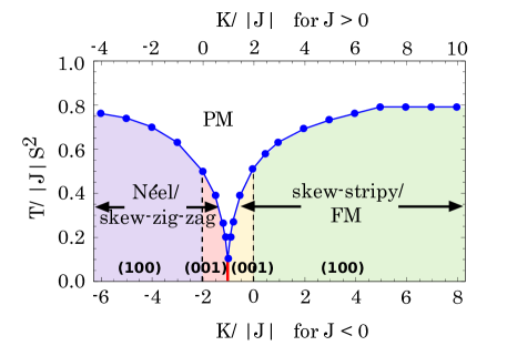
Figure 2: (color online) Finite temperature phase diagram of classical HK model obtained within MC simulation. For both cases of FM $J$ ($J<0$, lower horizontal axis) and AF $J$ ($J>0$, upper horizontal axis), there are two magnetic orders : FM and skew zig-zag phase for FM $J$, Néel and skew-stripy phase for AF $J$. Blue line represents magnetic ordering temperature and red solid line is the phase boundary where the two distinct phases are degenerate. Two black dotted lines are for the exact solvable (anti)-ferromagnetic Heisenberg model. Thermal ObD favors collinear FM / skew zig-zag phase (or Néel / skew-stripy phase) with spins pointing along (001) direction, when $J$ and $-K$ have opposite signs (i.e. frustrated case) in both unrotated and rotated basis. Otherwise, ordered phases have collinear spin states with spins pointing along (100) direction. The errors in the calculated ordering temperatures are smaller than the size of indicated data points.

III.2 Linear spin wave theory

Figure 3: (color online) Finite temperature phase diagram obtained within the Holstein-Primakoff linear spin-wave approximation with $S=1/2$. The top and bottom horizontal axes are for the antiferromagnetic $(J>0)$ and ferromagnetic $(J<0)$ Heisenberg exchanges respectively. These two axes are related by a four-sublattices rotation (see Sec. II). The Néel and skew-stripy labeling of the left and right regions apply to the top axis $(J>0)$ while zig-zag and ferromagnet (FM) apply to the bottom axis $(J<0)$. The first-order phase boundary between these regions is indicated by a solid vertical line. Phase boundaries between different states selected by thermal ObD within each region are indicated by dashed lines. The first-order phase boundary between the thermal ObD-selected and quantum ObD-selected states appears in the lower right of the phase diagram. The estimated ordering temperature is given by the curve between the paramagnetic (PM) region and the magnetically ordered regions. See main text for details on the ObD mechanism and the nature of the selected states.

Competition between thermal and quantum order-by-disorder

Thermal order-by-disorder selects states within the classically degenerate ground state manifold that have the largest thermal fluctuations: an entropic effect. In contrast, quantum order-by-disorder selects states with largest quantum fluctuations and occurs at sufficiently low temperatures when entropic effects are negligible. Since the selection criteria are different between these two mechanisms, the states that are preferred by each can also differ. If the selected ground states do differ and are described by different order parameters, a first-order phase transition is expected at finite temperature. To investigate such a possibility, we analyze the quantum and thermal spin fluctuations at zero and finite temperature about the classical ground state via Holstein-Primakoff linear spin-wave theory. As we will see, the results of this section will also complement those obtained in our classical Monte Carlo simulations (see Sec.III.1).

Parameterizing the classical degeneracy by $\vec{n}$ (see Sec.II), the $\vec{n}$-dependent contribution to the free energy can be written as

$$\delta F(\vec{n},T)=T\sum_{\boldsymbol{k}}\log\left(1-e^{-\omega_{\boldsymbol{k}}(\vec{n})/T}\right)+\frac{1}{2}\sum_{\boldsymbol{k}}\omega_{\boldsymbol{k}}(\vec{n}),$$ (2)

where $T$ is temperature and $\omega_{\boldsymbol{k}}(\vec{n})$ is the linear spin-wave spectrum that is dependent on $\vec{n}$ (the band index has been suppressed). In computing the linear spin-wave dispersion, magnon-magnon interactions have been ignored and only quadratic terms have been retained. We have also taken $S=1/2$ to represent the $j_{\text{eff}}=1/2$ pseudospins of $\beta\text{-}\text{Li}_{2}\text{Ir}\text{O}_{3}$ in the strong-coupling limit.

By minimizing the free energy in respect to $\vec{n}$ at both zero and finite temperatures, we can examine the interplay of quantum ObD and thermal ObD. In Eq.(2), the first term is the free energy of the thermal fluctuations while the last term is the zero-point quantum fluctuation energy correction to the classical energy. Competition between thermal ObD and quantum ObD can occur if the second and last terms possess different global minima in the ground state manifold. A first-order transition will be present if these minima do not possess symmetry-related order parameters. For concreteness, let us now explore this possibility in the Néel and skew-stripy region of the phase diagram—the results for the skew-zig-zag and ferromagnetic regions can be obtained via the four-sublattices rotation introduced earlier (the phase diagram in Fig.3 shows $K/|J|$ axes for both $J>0$ and $J<0$).

Néel $(J>0,K/|J|<1)$:

Both quantum ObD and thermal ObD select the same state for a given $K/|J|$. The $x$-Néel is selected for $K/|J|<0$ while the $z$-Néel is selected for $0<K/|J|<1$. This is shown in Fig.3. Both the selected states and the phase boundary at $K/|J|=0$ match those obtained via our classical Monte Carlo simulations. We note that at the pure antiferromagnetic Heisenberg point, SU(2) symmetry is restored and the accidental degeneracy of the ground state manifold becomes exact hence no ObD is present.

Skew-stripy $(J>0,K/|J|>1)$:

When $1<K/|J|<2$, both quantum ObD and thermal ObD select the $z$-skew-stripy phase, which is in agreement with our classical Monte Carlo results. On the other hand, for $2<K/|J|\lesssim 8.3$, quantum ObD selects the $z$-skew-stripy phase, but thermal fluctuations prefer the $x$-skew-stripy phase. At temperatures of the order $T\approx 0.03~{}J$, a first-order phase transition between these two skew-stripy phases is present, as seen in Fig.3. At $T\gtrsim 0.03~{}J$, the states selected by thermal ObD as well as the phase boundary at $K/|J|=2$ match the results of our classical Monte Carlo results. We again note that the $K/|J|=2$ point is the pure ferromagnetic Heisenberg point in the rotated basis, hence SU(2) symmetry is restored and no ObD mechanism is present.

Ordering temperature

Using linear spin-wave theory, we can also estimate the magnetic ordering temperatures and compare the results with those estimated from our Monte Carlo simulations. We define the ordering temperature as the temperature at which the order parameter (local magnetization) vanishes. Despite the breakdown of linear spin-wave theory when fluctuations are large, this definition would serve as a rough upper-bound of the critical temperature between the ordered phase and the paramagnetic phase. Due to the four-sublattices rotation, this estimate of the ordering temperature applies equally to both antiferromagnetic ($J>0$) and ferromagnetic ($J<0$) Heisenberg exchanges. In Fig.3, the calculated ordering temperatures as a function of $K/|J|$ is shown. We remark that we cannot make a quantitative comparison between the ordering temperature found within classical Monte Carlo and within this spin-wave calculation (the former method considers rigid spins of length $|S|=1$ and incorporates nonlinear interactions while the latter describes quantum mechanical spins with $S=1/2$ within linear spin wave approximation), the general trend of decreasing ordering temperature near the phase boundary between the skew-stripy and Néel region at $K/|J|=1$ is consistent between the two calculations (likewise for the phase boundary between the FM and skew-zig-zag region at $K/|J|=-1$). Linear spin-wave theory estimates that the ordering temperature approaches zero as $K/|J|$ approaches this phase boundary. However, the computed fluctuations in the local magnetization becomes comparable to the local magnetization itself, signaling the breakdown of linear spin-wave theory, hence the estimated ordering temperature may be significantly modified by magnon interactions at this phase boundary.

IV Magnetic field response

The magnetic field response will be useful to clarify the nature of the magnetic order in real materials since the response depends sensitively on the ordering of the spins. In this section, we study the magnetic field response based on both MC simulation in Sec.IV.1 and a semi-classical analysis in Sec.IV.2. Except for the FM case where the field effect is trivial, we estimate the saturation field and its directional dependence in each phase. For the skew-stripy and skew-zig-zag phases, the spin-flop transition is present for general field directions. This originates from the fact that the general skew-stripy and skew-zig-zag phases are neither collinear nor coplanar. For future experiments, we also compute the angle-averaged saturation field on each ordered phase.

IV.1 Classical Monte Carlo

Simple analysis for the saturation field has already been reported in Ref.Lee et al., 2013. Here, we extend that study by investigating the directional dependence of the magnetic field response on each phase at finite temperature using MC simulation. Including magnetic field $\boldsymbol{h}$, the Heisenberg-Kitaev model can be written as

$${H}_{\boldsymbol{h}}=J\sum_{\langle ij\rangle}\boldsymbol{S}_{i}\cdot\boldsymbol{S}_{j}-K\sum_{\langle ij\rangle,\alpha-\rm{links}}S_{i}^{\alpha}S_{j}^{\alpha}-\sum_{i}\boldsymbol{h}\cdot\boldsymbol{S}_{i}.$$

(3)

Here, the magnetic field $\boldsymbol{h}$ includes the Landè $g$-factor. Thus, for a given spin magnitude $S$, the magnetic field is scaled as $g/S$. Unlike our zero-field results, we will need to examine the saturation field of each magnetic phase separately since the four-subalttices rotation transforms a uniform field in the unrotated basis to a site-dependent field in the rotated basis. We also note that, in principle, the (001)- and (100)- states within the same phases show different magnetic field response when the field strength is comparable to the free energy difference between those two states ($\Delta{F}/T\sim 10^{-4}$). However, when the field strength is substantially larger than the free energy difference, the magnetic field response of these two phases will be indistinguishable.

Néel phase:

When the magnetic field is applied in the Néel phase, the uniform magnetization is developed along the field direction, having the Néel order on its basal plane. This results in spin canting and the energy in terms of canted spin angle $\theta$ out of Néel phase is

$$E_{\boldsymbol{h}}^{\text{N\'{e}el}}=(\frac{3J}{2}-\frac{K}{2})(\sin^{2}{\theta}-\cos^{2}{\theta})-h\sin{\theta},$$ (4)

The saturation field is $h_{\rm{sat}}=6J-2K$ where the canting angle $\theta$ becomes $\pi/2$.

Skew-stripy phase:

When the magnetic field is applied perpendicular to the spin directions of either the $(001)$- or the $(100)$-skew-stripy phases, the uniform magnetization is developed along the field direction, resulting in spin canting similar to the Néel phase. The energy in terms of canted spin angle $\theta$ out of skew-stripy phase is

$$E_{\boldsymbol{h}=h(100)}^{\rm{stripy}}=\frac{J}{2}(3\sin^{2}{\theta}-\cos^{2}{\theta})-\frac{K}{2}-h\sin{\theta}.$$ (5)

In this case, the saturation field is $h_{\rm{sat}}^{(100)}=4J$ which is independent of Kitaev interaction $K$. On the other hand, when the magnetic field direction is not perpendicular to the direction of the spin order in the skew-stripy phase, say $\boldsymbol{h}=h/\sqrt{3}(111)$, there is no way to develop uniform magnetization along the field direction and have skew-stripy phase on its perpendicular plane. In principle, the skew-stripy phase belongs to neither collinear nor coplanar spin order except for special cases like $(001)$-,$(100)$-skew-stripy phases where both cases have collinear spin order. Therefore, the skew-stripy phase cannot be established perpendicular to the field direction in general. For a small field, (001)-,(100)-skew-stripy phase is still robust and the system develops uniform magnetization perpendicular to its direction. In the presence of a large magnetic field, however, the Zeeman energy overcomes the spin exchange energy and the skew-stripy phase is eventually destroyed and all spins are polarized along the field direction. Fig.4 shows the magnetization as a function of magnitudes $h$ for $\boldsymbol{h}=h/\sqrt{3}(111)$ at $K/J=4$ and $J>0$. Red, purple and blue points are MC results (lines are drawn as a guide to the eye) for finite temperatures $T/J=0.05,0.1$ and $0.5$ respectively. Black line is the magnetization curve obtained from energy minimization of $H_{\boldsymbol{h}}$ for zero temperature $T/J=0$. As we expected, the (100)-skew-stripy phase is still present and uniform magnetization is developed perpendicular to the (100) direction for a small field $h<h_{\rm{sat}}$. At the saturation field $h_{\rm{sat}}/J\approx 2.7$, the spins are suddenly all polarized along the field direction, resulting in a magnetization jump. Such a magnetization jump corresponds to the spin-flop transition from (100)-skew-stripy phase to fully polarized spin orders along the field direction $\boldsymbol{h}//(111)$. Fig.5 shows the saturation field $h_{\rm{sat}}/J$ for three different cases as a function of $K/J$ in the skew-stripy phase. Black line is the saturation field when the field is applied along (100) direction. As discussed before, the saturation field is $h_{\rm{sat}}^{(100)}=4J$, which is independent of the Kitaev interaction $K$. Blue line is the saturation field $h_{\rm{sat}}^{(111)}$ when the field direction is along (111), obtained by the energy minimization of $H_{\boldsymbol{h}}$ in Eq.(3). In this case, since the skew-stripy phase is stabilized by the interplay between AF Heisenberg interaction ($J>0$) and FM Kitaev interaction ($K>0$), $h_{\rm{sat}}^{(111)}/J$ varies near the phase boundary $K/J=1$ but eventually saturates for large $K/J$ to $h_{\rm{sat}}/J\approx 2.6$. Red line is the angle-averaged saturation field $h_{\rm{sat}}^{\rm{ave}}/J$, obtained by the linear spin-wave calculation. (See Section.IV.2)

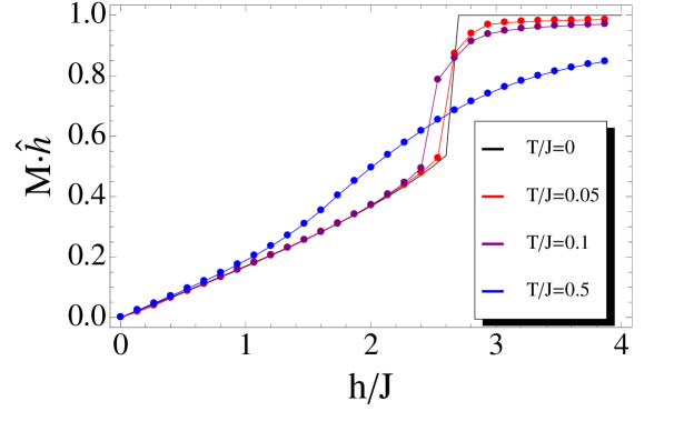
Figure 4: (color online) Magnetization curve as a function of $h/J$ for $\boldsymbol{h}=h/\sqrt{3}(111)$, $K/J=4$ and $J>0$ (in (100)-skew-stripy phase). Red, purple, blue points are MC results for $T/J=0.05,0.1,0.5$ (lines are drawn as a guide to the eye) and black line is from numerical energy minimization of $H_{\boldsymbol{h}}$ for $T/J=0$. The spin-flop transition is present at the saturation field $h_{\rm{sat}}/J\approx 2.7$.

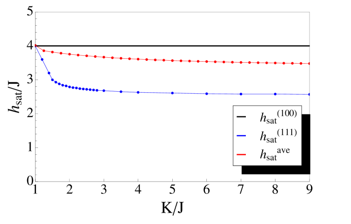
Figure 5: (color online) Plot of saturation field $h_{\rm{sat}}/J$ at zero temperature as a function of $K/J$ within the skew-stripy phase. Black and blue lines are the saturation field when the field is applied in the (100), (111) directions respectively, based on the energy minimization of $H_{\boldsymbol{h}}$ at indicated points. Red line is the angle averaged saturation field obtained by the linear spin-wave calculation.

skew-zig-zag phase:

In the skew-zig-zag phase, AF Kitaev interaction competes with Zeeman energy unlike the case for the skew-stripy phase and the saturation field does depend on both Heisenberg and Kitaev interactions even when the field is applied perpendicular to the collinear spin order. For the field perpendicular to the spin order in (001)-,(100)-zig-zag phase, the energy in terms of canted spin angle $\theta$ out of skew-zig-zag phase is

$$E_{\boldsymbol{h}=h(100)}^{\rm{zig-zag}}=(\frac{J}{2}+\frac{K}{2})\cos^{2}{\theta}+(\frac{3J}{2}-\frac{K}{2})\sin^{2}{\theta}-h\sin{\theta}.$$ (6)

This leads the saturation field to be $h_{\rm{sat}}=2J-2K$ for the field perpendicular to the spin order in (001)-,(100)-zig-zag phase. Similar to the case of the skew-stripy phase, the skew-zig-zag phase does not belong to either collinear or coplanar spin order in general. Hence, for general directions of magnetic field, one can expect a similar magnetization jump like the case of the skew-stripy phase. Fig.6 shows the magnetization as a function of magnetic field $h/J$ for $\boldsymbol{h}=h/\sqrt{3}(111)$ at $K/|J|=-4$ and $J<0$. The spin-flop transition is present at $h_{\rm{sat}}/J\approx 4.3$. For $h<h_{\rm{sat}}$ , the uniform magnetization is linearly increasing with increase of magnetic field $h$. We note that the eight sublattices magnetic order is stabilized to minimize both AF Kitaev spin interaction and Zeeman energy. Fig.7 represents the saturation field for three different cases as a function of $K/|J|$ within the skew-zig-zag phase. Black line is for the saturation field when the field is along (100) direction, $h_{\rm{sat}}^{(100)}=2J-2K$. Blue line is for the saturation field applied in the (111) direction, obtained by energy minimization of $H_{\boldsymbol{h}}$ in Eq.(3). Red line is for the angle-averaged saturation field, $h_{\rm{sat}}^{\rm{ave}}$, obtained by linear spin-wave calculation. (See Section.IV.2) Unlike the skew-stripy phase, the saturation field $h_{\rm{sat}}/J$ increases as a function of $|K/J|$.

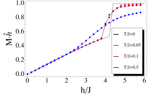
Figure 6: (color online) Magnetization curve as a function of $h/J$ for $\boldsymbol{h}=h/\sqrt{3}(111)$, $K/|J|=-4$ and $J<0$ (in (100)-skew-zig-zag phase). Red, purple, blue points are MC results (lines are drawn as a guide to the eye) and black line is from numerical energy minimization of $H_{\boldsymbol{h}}$ for $T/J=0$. The spin-flop transition is present at the saturation field $h_{\rm{sat}}/J\approx 4.3$.

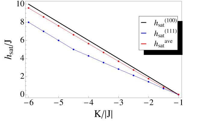
Figure 7: (color online) Plot of saturation field $h_{\rm{sat}}/J$ at zero temperature as a function of $K/|J|$ within the skew-zig-zag phase. Black and blue lines are the saturation field when the field is applied to (100), (111) directions respectively, based on the energy minimization of $H_{\boldsymbol{h}}$ at indicated points. Red line is the angle averaged saturation field obtained by linear spin-wave calculation.

IV.2 Linear spin wave theory

The saturation field at zero temperature can also be computed within linear spin-wave theory. By applying a sufficiently large field, the classical ground state is ferromagnetically ordered in the direction of the magnetic field. We then consider the spin-wave spectrum about such an ordered state and lower the magnetic field strength until the spin-wave spectrum becomes gapless. Further decrease in the applied-field strength will render the classical ferromagnetic state unstable, indicating that the saturation field has been reached.

Although the magnetization curve and spin-flop transitions revealed in the previous section could not be obtained within this approach, linear spin-wave theory allows us to efficiently compute $h_{\text{sat}}$ with arbitrary field directions and perform angle-averages, which are of particular experimental interest for single-crystal, polycrystalline, and powder samples.

Similar to Sec.IV.1, we set the spin magnitude $S$ and Landè g-factor to be arbitrary: the magnetic field is in units of $g/S$.

\begin{overpic}[scale={.1}]{figs/hsat_direction.png} \put(10.0,305.0){a)} \put(132.0,305.0){b)} \put(10.0,173.0){c)} \put(132.0,173.0){d)} \put(90.0,5.0){$h_{\text{sat}}/\max(h_{\text{sat}})$} \end{overpic}

Figure 8: (color online) Field-direction dependence of saturation field ($h_{\text{sat}}$). The color maps indicate the fraction of the saturation field compared to the maximum attained in directions perpendicular to the cubic axes. Red contours are shown indicating $h_{\text{sat}}/\max(h_{\text{sat}})$ values of 0.9 and 0.8. Figures a) and b) are for the skew-stripy phase at $K=1.5|J|$ and $K=3.0|J|$ respectively. Notice the solid angle with low saturation field grows as $|K|$ increases. Figures c) and d) are for the skew-zig-zag phase at $K=-2.0|J|$ and $K=-4.0|J|$. Notice the opposite trend: the solid angle with low saturation field decreases as $|K|$ increases.

Néel ($J>0,K/|J|<1$):

All the Néel states within the ground state manifold are collinear, hence no spin-flop transition is expected at field strengths larger than the quantum zero-point energy splitting (which is smaller than $10^{-3}|J|$). This also implies that the saturation field does not depend on the applied direction. The angle-averaged saturation field found is exactly $h^{\text{ave}}_{\text{sat}}=6J-2K$, which agrees with the expression obtained from Eq.(4).

Skew-stripy ($J>0,K/|J|>1$):

For fields applied perpendicular to the collinear skew-stripy order, $h_{\text{sat}}=h^{(100)}_{\text{sat}}=4~{}J$ is independent of $K/|J|$. In Fig.8a) and 8b), we also see that the saturation field is sensitive to the field direction due to the spin-flop transition and it is reduced when the field is applied in the $\langle 111\rangle$-direction with $h_{\text{sat}}\approx 0.75h^{(100)}_{\text{sat}}=3~{}J$. The $K/|J|$ dependence is manifested in the solid angle where the saturation field is reduced: Fig.8a) ($K/|J|=1.5$) has a smaller solid angle with reduced $h_{\text{sat}}$ compared to Fig.8b) ($K/|J|=3.0$). This implies that the angle-averaged saturation field will decrease as $K/|J|$ increases, which can be seen in Fig.5 ($h^{\text{ave}}_{\text{sat}}$ approaches $3.4~{}J$ with increasing $K/|J|$). We also note that the $h^{\text{ave}}_{\text{sat}}$ is largely independent of $K/|J|$.

Skew-zig-zag ($J<0,K/|J|<-1$):

The saturation field of the skew-zig-zag phase also possesses directional dependence due to the general non-coplanar nature of the skew-zig-zag phase that causes the spin-flop jump in magnetization. This is readily seen in Fig. 8c and Fig.8d. Contrasting with the skew-stripy phase, as $|K/J|$ increases, the region with reduced saturation field decreases in size. This can be seen by comparing Fig.8c ($K/|J|=-2.0$) with Fig.8d ($K/|J|=-4.0$). The angle-averaged saturation field is shown in Fig.7 and is below the value of $h^{(100)}_{\text{sat}}=2(J-K)$ due to the reduction in $h_{\text{sat}}$ for general field directions. As $|K/J|$ increases, $h^{\text{ave}}_{\text{sat}}$ approaches $h^{(100)}_{\text{sat}}$.

Magnetic order	Parameter region	$\Theta_{\rm{CW}}/h^{\text{ave}}_{\text{sat}}$
Néel	$J>0,K/|J|<1$	$-1/2$
Skew-stripy	$J>0,K/|J|>1$	$(K/J-3)/4$
Skew-zig-zag	$J<0,K/|J|<-1$	$(K-3J)/(2J-2K)$

Table 1: Table of the ratio of Curie-Weiss temperature $\Theta_{\rm{CW}}$ to angle-averaged saturation field $h^{\text{ave}}_{\text{sat}}$ as estimated from linear spin-wave theory. The saturation field $h^{\text{ave}}_{\text{sat}}$ is scaled by $g/S=4$. For the skew-stripy and skew-zig-zag phases, the quoted result of $\Theta_{\rm{CW}}/h_{\rm{sat}}^{\rm{ave}}$ is for fields along (100), however, this is a good approximation to the angle-averaged result (which is slightly smaller in magnitude).

V Discussion and Summary

Related to future experiments on the material, we suggest estimating the magnitudes of the Heisenberg and Kitaev interactions $J,K$ based on our theory. From experiments, one can measure the Curie-Weiss temperature $\Theta_{\rm{CW}}$, ordering temperature $T_{c}$, and saturation field $h_{\rm{sat}}$. In the high temperature limit, the Curie-Weiss temperature is given by $\Theta_{\rm{CW}}=(K-3J)/4$ (for $S=1/2$). Since we obtained an estimation of the saturation field and the ordering temperature from MC simulation for each magnetic phase, we can estimate the actual values of $J$ and $K$ based on these three parameters and speculate which ordered phase is realized in the real material. Table.1 shows the ratio of Curie-Weiss temperature $\Theta_{\rm{CW}}$ to angle-averaged saturation field $h_{\rm{sat}}^{\rm{ave}}$ for different ordered states (details are discussed in Sec.IV). From the observation of the saturation fields listed in Table.1, one can point out that in the Néel and skew-zig-zag phase, the system can have small $h_{\rm{sat}}^{\rm{ave}}$ even when exchange interactions $J$ and $K$ are large, due to the cancellation between them. On the other hand, if the system is in the skew-stripy phase, the saturation field can serve as an estimation of $J$.

In summary, we studied the finite temperature phase diagram of the Heisenberg-Kitaev (HK) model on a 3D hyperhoneycomb lattice. Based on classical MC simulation and a semi-classical analysis using Holstein-Primakoff bosons, we investigated the magnetic ordering temperatures and ObD effects in the HK model. Unlike the case for the 2D HK model on the honeycomb lattice, the ordering temperature is finite even in the limit of the pure (anti-) ferromagnetic Heisenberg points $K/|J|=0$ and their equivalent points $K/|J|=\pm 2$ for $\pm J>0$ after the four-sublattice rotation. In addition, the overall energy scale of ordering temperatures in the HK model on the 3D hyperhoneycomb lattice is higher than the ones on the 2D honeycomb lattice as expected.Price and Perkins (2013) Based on the MC simulation, one can see that the ordering temperature is largely suppressed at the transition point $K/|J|=\pm 1$ for $\pm J>0$ due to the magnetic frustration. Away from the transition point, however, the ordering temperature $T/|J|$ increases with increase of $K/|J|$. Linear spin-wave theory also shows the same trend of ordering temperature and it reasonably estimates the ordering temperature compare to the MC simulation. We also studied ObD effects from both thermal and quantum fluctuations. These two different types of fluctuations compete with each other and they favor different magnetic orders in a certain parameter region. Just below the ordering temperature, the entropy effect is large and the states selected by thermal ObD are favored. At very low temperatures, however, zero-point quantum fluctuations are dominant and the states selected by quantum ObD are favored. Such competition between thermal ObD and quantum ObD results in an additional phase transition below the ordering temperature. Finally, we investigated the magnetization process and the saturation field as a function of $J$ and $K$ for each phase. For general field direction, we found that the spin-flop transition is present in both skew-stripy phase and skew-zig-zag phase. Such spin-flop transitions originate from the non-coplanar character of the general skew-stripy/skew-zig-zag spin order. For comparison with future experiments, we have also investigated in detail the directional dependence of the saturation field and calculated the angle-averaged saturation field at zero-temperature.

VI Appendix

VI.1 Free energy calculation

In this Appendix, we discuss the free energy calculation in the ferromagnetic phase for $K/|J|>1$ and $J<0$ and find the state selected by thermal ObD. Let us start from a ferromagnetic ground state and expand fluctuations by writing

$$\boldsymbol{S}_{i} = \boldsymbol{\bar{S}}\sqrt{1-\Pi_{i}^{2}}+\boldsymbol{\Pi}_{i}~{},$$ (7)

$$\boldsymbol{\Pi}_{i} = \boldsymbol{v}_{1}\phi_{i}+\boldsymbol{v}_{2}\chi_{i}~{},$$ (8)

where $\boldsymbol{\bar{S}}$ is FM order pointing along certain direction and $\boldsymbol{\Pi}_{i}$ is lying on its basal plane satisfying $\boldsymbol{\bar{S}}\cdot\boldsymbol{\Pi}_{i}=0$. This automatically satisfies a constraint $|\boldsymbol{S}_{i}|=1$ and the partition function becomes

$$\mathcal{Z} = \int\mathcal{D}\boldsymbol{S}~{}e^{-\beta H}=\int\mathcal{D}\chi\mathcal{D}\phi~{}e^{-\mathcal{S}}~{},$$ (9)

$$\mathcal{S} = \frac{1}{2T}\sum_{ij}~{}(\phi_{i}\tilde{J}_{ij}\phi_{j}+\chi_{i}\tilde{J}_{ij}\chi_{j}+\phi_{i}{P}_{ij}\phi_{j}+\chi_{i}{Q}_{ij}\chi_{j}+2\phi_{i}R_{ij}\chi_{j})$$ (13)

$$= \frac{1}{2T}\sum_{\boldsymbol{k}}~{}\left(\begin{array}[]{cc}\phi_{\boldsymbol{k}}^{*}&\chi_{\boldsymbol{k}}^{*}\end{array}\right)M_{\boldsymbol{k}}\left(\begin{array}[]{cc}\phi_{\boldsymbol{k}}\\ \chi_{\boldsymbol{k}}{}\end{array}\right)~{},$$

where

$$\tilde{J}_{ij} = J_{ij}-3J\delta_{ij},$$

$$P_{ij} = -K_{ij}^{\alpha}(v_{1}^{\alpha})^{2}+K\delta_{ij},$$

$$Q_{ij} = -K_{ij}^{\alpha}(v_{2}^{\alpha})^{2}+K\delta_{ij},$$

$$R_{ij} = -K_{ij}^{\alpha}(v_{1}^{\alpha}v_{2}^{\alpha}).$$ (14)

Here, we keep only quadratic terms of $\chi$ and $\phi$ assuming that this Gaussian action well behaves at low enough temperature. The free energy $\mathcal{F}$ can be represented as

$$F = -T~{}{\rm{ln}}~{}(\mathcal{Z})$$ (15)

$$= \frac{T}{2}\sum_{\boldsymbol{k},a}~{}{\rm{ln}}~{}(W_{a}(\boldsymbol{k})/2\pi T),$$

where $W_{a}(\boldsymbol{k})$ is the $a$-th eigenvalues of matrix $M_{\boldsymbol{k}}$ defined in Eq.(13), at a given wave vector $\boldsymbol{k}$. The connection between this classical approach and a semi-classical analysis using Holstein-Primakoff bosons, can be understood in the following way. In high temperature limit, Eq.(2) (in the main text) can be rewritten as

$$F(T) = T\sum_{\boldsymbol{k},\omega_{\boldsymbol{k}}>0}{\rm{ln}}(1-e^{-\omega_{\boldsymbol{k}}/T})$$ (16)

$$\approx T\sum_{\boldsymbol{k},\omega_{\boldsymbol{k}}>0}{\rm{ln}}~{}\frac{\omega_{\boldsymbol{k}}}{T}.$$

The trace of ${\rm{ln}}~{}\omega_{\boldsymbol{k}}$ is consistent with trace of $1/2~{}{\rm{ln}}~{}W_{a}(\boldsymbol{k})$ in Eq.(13) and in this way, the free energy of semi-classical analysis recovers the free energy of classical approach in high temperature limit.

Fig.9 shows the calculated free energy for different FM order with spins along $\ (001),(100),(110),(111)$ at $T/|J|=1$. The free energies of magnetic orders along $(001)$ or $(100)$ are always lower than the others for entire parameter regime of $K/|J|$ within FM order, resulting in either $(001)$- or $(100)$-FM states being selected by thermal fluctuations. The free energy difference between those two states are quite small, so we plot the energy difference $\Delta F/T=(F_{\boldsymbol{\bar{S}}={(001)}}-F_{\boldsymbol{\bar{S}}={(100)}})/T$ in Fig.10. As can be seen in Fig.10, the free energy difference $\Delta F/T$ changes its sign with the sign of Kitaev term $K$. For $K/|J|>0$ where both Heisenberg and Kitaev interactions favor the FM order (unfrustrated case), thermal ObD selects the $(100)$-FM order. On the other hand, for $K/|J|<0$ where Heisenberg and Kitaev interactions are frustrated, thermal ObD favors the $(001)$-FM order. We also found that such thermal ObD effect exists in the Néel order. For unfrustrated case (both $J$ and $K$ have same sign), thermal fluctuation favors the Néel order with spins pointing along $(100)$, whereas, it favors the Néel order along $(001)$ for frustrated case (when $J$ and $K$ have different signs). As emphasized in Sec.II, the FM order for $J<0$ can be directly mapped onto the skew-stripy order for $J>0$, similarly the Néel order for $J>0$ onto the skew-zig-zag order for $J<0$, followed by a four-sublattices rotation introduced in Sec.II. Hence, one can expect the same thermal ObD effect for both skew-stripy phase and skew-zig-zag phase.

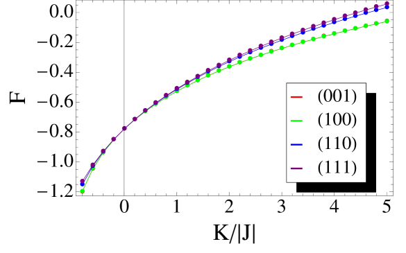
Figure 9: Calculated free energy from the quadratic order of fluctuating fields $\phi,\chi$ for different FM ordering vectors : Red, green, blue and purple colored lines are free energies for FM order $\boldsymbol{\bar{S}}//(001),(100),(110),(111)$ respectively. Free energy differences between $\boldsymbol{\bar{S}}=(001)$ and $\boldsymbol{\bar{S}}=(100)$ are replotted in Fig.10 for a better resolution.

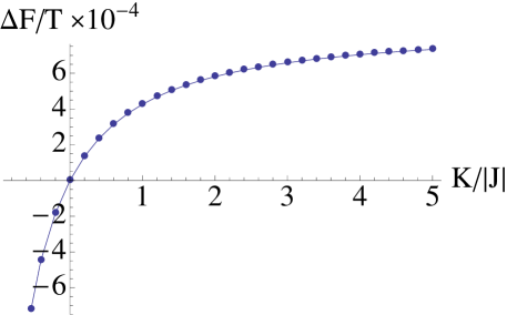
Figure 10: Plot of free energy difference between the two different FM order, $\Delta F/T=(F_{\boldsymbol{\bar{S}}={(001)}}-F_{\boldsymbol{\bar{S}}={(100)}})/T$. Thermal ObD selects FM order along $(001)$ for $K/|J|<0$, whereas, it favors FM order along $(100)$ for $K/|J|>0$.