Free volume distribution of nearly jammed hard sphere packings

Abstract

We calculate the free volume distributions of nearly jammed packings of monodisperse and bidisperse hard sphere configurations. These distributions differ qualitatively from those of the fluid, displaying a power law tail at large free volumes, which constitutes a distinct signature of nearly jammed configurations, persisting for moderate degrees of decompression. We reproduce and explain the observed distribution by considering the pair correlation function within the first coordination shell for jammed hard sphere configurations. We analyze features of the equation of state near jamming, and discuss the significance of observed asphericities of the free volumes to the equation of state.

Disordered, structurally arrested forms of matter arise through a variety of procesess, such as the glass transition in dense, cold liquids, gelation, jamming in granular matter, to name a few examplesdebenedetti-book ; binder-kob-book ; heterogeneity-book ; torquato-book . The nature of these processes and their interrelation are topics of considerable current research activity. Much of the interest is focussed on understanding the manner in which the relaxation dynamics and transport properties change in the fluid state upon approaching the arrest transition. Temperature, density and applied stress are involved as control parameters that determine the transition from an arrested to a fluid state in different systems, and a unified jamming phase diagram has been discussed as a possible description of the arrested-to-fluid transition liu . Recent theoretical work, however, draws a distinction between the glass and jamming transitions (summarized, e. g. in parisi-zamponi-review ), and the exact relationship between these transitions is a topic of ongoing research.

Considerable work addressing the nature of the jamming transition has focussed on packings of hard spheres, dating back to the seminal work of Bernal and co-workers bernal ; bernalmason , who identified a random close packing (RCP) of spheres with a packing fraction of $64\%$, attained as the maximum density for amorphous packings of equal sized spheres (we express density values in packing fractions throughout). Considering the hard sphere fluid as the initial, thermodynamic equilibrium state from which jammed configurations are generated, RCP would represent a limit state at which the pressure would diverge. While such a point would correspond to a state of structural arrest, many studies suggest that a glass transition precedes jamming, at finite pressure speedyjeos ; speedyhsgt ; krzakala ; parisi-zamponi ; parisi-zamponi-review . Further, in analogy with the glass transition, it has been suggested and demonstrated that the jamming transition too does not occur at a unique point but can occur over a range of densities speedyhsgt ; krzakala ; chaudhuri ; sal1 .

In addition to such analyses concerned with thermodynamic and dynamic (or kinetic) aspects, much attention has been focussed on geometric features of jammed configurations mrj ; torquatorev ; donev ; epitome ; silbert ; bruic ; wyart ; sal2 ; ogarko (in contrast to the relatively scant attention to structure in the context of glass formation). From such a geometric point of view, the proposal of a unique random close packing has been questioned mrj , and it has been proposed that a more suitable notion is that of maximally random jammed packings. Although the jamming density itself is not unique, interestingly, many geometric features remain robust chaudhuri . An important example is the power law singularity in the pair correlation function near contact, observed in addition to the delta function at contact epitome ; silbert ; donev ; wyart ; charbonneau . The origins and consquences of these unique geometric features are of considerable current interest.

One of the important ways of characterizing the geometry of hard sphere packings is the distribution of free volumes sastryfreevol ; maiti . The free volume, defined as the volume available to the centre of a hard sphere while all other spheres remain fixed, is further directly related to the equation of state (EOS) speedyhs ,

$${P\over\rho k_{B}T}=1+{\sigma\over 2D}\left<{s_{f}\over v_{f}}\right>,$$ (1)

where $P$ is the pressure, $T$ is the temperature, $\sigma$ the diameter of the spheres, $D$ is the spatial dimensionality ($D=3$ for all the results shown in this work.), $v_{f}$ and $s_{f}$ are respectively the free volume and the surface area of the free volume. An exact algorithm for determining the volume and surface area of cavities in polydisperse sphere packings, developed in sastryalgo has been employed sastryfreevol ; maiti to study free volume distributions in (monodisperse and bidisperse) hard sphere fluids.

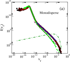
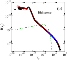
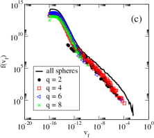
Figure 1: Free volume distributions for (a) monodisperse (circles: $\phi_{init}=0.4487$; squares: $\phi_{init}=0.533$) and (b) (component 1 of the) bidisperse sphere packings ((circles: $\phi_{init}=0.363$; squares: $\phi_{init}=0.5919$) close to the jamming point, for the cases listed in tables I and II. Free volume distributions of both packings have a power law tail of exponent $-0.9$ (solid lines). The distributions are the same regardless of the jamming density. The expected free volume distributions, based on extrapolating (by a polynomial fit to the parameters in Eq. 2 and extrapolating them to the jamming density) those for the fluid (dot dashed lines), are shown for comparison. The distribution obtained without considering the free volumes of rattlers is also shown in (a) for one case ($\phi_{init}=0.4487$) (diamonds), with a power law tail with exponent $-1$) (dashed line). (c) Free volume distributions for monodisperse spheres with selected numbers of contact neighbors, $q=2,4,6,8$, for $\phi_{init}=0.4487$.

A cavity is a connected subset of the void space, which is defined as the volume that lies outside the union of spheres that define the system under consideration. For defining the free volumes, one considers exclusion spheres located at the coordinates of each hard sphere, with radius equal to the radius of the hard sphere plus the radius of the sphere whose free volume one wishes to compute. Given a configuration of $N$ hard spheres, the free volume of a given hard sphere is the volume of the cavity in which its coordinates lie, in a configuration of $N-1$ spherses excluding the sphere under consideration. The algorithm for computing cavity volumes, described in detail in sastryalgo ; maiti , involves the following steps, for the calculation of free volumes in hard sphere configurations: (i) A Voronoi or generalized Voronoi (radical plane) construction. (ii) Identification of cavities based on connected Voronoi vertices that lie in the void space. (iii) Identification of the set of Delaunay tetraheda that enclose a given cavity. (iv) Computation of the cavity volume and surface area of the cavity contained in each Delaunay tetrahedron. An efficient way of implementing this algorithm to the free volume calculation without repeated tessellations is described in sastryfreevol ; maiti .

The free volume distributions, over a wide range of densitiessastryfreevol ; maiti , is described well by the form

$$f(v_{f})\propto v_{f}^{\alpha}\exp(-\beta v_{f}^{\gamma})$$ (2)

where the parameters $\alpha$, $\beta$ and $\gamma$ are smoothly varying functions of density yielding a mean free volume that decreases with density. Strictly at the jamming point, the free volumes must equal zero, if one excludes ’rattlers’, which are spheres with the number of contacts $q\leq 3$, and are therefore free to move in some directions without hindrance from the contact neighbors. However, slightly below the jamming poing, the free volumes are finite, and it is natural to ask what the free volume distributions look like at such densities close to jamming. We address this question in this paper, by generating jammed configurations of monodisperse and bidisperse hard spheres, and calculating the free volume distributions of nearly jammed configurations obtained by decompressing them slightly.

We generate jammed configurations following the procedure in chaudhuri ; berthier , wherein starting from an equilibrated hard sphere fluid at initial density $\phi_{init}$, a fast initial compression is effected using a Monte Carlo simulation till the pressure reaches $10^{3}$ (reduced units are used throughout). The system is next treated as made of soft spheres ohern (with interaction potential $V_{\alpha\beta}=(1-\frac{r_{ij}}{\sigma_{\alpha\beta}})^{2}$ for $r_{ij}\leq\sigma_{\alpha\beta}$; = 0 for $r_{ij}>\sigma_{\alpha\beta}$, where $\alpha$, $\beta$ represent different sizes of spheres $i$, $j$), and compressed further, till the energy per particle is $10^{-5}$. The system is then decompressed in steps, following energy minimization at each step. A jammed configuration (and jamming density $(\phi_{J})$) is identified by the condition that the single particle energy reaches $e=10^{-16}$ or smaller. For data shown in figures 1 and 2, the jammed configurations are generated with a tolerance in packing fraction of $10^{-5}$, and for figures 4 and 5, $10^{-8}$ (based on the decompression steps used). We note that we consider only energy minimum structures throughout this procedure, and dynamical effects that may matter in real systems do not play a role in determining the jammed configurations.

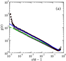
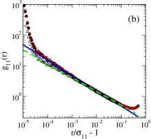
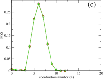
Figure 2: Pair correlation function g(r) for (a) mono and (b) (component 1 of the) bidisperse sphere packings for the cases shown in Fig. 1. Power law fits close to contact are shown, with exponent $-0.45$ for monodisperse packings and $-0.5$ for the bidisperse packings. g(r) calculated excluding rattlers is also shown (open triangles) along with power law fit lines (dashed lines) for comparison. (c) The distribution of the number of contact neighbors for the monodisperse case.

We study monodisperse and bidisperse hard sphere systems of size $N=2000$. The bidisperse system is a 50:50 mixture of spheres of diameter $\sigma$ (component 1) and $1.4\sigma$ (component 2). We choose three initial densities for the monodisperse fluid, which are smaller than the packing fraction ($0.545$) of spontaneous crystallization. Four different initial fluid densities of bidisperse hard spheres are chosen. The jammed densities are evaluated after averaging over $500$ ($100$) independent configurations for figures 1,2 (figures 4,5), ensuring lack of crystallinity through a calculation of orientational order parameters. The statistics of jammed densities for different initial fluid densities are shown in the table I(monodisperse) and table II(bidisperse).

$\phi_{init}$	$\sim\phi_{J}(e\leq 10^{-16})$	Rattlers
0.533	0.6419	$1.6\%$
0.4487	0.6394	$1.7\%$
0.2841	0.6392	$1.7\%$

Table 1: Statistics of jammed configurations of monodisperse spheres for system size $N=2000$. $\phi_{init}$, $\phi_{J}$ are the initial and jammed configuration densities, and $e$ is the energy per particle. Rattlers are spheres with number of contacts $q\leq 3$.

$\phi_{init}$	$\sim\phi_{J}(e\leq 10^{-16})$	Rattlers
0.5919	0.6605	$6.1\%$
0.5704	0.6554	$5.6\%$
0.5396	0.6498	$4.9\%$
0.363	0.6476	$4.6\%$

Table 2: Statistics of jammed configurations of bidisperse spheres for system size $N=2000$. Symbols as in table I.

We calculate the distribution of free volumes, using the algorithm described in sastryfreevol ; maiti , for configurations that are decompressed (by $10^{-8}$ in packing fraction) from the jammed configurations and thermalized by performing a short Monte Carlo simulation of $1000$ attempted random displacements (of magnitude comparable to the distance created between contact neigbhors by the decompression) per sphere. By extrapolating the parameters of Eq. 2, one may expect a very narrow free volume distribution near the jamming point. Fig. 1 shows the free volume distribution near jamming for both the monodisperse and bidisperse packings. In addition to a peak at small free volumes, the distribution displays an unexpected power law tail $(\approx v_{f}^{-{\color[rgb]{0,0,0}\delta}})$, over eight orders of magnitude of free volumes. For both mono- and (both components of the) bidisperse packings, the exponent ${\color[rgb]{0,0,0}\delta}=-0.9$. These distributions, which are very different from the extrapolation from the fluid state, do not depend on the jamming density. We verify that the tail is not due to rattlers. As shown in Fig. 1 (a), eliminating rattlers from consideration alters the exponent in the power law but does not eliminate the feature. We also verify that the Lubachevsky-Stillinger procedurelubachevsky for generating jammed configurations also produces the power law tail. As supported by results discussed below, the observed power law tail is thus a structural signature of nearly jammed particle packings.

Since the free volume of a sphere is determined by the location of its neighbors, the power law tail in the free volume distribution may be related to the pair correlation function $g(r)$, which, in addition to a delta function at contact, has a well-studied singularity near contact, $g(r)\approx(\frac{r}{\sigma}-1)^{-{\color[rgb]{0,0,0}\eta}}$ silbert ; donev ; chaudhuri ; charbonneau ; wyart for jammed configurations. The connection is not straight-forward, since $g(r)$ is a two-body property, whereas the free volume of a sphere is a many-body property that depends on the positions of all its neighbors. Further, it is reasonable to expect, as indeed generally done, that the contact neighbors bound the (compact) free volume of a sphere in slightly decompressed configurations. The possibility that non-contact neighbors may play a role at all is therefore suggested by our surprising finding of a large free volume tail, which we explore. As a preliminary test, we compute the free volume distribution for groups of spheres each of which has a particualr number of contact neighbors (we discuss the distribution of contact numbers further below). These partial distributions are shown in Fig. 1(c), for contact number $q=2,4,6,8$. While for $q=6,8$ the partial distributions are confined to be small free volume peak, for $q=2,4$, one has a substantial contribution in the tail. Thus, the number of contact neighbors plays a crucial role in determining the free volumes, and for contact neighbors less than $6$, the free volumes are significantly distributed in the tail.

In Fig. 2 (a) and (b) we show the $g(r)$, which exhibits a power law regime near contact with exponent value ${\color[rgb]{0,0,0}\eta}=-0.45$ for monodisperse packings and ${\color[rgb]{0,0,0}\eta}=-0.5$ for component 1 of the bidisperse case. As discussed previously silbert ; donev ; charbonneau , and we show in Fig. 2, the $g(r)$ exponent depends whether rattlers are included in its evaluation or not. We analyze configurations which include rattlers, and choose the distance at which $g(r)$ deviates from the power law, $(\approx 10^{-5})$, as the cutoff to identify contact neighbors. The distribution of the number of contact neighbors is shown in Fig.  2(c) for the monodisperse case. Interestingly, roughly a third of the spheres have less than $6$ contact neighbors, and thus the spheres whose free volumes may contribute to the tail of the distribution is not a negligible fraction. We note that the population with $q\leq 3$ (i. e. rattlers) are expected to have $q=0$ with a precise definition of contact neighbors, and indeed find that the population of spheres with $q=1,2,3$ decreases with an increase in the precision with which contact neighbors are identified.

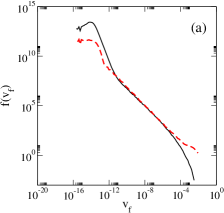
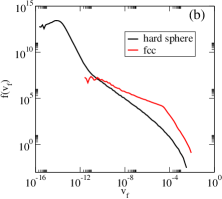
Figure 3: (a) Comparison of the free volume distribution of monodisperse sphere packings (solid line) with the icosahedron model. (dashed line). (b) Comparision of the free volume distribution of monodisperse sphere packings (solid line) with the model calculation wherein the neighbors occupy nearest neighbor positions in the FCC lattice.

We next consider a toy computation wherein the free volume of a sphere in the centre of an icosahedral cluster of spheres is considered. Starting with a regular, compact configuration, the $12$ spheres on the periphery are displaced according to the distribution of neighbor distances observed for monodisperse packings. As shown in Fig. 3 (a), the free volume distribution for the icosahedron model indeed displays a power law tail, with the correct exponent, though it is too simple a model to capture all relevant details accurately, such as the relative amplitudes of the peak and the power law tail. Choosing initial neighbor positions arranged in an $FCC$ configuration, rather than an icosahedron, leads to a distribution with different features and a different exponent for its tail, as shown in Fig. Fig. 3 (b) These observations, suggest that the free volume distribution depends sensitively on the many body correlations of neighbor positions, which needs further analysis to elucidate.

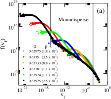
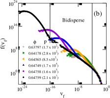
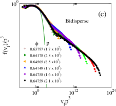
Figure 4: Evolution of the free volume distribution of (a) monodisperse and (b) (component 1 of the) bidisperse sphere packings, upon decompression. Distributions for the bidisperse case have been scaled with $p^{3}$ in (c) ($p={P\over\rho k_{B}T}-1$) to emphasize that invariant shape of the peak of the distributions, which is significantly broader than for the liquid (Eq. 2 and Fig. 1; solid line). The densities $\phi$ and $p$ of (some of) the decompressed configurations are shown in the legends. Vertical lines in panel (a) indicate the range of $v_{f}$ over which one observes the power law tail for the highest density in both the cases.

We next consider the manner in which the free volume distribution evolves upon decompression. To do so, the sizes of the spheres are rescaled to correspond to a range of densties lower than the jamming density, and the configutations are thermalized by performing short Monte Carlo simulations (see above) at each density. As shown in Fig. 4 (a) and (b), the distributions evolve towards those found in the liquid state, but interestingly, the power law tail persists over a finite range of densities.

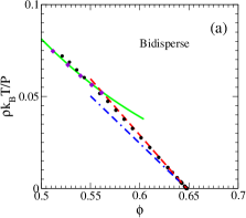
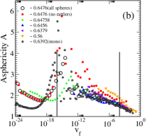
Figure 5: (a) The equation of state (EOS) near jamming of bidisperse system. The solid line represents the Carnahan-Starling (CS) EOS. Also shown (diamonds) are pressures for the fluid obtained from Eq. 1. The data points from decompressed configurations are fit to the form 3 with $C=2.53$ (dashed lines) with an intersection with the CS EOS at $\phi=0.562$. The line with $C=D$ is also shown for reference (dot dashed lines). (b) Asphericity $A$ (see text) shown for bidisperse configurations for a range of densities. Aspericities for the monodisperse case, and the fluid ($\phi=0.56$) are shown for comparison.

We use the configurations generated above to calculate the pressures, using Eq. 1. The EOS near the jamming point predicted by Salsburg and Wood wood , obtained by assuming compact free volumes,

$$\frac{P}{\rho k_{B}T}=\frac{C\phi_{J}}{\phi_{J}-\phi}\mbox{ ; $C=D$}.$$ (3)

This prediction has been verified donev in earlier work but for configurations without rattlers. Speedy speedy1 reported $C=2.67$ for monodisperse hard spheres. As discussed in donev ; charbonneau_2 , the presence of rattlers will reduce the value of $C$ linearly with the fraction of rattlers. However, our results for the bidisperse system, shown in Fig. 5(a), consistent with a value of $C=2.53$, cannot be explained by the presence of rattlers alone (see Table II, $\phi_{init}=0.363$. Rattler fraction $f=4.6\%$ implies $C=D(1-f)=2.862$), and must also have a contribution from free volume heterogeneitydonev ; charbonneau_2 . As can be seen from Fig. 4(c), the peak of the free volume distribution, plotted against free volume scaled by $p^{3}$ (based on $p\sim 1/\delta$, $v_{f}\sim\delta^{3}$ where $\delta$ is the distance to the contact neighbors) has a density invariant shape that is significantly broader than the form obeyed by the liquid. We also calculate the asphericity $A$ of free volumes, defined as $A={1\over 2D}{s_{f}\over v_{f}^{2/3}}$ ($A=0.806$ for spherical and $=1$ for a cubic free volumes). As shown in Fig. 5(b), free volumes over the full range of values show asphericity to varying degrees, for different degrees of decompression, with the asphericities being maximum in the initial part of the power law tail in all cases. The role played by these two factors merits further investigation. It is interesting to note that the intersection of the free volume EOS Eq. 3 with the fluid (CS) EOS occurs around $0.562$, close to the experimental number of $0.58$ for the glass transition as described by mode coupling theory. Since the EOS Eq. 3 is obtained for jammed configurations decompressed with a very short equilibration time, it is interesting to interpret the intersection density of $0.562$ as the limiting density for the glass in the limit of infinitely fast decompression, which has consistency with the emergence of the mode coupling transition as a limit of stability in some descriptions of the glass transition franz . It should be observed that the intersection density would be very much lower if $C=D$. Thus, the presence of rattlers and free volume anisotropies seem to have a role in determining a meaningful transition density from the glass to the fluid states.

In summary, we have calculated free volume distributions for nearly jammed sphere packings, and show that they exhibit a characteristic power law tail, which we show is related to the power law singularity in the pair correlation function. The power law tail persists for moderate degrees of decompression and are thus a signature of packing close to jamming. We show evidence that the deviations of the equation of state close to jamming from the prediction for ideal jammed packings arise from the asphericities of the free volumes in addition to the presence of rattlers.

I Acknowledgements:

We wish to thank Salvatore Torquato, Francesco Zamponi, Giorgio Parisi, Patrick Chabonneu, Gilles Tarjus and Sidney Nagel for useful discussions.

References

- (1) P. G. Debenedetti, Metastable Liquids: Concepts and Principles (Princeton University Press, 1996).
- (2) K. Binder and W. Kob, Glassy Materials and Disordered Solids: An Introduction to their Statistical Mechanics, (World Scientific, 2005).
- (3) Dynamical Heterogeneities in Glasses, Colloids, and Granular Media, L. Berthier, et al., eds. (Oxford University Press, 2011)
- (4) S. Torquato, Random Heterogeneous Materials: Microstructure and Macroscopic Properties Springer-Verlag (2002).
- (5) A. J. Liu and S. R. Nagel, Nature 396, 21 (1998).
- (6) G. Parisi and F. Zamponi, Rev. Mod. Phys. 82, 789 (2010).
- (7) J. D. Bernal, Nature 185, 68 (1960)
- (8) J. D. Bernal and J. Mason, Nature 188, 910 (1960).
- (9) R. J. Speedy, J. Chem. Phys. 100 6684 (1994).
- (10) R. J. Speedy, Mol. Phys. 95 169 (1998).
- (11) F. Krzakala and J. Kurchan, Phys. Rev. E 76, 021122 (2007).
- (12) G. Parisi and F. Zamponi, J.Chem.Phys. 123, 144501 (2005).
- (13) P. Chaudhuri, L. Berthier, and S. Sastry, Phys. Rev. Lett. 104, 165701 (2010).
- (14) Y. Jiao, F. H. Stillinger, and S. Torquato, J. Appl. Phys. 109, 013508 (2011).
- (15) S. Torquato, T. M. Truskett, and P. G. Debenedetti, Phys. Rev. Lett. 84, 2064 (2000).
- (16) S. Torquato and F. H. Stillinger, Rev. Mod. Phys. 82, 2633–2672 (2010).
- (17) A. Donev, S. Torquato, and F. H. Stillinger, Phys. Rev. E 71, 011105 (2005).
- (18) C. S. O’Hern, L. E. Silbert, A. J. Liu and S. R. Nagel, Phys. Rev. E 68, 011306 (2003).
- (19) L. E. Silbert, A. J. Liu, and S. R. Nagel, Phys. Rev. E 73, 041304 (2006).
- (20) M. Clusel, E. I. Corwin, A. O. N. Siemens, J. Brujic, Nature 460, 611 (2009).
- (21) M. Wyart, Phys. Rev. Lett.109, 125502 (2012).
- (22) A. B. Hopkins, F. H. Stillinger, and S. Torquato, Phys. Rev. E 86, 021505 (2012).
- (23) V. Ogarko, N. Rivas and S. Luding, J. Chem. Phys. 140, 211102 (2014).
- (24) P. Charbonneau, E. I. Corwin, G. Parisi and F. Zamponi, Phys. Rev. Lett. 109 205501 (2012).
- (25) S. Sastry, T. M. Truskett, P. G. Debenedetti, S. Torquato and F. H. Stillinger, Mol. Phys. 95, 289 (1998).
- (26) M. Maiti, A. Lakshminarayanan, S. Sastry, Eur. Phys. J. E.36:5 (2013).
- (27) R. J. Speedy, J. chem. Soc. Faraday Trans II76, 693 (1980).
- (28) S. Sastry, D. S. Corti, P. G. Debenedetti and F. H. Stillinger, Phys. Rev. E 56, 5524, (1997).
- (29) L. Berthier and T. A. Witten, Phys. Rev. E 80, 021502 (2009).
- (30) C. S. O’Hern, S. A. Langer, A. J. Liu, and S. R. Nagel, Phys. Rev. Lett. 88, 075507 (2002).
- (31) B. D. Lubachevsky and F. H. Stillinger, J. Stat. Phys. 60, 561 (1990).
- (32) Z. W. Salsburg and W. W. Wood, J. Chem. Phys. 37, 798(1962).
- (33) R. J. Speedy, Mol. Phys. 83, 591 (1994).
- (34) P. Charbonneau, A. Ikeda, G. Parisi and F. Zamponi, Phys. Rev. Lett. 107 185702 (2011).
- (35) S. Franz and G. Parisi, Phys. Rev. Lett. 79, 2486(1997).