Abstract

This paper is a detailed study of a class of isolated Gorenstein threefoldsingularities, called hyperconifolds, that are finite quotients of the conifold. First, it is shown that hyperconifold singularities arise naturally in limits of smooth, compact Calabi–Yau threefolds (in particular), when the group action on the covering space develops a fixed point. The $\mathbb{Z}_{n}$-hyperconifolds—those for which the quotient group is cyclic—are classified, demonstrating a one-to-one correspondence between thesesingularities and three-dimensional lens spaces $L(n,k)$, which occur as the vanishingcycles. The classification is constructive, and leads to a simple proof that a $\mathbb{Z}_{n}$-hyperconifold is mirror to an $n$-nodal variety. It is then argued that all factorial $\mathbb{Z}_{n}$-hyperconifolds have crepant, projective resolutions, and this gives rise to transitions between smooth compact Calabi–Yau threefolds, which are mirror to certain conifold transitions. Formulae are derived for the change in both fundamental group and Hodge numbers under such hyperconifold transitions.

Finally, a number of explicit examples are given, to illustrate how to construct new Calabi–Yau manifolds using hyperconifold transitions, and also to highlight the differences which can occur when these singularities occur in non-factorial varieties.

1 Introduction and motivation

One of the intriguing features of three-dimensional Calabi–Yau manifolds is that many (perhaps all) deformation families are connected by topological transitions: a smooth space is deformed until it becomes mildly singular, and the singularity is then resolved in such a way as to preserve the Calabi–Yau conditions. Unlike the two-dimensional case of $K3$ surfaces, the resulting manifold is not usually diffeomorphic to the one with which we started. The best-known of these transitions is the conifold transition, where the intermediate singular variety is nodal [1, 2]. The purpose of this paper is to describe another class of transitions, introduced in [3, 4], called hyperconifold transitions. A hyperconifold singularity is a quotient of a node (a precise definition shall be given shortly), and this paper focusses on the cases where the quotient group is a finite cyclic group.

Hyperconifold singularities are of interest for various reasons. They arise very naturally in compact Calabi–Yau threefolds, and the associated transitions can change the fundamental group, which cannot happen in a conifold transition. The best way to understand these statements is to first discuss smooth multiply-connected Calabi–Yau threefolds.

Odd-dimensional Calabi–Yau manifolds can have non-trivial fundamental groups, and multiply-connected Calabi–Yau threefolds play an important role in heterotic string model building [5, 6]. In practice, these manifolds can typically be constructed by the following procedure:

1. A simple algebraic variety $Z$ is given (a toric variety, say), along with equations which cut out a simply-connected Calabi–Yau threefold $\widetilde{X}$.

2. A finite group $G$ is chosen, along with an action of this group by automorphisms on the ambient space $Z$.

3. If we can simultaneously choose $\widetilde{X}$ to be smooth, invariant under $G$, and to miss the fixed points of the $G$ action, then $X:=\widetilde{X}/G$ is again a Calabi–Yau manifold, with fundamental group $\pi_{1}(X)\cong G$.

In the case where $Z$ is a product of projective spaces, and $\widetilde{X}$ a complete intersection therein (a so-called ‘Complete Intersection Calabi–Yau’, or CICY [7]), such group actions have been completely classified [8], and this gives rise to by far the largest known class of multiply-connected Calabi–Yau threefolds.

Restricting to $G$-invariant $\widetilde{X}$ typically leaves some freedom in the defining polynomials (corresponding to moduli of the quotient space $X$), and it is often possible to deform them until $\widetilde{X}$ contains a single fixed point of the $G$ action. When this occurs, $\widetilde{X}$ necessarily becomes singular:

Theorem 1.1.

Let $\widetilde{X}_{t}$ be a family of Calabi–Yau threefolds, with parameter $t$, admitting an action by a finite group $G$ that maps each fibre to itself. Suppose that, for $t\neq 0$, $\widetilde{X}_{t}$ is smooth, and the $G$ action is fixed-point-free, but that $\widetilde{X}_{0}$ contains a single $G$-fixed point. Then $\widetilde{X}_{0}$ is singular at this fixed point.

Proof.

Suppose to the contrary that $\widetilde{X}_{0}$ is smooth at the fixed point. Then the quotient $X_{0}=\widetilde{X}_{0}/G$ contains an isolated orbifold singularity, and by assumption, $X_{t}=\widetilde{X}_{t}/G$ gives a smoothing of this singularity. But orbifolds of codimension $\geq 3$ are rigid [9], so this is a contradiction. ∎

Remark.

The same result holds if $\widetilde{X}_{0}$ contains an isolated fixed point of some non-trivial subgroup $H\leq G$. In the case $H\neq G$, there will be multiple singularities, filling out a $G$-orbit.

There is no indication from this argument about what kind of singularity will occur on $\widetilde{X}$, but we might expect that generically it will be the simplest possible—an ordinary double point. Indeed, this is what is almost always found in practice. Before continuing with generalities, it is helpful to look at an explicit example.

Example 1.1 (The $\mathbb{Z}_{5}$ quotient of the quintic).

Perhaps the simplest family of Calabi–Yau threefolds is the quintic hypersurfaces in $\mathbb{P}^{4}$, and a sub-family of these admits a free action by $\mathbb{Z}_{5}$, which I will now describe. If we take homogeneous coordinates $z_{i}$ on $\mathbb{P}^{4}$, where $i=0,\ldots,4$, then there is an action of $\mathbb{Z}_{5}$ given by

$$z_{i}\mapsto\zeta^{i}z_{i}~{}~{}\mathrm{where}~{}~{}\zeta=e^{2\pi\text{i}/5}~{}.$$

We can restrict our attention to homogeneous quintic polynomials $f$ which are invariant under this action, and the general such polynomial corresponds to a smooth Calabi–Yau hypersurface $\widetilde{X}$, on which $\mathbb{Z}_{5}$ acts.

Fixed points of the $\mathbb{Z}_{5}$ action occur when exactly one of the homogeneous coordinates is non-zero. Since each monomial $z_{i}^{5}$ is invariant, they can all occur as terms in $f$, so the generic invariant $\widetilde{X}$ misses the fixed points, and the quotient space $X=\widetilde{X}/\mathbb{Z}_{5}$ is another smooth Calabi–Yau. To see what happens when we allow $\widetilde{X}$ to intersect one of the fixed points, define affine coordinates $y_{i}=z_{i}/z_{0}$, $i=1,\ldots,4$; on this patch, the equation $f=0$ becomes

$$0=A_{0}+A_{1}y_{1}y_{4}+A_{2}y_{2}y_{3}+\ldots~{},$$ (1)

where the $A_{m}$ are arbitrary complex coefficients, and ‘$\ldots$’ represents invariant higher-order terms. The fixed point is given by $y_{i}=0$ for all $i$, and the hypersurface will contain this point if and only if $A_{0}=0$. In this case, equation (1) begins with second-order terms, so that $\widetilde{X}$ is singular at the origin. For generic choices of the other coefficients, the singularity will be a node, and it is easily checked that $\widetilde{X}$ is still smooth elsewhere. The quotient space $X$ therefore develops an isolated singularity that is a $\mathbb{Z}_{5}$ quotient of a node. This is our first example of a hyperconifold.

Let ‘the conifold’ itself (the standard local model for a node, given as a hypersurface in $\mathbb{C}^{4}$ by $y_{1}y_{4}-y_{2}y_{3}=0$) be denoted by $\mathcal{C}$; we will review its geometry in Section 2. To define more carefully the class of singularities we wish to study, we need to think about the properties of group actions on $\mathcal{C}$ which can arise as above. First, note that a free group action on a smooth compact Calabi–Yau threefold necessarily leaves invariant the holomorphic$(3,0)$-form $\Omega$ (this is a simple application of the Atiyah-Bott fixed-point formula [11, 12]), and therefore acts trivially on the canonical bundle, which $\Omega$ generates. Therefore the same is true on the smooth locus of $\widetilde{X}_{0}$, and by continuity, the $G$-action on the fibre over the singular point must be trivial. The canonical sheaf of the quotient is therefore also a bundle, i.e., the quotient space is Gorenstein.

The discussion so far motivates the following definition:

Definition.

Let $G$ be a finite group. If $G$ acts by automorphisms on the conifold $\mathcal{C}$, such that $\mathcal{C}/G$ has an isolated Gorenstein singularity, then $\mathcal{C}/G$ is called a $G$-hyperconifold.

Although this allows for arbitrary finite groups $G$, the remainder of this paper will focus on cyclic groups $\mathbb{Z}_{n}$; other examples have not been studied. One of the main results will be a classification of $\mathbb{Z}_{n}$-hyperconifolds (Theorem 3.1); with a single exception, they are toric singularities, and this fact is very useful in their study. Except in Appendix A, where the exceptional case is discussed, we will restrict our attention to the infinite class of toric hyperconifolds.

The goal of this work is to satisfactorily complete the study of hyperconifolds begun in [3, 4, 14], by unifying, generalising, and expanding upon the results of those papers. The reader might want to note that [3] is made obsolete by the present paper, but the examples given in [4, 14] are not repeated here, and may still be of interest. Furthermore, although this project was initially motivated by applications to string theory, there is no discussion of string theory herein, as I have nothing to add to the analysis of [4], which described the physics of Type IIB string theory compactified on a hyperconifold.

The outline of the paper is as follows. In Section 2, I will review the geometry of the conifold $\mathcal{C}$, including its symmetry group. Section 3 contains the classification of the$\mathbb{Z}_{n}$-hyperconifolds, along with a description of their topology. Their toric data is also given, and this leads to a demonstration that the mirror of a $\mathbb{Z}_{n}$-hyperconifold has $n$ nodes. In Section 4, it is proven that that any factorial threefold $X_{0}$ with a hyperconifold singularity has a projective crepant resolution, proving the ubiquity of hyperconifold transitions between compact Calabi–Yau manifolds. Section 5 contains a number of examples which illustrate the general results, including one which is worked through in complete detail—I hope this will be useful as a reference case.

Notation

The notation used throughout shall be as follows. $\mathcal{C}$ is the conifold. $\widetilde{X}$ denotes a smooth simply-connected Calabi–Yau threefold, and $X=\widetilde{X}/G$ its quotient by a free action of the finite group $G$. Sometimes the independent Hodge numbers $h^{1,1}$ and $h^{2,1}$ will be appended as superscripts, e.g., $X^{1,4}$ is a manifold with $(h^{1,1},\,h^{2,1})=(1,4)$. A singular deformation of $\widetilde{X}$ will be denoted by $\widetilde{X}_{0}$, and its quotient by $X_{0}$. The symbol $\pi$ will be used for all resolution maps, and a hat will indicate the smooth space corresponding to such a resolution, e.g., $\pi:\widehat{X}\to X_{0}$.

2 The conifold

In order to establish conventions, I will first briefly review the pertinent features of the conifold $\mathcal{C}$ itself. It is most simply defined as a hypersurface in $\mathbb{C}^{4}$; if we define complex ‘hypersurface coordinates’ $(y_{1},y_{2},y_{3},y_{4})$, then $\mathcal{C}$ is given by

$$y_{1}y_{4}-y_{2}y_{3}=0~{}.$$ (2)

It is useful to have a symbol for the polynomial itself, so let $p:=y_{1}y_{4}-y_{2}y_{3}$.

Being a Calabi–Yau, $\mathcal{C}$ has trivial canonical class, and we can write down an explicit expression for the nowhere-vanishing holomorphic $(3,0)$-form $\Omega$ on the smooth locus:

$$\Omega=\oint_{p=0}\frac{dy_{1}\wedge dy_{2}\wedge dy_{3}\wedge dy_{4}}{p}~{}.$$ (3)

We can see that $\mathcal{C}$ is a toric variety by making the following substitution, which satisfies $p=0$ identically:

$$y_{1}=\frac{t_{1}}{t_{3}}~{},~{}y_{2}=t_{2}~{},~{}y_{3}=\frac{t_{1}}{t_{2}}~{},~{}y_{4}=t_{3}~{},$$ (4)

with $t_{i}\in\mathbb{C}^{*}$. Following standard procedures of toric geometry, we find that $\mathcal{C}$ corresponds to the rational polyhedral cone with vertices

$$v_{1}=(1,0,0)~{},~{}~{}v_{2}=(1,1,0)~{},~{}~{}v_{3}=(1,0,1)~{},~{}~{}v_{4}=(1,1,1)~{}.$$

It is important to note that this choice of vertices is only unique up to the action of $SL(3,\mathbb{Z})$, and a different choice would correspond to a different relation between the $y$ and $t$coordinates. We can see that the primitive lattice vectors which generate the cone lie in a common hyperplane. The same is true for any toric Calabi–Yau threefold, so it is customary to plot a ‘toric diagram’ showing just the intersection of the fan with this plane. The diagram for the conifold is shown in Figure 1.

Figure 1: The toric diagram for the conifold $\mathcal{C}$.

It is also useful to introduce ‘homogeneous’ coordinates for $\mathcal{C}$, given by the substitution

$$y_{1}=z_{1}z_{3},~{}y_{2}=z_{1}z_{4},~{}y_{3}=z_{2}z_{3},~{}y_{4}=z_{2}z_{4}~{},$$ (5)

which also satisfies $p=0$ identically. These coordinates are subject to the followingequivalence relation:

$$(z_{1},z_{2},z_{3},z_{4})\sim(\lambda z_{1},\lambda z_{2},\lambda^{-1}z_{3},\lambda^{-1}z_{4})~{},~{}\lambda\in\mathbb{C}^{*}~{}.$$ (6)

2.1 Symmetries

We have already established that $\mathcal{C}$ is toric, and hence admits a faithful action by $\big{(}\mathbb{C}^{*}\big{)}^{3}$, but it actually has a much larger symmetry group. It is perhaps easiest to see this from the homogeneous coordinates. From the equivalence relation (6), we see that we are free to perform an arbitrary $GL(2,\mathbb{C})$ transformation on $(z_{1},z_{2})$, and an independent one on $(z_{3},z_{4})$, noting that the ‘anti-diagonal’ $\mathbb{C}^{*}$ subgroup acts trivially. Finally, there is a $\mathbb{Z}_{2}$ action which exchanges $(z_{1},z_{2})$ with $(z_{3},z_{4})$. Altogether, then, the symmetry group is

$$\frac{\big{(}GL(2,\mathbb{C})\times GL(2,\mathbb{C})\big{)}}{\mathbb{C}^{*}}\rtimes\mathbb{Z}_{2}~{},$$ (7)

where conjugation by the generator of $\mathbb{Z}_{2}$ exchanges the two $GL(2,\mathbb{C})$ factors.

3 The $\mathbb{Z}_{n}$-hyperconifold singularities

3.1 Classification of $\mathbb{Z}_{n}$-hyperconifolds

To determine the class of cyclic hyperconifold singularities, we must find the finite cyclic subgroups of the conifold’s symmetry group that act consistently with the conditions set out in Section 1. By the discussion in Appendix A, there is precisely one hyperconifold action that has a non-trivial projection onto the $\mathbb{Z}_{2}$ factor of (7); the following theorem describes all the other cases.

Theorem 3.1.

With the exception of the single case discussed in Appendix A, the$\mathbb{Z}_{n}$-hyperconifold singularities are obtained by taking quotients of the conifold by the following actions:

$$(y_{1},y_{2},y_{3},y_{4})\mapsto(\zeta y_{1},\zeta^{k}y_{2},\zeta^{-k}y_{3},\zeta^{-1}y_{4})~{},$$

where $\zeta=e^{2\pi\text{i}/n}$, and $k$ is relatively prime to $n$. We may denote the correspondinghyperconifold geometry by $\mathcal{C}_{n,k}$.

Furthermore, there are isomorphisms $\mathcal{C}_{n,k}\cong\mathcal{C}_{n,k^{\prime}}$ for $k^{\prime}=\pm k^{\pm 1}\mod n$.

Proof.

The conifold’s symmetry group is given by (7), and the hypersurface coordinates parametrise the $(\bf{2},\bf{2})$ representation of this group.

The content of Lemma A.1 is that the exceptional hyperconifold is the only one for which the quotient group projects non-trivially to $\mathbb{Z}_{2}$, so we can ignore the $\mathbb{Z}_{2}$ factor here. Note that any finite-order element of $GL(2,\mathbb{C})\times GL(2,\mathbb{C})$ can be conjugated into the maximal torus (its Jordan normal form must be diagonal), and therefore can be assumed to act on the hypersurface coordinates by phases. Note that the action is such that the polynomial $p$ is always mapped to a multiple of itself.

The Gorenstein condition is that the canonical divisor be Cartier, i.e. that it correspond to a line bundle. As the group action has a fixed point, the canonical line bundle on $\mathcal{C}$ will descend to a line bundle on $\mathcal{C}/\mathbb{Z}_{n}$ if and only if the action is trivial on the fibre over the fixed point. This is equivalent to the invariance of the trivialising section $\Omega$, as given in (3):

$$\Omega=\oint_{p=0}\frac{dy_{1}\wedge dy_{2}\wedge dy_{3}\wedge dy_{4}}{p}~{}.$$

The polynomial $p$ transforms like its constituent monomials $y_{1}y_{4}$ and $y_{2}y_{3}$, whereas the numerator of this expression transforms like their product, $y_{1}y_{2}y_{3}y_{4}$. Therefore $\Omega$ transforms like the polynomial $p$ itself, so we must demand that $p$ be invariant.

Since a hyperconifold is by definition an isolated singularity, the group must act in such a way that the origin is the only fixed point of any group element. Since $\mathcal{C}$ contains each of the coordinate axes, this means that each $y_{i}$ must transform with a primitive $n^{\mathrm{th}}$ root of unity. Therefore, given any generator of $\mathbb{Z}_{n}$, an appropriate power of it (that also generates the group) must act as stated in the theorem.

Finally, given $n$, not all relatively prime $k$ give distinct hyperconifolds. The coordinate changes $y_{2}\leftrightarrow y_{3}$ and $y_{1}\leftrightarrow-y_{2},y_{3}\leftrightarrow y_{4}$ each leave $p$ invariant, and implement $k\to-k$ and $k\to k^{-1}\mod n$ respectively, so spaces related by these transformations are isomorphic. ∎

The fact that the polynomial $p$ is invariant under the quotient group in all cases is significant; it means that all these group actions extend to free actions on the smoothing of the conifold, given by $p+t=0$ for $t\neq 0$. They can therefore all be obtained as limits of multiply-connected Calabi–Yau manifolds in the straightforward way which motivated this entire investigation.

The classification of hyperconifolds by two relatively-prime integers, up to the equivalence given, is reminiscent of the classification of three-dimensional lens spaces, leading to a simple corollary:

Corollary 3.2.

There is a one-to-one correspondence between hyperconifolds $\mathcal{C}_{n,k}$, up to isomorphism, and lens spaces $L(n,k)$, up to homeomorphism.

We will see in Section 3.2 that this is not a coincidence.

The spaces $\mathcal{C}_{n,k}$, being quotients of $\mathcal{C}$ by subgroups of the torus, are all toric; we give the description of their toric diagrams in the form of a lemma:

Lemma 3.3.

The hyperconifold $\mathcal{C}_{n,k}$ corresponds to the toric diagram with vertices at the points $(1,0,0),(1,1,0),(1,k,n),(1,k+1,n)$.

Proof.

The relation between the $y_{i}$ and the toric coordinates $t_{1},t_{2},t_{3}$ is given by (4); we can use this to write down the $\mathbb{Z}_{n}$ action, as given by the theorem, in toric terms:

$$t_{1}\to t_{1}~{},~{}t_{2}\to e^{2\pi\text{i}k/n}t_{2}~{},~{}t_{3}\to e^{-2\pi\text{i}/n}t_{3}~{}.$$

To take the quotient by such a discrete subgroup of the torus, we retain the same fan, but subdivide the lattice; for this particular action, the original lattice $N$ is replaced by the minimal lattice $N^{\prime}\supset N$ such that $(0,-k/n,1/n)\in N^{\prime}$ (see [15] for the general result). An obvious choice of basis for the new lattice is $\{(1,0,0),(0,1,0),(0,-k/n,1/n)\}$. The fan for the conifold consists of a single cone with vertices at $(1,0,0),(1,1,0),(1,0,1),(1,1,1)$, and its faces. Expressed in the new basis, these become $(1,0,0),(1,1,0),(1,k,n),(1,k+1,n)$. ∎

Note that the toric diagram for $\mathcal{C}_{n,k}$ is not unique, as we can apply any $SL(3,\mathbb{Z})$transformation which preserves the hyperplane in which the vertices lie. For the purpose of plotting aesthetic diagrams, it helps to apply a skewing transformation in order to make the diagram ‘as square as possible’; two examples are shown in Figure 2.

            

Figure 2: Toric diagrams for the hyperconifolds $\mathcal{C}_{5,2}$ and $\mathcal{C}_{7,2}$; coordinates have been chosen to make the diagrams as clear as possible.

Remark.

Interestingly, although many values of $n$ allow inequivalent choices of $k$, it seems that in each case, only one value arises in compact examples. For instance, I know of a number of compact Calabi–Yau threefolds which contain $\mathcal{C}_{5,2}$ singularities, but none which contain $\mathcal{C}_{5,1}$. Similarly, $\mathcal{C}_{8,3}$ arises in multiple examples, but to the best of my knowledge, $\mathcal{C}_{8,1}$ does not occur.

3.2 Topology

The conifold $\mathcal{C}$ is homeomorphic to the cone over $S^{3}\times S^{2}$ [16]. The vanishing cycle ishomeomorphic to $S^{3}$, i.e., in the smoothed geometry, described by $p+t=0$ for $t~{}\neq~{}0$, thesingular point is replaced by a three-sphere $S^{3}$. We will see below that for thehyperconifold $\mathcal{C}_{n,k}$, the vanishing cycle is homeomorphic to the lens space $L(n,k)$; this is a pleasing geometric origin for the correspondence described in Corollary 3.2.

First, however, we require coordinates for the conifold that give us direct access to its topology. For this purpose, we will use the nice parametrisation from [17]. The cone over $S^{3}\times S^{2}$ can be parametrised by triples $(r,X,v)$, where $0\leq r<\infty$ is a radial coordinate, $X\in SU(2)\cong S^{3}$ is an $SU(2)$ matrix representing a point of $S^{3}$, and $v\in\mathbb{C}^{2}$, $|v|=1$, represents a point of $\mathbb{P}^{1}$ once we impose the equivalence $v\sim e^{i\theta}v$ for all $\theta\in\mathbb{R}$. To map this space to $\mathcal{C}$, we first rewrite the defining polynomial as the determinant of a matrix:

$$p=\det W~{},~{}W=\left(\begin{array}[]{l l}y_{1}&y_{2}\\ y_{3}&y_{4}\end{array}\right)~{}.$$

Now we can write down the following simple map from the cone over $S^{3}\times S^{2}$ to $\mathcal{C}$:

$$W=rXvv^{\dagger}~{}.$$

Note that $r^{2}=\mathrm{Tr}(W^{\dagger}W)=|y_{1}|^{2}+\ldots|y_{4}|^{2}$. This map is shown to be a homeomorphism in [17].

Theorem 3.4.

The vanishing cycle of $\mathcal{C}_{n,k}$ is homeomorphic to the lens space $L(n,k)$.

Proof.

Recall that the group action giving $\mathcal{C}_{n,k}$ is

$$(y_{1},y_{2},y_{3},y_{4})\mapsto(\zeta y_{1},\zeta^{k}y_{2},\zeta^{-k}y_{3},\zeta^{-1}y_{4})~{},~{}~{}\mathrm{where}~{}\zeta=e^{\frac{2\pi\text{i}}{n}}~{}.$$

This can be realised on the matrix $W$ by

$$\left(\begin{array}[]{l l}y_{1}&y_{2}\\ y_{3}&y_{4}\end{array}\right)\to\left(\begin{array}[]{l l}\zeta&0\\ 0&\zeta^{-k}\end{array}\right)\left(\begin{array}[]{l l}y_{1}&y_{2}\\ y_{3}&y_{4}\end{array}\right)\left(\begin{array}[]{l l}1&0\\ 0&\zeta^{k-1}\end{array}\right)~{},$$

which corresponds to the following action on the $S^{3}$ and $S^{2}$ factors of the base:

$$X\to\left(\begin{array}[]{l l}\zeta&0\\ 0&\zeta^{-k}\end{array}\right)X\left(\begin{array}[]{l l}1&0\\ 0&\zeta^{k-1}\end{array}\right)~{},~{}~{}v\to\left(\begin{array}[]{l l}1&0\\ 0&\zeta^{1-k}\end{array}\right)v~{}.$$

The action on $S^{2}$ is simply a rotation (trivial for $k=1$), whereas on the $S^{3}$ factor, it is precisely that action, the quotient by which is the lens space $L(n,k)$. ∎

3.3 Mirror symmetry

Mirror symmetry is a deep duality between pairs of Calabi–Yau threefolds. Althoughoriginally formulated for families of compact manifolds, it can be generalised to non-compact and singular spaces. In [18], it was conjectured that (at generic moduli) the mirror to aconifold transition is a conifold transition, and this seems to have been broadly accepted since. Although often true, we show here that the conjecture fails in general. $\mathbb{Z}_{n}$-hyperconifolds are mirror to conifolds with $n$ nodes, and the related transitions are therefore mirror to each other.

Theorem 3.5.

The mirror of a $\mathbb{Z}_{n}$-hyperconifold is nodal, having $n$ ordinary double points.

Proof.

According to local mirror symmetry (following [19]), the mirror of a toric Calabi–Yau threefold $X$ is given by

$$\{F(u,v,x,y):=uv-f(x,y)=0~{}|~{}(u,v)\in\mathbb{C}^{2}~{},~{}(x,y)\in\big{(}\mathbb{C}^{*}\big{)}^{2}\}~{},$$

where $f$ is a Laurent polynomial, the Newton polygon of which is the toric diagram for $X$.

The toric diagram for $\mathcal{C}_{n,k}$ was described in Lemma 3.3. The mirror to $\mathcal{C}_{n,k}$ itselfcorresponds to the $f$ which is simply the sum of the four monomials coming from thevertices of the parallelogram; any other choice is mirror to a (possibly partial) resolution. So we consider the polynomial

$$F=uv-1-x-x^{k}y^{n}-x^{k+1}y^{n}=uv-(1+x)(1+x^{k}y^{n})=:uv-f_{1}f_{2}~{},$$

where we have defined $f_{1}=1+x$ and $f_{2}=1+x^{k}y^{n}$. This factorisation of $f(x,y)$ follows from the fact that the Newton polygon of $f$ is a parallelogram.

To find the singularities, we consider $F=dF=0$. First, note that $dF=0$ if and only if $u=v=0$, and the remaining equations become $f_{1}f_{2}=d(f_{1}f_{2})=0$. There are obviously no solutions to $f_{1}=df_{1}=0$, or to $f_{2}=df_{2}=0$, so the only solutions are $f_{1}=f_{2}=0$, which occurs when $x=-1~{},~{}y^{n}=(-1)^{k+1}$. This gives $n$ distinct points.

It is simple to check that the Hessian of $F$ is non-degenerate at the singular points, which are therefore ordinary double points. ∎

This simple result explains and generalises the examples of [4], where Batyrev’s toric picture of mirror symmetry [20] was used to show explicitly that hyperconifold transitions between certain families of compact toric hypersurfaces correspond to conifold transitions between the mirror families.

4 Singularity resolution and hyperconifold transitions

We have seen that hyperconifold singularities occur in compact Calabi–Yau threefolds; a natural question to ask is whether these admit resolutions which are smooth Calabi–Yau manifolds. In [3], it was argued that this is always the case for $\mathbb{Z}_{2m}$-hyperconifolds, and it was shown to be true for certain $\mathbb{Z}_{3}$ and $\mathbb{Z}_{5}$ examples in [4]. In this section, I give a general argument that a factorial Calabi–Yau variety with hyperconifold singularities always admits a Calabi–Yau resolution.

Given a singular Calabi–Yau $X_{0}$ and a resolution $\pi:\widehat{X}\to X_{0}$, there are two conditions to check to determine whether $\widehat{X}$ is also Calabi–Yau: the resolution must be crepant (the canonical class must still vanish), and projective (so that $\widehat{X}$ admits a Kähler metric). The first condition is fairly trivial, given our toric description of the hyperconifold singularities in Section 3: any maximal triangulation of the toric diagram corresponds to a crepant resolution of the singularity. Checking projectivity is much harder.

To understand the issue, it is useful to first consider the case of the conifold, and conifold transitions. The non-compact space $\mathcal{C}$ itself is given by equation (2):

$$y_{1}y_{4}-y_{2}y_{3}=0~{}.$$

This is an example of a non-factorial singularity—the local ring at the origin is not a unique factorisation domain (UFD), because the reducible element $y_{1}y_{4}$ has the alternativefactorisation $y_{2}y_{3}$. As a result, there are non-Cartier divisors passing through the singularity; its local divisor class group is generated by the divisor given by $y_{1}=y_{2}=0$. Blowing up along this divisor gives the well-known small resolution of $\mathcal{C}$, the toric diagram for which is shown in Figure 3.

Figure 3: The toric diagram for the small resolution of the conifold.

Now suppose that some compact Calabi–Yau threefold $X$ contains an ordinary doublepoint $x$. Then there is some analytic neighbourhood of $x$ which is isomorphic to aneighbourhood of the singular point of $\mathcal{C}$. However, because the local divisor class group is not an analytic invariant, $X$ does not necessarily have any non-Cartier divisors; $\mathcal{O}_{X,x}$ may be a UFD. In down-to-Earth terms, adding higher-order terms to equation (2) can restorefactoriality of the singularity, thereby destroying the non-Cartier divisors. We can still perform the small resolution in the analytic category, but the resolved manifold will not necessarily be an algebraic variety.

The above discussion shows that the existence of a projective crepant resolution for a nodal threefold is a global issue. Another way to see this is to note that all divisors in the resolved conifold are non-compact, and if we are to try to construct a Kähler form (or ample divisor class) on the small resolution of $X$, we need to know the behaviour of the completions of these divisors in the compact geometry, in order to calculate intersection numbers. The existence of an appropriate resolution must therefore be checked on a case-by-case basis.

The situation for hyperconifolds is very different. We can show that under fairly mild conditions, a smoothable Calabi–Yau threefold $X_{0}$ that contains just a single hyperconifold singularity is factorial. We will first need the following result:

Lemma 4.1.

Let $Y_{t}$ be a family of Calabi–Yau threefolds, smooth for $t\neq 0$, and let $Y_{0}$ have a single node. Then $Y_{0}$ is factorial.

Proof.

If $Y_{0}$ were not factorial, then there would be a non-Cartier divisor passing through the node, and blowing up along this divisor would give a projective small resolution. But $Y_{0}$ is smoothable by assumption, and results of Friedman [21, 22] imply that a smoothable nodal Calabi–Yau threefold with a single node does not admit a projective small resolution.

∎

Our motivation for defining and studying hyperconifold singularities was the possibility of a free group action developing a fixed point. Adding a technical assumption on the group structure, we can use the above lemma to show that the resulting hyperconifold is factorial:

Theorem 4.2.

Let $X_{t}=\widetilde{X}_{t}/G$ be a family of Calabi–Yau threefolds, smooth for $t\neq 0$. Suppose that $\widetilde{X}_{0}$ is smooth except for a single $G$-orbit of nodes, the image of which under the quotient map is an $H$-hyperconifold singularity for some subgroup $H\leq G$. Then if $H$ has a complement in $G$, $X_{0}$ is factorial.

Proof.

Let $K\leq G$ be a complement of $H$ (this means that every element of $G$ can be uniquely written as $hk$, where $h\in H,k\in K$), and let $\tilde{x}_{0}$ be one of the nodes on $\widetilde{X}_{0}$. I claim that the nodes of $\widetilde{X}_{0}$ are just the $K$-orbit of $\tilde{x}_{0}$. Indeed, since $X_{0}$ is smooth except for an $H$-hyperconifold, the stabiliser of $\tilde{x}_{0}$ is isomorphic to $H$, and therefore by the orbit-stabiliser theorem, the cardinality of $G\tilde{x}_{0}$ is $|G|/|H|=|K|$. Now, if we let $k_{1}\tilde{x}_{0}=k_{2}\tilde{x}_{0}$, then $k_{2}^{-1}k_{1}\in\mathrm{Stab}(\tilde{x}_{0})=H$. $K$ is a complement of $H$, so $K\cap H$ is just the identity, and therefore $k_{1}=k_{2}$. We conclude that $K\tilde{x}_{0}=G\tilde{x}_{0}$, and this is exactly the nodes of $\widetilde{X}_{0}$ by assumption.

We deduce from the above that the partial quotient $X^{\prime}_{0}:=\widetilde{X}_{0}/K$ is smooth except for a single node $x^{\prime}_{0}$, which is the image of the nodes on $\widetilde{X}_{0}$ under the quotient map. It is also smoothable—its smoothing is given by the $K$-quotient of $\widetilde{X}_{t}$—so by Lemma 4.1, $X^{\prime}_{0}$ is factorial.

Now note that $\mathcal{O}_{X^{\prime}_{0},x^{\prime}_{0}}$ is a UFD, since $X^{\prime}_{0}$ is factorial, and is isomorphic to $\mathcal{O}_{\widetilde{X}_{0},\tilde{x}_{0}}$ since $K$ acts freely on $\widetilde{X}_{0}$. Finally, the local ring at the singular point of $X_{0}$ is isomorphic to the $H$-invariant subring of $\mathcal{O}_{\widetilde{X}_{0},\tilde{x}_{0}}$, and is therefore also a UFD (any subring of a UFD retains this property). $X_{0}$ is smooth elsewhere, so it is factorial. ∎

It is therefore natural to restrict ourselves to factorial varieties with hyperconifoldsingularities, and we will see that in this case, the existence of a projective crepant resolutionis automatic. We therefore take the definition of a hyperconifold transition to includefactoriality of the intermediate singular variety:

Definition.

Let $X$ be a smooth Calabi–Yau threefold, which can be deformed to a factorial variety $X_{0}$, which is smooth except for a single $\mathbb{Z}_{n}$-hyperconifold singularity. If there is a projective crepant resolution $\widehat{X}\to X_{0}$, then $X$ and $\widehat{X}$ are said to be connected by a hyperconifold transition, denoted by $X\stackrel{{\scriptstyle\mathbb{Z}_{n}}}{{\rightsquigarrow}}\widehat{X}$.

Remark.

The factoriality condition will be important for several arguments in the following sections. I suspect that if a smoothable Calabi–Yau threefold is smooth except for a single hyperconifold singularity, then it is automatically factorial (as in the nodal case), but I do not know how to prove this outside of the restrictive assumptions of Theorem 4.2. In Section 5, we will see a smoothable example where factoriality does not hold, but there are multiple singularities. In such cases, the results on resolutions given in the following sections do not apply.

4.1 Projective crepant resolutions

Given a smooth family of Calabi–Yau manifolds $X$, degenerating to a factorial variety $X_{0}$ with a hyperconifold singularity, we want to show that $X_{0}$ admits a Calabi–Yau resolution. The first step is to understand the resolutions of the non-compact spaces $\mathcal{C}_{n,k}$ themselves. Given values of $n$ and $k$, we seek a resolution which is both crepant and projective, i.e., a smooth space $\widehat{\mathcal{C}}_{n,k}$ with $K_{\widehat{\mathcal{C}}_{n,k}}\sim 0$, and a projective morphism $\pi:\widehat{\mathcal{C}}_{n,k}\to\mathcal{C}_{n,k}$. These conditions ensure that the resolved space is again Calabi–Yau.

Theorem 4.3.

Every hyperconifold $\mathcal{C}_{n,k}$ has a projective crepant resolution.

The spaces $\mathcal{C}_{n,k}$ are toric, and the proof of this theorem is a straightforward application of results from [15], which I will repeat here for convenience. First, we need the notion of a star subdivision of a fan.

Definition (​​[15], Section 11.1).

Given a lattice $N$ and a fan $\Sigma$ in the associated real vector space $N_{\mathbb{R}}$, the star subdivision of $\Sigma$ with respect to some primitive lattice vector $v\in|\Sigma|\cap N$ is denoted by $\Sigma^{*}(v)$, and is a fan consisting of the following cones:

1. $\sigma\in\Sigma$ such that $v\notin\sigma$.

2. Cones generated by $v$ and $\tau$, where $\tau\in\Sigma$, $v\notin\tau$, and $\{v\}\cup\tau\subset\sigma$ for some $\sigma\in\Sigma$.

Roughly speaking, we add the one-dimensional cone generated by $v$, and subdivide any cones in $\Sigma$ which contain it, in the minimal way which again yields a fan. Star subdivisions have the nice property that they give rise to projective morphisms:

Lemma 4.4.

Let $\Sigma^{\prime}$ be the star subdivision of $\Sigma$ with respect to some lattice vector $v$. Then there exists a natural surjective morphism between the corresponding toric varieties, $\phi~{}:~{}X_{\Sigma^{\prime}}~{}\to~{}X_{\Sigma}$, with the following properties:

1. $\phi$ is a projective morphism.

2. If $D_{v}$ is the toric divisor on $X_{\Sigma^{\prime}}$ that corresponds to the one-dimensional cone generated by $v$, then $-kD_{v}$ is ample relative to $\phi$ for some $k>0$.

Proof.

See the proof of Proposition 11.1.6 in [15]. ∎

The final concept we need is the multiplicity of a simplicial cone:

Definition.

Let $\sigma$ be a $d$-dimensional convex simplicial cone in $N_{\mathbb{R}}=N\otimes_{\mathbb{Z}}\mathbb{R}$, generated by $u_{1},\ldots,u_{d}\in N$. If $\{e_{1},\ldots,e_{d}\}$ is some basis for $N$, and $u_{i}=\sum_{j}a_{ij}e_{j}$, then the multiplicity of $\sigma$ can be defined as $\mathrm{mult}(\sigma)=|\det(a_{ij})|$.

Obviously $\mathrm{mult}(\sigma)$ is a positive integer, and $\sigma$ corresponds to a smooth toric variety if and only if $\mathrm{mult}(\sigma)=1$. With these preparations in place, we can now prove Theorem 4.3.

Proof of Theorem 4.3.

Start with the fan $\Sigma$ for $\mathcal{C}_{n,k}$; recall from Lemma 3.3 that it consists of a single three-dimensional (3D) cone $\sigma$, with vertices at $(1,0,0),(1,1,0),(1,k,n),(1,k+1,n)$, and its faces.

One can easily check that for each $m\in\mathbb{Z}$ satisfying $0<m<n$, there is a unique $l\in\mathbb{Z}^{+}$ such that $(1,l,m)$ is in the interior of $\sigma$. There are therefore $n-1$ primitive lattice vectors of this form; label them $v_{1},\ldots,v_{n-1}$. Let $\Sigma_{1}=\Sigma^{*}(v_{1})$ be the star subdivision of $\Sigma$ with respect to the first of these. Then, since $\sigma$ is a cone over a parallelogram, and $v_{1}$ lies in its interior, $\Sigma_{1}$ consists of four simplicial 3D cones and their faces (see Figure 4 for an example).

Now sequentially perform star subdivisions with respect to the vectors $v_{2},\ldots,v_{n-1}$,defining $\Sigma_{i}=\Sigma_{i-1}^{*}(v_{i})$. I claim that $\Sigma_{n-1}$ is a smooth fan. To prove this, consider the vector $v_{i}$ in relation to $\Sigma_{i-1}$ for $i\geq 2$. There are only two possibilities: $v_{i}$ lies in the relative interior of either a 3D cone or a 2D cone in $\Sigma_{i-1}$. In the former case, we obtain $\Sigma_{i}$ by removing the 3D cone and replacing it with three new simplicial 3D cones. In the latter case, the 2D cone containing $v_{i}$ must be the intersection of two 3D cones; we obtain $\Sigma_{i}$ by removing them, and replacing each of them with two new simplicial 3D cones. Either way, $\Sigma_{i}$ is again a simplicial fan, with the same support as $\Sigma_{i-1}$, but with a total of two more 3D cones.

So $\Sigma_{n-1}$ consists of $4+2\times(n-2)=2n$ simplicial 3D cones and their faces. Furthermore, each 3D cone is generated by primitive lattice vectors of the form $(1,l,m)$. It is a trivial calculation to confirm that the multiplicity of such a cone is equal to twice the area of the triangle given by intersecting it with the hyperplane on which the vertices lie. The original cone $\sigma$ intersected this hyperplane in a lattice parallelogram of area $n$, and we have subdivided it into $2n$ lattice triangles, with areas which must take integral or half-integral values. The only possibility is for each triangle to have area equal to $1/2$, so the corresponding cones all have multiplicity one. Therefore $\Sigma_{n-1}$ is a smooth fan.

The resolution constructed here is manifestly crepant, since each new primitive lattice vector lies on the same hyperplane as the original vertices. It is also projective, because a star subdivision corresponds to a projective morphism (Lemma 4.4), and a composition of projective morphisms is projective. ∎

Remark.

It follows from Lemma 4.4 that a relatively ample divisor for the resolution is given by some negative linear combination of components of the exceptional divisor. These all project to the singular point of $\mathcal{C}_{n,k}$ under the resolution map. This should be contrasted with the case of the small resolution of the conifold, for which any relatively ample divisor projects to a divisor.

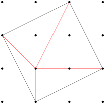
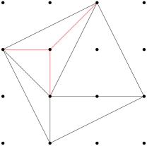
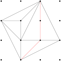
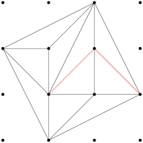
Figure 4: An illustration of the resolution of $\mathcal{C}_{5,2}$, following the process described in the proof of Theorem 4.3. In this case it consists of a sequence of four star subdivisions. Note that, once again, the coordinates used to make the graphics are different to those used in the text, in order to make the diagrams clearer.

To complete the proof that hyperconifold transitions occur between compact Calabi–Yau threefolds, we must argue that the local resolutions constructed above can always be glued into the compact geometries in an appropriate way (this is the step which can fail for small resolutions of a nodal threefold).

Theorem 4.5.

Let $X_{0}$ be a factorial Calabi–Yau threefold, smooth except for a singlehyperconifold singularity. Then $X_{0}$ admits a Calabi–Yau (i.e., projective and crepant)resolution.

Proof.

The singular point of $X_{0}$ has an analytic neighbourhood that is isomorphic to a neighbourhood of the singular point of $\mathcal{C}_{n,k}$. We can therefore analytically glue in the exceptional set of some projective resolution $\widehat{\mathcal{C}}_{n,k}$, and obtain a crepant analytic resolution $\pi:\widehat{X}\to X_{0}$. Being bimeromorphic to a variety, $\widehat{X}$ is an algebraic space.

Recall that a relative ample divisor for the resolution $\widehat{\mathcal{C}}_{n,k}\to\mathcal{C}_{n,k}$ can be constructed from components of the exceptional divisor $E$; let us choose such a divisor $D$, and abuse notation by also denoting by $D$ its image under the embedding $E\hookrightarrow\widehat{X}$. We now use the relative Nakai-Moishezon criterion for algebraic spaces [23, 24]: $D$ is $\pi$-ample if and only if $D^{\dim V}\cdot V>0$ for all irreducible closed subspaces $V$ for which $\pi(V)$ is a point. The only such $V$ are subspaces of the exceptional set $E$, and we know that $D$ is positive on these, since it is a relative ample divisor for $\widehat{\mathcal{C}}_{n,k}\to\mathcal{C}_{n,k}$. Therefore $D$ is also $\pi$-ample, so $\widehat{X}$ is projective. ∎

4.1.1 The local ample/Kähler cone

I will now introduce some terminology which is useful for discussing resolutions of isolated singularities, including hyperconifolds.

Definition.

Let $X_{0}$ be a variety, smooth except at one point, and let $\pi:\widehat{X}\to X_{0}$ be a (not necessarily algebraic) resolution map. Call the exceptional set $E$, and denote by $E_{1},\ldots,E_{N}$ its irreducible divisorial components. Then a local ample divisor for the resolution is a divisor $H_{L}=\sum_{i}t_{i}E_{i}$ such that for any subvariety $Y$ of $E$, $(H_{L})^{\dim Y}\cdot Y>0$. The local ample cone is the cone generated by numerical equivalence classes of local ample divisors; this may be empty.

A local ample divisor for a resolution $\pi$ is therefore simply a $\pi$-ample divisor that is supported only on the exceptional set; indeed, the definition comes from the relative Nakai-Moishezon criterion.

Remark.

In the case where $\widehat{X}$ is Calabi–Yau, ample ($\mathbb{R}$)-divisor classes are equivalent to Kähler classes, and we can equivalently talk about the local Kähler cone; this language is more natural for applications to string theory. The word ‘local’ has a double meaning: the local Kähler cone depends only on the fibre $E$ over the singular point of $X_{0}$, and it also describes the geometry of the Kähler cone in a neighbourhood of the face that corresponds to contracting $E$ to a point.

Lemma 4.6.

Let $X_{0}$ be a factorial projective variety with a unique singular point, and $\pi:\widehat{X}\to X_{0}$ an analytic resolution. Then $\widehat{X}$ is projective if and only if $\pi$ has a non-empty local ample cone.

Proof.

One direction is easy: we have already noted that if $H_{L}$ is a local ample divisor, it is a $\pi$-ample divisor. Then if we choose some ample divisor $H_{0}$ on $X_{0}$, $m\,\pi^{*}H_{0}+H_{L}$ will be ample on $\widehat{X}$ for all $m\gg 0$ [23].

Conversely, suppose $\widehat{X}$ admits an ample divisor $H$. Then we can write $H=\pi^{*}(H_{0})+H_{L}$, where $H_{0}$ is some class on $X_{0}$, and $H_{L}$ is supported only on the exceptional set. Since $X_{0}$ is factorial, $H_{0}$ has a representative not supported at the singular point (see Lemma 4.9); it follows that $\pi^{*}(H_{0})$ is zero on the exceptional set, and therefore, since $H$ is ample, $H_{L}$ must be a local ample divisor by the Nakai-Moishezon criterion. ∎

Remark.

When the singularity on $X_{0}$ is toric, and the resolution is also toric, there is a simpler condition for a local ample divisor: in this case, $H_{L}$ is a local ample divisor if and only if $H_{L}\cdot C>0$ for all toric curves $C$ in the exceptional set. This follows immediately from the relative ‘toric Kleiman condition’ [15].

Example 4.1 (Resolving $\mathcal{C}_{3,1}$).

There are two distinct crepant resolutions of $\mathcal{C}_{3,1}$, which is the unique $\mathbb{Z}_{3}$-hyperconifold; their toric diagrams are shown in Figure 5. We will see here that only the first has a non-empty local ample/Kähler cone, so any factorial projective variety containing this singularity admits exactly one crepant, projective resolution.

Figure 5: The two crepant resolutions of $\mathcal{C}_{3,1}$. The first has a non-empty local Kähler cone, while the second does not.

Case 1
Note that the first resolution corresponds to star subdivisions with respect to first one, then the other, of the interior points in the toric diagram for $\mathcal{C}_{3,1}$; we therefore expect a non-empty local ample cone. The exceptional set consists of two copies of the Hirzebruch surface $F_{1}$, glued along a common copy of $\mathbb{P}^{1}$ (this can be seen by utilising the ‘star construction’ of toric geometry [25]). Call the first surface $S_{1}$, and the second $S_{2}$, and define a putative local ample divisor $D_{L}=t_{1}S_{1}+t_{2}S_{2}$.

We can now evaluate the divisor $D_{L}$ against various curves in the resolution. To do so, note that by adjunction, and the fact that the ambient space $\widehat{\mathcal{C}}_{3,1}$ is Calabi–Yau, we have $K_{S_{i}}\sim S_{i}|_{S_{i}}$, so that if a curve $C$ is contained in $S_{i}$, we get $S_{i}\cdot C=K_{S_{i}}\cdot C=-2-C^{2}$, where the last equality follows from the fact that $S_{i}$ is a toric surface.

Each surface $S_{i}$ contains toric curves of self-intersection $0$, which intersect the other surface transversely at a single point. For such a curve $C_{1}\subset S_{1}$, we get $D_{L}\cdot C_{1}=-2t_{1}+t_{2}$, and similarly for $C_{2}\subset S_{2}$, we get $D_{L}\cdot C_{2}=t_{1}-2t_{2}$. Therefore $-2t_{1}+t_{2}>0$ and $t_{1}-2t_{2}>0$ are necessary conditions for a local ample divisor. The remaining toric curves only yield weaker inequalities, so the local ample/Kähler cone is given by

$$2t_{1}<t_{2}<\frac{1}{2}t_{1}~{}.$$

Note that this implies $t_{1}<0,t_{2}<0$.

Case 2
The second triangulation has an exceptional set consisting of two disjoint surfaces $S_{1},S_{2}$, each isomorphic to $\mathbb{P}^{2}$, and a rational curve $C$ which intersects each transversely at a single point. From considering the toric curves embedded in either $S_{1}$ or $S_{2}$, we get the conditions $t_{1}<0,t_{2}<0$. However, $D_{L}\cdot C=t_{1}+t_{2}$, so in this case the local ample/Kähler cone is empty.

4.2 Topological data

Given a hyperconifold transition $X\stackrel{{\scriptstyle\mathbb{Z}_{n}}}{{\rightsquigarrow}}\widehat{X}$, the results of this section will allow us to calculate the topological data of $\widehat{X}$ in terms of that of $X$.

4.2.1 Hodge numbers

Smooth Calabi–Yau threefolds have only two independent Hodge numbers undetermined by the Calabi–Yau conditions, which we can take to be $h^{1,1}$ and $h^{2,1}$. These quantities behave simply under hyperconifold transitions.

Theorem 4.7.

If $X\stackrel{{\scriptstyle\mathbb{Z}_{n}}}{{\rightsquigarrow}}\widehat{X}$ is a $\mathbb{Z}_{n}$-hyperconifold transition, then the Hodge numbers of $X$ and $\widehat{X}$ are related by

$$h^{1,1}(\widehat{X}) =h^{1,1}(X)+n-1~{},$$

$$h^{2,1}(\widehat{X}) =h^{2,1}(X)-1~{}.$$

Proof.

Due to the restricted Hodge diamond of a Calabi–Yau threefold, the topological Euler number is given simply by

$$\chi(X)=2\big{(}h^{1,1}(X)-h^{2,1}(X)\big{)}~{}.$$

The change in the Euler number is easy to calculate via the surgery picture of a transition. We delete a three-cycle homeomorphic to a lens space, which has $\chi=0$, and replace it with one of the toric spaces described in Section 4. The Euler number of a toric variety is equal to the number of top-dimensional cones in its fan; it follows that for any complete crepant resolution of a $\mathbb{Z}_{n}$-hyperconifold, the Euler number increases by $2n$. In terms of Hodge numbers,

$$\big{(}h^{1,1}(\widehat{X})-h^{1,1}(X)\big{)}-\big{(}h^{2,1}(\widehat{X})-h^{2,1}(X)\big{)}=n~{}.$$ (8)

Secondly, for a smooth Calabi–Yau threefold, the Hodge number $h^{1,1}$ is equal to the rank of the divisor class group, which allows us to calculate the first term. The intermediate singular variety $X_{0}$ is factorial by assumption, so its class group is isomorphic to that of $X$ (no new divisor classes are created on the singular variety). The resolution introduces an exceptional divisor with $n-1$ components, all linearly independent. Therefore

$$h^{1,1}(\widehat{X})-h^{1,1}(X)=n-1~{}.$$

Combining this with (8) gives the claimed relations. ∎

The decrease of $h^{2,1}$ by one can be understood as imposing one condition on the moduli of $X$ in order to form the hyperconifold singularity. We will see this very explicitly in Example 5.1.

4.2.2 The fundamental group

In the simplest case, a hyperconifold singularity develops when a generically-free group action develops at least one fixed point, so the corresponding singular variety will have a smaller fundamental group than the smooth members of the family. As we saw above, the resolution process involves gluing in a complete (reducible) toric surface, and these are simply-connected, so a hyperconifold transition will typically reduce the size of the fundamental group.

We will consider the situation where some general finite group $G$ acts freely on a Calabi–Yau threefold $\widetilde{X}$, which can be deformed until a cyclic subgroup develops a fixed point. Let $g\in G$ be a generator of this subgroup, and suppose $\tilde{x}\in\widetilde{X}$ is the fixed point. Then for any $h\in G$, we have $\big{(}hg^{k}h^{-1}\big{)}\big{(}h(\tilde{x})\big{)}=h(\tilde{x})$, so all elements conjugate to $g$, or any of its powers, also necessarily develop fixed points, which fill out the $G$-orbit of $\tilde{x}$. We might therefore expect the hyperconifold transition to ‘destroy’ the smallest normal subgroup containing $\langle g\rangle$—the normal closure $\langle g\rangle^{G}$. This can be made precise:

Theorem 4.8.

Let $t$ be a parameter, and $X_{t}=\widetilde{X}_{t}/G$ be a family of Calabi–Yau threefolds, smooth for $t\neq 0$, where each $\widetilde{X}_{t}$ is simply-connected. Suppose that $\widetilde{X}_{0}$ is smooth apart from a single $G$-orbit of nodes, and $X_{t}$ is smooth apart from a $\mathbb{Z}_{n}$-hyperconifold singularity, which is the image of the node(s) under the quotient map. If $\widehat{X}$ is a Calabi–Yau resolution of $X_{0}$, then $\pi_{1}(\widehat{X})\cong G/N$, where $N$ is the normal closure of the set of elements of $G$ which have fixed points on $\widetilde{X}_{0}$.

Proof.

Let $\tilde{x}\in\widetilde{X}_{0}$ be one of the nodes. Then $\widetilde{Y}=\widetilde{X}_{0}\setminus G\tilde{x}$ is smooth by assumption, and $G$ acts freely on it, yielding a smooth quotient space $Y=\widetilde{Y}/G$ with $\pi_{1}(Y)\cong G$. Note that, since all the nodes on $\widetilde{X}$ are identified by $G$, the space $Y$ is obtained from $X_{0}$ by removing the unique singular point.

Topologically, the resolution corresponds to gluing in a contractible neighbourhood $\Theta$ of the exceptional set, so that $\widehat{X}=Y\cup\Theta$. The result is a simple application of the Seifert-van Kampen theorem [26] to this decomposition, as I will now outline. Some neighbourhood of a $\mathbb{Z}_{n}$-hyperconifold singularity is homeomorphic to a cone over $S^{3}\times S^{2}/\mathbb{Z}_{n}$, which after deleting the tip is homotopy equivalent to $S^{3}\times S^{2}/\mathbb{Z}_{n}$; therefore $Y\cap\Theta\simeq S^{3}\times S^{2}/\mathbb{Z}_{n}$. Finally, note that $\Theta$ is at least homotopy-equivalent to a toric variety, corresponding to the resolutions constructed previously. Since the fans for these all contain at least one full-dimensional cone, they are all simply-connected [25]. So the data we have is

$$\hat{X}=Y\cup\Theta~{},~{}\pi_{1}(Y)\cong G~{},~{}\pi_{1}(\Theta)\cong\mathbf{1}~{},~{}\pi_{1}(Y\cap\Theta)\cong\mathbb{Z}_{n}~{}.$$

Since $Y$, $\Theta$ and $Y\cap\Theta$ are all path-connected, the result follows immediately from the Seifert-van Kampen theorem. ∎

There are examples of hyperconifold transitions which do not arise in exactly the way described in the Lemma. For instance, $X$ might already be simply-connected, yet undergo a hyperconifold transition to another simply-connected space; see [4] for some examples. The fundamental group can nevertheless always be computed using the simple technique of the proof above.

4.2.3 Intersection numbers

Finally, we can calculate the triple-intersection numbers of $\widehat{X}$ in terms of those of $X$. To do so, we will choose a basis consisting of divisors pulled back from $X_{0}$, and components of the exceptional divisor. The calculation of intersection numbers is made simple by the following lemma, which shows that we can choose a basis for the class group of $X_{0}$ which consists of divisors which do not intersect the singularity.

Lemma 4.9 (See, e.g., [27]).

Let $X_{0}$ be a factorial quasi-projective variety, and $\{x_{1},\ldots,x_{m}\}$ be some finite collection of points in $X_{0}$. Then, given any divisor $D$ on $X_{0}$, there exists a divisor $D^{\prime}\sim D$ which is not supported at any of the $x_{i}$.

We will now define a convenient basis of divisors in terms of which to compute the intersection numbers. Let $I,J,\ldots$ be indices running from $1$ to $h^{1,1}(\widehat{X})$, which we know from Section section 4.2.1 is equal to $h^{1,1}(X)+n-1$. We will split the basis into two parts; to this end, let the lower case latin indices $i,j,\ldots$ run from $1$ to $h^{1,1}(X)$, and greek indices $\alpha,\beta,\ldots$ run from $h^{1,1}(X)+1$ to $h^{1,1}(X)+n-1$.

Take a basis $\{D_{i}\}$ for the divisor class group of $X_{0}$, and let $\{\hat{D}_{i}\}$ be their pullbacks to $\widehat{X}$ under the resolution map. Then arbitrarily order the components of the exceptional divisor, and denote these by $\{\hat{D}_{\alpha}\}$. The total collection $\{\hat{D}_{I}\}$ defines a basis on $\widehat{X}$.

It is now straightforward to calculate all the intersection numbers of $\widehat{X}$:

Theorem 4.10.

Let $X\stackrel{{\scriptstyle\mathbb{Z}_{n}}}{{\rightsquigarrow}}\widehat{X}$ be a hyperconifold transition, with intermediate singular variety $X_{0}$. Then, in the basis for $H^{1,1}(X)$ defined above, the triple-intersection numbers $\hat{d}_{IJK}$ are

1. $\hat{d}_{ijk}=d_{ijk}$, where $d_{ijk}$ are the triple-intersection numbers on $X$ (and $X_{0}$).

2. $\hat{d}_{ij\alpha}=\hat{d}_{i\alpha\beta}=0$

3. $\hat{d}_{\alpha\beta\gamma}$ are the intersection numbers of the components of the exceptional divisor of $\widehat{\mathcal{C}}_{n,k}$, and can be calculated using standard toric techniques.

Proof.

By Lemma 4.9, the divisors $D_{i}$ can be chosen to miss the singularity of $X_{0}$. Since $\widehat{X}\cong X_{0}$ away from the exceptional divisor/singular point, the intersection numbers of the $\hat{D}_{i}$ are obviously the same as those of the $D_{i}$. To see that these are the same as the intersection numbers on $X$ (the smoothing of $X_{0}$), note that $X_{0}$ with the singularity deleted deforms to $X$ with a lens space deleted, and the divisors deform with the whole space. Intersection numbers are topological on smooth spaces, so $\hat{d}_{ijk}=d_{ijk}$.

If we choose the $D_{i}$ to miss the singularity as above, then it is clear that $\hat{D}_{i}\cap\hat{D}_{\alpha}=\mathrm{O}\raisebox{1.0pt}{/}\,~{}\forall~{}i,\alpha$, which immediately implies $\hat{d}_{ij\alpha}=\hat{d}_{i\alpha\beta}=0$.

The final statement is obvious, as intersection numbers are topological, and the resolved toric space $\widehat{\mathcal{C}}_{n,k}$ is homeomorphic to a neighbourhood of the exceptional divisor on $\widehat{X}$, of which the $\hat{D}_{\alpha}$ are components. ∎

5 Examples and applications

Hyperconifold transitions provide a method to construct new Calabi–Yau threefolds from existing ones. In fact, we already have one example for free: we saw in Section 1 that the $\mathbb{Z}_{5}$ quotient of the quintic can develop a $\mathbb{Z}_{5}$-hyperconifold singularity, and the results of Section 4 imply that this has a Calabi–Yau resolution $\widehat{X}$, and allow us to calculate its topological data. The $\mathbb{Z}_{5}$ quotient of the quintic has Hodge numbers $(h^{1,1},\,h^{2,1})=(1,21)$, and fundamental group $\mathbb{Z}_{5}$, which is destroyed by the transition. Therefore $(h^{1,1},\,h^{2,1})(\widehat{X})=(5,20)$ and $\pi_{1}(\widehat{X})\cong{\bf 1}$. This example was already given in [4], and is implicitly included in earlier work showing that geometric transitions connect all Calabi–Yau threefolds which are hypersurfaces in toric fourfolds [28].

In this section, I describe some examples of hyperconifold transitions, chosen tocomplement those previously given in [4]. In that paper, examples were given where the ambient space has multiple fixed points, allowing for ‘chains’ of hyperconifold transitions linking multiple manifolds, and a hyperconifold transition was also used to construct the first Calabi–Yau threefold with fundamental group $S_{3}$ (the permutation group on threeletters). I will also present two examples of hyperconifold singularities embedded in compact Calabi–Yau threefolds which are not factorial; in these cases, the singular varieties do not occur as the intermediate point of a hyperconifold transition, at least as defined in this paper.

Example 5.1 ($X^{1,3}\stackrel{{\scriptstyle\mathbb{Z}_{10}}}{{\rightsquigarrow}}X^{10,2}$).

Our first example will be very typical, and I will describe each step of the analysis in detail; this can then be used as a blueprint for any attempt to construct new Calabi–Yau manifolds via hyperconifold transitions.

We begin with a manifold $X$ with fundamental group $\mathbb{Z}_{10}\times\mathbb{Z}_{2}$, first constructed in [10]. The covering space, $\widetilde{X}$, is embeddable in a product of five copies of $\mathbb{P}^{1}$ as the complete intersection of two ‘quintilinear hypersurfaces’; its configuration matrix [7] is

$$\begin{matrix}\mathbb{P}^{1}\\ \mathbb{P}^{1}\\ \mathbb{P}^{1}\\ \mathbb{P}^{1}\\ \mathbb{P}^{1}\end{matrix}\!\left[\begin{matrix}1&1\\ 1&1\\ 1&1\\ 1&1\\ 1&1\end{matrix}\right]~{}.$$

Denote the two quintilinear polynomials by $p_{1},p_{2}$. If we take homogeneous coordinates $t_{i,a}$ on the ambient space, where $i\in\mathbb{Z}_{5}$ and $a\in\mathbb{Z}_{2}$, then we can define an action of the group $\mathbb{Z}_{10}\times\mathbb{Z}_{2}$ on the ambient space by allowing the generators of the two factor groups to act as

$$g_{10} :t_{i,a}\mapsto t_{i+1,a+1}~{};$$ (9)

$$g_{2} :t_{i,a}\mapsto(-1)^{a}t_{i,a}~{}.$$

If we demand that the polynomials transform equivariantly under this action, then the group will act on the corresponding manifolds $\widetilde{X}$; an appropriate choice of transformation rule is

$$g_{10} :p_{1}\mapsto p_{2}~{},~{}p_{2}\mapsto p_{1}~{};$$

$$g_{2} :p_{1}\mapsto p_{1}~{},~{}p_{2}\mapsto-p_{2}~{}.$$

To write down the most general polynomials satisfying these properties, it is convenient to first define the following quantities, which are invariant under the $\mathbb{Z}_{5}$ subgroup generated by $g_{10}^{2}$:

$$m_{abcde}:=\sum_{i}t_{i,a}t_{i+1,b}t_{i+2,c}t_{i+3,d}t_{i+4,e}~{}.$$

We now take the polynomials $p_{1},p_{2}$ to be

$$p_{1} =\frac{A_{0}}{5}m_{00000}+A_{1}m_{00011}+A_{2}m_{00101}+A_{3}m_{01111}~{},$$

$$p_{2} =\frac{A_{0}}{5}m_{11111}+A_{1}m_{11100}+A_{2}m_{11010}+A_{3}m_{10000}~{},$$

where the coefficients are arbitrary complex numbers. It can be checked that even these very restricted polynomials cut out a smooth manifold for generic choices of the coefficients; I will defer to [10] for the details of this step.

To establish the existence of a smooth quotient, we must also check that the group action on $\widetilde{X}$ is fixed-point-free. To do so, it is not necessary to check separately that every group element acts freely, because if $g\in G$ has a fixed point, then so do all its powers. A general element of $\mathbb{Z}_{10}\times\mathbb{Z}_{2}$ can be written as $g_{10}^{k}g_{2}^{a}$, with $0\leq k\leq 9$ and $0\leq a\leq 1$. Depending on the values of $k$ and $a$, some power of this will be $g_{10}^{2},g_{10}^{5},g_{10}^{5}g_{2}$, or $g_{2}$, so we need only check that these elements act freely. The fixed points of these elements are listed in the following table:

Element	Fixed points
$g_{10}^{2}$	$[t_{i,0}:t_{i,1}]=[t_{0,0}:t_{0,1}]~{}\forall~{}i$
$g_{10}^{5}$	$t_{i,a}=\pm t_{i,a+1}$ (sign can depend arbitrarily on $i$)
$g_{10}^{5}g_{2}$	$t_{i,a}=\pm\text{i}t_{i,a+1}$ (sign can depend arbitrarily on $i$)
$g_{2}$	For each $i$, either $t_{i,0}=0$ or $t_{i,1}=0$

In the case of $g_{10}^{2}$, the fixed points form an embedded copy of $\mathbb{P}^{1}$, and the two polynomials become quintics in this $\mathbb{P}^{1}$, which do not have simultaneous solutions for arbitrary coefficients. The fixed points of the other elements are all isolated, and at each one, the polynomials $p_{1},p_{2}$ evaluate to non-trivial linear combinations of the coefficients. We conclude that for generic choices of the coefficients, the group action is free. We therefore obtain a smooth Calabi–Yau quotient, $X^{1,3}$, with fundamental group $\mathbb{Z}_{10}\times\mathbb{Z}_{2}$. The three complex structure moduli correspond to the three degrees of freedom in the coefficients of $p_{1},p_{2}$, up to scale.

We seek a $\mathbb{Z}_{10}$-hyperconifold transition, so wish to specialise the choice of polynomials so that $\widetilde{X}$ contains a fixed point of the $\mathbb{Z}_{10}$ subgroup. Referring to the table above, and noting that some point $\tilde{x}\in\widetilde{X}$ is fixed by $g_{10}$ if and only if it is fixed by $g_{10}^{2}$ and $g_{10}^{5}$, we see that there are exactly two such points, given by $[t_{i,0}:t_{i,1}]=[1:\pm 1]$ for all $i$ (with the same sign chosen for each value of $i$). These are exchanged by $g_{2}$, so the symmetric $\widetilde{X}$ will contain one if and only if it contains the other. At these points, we have $p_{1}=\pm p_{2}=A_{0}+5A_{1}+5A_{2}+5A_{3}$. To be concrete, let us choose the following values of the coefficients, which ensure that this quantity vanishes (and also that the polynomials do not vanish at the other fixed points in the ambient space): $(A_{0},A_{1},A_{2},A_{3})=(-30,1,2,3)$.

With the aid of a computer algebra package, it can be checked that for the above choice of coefficients, $\widetilde{X}$ is singular at precisely the two fixed points of $g_{10}$. Our next task is to investigate the nature of these singularities. To this end, we choose local coordinates centred on one of the fixed points (the other is identical, thanks to the $g_{2}$ symmetry exchanging them): set $t_{i,0}=1$ for all $i$, and $t_{i,1}=1+\epsilon_{i}$. We then expand the polynomials $p_{1},p_{2}$ to quadratic order in $\vec{\epsilon}$:

$$p_{1}= 18\epsilon_{0}+18\epsilon_{1}+18\epsilon_{2}+18\epsilon_{3}+18\epsilon_{4}+10\epsilon_{0}\epsilon_{1}+11\epsilon_{0}\epsilon_{2}$$

$$+11\epsilon_{0}\epsilon_{3}+10\epsilon_{0}\epsilon_{4}+10\epsilon_{1}\epsilon_{2}+11\epsilon_{1}\epsilon_{3}+11\epsilon_{1}\epsilon_{4}+10\epsilon_{2}\epsilon_{3}+11\epsilon_{2}\epsilon_{4}+10\epsilon_{3}\epsilon_{4}+\mathcal{O}(\epsilon^{3})$$

$$p_{2}= -18\epsilon_{0}-18\epsilon_{1}-18\epsilon_{2}-18\epsilon_{3}-18\epsilon_{4}-26\epsilon_{0}\epsilon_{1}-25\epsilon_{0}\epsilon_{2}$$

$$-25\epsilon_{0}\epsilon_{3}-26\epsilon_{0}\epsilon_{4}-26\epsilon_{1}\epsilon_{2}-25\epsilon_{1}\epsilon_{3}-25\epsilon_{1}\epsilon_{4}-26\epsilon_{2}\epsilon_{3}-25\epsilon_{2}\epsilon_{4}-26\epsilon_{3}\epsilon_{4}+\mathcal{O}(\epsilon^{3})$$

Note that $p_{1}+p_{2}$ has no linear term, and is invariant under the action of $g_{10}$. To proceed, we can solve (say) $p_{2}=0$ for $\epsilon_{0}$ as a power series in the other variables, and substitute this into $p_{1}+p_{2}$ up to order $\epsilon^{2}$. I will spare the reader the ugly details, but one can check that the resulting leading-order terms constitute a non-degenerate quadratic form, invariant under the $g_{10}$ action. So our singularity is analytically isomorphic to the conifold, and the quotient space has a $\mathbb{Z}_{10}$-hyperconifold singularity.

To determine the $\mathbb{Z}_{10}$ action on the singularity, we linearise the action on the local coordinates. In terms of the $\epsilon_{i}$, (9) becomes

$$g_{10}=[1:1+\epsilon_{i}]\mapsto[1+\epsilon_{i+1}:1]\sim\left[1:\frac{1}{1+\epsilon_{i+1}}\right]=[1:1-\epsilon_{i+1}+\mathcal{O}(\epsilon^{2})]~{}.$$

In other words $\epsilon_{i}\mapsto-\epsilon_{i+1}$ for $i=1,2,3$. For $i=4$, we have $\epsilon_{4}\mapsto-\epsilon_{0}$, but $\epsilon_{0}$ is not amongst our local coordinates; we have solved $p_{2}=0$ to obtain $\epsilon_{0}=-\epsilon_{1}-\epsilon_{2}-\epsilon_{3}-\epsilon_{4}+\mathcal{O}(\epsilon^{2})$, so the $g_{10}$ action effects $\epsilon_{4}\mapsto\epsilon_{1}+\epsilon_{2}+\epsilon_{3}+\epsilon_{4}$. The linearised action of $g_{10}$ is therefore given by the matrix

$$\left(\begin{array}[]{rrrr}0&-1&0&0\\ 0&0&-1&0\\ 0&0&0&-1\\ 1&1&1&1\end{array}\right)~{}.$$

The eigenvalues of this matrix are $\zeta,\zeta^{3},\zeta^{7},\zeta^{9}$, where $\zeta=e^{2\pi\text{i}/10}$, so the singularity on the quotient space is described by the hyperconifold $\mathcal{C}_{10,3}$.

We conclude that, over the locus $A_{0}+5A_{1}+5A_{2}+5A_{3}=0$, the space $X^{1,3}$ develops a hyperconifold singularity, modelled on $\mathcal{C}_{10,3}$. By 4.2, it is factorial, and by 4.5 we can therefore obtain a new Calabi–Yau manifold by deleting the singular point, and gluing in any geometry described by a star subdivision of the fan for $\mathcal{C}_{10,3}$. One such subdivision is shown in Figure 6.

We began with a manifold which has fundamental group $\mathbb{Z}_{10}\times\mathbb{Z}_{2}$ and Hodge numbers $(h^{1,1},\,h^{2,1})=(1,3)$, and constructed a $\mathbb{Z}_{10}$-hyperconifold transition by allowing the $\mathbb{Z}_{10}$ factor to develop a fixed point on the covering space. According to the formulae of Theorem 4.7 and Theorem 4.8, the new manifold has Hodge numbers $(h^{1,1},\,h^{2,1})=(10,2)$, and fundamental group $\mathbb{Z}_{2}$.

Figure 6: One projective crepant resolution of $\mathcal{C}_{10,3}$, given by a sequence of star subdivisions. A different example, in which the first subdivision is with respect to the central lattice point, is given in [4].

Example 5.2 (A non-normal subgroup).

In [8], Braun found families of smooth Calabi–Yau threefolds on which the non-Abelian group $\mathrm{Dic}_{3}\cong\mathbb{Z}_{3}\rtimes\mathbb{Z}_{4}$ acts freely. There is only one non-trivial semi-direct product of this form; the group presentation is

$$\mathrm{Dic}_{3}\cong\langle g_{3},g_{4}~{}|~{}g_{3}^{3}=g_{4}^{4}=e~{},~{}g_{4}^{-1}g_{3}g_{4}=g_{3}^{2}\rangle,$$

where $e$ is the identity. It is easy to see that the $\mathbb{Z}_{2}$ subgroup generated by $g_{4}^{2}$ is normal, and that $\mathrm{Dic}_{3}/\mathbb{Z}_{2}\cong S_{3}$. This fact was used in [14] to construct, via a $\mathbb{Z}_{2}$-hyperconifold transition, the first known Calabi–Yau threefold with fundamental group $S_{3}$.

We can instead construct a $\mathbb{Z}_{4}$-hyperconifold transition from the space $X^{1,4}=\widetilde{X}^{8,44}/\mathrm{Dic}_{3}$ [30]. This can indeed be done; the details can be checked following the same procedure as in the last example, and we obtain a new smooth Calabi–Yau $X^{4,3}$. Because the subgroup $\mathbb{Z}_{4}$ is not normal, we must compute its normal closure in order to find the fundamental group of $X^{4,3}$.

Note that $g_{3}g_{4}g_{3}^{-1}=g_{4}g_{3}$, and between them, $g_{4}$ and $g_{4}g_{3}$ generated all of $\mathrm{Dic}_{3}$. Therefore $\mathbb{Z}_{4}^{\mathrm{Dic}_{3}}=\mathrm{Dic}_{3}$; Theorem 4.8 then implies that $\pi_{1}(X^{4,3})$ is trivial.

Example 5.3 (‘Swiss-cheese’ manifolds from hyperconifold transitions).

A popular idea in string theory model building is the ‘LARGE volume scenario’ in Type IIB [31, 32, 33]. This requires a three-dimensional Calabi–Yau manifold admitting a particular limit in Kähler moduli space. It must be possible to take the overall volume of the manifold to infinity while certain prime divisors remain of finite size. Such spaces have been dubbed ‘Swiss-cheese manifolds’.

Hyperconifold transitions provide an easy and systematic way to construct such Swiss-cheese manifolds, which complements the use of the several known ad-hoc examples, and the computationally-intensive search technique outline in [34].

Example 5.4 (A non-factorial hyperconifold with a Calabi–Yau resolution).

In [35], atechnique was introduced for finding embeddings of certain toric singularities into compactCalabi–Yau manifolds. Briefly, let $Y$ be an affine toric Calabi–Yau. To embed $Y$ in acompact Calabi–Yau, the authors of [35] seek a compact toric Fano fourfold whichcontains an affine patch $Y\times\mathbb{C}^{*}$, such that a generic anti-canonical hypersurface intersects it in $Y\times\{\text{pt}\}$.

Using the technique described above, the $\mathbb{Z}_{3}$-hyperconifold $\mathcal{C}_{3,1}$ was embedded in a compact Calabi–Yau threefold. The ambient toric space is described by the face fan of the four-dimensional polytope with the following vertices:

$$\begin{array}[]{rrrrrrr}v_{1}&v_{2}&v_{3}&v_{4}&v_{5}&v_{6}&v_{7}\\ 0&0&0&1&0&-1&0\\ 0&0&\phantom{-}1&\phantom{-}1&-1&0&\phantom{-}2\\ -1&0&1&2&2&2&2\\ 0&-1&1&3&3&3&3\end{array}$$

It is clear that the last four vertices lie on the same two-dimensional face, and thecorresponding affine patch is precisely $\mathcal{C}_{3,1}\times\mathbb{C}^{*}$ (to see this, it helps to sketch thepositions of the vertices in the plane). It follows that the divisors which correspond to these vertices are non-Cartier. Indeed, they are simply $D_{i}\times\mathbb{C}^{*}$, where the $D_{i}$ are the four toric (non-Cartier) divisors on $\mathcal{C}_{3,1}$, and therefore also restrict to non-Cartier divisors on the Calabi–Yau hypersurface, demonstrating that it is not factorial.

A smooth Calabi–Yau resolution is also constructed, and the corresponding localresolution of $\mathcal{C}_{3,1}$ is the ‘wrong’ one as discussed in Example 4.1. There is no contradiction,because the singular variety is not factorial. Presumably there is no smoothing of the singular variety, so that this example does not correspond to a transition.

Example 5.5 (A smoothable non-factorial hyperconifold).

In [38], Calabi–Yau manifolds with Hodge numbers $(h^{1,1},\,h^{2,1})=(1,1)$ were constructed via free actions of groups of order twenty-four on a simply-connected manifold with $(h^{1,1},\,h^{2,1})=(20,20)$. The three different groups have a common $\mathbb{Z}_{3}$ subgroup (this is not maximal; the intersection of the three groups is $\mathbb{Z}_{6}$), and all act freely on the same one-parameter family.

One might be interested in finding $\mathbb{Z}_{3}$-hyperconifold transitions from these spaces, toconstruct new (rigid) Calabi–Yau manifolds with Hodge numbers $(h^{1,1},\,h^{2,1})=(3,0)$.However, if we arrange for $X^{1,1}$ to develop a $\mathbb{Z}_{3}$-hyperconifold, it in fact develops four such singularities. The reason for this is the extra symmetry; the one-parameter family has a larger symmetry group than just the order-24 quotient group, and nodes must fall into orbits under the larger symmetry group.

If we specialise the hypersurface to intersect the $\mathbb{Z}_{3}$-fixed points, then its equationsimplifies as follows. Take toric coordinates $t_{1},t_{2},t_{3},t_{4}$ on the four-torus, and definecoordinates centred on one $\mathbb{Z}_{3}$-fixed point by letting $t_{i}=e^{2\pi\text{i}/3}+x_{i}$. Then the hypersurface equation becomes

$$x_{1}x_{4}f_{1}(\vec{x})+x_{2}x_{3}f_{2}(\vec{x})=0~{},$$

for certain polynomials $f_{1},f_{2}$. Clearly, the hypersurface is not factorial in this case; one example of a non-Cartier divisor is $x_{1}=x_{2}=0$.

Our previous arguments for a Calabi–Yau resolution therefore fail. However, we can certainly obtain resolutions which are complex manifolds with $c_{1}=0$, by removing the four $\mathbb{Z}_{3}$-hyperconifolds and gluing in crepant resolutions of $\mathcal{C}_{3,1}$. The resulting spaces have Euler number $0+4\times 6=24$. I have been unable to establish whether there is a projective resolution among these; if so, it would correspond to a rigid Calabi–Yau manifold with Hodge numbers $(h^{1,1},\,h^{2,1})=(12,0)$. The number $h^{1,1}=12$ must arise from the one Cartier divisor class on $X^{1,1}$, the eight ‘local’ divisors which project to the singular points (two to each), and the classes of the proper transforms of three independent non-Cartier divisors on the singular space.

So this is a more complicated transition than simply a $\mathbb{Z}_{3}$-hyperconifold transition (or even three such transitions ‘performed simultaneously’).

Appendix A The exceptional hyperconifold

In Section 3, we ignored the possibility that the generator of a hyperconifold quotient group might have a non-trivial projection onto the $\mathbb{Z}_{2}$ factor of the symmetry group. In this appendix we will show that there is only one such case—another $\mathbb{Z}_{4}$-hyperconifold, distinct from $\mathcal{C}_{4,1}$.

Lemma A.1.

Up to isomorphism, the only hyperconifold singularity for which the quotient group has a non-trivial projection to the $\mathbb{Z}_{2}$ factor in (7) is given by the following $\mathbb{Z}_{4}$ action:

$$(y_{1},y_{2},y_{3}y_{4})\mapsto(\text{i}y_{1},y_{3},-y_{2},\text{i}y_{4})~{}.$$

Proof.

The generator of the $\mathbb{Z}_{2}$ factor in the symmetry group of the conifold acts on the homogeneous coordinates as $z_{1}\leftrightarrow z_{3},z_{2}\leftrightarrow z_{4}$, and therefore on the hypersurface coordinates simply as $y_{2}\leftrightarrow y_{3}$. Inspecting the expression (3) for the holomorphic $(3,0)$-form, we see that it is odd under this transformation: $\Omega\mapsto-\Omega$. Therefore, to obtain a hyperconifold singularity, we must compose it with some torus transformation under which $\Omega$ is also odd.

We have already seen that $\Omega$ transforms the same way as the polynomial $p=y_{1}y_{4}-y_{2}y_{3}$ under the torus action, so we seek finite-order torus elements under which the monomials $y_{1}y_{4}$ and $y_{2}y_{3}$ are each odd. When combined with the order-two transformation above, this leads us to a subgroup generated by an element of the form

$$g:(y_{1},y_{2},y_{3},y_{4})\mapsto(\eta y_{1},\eta^{k}y_{3},\eta^{n-k}y_{2},\eta^{n-1}y_{4})~{},$$ (10)

where $\eta=e^{\pi\text{i}/n}$ for some $n$, and $0<k<n$.

Now we must impose that the origin is the only fixed point of any of the group elements. First, consider the group action on the linear subspace parametrised by $(y_{2},y_{3})$; this is given by the matrix

$$\left(\begin{array}[]{ll}0&\eta^{k}\\ \eta^{n-k}&0\end{array}\right)~{}.$$

We can see immediately that the fourth power of this matrix is the identity, and therefore that $g^{4}$ fixes, for example, the whole line $\{(0,y_{2},0,0\}\subset\mathcal{C}$, irrespective of our choice of $n,k$. Since we require that any non-trivial group element fixes only the origin, we conclude that $g$ must have order four. Therefore $\eta=\text{i}$, and $k=0$ or $k=2$. The coordinate redefinition $y_{2}\leftrightarrow y_{3}$ exchanges these two possibilities while leaving the polynomial $p$ invariant, so without loss of generality, we may assume that $k=0$. ∎

Remark.

The polynomial $p$ is odd under the generator of the action described above. This singularity therefore does not arise from the limit of a free group action on the deformed conifold given by $p+t=0$, $t\neq 0$.

References

- [1] C. H. Clemens, “Double solids,” Advances in mathematics 47 no. 2, (1983) 107–230.
- [2] F. Hirzebruch, “Some examples of threefolds with trivial canonical bundle. Notes by J. Werner,” F. Hirzebruch, Collected Papers II (1985) 757–770.
- [3] R. Davies, “Quotients of the conifold in compact Calabi-Yau threefolds, and new topological transitions,” Adv.Theor.Math.Phys. 14 (2010) 965–990, arXiv:0911.0708 [hep-th].
- [4] R. Davies, “Hyperconifold Transitions, Mirror Symmetry, and String Theory,” Nucl.Phys. B850 (2011) 214–231, arXiv:1102.1428 [hep-th].
- [5] P. Candelas, G. T. Horowitz, A. Strominger, and E. Witten, “Vacuum Configurations for Superstrings,” Nucl.Phys. B258 (1985) 46–74.
- [6] E. Witten, “New Issues in Manifolds of SU(3) Holonomy,” Nucl. Phys. B268 (1986) 79.
- [7] P. Candelas, A. M. Dale, C. A. Lutken, and R. Schimmrigk, “Complete Intersection Calabi-Yau Manifolds,” Nucl. Phys. B298 (1988) 493.
- [8] V. Braun, “On Free Quotients of Complete Intersection Calabi-Yau Manifolds,” JHEP 1104 (2011) 005, arXiv:1003.3235 [hep-th].
- [9] M. Schlessinger, “Rigidity of quotient singularities,” Inventiones mathematicae 14 no. 1, (1971) 17–26.
- [10] P. Candelas and R. Davies, “New Calabi-Yau Manifolds with Small Hodge Numbers,” Fortsch. Phys. 58 (2010) 383–466, arXiv:0809.4681 [hep-th].
- [11] M. F. Atiyah and R. Bott, “A Lefschetz fixed point formula for elliptic differential operators,” Bull. Amer. Math. Soc. 72 (1966) 245–250.
- [12] M. F. Atiyah and R. Bott, “A Lefschetz fixed point formula for elliptic complexes: II. Applications,” Ann. of Math. 88 (1968) 451–491.
- [13] P. Candelas, P. S. Green, and T. Hubsch, “Rolling Among Calabi-Yau Vacua,” Nucl. Phys. B330 (1990) 49.
- [14] R. Davies, “The Expanding Zoo of Calabi-Yau Threefolds,” Adv.High Energy Phys. 2011 (2011) 901898, arXiv:1103.3156 [hep-th].
- [15] D. A. Cox, J. B. Little, and H. K. Schenck, Toric Varieties, vol. 124 of Graduate Studies in Mathematics. American Mathematical Society, 2011.
- [16] P. Candelas and X. C. de la Ossa, “Comments on Conifolds,” Nucl. Phys. B342 (1990) 246–268.
- [17] J. Evslin and S. Kuperstein, “Trivializing and Orbifolding the Conifold’s Base,” JHEP 04 (2007) 001, hep-th/0702041.
- [18] D. R. Morrison, “Through the looking glass,” in *Montreal 1995, Mirror symmetry 3* (1995) 263–277, alg-geom/9705028v2.
- [19] M. Gross, “Examples of Special Lagrangian Fibrations,” in *Symplectic Geometry and Mirror Symmetry: Proceedings of the 4th KIAS Annual International Conference* (2001) 81–110, math/0012002.
- [20] V. V. Batyrev, “Dual polyhedra and mirror symmetry for Calabi-Yau hypersurfaces in toric varieties,” J.Alg.Geom. 3 (1994) 493–545, alg-geom/9310003.
- [21] R. Friedman, “Simultaneous Resolution of Threefold Double Points,” Math. Ann. 274 (1986) 671–689.
- [22] R. Friedman, “On threefolds with trivial canonical bundle,” Proc. Symposia Pure Math 53 (1991) 103–134.
- [23] R. Lazarsfeld, Positivity in Algebraic Geometry I: Classical Setting: Line Bundles and Linear Series. Ergebnisse der Mathematik und ihrer Grenzgebiete. 3. Folge A Series of Modern Surveys in Mathematics. Springer, 2004.
- [24] J. Kollár, “Projectivity of complete moduli,” Journal of Differential Geometry 32 no. 1, (1990) 235–268.
- [25] W. Fulton, Introduction to Toric Varieties. Princeton University Press, 1993.
- [26] A. Hatcher, Algebraic Topology. Cambridge University Press, 2002.
- [27] I. R. Shafarevich, Basic Algebraic Geometry, vol. 1. Springer-Verlag, second ed., 1994.
- [28] M. Kreuzer and H. Skarke, “Complete classification of reflexive polyhedra in four-dimensions,” Adv.Theor.Math.Phys. 4 (2002) 1209–1230, hep-th/0002240.
- [29] Wolfram Research, Inc., Mathematica, version 8.0. Wolfram Research, Inc., 2010.
- [30] V. Braun, P. Candelas, and R. Davies, “A Three-Generation Calabi-Yau Manifold with Small Hodge Numbers,” Fortsch. Phys. 58 (2010) 467–502, arXiv:0910.5464 [hep-th].
- [31] V. Balasubramanian, P. Berglund, J. P. Conlon, and F. Quevedo, “Systematics of moduli stabilisation in Calabi-Yau flux compactifications,” JHEP 0503 (2005) 007, arXiv:hep-th/0502058 [hep-th].
- [32] J. P. Conlon, F. Quevedo, and K. Suruliz, “Large-volume flux compactifications: Moduli spectrum and D3/D7 soft supersymmetry breaking,” JHEP 0508 (2005) 007, arXiv:hep-th/0505076 [hep-th].
- [33] M. Cicoli, J. P. Conlon, and F. Quevedo, “General Analysis of LARGE Volume Scenarios with String Loop Moduli Stabilisation,” JHEP 0810 (2008) 105, arXiv:0805.1029 [hep-th].
- [34] J. Gray, Y.-H. He, V. Jejjala, B. Jurke, B. D. Nelson, and J. Simón, “Calabi-Yau Manifolds with Large Volume Vacua,” Phys.Rev. D86 (2012) 101901, arXiv:1207.5801 [hep-th].
- [35] V. Balasubramanian, P. Berglund, V. Braun, and I. Garcia-Etxebarria, “Global embeddings for branes at toric singularities,” JHEP 1210 (2012) 132, arXiv:1201.5379 [hep-th].
- [36] J. P. Gauntlett, D. Martelli, J. Sparks, and D. Waldram, “Sasaki-Einstein metrics on S**2 x S**3,” Adv.Theor.Math.Phys. 8 (2004) 711–734, hep-th/0403002.
- [37] D. Martelli and J. Sparks, “Toric geometry, Sasaki-Einstein manifolds and a new infinite class of AdS/CFT duals,” Commun.Math.Phys. 262 (2006) 51–89, hep-th/0411238.
- [38] V. Braun, “The 24-Cell and Calabi-Yau Threefolds with Hodge Numbers (1,1),” JHEP 1205 (2012) 101, arXiv:1102.4880 [hep-th].