Enhancing entanglement trapping by weak measurement and quantum measurement reversal

Abstract

In this paper, we propose a scheme to enhance trapping of entanglement of two qubits in the environment of a photonic band gap material. Our entanglement trapping promotion scheme makes use of combined weak measurements and quantum measurement reversals. The optimal promotion of entanglement trapping can be acquired with a reasonable finite success probability by adjusting measurement strengths.

I Introduction

Entanglement is a vital resource for quantum information processing such as quantum computation, quantum metrology and quantum communication Nielsen-Chuang . However, realistic quantum systems are never completely isolated from the environment. The inevitable interaction between a system and its environment leads to quantum decoherence Zurek . For an open multipartite quantum system, decoherence leads to degradation of entanglement and, for some cases, entanglement sudden death (ESD) Yu ; Almeida ; Laurat ; Xu ; Zhang ; ParaoanuGS . Thus, tackling decoherence for entanglement protection is a critical issue for quantum information processing. It is therefore of interest to examine the possible schemes that can lead to promotion or preservation of entanglement.

At present, many methods have been proposed to protect entanglement from decoherence and to increase the entanglement such as by entanglement distillation Bennett ; Pan ; Dong . Quantum Zeno effect Facchi can also be used to manipulated the decoherence process, but in this method some special measurements should be performed very frequently to freeze the quantum state in order to prevent the degradation of entanglement. We can also deal with decoherence by introducing the decoherence-free subspace Lidar ; Kwiat . However, the decoherence-free subspace requires the interaction Hamiltonian to have an appropriate symmetry, which might not always be present. In most cases, the energy dissipation of individual subsystems of a composite system is responsible for the entanglement degradation. Hence, methods that can prevent the decay of the excited-state population would be applicable. One way widely applied is to place the qubits in a structured environment, say, microcavity Osnaghi ; Hagley or in the photonic band gap of photonic crystals Konopka ; Zhangxia ; LoFrancoB . In particular, in the photonic band gaps so as to inhibit spontaneous emission, a trapping state is formed and permanent entanglement is observed. This phenomenon, known as ”entanglement trapping” LoFranco ; Lazarou ; Bellomo , can lead to effective long-time entanglement protection.

Recently, it is shown that weak measurement and quantum measurement reversal can effectively suppress amplitude-damping decoherence for a single qubit Korotkov ; Paraoanu ; Lee . For the case of two qubits, remarkably, the weak measurement and quantum measurement reversal can increase the entanglement, and even can avoid entanglement sudden death Kimys , see also ManXiaAn . For weak measurements Korotkov1 , the outcome cannot determine the state of the measured system precisely and therefore does not totally collapse the state of the system. The correspondingly partial information is drawn from the measurement yielding a nonunitary, nonprojective transformation of the quantum state. Measurement reversal Katz1 ; Korotkov2 is a probabilistic reversal of a partial quantum measurement, and only certain outcomes of the measurement keep the full information of the initial state and are possible to reverse. The probability of success decreases with increasing strength of measurement, so that the reversible measurement has zero probability for a traditional projective measurement. Probabilistic reversal with a weak measurement has already been demonstrated on a superconducting phase qubit Katz1 , as well as on a photonic qubit KimYH .

Then, it will be interesting to know whether the method of weak measurement and quantum measurement reversal can be applied to enhance the entanglement trapping in a common photonic band gap. In this article, we show that this method indeed works for this system, and in particular, the entanglement can be trapped in a higher level. The success of this scheme is based on the fact that weak measurement can be reversed and thus the amplitude-damping, the main decoherence in photonic band gap, can be suppressed. We remark that this scheme does not need frequent measurements compared with quantum Zeno effect in suppressing decoherence.

This paper is organized as follows. In Sec. II, we describe the model of two qubits interacting with environment of a photonic band gap. We adopt the pseudomode approach to derive their evolution process. In Sec. III, we propose the scheme to enhance the entanglement trapping by using weak measurement and quantum measurement reversal. Finally, in Sec. IV, we present the feasibility of the experimental implementation of this scheme, and provide a brief conclusion.

II Physical model and dynamics process

We consider a two-qubit system interacting with a common zero-temperature bosonic reservoir. Our chosen specific system consists of two identical two-level atoms ($A$ and $B$) interacting with a common photonic band gap. The dynamics of two qubits coupled to the reservoir modes can be describe by the Hamiltonian

$$H=\omega_{0}\sigma^{A}_{+}\sigma^{A}_{-}+\omega_{0}\sigma^{B}_{+}\sigma^{B}_{-}+\sum_{k}\omega_{k}a^{{\dagger}}_{k}a_{k}+[(\sigma^{A}_{+}+\sigma^{B}_{+})\sum_{k}g_{k}a_{k}+h.c.],$$ (1)

where $a^{{\dagger}}_{k}$, $a_{k}$ are the creation and annihilation operators of quanta of the reservoir, $\sigma^{j}_{+}=|e_{j}{\rangle}{\langle}g_{j}|$, $\sigma^{j}_{-}=|g_{j}{\rangle}{\langle}e_{j}|$ and $\omega_{0}$ are the inversion operators and transition frequency of the $j$-th qubit (j=$A$, $B$); $\omega_{k}$ and $g_{k}$ are the frequency of the mode $k$ of the reservoir and its coupling strength with two qubits.

In order to find the dynamics of two qubits, we solve the master equation by using the pseudomode approach Garraway ; Garraway1 ; Garraway2 . This exact master equation describes the coherent interaction between the qubits and the pseudomodes in presence of decay of the pseudomodes due to the interaction with a Markovian reservoir. The number of the pseudomodes relies on the shape of the reservoir spectral distribution. We focus on an idealized model Garraway of a photonic band gap (or photon density of states gap) in which both Lorentzians are centered at the same frequency, and one of them is given a negative weighting, so that $D(\omega)=\frac{W_{1}\Gamma_{1}}{(\omega-\omega_{c})^{2}+(\Gamma_{1}/2)^{2}}-\frac{W_{2}\Gamma_{2}}{(\omega-\omega_{c})^{2}+(\Gamma_{2}/2)^{2}}$, where the weights of the two Lorentzians are such that $W_{1}-W_{2}=1$. The effect of the Lorentzian with negative weight is to introduced a dip into the density of states function $D(\omega)$ where the coupling of the qubit will be inhibited. $\omega_{c}$ is the center of the spectrum, and $\Gamma_{1}$, $\Gamma_{2}$ are the full widths at half maximum of two Lorentzians, respectively. There are two poles in $D$ which are located at $\omega_{c}-i\Gamma_{1}/2$ and $\omega_{c}-i\Gamma_{2}/2$, and there is a change in sign of the residues of $D$ between these poles. So the photonic band gap exists two pseudomodes $a_{1}$ and $a_{2}$ decaying with decay rates $\Gamma^{\prime}_{1}=W_{1}\Gamma_{2}-W_{2}\Gamma_{1}$ and $\Gamma^{\prime}_{2}=W_{1}\Gamma_{1}-W_{2}\Gamma_{2}$ respectively. Two qubits do not couple to the first pseudomode $a_{1}$ at all, they only interacts with the second pseudomode $a_{2}$ (the strength of the coupling $\Omega$) which is coupled to the first one (the strength of the coupling $V=\sqrt{W_{1}W_{2}}(\Gamma_{1}-\Gamma_{2})/2$), and both pseudomodes are leaking into independent Markovian environments. The exact pseudomode master equation associated with the band-gap model is given by

$$\frac{d\rho}{dt}= - i[H_{eff},\rho]-\frac{\Gamma^{\prime}_{1}}{2}(a^{{\dagger}}_{1}a_{1}\rho-2a_{1}{\rho}a^{{\dagger}}_{1}+{\rho}a^{{\dagger}}_{1}a_{1})-\frac{\Gamma^{\prime}_{2}}{2}(a^{{\dagger}}_{2}a_{2}\rho-2a_{2}{\rho}a^{{\dagger}}_{2}+{\rho}a^{{\dagger}}_{2}a_{2}),$$ (2)

here, the effective Hamiltonian of the total system in the pseudomode theory can be expressed

$$H_{eff} = \omega_{0}\sigma^{A}_{+}\sigma^{A}_{-}+\omega_{0}\sigma^{B}_{+}\sigma^{B}_{-}+\omega_{c}a^{{\dagger}}_{1}a_{1}+\omega_{c}a^{{\dagger}}_{2}a_{2}+\Omega[a_{2}(\sigma^{A}_{+}+\sigma^{B}_{+})+h.c.]+V(a^{{\dagger}}_{1}a_{2}+a_{1}a^{{\dagger}}_{2}).$$ (3)

To illustrate the entanglement dynamics of two initially entangled qubits, we consider that two qubits are initially in the Bell-like state $|\Psi\rangle_{AB}=\cos\theta|ee\rangle+\sin\theta|gg\rangle$, with $\theta\in(0,\pi)$. Assuming $t=0$ the photonic band gap is in the vacuum state $|\bar{0}\rangle_{E}=\prod_{k=1}^{N}|0_{k}\rangle$, corresponding to the pseudomode theory, $|\bar{0}\rangle_{E}$ equals to $|0_{1}0_{2}\rangle_{E}$, then the total state can be written as $|\Psi(0)\rangle_{ABE}=|\Psi\rangle_{AB}\otimes|0_{1}0_{2}\rangle_{E}$. The total system contains at most two excitations. In this case the dynamics of two qubits can be effectively described by a four-state system in which three states are coupled to the cavity mode in a ladder configuration, and one state is completely decoupled from the other states. In the basis $\{|0\rangle=|gg\rangle,|+\rangle=(|eg\rangle+|ge\rangle)/\sqrt{2},|-\rangle=(|eg\rangle-|ge\rangle)/\sqrt{2},|2\rangle=|ee\rangle\}$, the effective Hamiltonian of the total system can be rewritten as

$$H_{eff}=2\omega_{0}|2\rangle\langle 2|+\omega_{0}|+\rangle\langle+|+\omega_{c}a^{{\dagger}}_{1}a_{1}+\omega_{c}a^{{\dagger}}_{2}a_{2}+\sqrt{2}\Omega(a^{{\dagger}}_{2}|0\rangle\langle+|+a^{{\dagger}}_{2}|+\rangle\langle 2|+h.c.)+V(a^{{\dagger}}_{1}a_{2}+a_{1}a^{{\dagger}}_{2}).$$ (4)

From the Hamiltonian given by Eq.(4), the subradiant state $|-\rangle$ does not decay, and the super-radiant state $|+\rangle$ is coupled to states $|0\rangle$ and $|2\rangle$ via the second pseudomode. The transitions $|0\rangle\rightarrow|+\rangle$ and $|+\rangle\rightarrow|2\rangle$ have the same frequencies and are identically coupled with the pseudomode $a_{2}$. As we all know, $|0\rangle\otimes|0_{1}0_{2}\rangle_{E}$ is invariant in the evolution process, while $|2\rangle\otimes|0_{1}0_{2}\rangle$ will decay. Then the total system state $|\Psi\rangle_{AB}\otimes|0_{1}0_{2}\rangle_{E}$ evolves to

$$|\Psi(t)\rangle_{ABE} = \cos\theta(C_{1}(t)|20_{1}0_{2}\rangle+C_{2}(t)|+0_{1}1_{2}\rangle+C_{3}(t)|+1_{1}0_{2}\rangle+C_{4}(t)|00_{1}2_{2}\rangle+C_{5}(t)|01_{1}1_{2}\rangle$$ (5)

$$+ C_{6}(t)|02_{1}0_{2}\rangle)+\sin\theta|00_{1}0_{2}\rangle],$$

where these evolution coefficients satisfy $\sum_{i=1}^{6}|C_{i}(t)|^{2}=1$. These evolution coefficients $C_{i}(t)$ ($i=1,2,...,6$) can be found numerically by differential equations, and the set of differential equations associated to the pseudomode master equation (2) is

$$i\dot{C}_{1}(t) = 2\omega_{0}C_{1}(t)+\sqrt{2}{\Omega}C_{2}(t),$$

$$i\dot{C}_{2}(t) = \omega_{0}C_{2}(t)+(\omega_{c}-i\Gamma^{\prime}_{2}/2)C_{2}(t)+\sqrt{2}{\Omega}C_{1}(t)+2{\Omega}C_{4}(t)+VC_{3}(t),$$

$$i\dot{C}_{3}(t) = \omega_{0}C_{3}(t)+(\omega_{c}-i\Gamma^{\prime}_{1}/2)C_{3}(t)+\sqrt{2}{\Omega}C_{5}(t)+VC_{2}(t),$$

$$i\dot{C}_{4}(t) = 2(\omega_{c}-i\Gamma^{\prime}_{2}/2)C_{4}(t)+2{\Omega}C_{2}(t)+\sqrt{2}VC_{5}(t),$$

$$i\dot{C}_{5}(t) = (\omega_{c}-i\Gamma^{\prime}_{1}/2)C_{5}(t)+(\omega_{c}-i\Gamma^{\prime}_{2}/2)C_{5}(t)+\sqrt{2}{\Omega}C_{3}(t)+\sqrt{2}VC_{4}(t)+\sqrt{2}VC_{6}(t),$$

$$i\dot{C}_{6}(t) = 2(\omega_{c}-i\Gamma^{\prime}_{1}/2)C_{6}(t)+\sqrt{2}VC_{5}(t).$$ (6)

According to the above evolutionary dynamics process, we would show a scheme to enhance entanglement of two qubits in a common photonic band gap model by using the combined weak measurements and quantum measurement reversals in the next section.

III Scheme for enhancing entanglement trapping

With regard to the initial state $|\Psi(0)\rangle_{ABE}$ of the whole system, it is interesting to find that the entanglement between two qubits can be trapped after a certain time $t$ in the photonic band gap without any measurements to qubits Zhangxia ; LoFrancoB ; LoFranco ; Lazarou ; Bellomo . And we know that entanglement can be protected and increased by weak measurement and quantum measurement reversal Kimys . It is natural to consider the question: is it possible to have a larger entanglement by using weak measurement and quantum measurement reversal while still with entanglement trapping occurring in the photonic band gap? We find a positive answer to this question, and next will present our entanglement trapping promotion scheme.

Firstly, before the qubits undergo decoherence, we perform a weak measurement on these two qubits respectively, which partially collapses the state towards $|gg\rangle$. The two-qubit weak measurement is a non-unitary quantum operation, and can be written as

$$M_{wk}(p_{A},p_{B}) = \left(\begin{array}[]{cc}1&0\\ 0&\sqrt{1-p_{A}}\\ \end{array}\right)\otimes\left(\begin{array}[]{cc}1&0\\ 0&\sqrt{1-p_{B}}\\ \end{array}\right),$$ (11)

where $0{\leq}p_{A}\leq 1$ and $0{\leq}p_{B}\leq 1$ are the weak measurement strengths. We mainly focus on the condition that the same measurements performing on two qubits $p_{A}=p_{B}=p$. The system qubits after the weak measurement are less vulnerable to decoherence, because of the computational basis state $|gg\rangle$ does not couple to the environment. So the initial state of two qubits $|\Psi\rangle_{AB}$ becomes

$$|\Psi(p,0)\rangle_{AB} = \frac{\cos\theta(1-p)|ee\rangle+\sin\theta|gg\rangle}{\sqrt{\cos^{2}\theta(1-p)^{2}+\sin^{2}\theta}}.$$ (12)

We let two qubits undergo a common photonic band gap (decoherence quantum channel). By the calculation process in the Sec. II, after some time of interaction between the system and the environment, the total state $|\Psi(p,0)\rangle_{ABE}$ evolves to

$$|\Psi(p,t)\rangle_{ABE} = \frac{1}{\sqrt{P(p,t)}}[\cos\theta(1-p)(C_{1}(t)|20_{1}0_{2}\rangle+C_{2}(t)|+0_{1}1_{2}\rangle+C_{3}(t)|+1_{1}0_{2}\rangle$$ (13)

$$+ C_{4}(t)|00_{1}2_{2}\rangle+C_{5}(t)|01_{1}1_{2}\rangle+C_{6}(t)|02_{1}0_{2}\rangle)+\sin\theta|00_{1}0_{2}\rangle],$$

with $P(p,t)=\cos^{2}\theta(1-p)^{2}(|C_{1}(t)|^{2}+|C_{2}(t)|^{2}+|C_{3}(t)|^{2}+|C_{4}(t)|^{2}+|C_{5}(t)|^{2}+|C_{6}(t)|^{2})+\sin^{2}\theta$. The reduced density matrix $\rho_{AB}(p,t)$ of qubits can be obtained from Eq.(13) by tracing over the pseudomode degrees of freedom

$$\rho^{wk}_{AB}(p,t)=\frac{1}{P(p,t)}[a(p,t)|0\rangle_{AB}\langle 0|+b(p,t)|2\rangle_{AB}\langle 2|+c(p,t)|+\rangle_{AB}\langle+|+d(p,t)|2\rangle_{AB}\langle 0|+d^{*}(p,t)|0\rangle_{AB}\langle 2|],$$ (14)

with

$$a(p,t) = \sin^{2}\theta+\cos^{2}\theta(1-p)^{2}(|C_{4}|^{2}+|C_{5}|^{2}+|C_{6}^{2}|),$$

$$b(p,t) = \cos^{2}\theta(1-p)^{2}|C_{1}|^{2},$$

$$c(p,t) = \cos^{2}\theta(1-p)^{2}(|C_{2}|^{2}+|C_{3}|^{2}),$$

$$d(p,t) = \cos\theta\sin\theta(1-p)C_{1}.$$ (15)

In order to gain as much entanglement as possible, we should perform the post-measurement on these two qubits after the system undergoing the evolution process. As discussed in Ref. ManXiaAn , we must determine which post-measurement should be taken, weak measurement or quantum measurement reversal, by comparing the value of $a(p,t)$ and $b(p,t)$. When $a(p,t)<b(p,t)$, the weak measurement should be chosen as the post-measurement during the entangled qubits undergone decoherence process. The operation is the same as Eq.(11), but the post-measurement (weak measurement) strengths are replaced by $p_{r_{A}}=p_{r_{B}}=p_{r}\in[0,1]$. Then the evolutional state becomes

$$\rho^{r(1)}_{AB}(p,p_{r},t) = \frac{1}{P_{1}(p,p_{r},t)}[a(p,t)|0\rangle_{AB}\langle 0|+b(p,t)(1-p_{r})^{2}|2\rangle_{AB}\langle 2|+c(p,t)(1-p_{r})|+\rangle_{AB}\langle+|$$ (16)

$$+ d(p,t)(1-p_{r})|2\rangle_{AB}\langle 0|+d^{*}(p,t)(1-p_{r})|0\rangle_{AB}\langle 2|],$$

where $P_{1}(p,p_{r},t)=a(p,t)+b(p,t)(1-p_{r})^{2}+c(p,t)(1-p_{r})$ is the overall success probability of the combined former and latter weak measurements. On the other hand, when $a(p,t)>b(p,t)$, a non-unitary quantum measurement reversal operation $M_{r}$ as the post-measurement can be given to two qubits respectively during they interact with their common photonic band gap, which is

$$M_{r}(p_{r_{A}},p_{r_{B}}) = \left(\begin{array}[]{cc}\sqrt{1-p_{r_{A}}}&0\\ 0&1\\ \end{array}\right)\otimes\left(\begin{array}[]{cc}\sqrt{1-p_{r_{B}}}&0\\ 0&1\\ \end{array}\right),$$ (21)

where $p_{r_{A}}$ and $p_{r_{B}}$ are the reversal measurement strengths (here, $p_{r_{A}}=p_{r_{B}}=p_{r}\in[0,1]$). Under such condition, we obtain

$$\rho^{r(2)}_{AB}(p,p_{r},t) = \frac{1}{P_{2}(p,p_{r},t)}[a(p,t)(1-p_{r})^{2}|0\rangle_{AB}\langle 0|+b(p,t)|2\rangle_{AB}\langle 2|+c(p,t)(1-p_{r})|+\rangle_{AB}\langle+|$$ (22)

$$+ d(p,t)(1-p_{r})|2\rangle_{AB}\langle 0|+d^{*}(p,t)(1-p_{r})|0\rangle_{AB}\langle 2|],$$

and $P_{2}(p,p_{r},t)=a(p,t)(1-p_{r})^{2}+b(p,t)+c(p,t)(1-p_{r})$ is the success probability of prior weak measurements and the following quantum measurement reversals.

To quantify the entanglement, we use the concurrence Wootters , defined as $C(t)=\max\{{0,\sqrt{\lambda_{1}}-\sqrt{\lambda_{2}}-\sqrt{\lambda_{3}}-\sqrt{\lambda_{4}}}\}$, where $\{{\lambda_{i}}\}$ are the eigenvalues of the matrix $M=\rho(\sigma^{A}_{y}\otimes\sigma^{B}_{y})\rho^{*}(\sigma^{A}_{y}\otimes\sigma^{B}_{y})$ in decreasing order, with $\rho^{*}$ denoting the complex conjugate of $\rho$, $\sigma^{A}_{y}$ and $\sigma^{B}_{y}$ are the Pauli matrices for qubits $A$ and $B$. Here, we mainly examine the entanglement of a class of important bipartite density matrices. A density matrix in the class only contains non-zero elements along the main diagonal and anti-diagonal, and is defined as $X$ state YuTing ; Heydari1 ,

$$\rho_{AB}=\left(\begin{array}[]{cccc}x&0&0&v\\ 0&y&u&0\\ 0&u^{\ast}&z&0\\ v^{\ast}&0&0&w\\ \end{array}\right),$$ (23)

with $x,y,z,w$ real positive and $u,v$ complex quantities. This $X$ mixed state arises naturally in a wide variety of physical situations. Such as the Bell-like states as well as the well-known Werner mixed state are classified to this form. Unitary transforms of the $X$ state extend its domain even more widely. And the $X$ states defined above not only are rather common but also have the property that they would retain the X form under decoherence evolution. For the X state defined in Eq. (23), concurrence Wootters can be simplified as $C(\rho_{AB})=2Max\{0,|u|-\sqrt{xw},|v|-\sqrt{yz}\}$.

In this paper, the initial state of two qubits has an $X$ form, so the two-qubits reduced density matrices $\rho^{r(i)}_{AB}(p,p_{r},t)$ (with $i=1,2$) preserve the $X$ form during the system evolution in the standard basis $\{|gg\rangle,|ge\rangle,|eg\rangle,|ee\rangle\}$. So concurrence of entanglement can be formally derived as

$$C^{i}_{AB}(p,p_{r},t)=\frac{2}{P_{i}(p,p_{r},t)}Max\{0,(1-p_{r})(\frac{|c(p,t)|}{2}-\sqrt{a(p,t)b(p,t)}),(1-p_{r})(|d(p,t)|-\frac{|c(p,t)|}{2})\},$$ (24)

in fact, $(1-p_{r})(\frac{|c(p,t)|}{2}-\sqrt{a(p,t)b(p,t)})$ is always negative, then we eventually obtain

$$C^{i}_{AB}(p,p_{r},t)=\frac{2}{P_{i}(p,p_{r},t)}Max\{0,(1-p_{r})(|d(p,t)|-\frac{|c(p,t)|}{2})\}.$$ (25)

Here the photonic band gap is acting as the two qubits decoherence quantum channel. For a perfect gap, where $D(\omega_{c})=0$ which can be satisfied if $W_{1}/\Gamma_{1}=W_{2}/\Gamma_{2}$, there appear two-qubit entanglement trapping if the qubits are resonant with the gap in the weak-coupling regime Zhangxia ; Lazarou . In this paper, our scheme is to make use of the pre-measurement (weak measurement) and the post-measurement (weak measurement or quantum measurement reversal) to enhance the two-qubit entanglement trapping in a common photonic band gap.

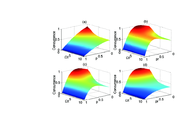
Figure 1: (Color online) The two-qubit concurrence as functions of the dimensionless quantity ${\Omega}t$ and measurement strength $p$ (or $p_{r}$) in a common photonic band gap. The parameters used here: $W_{1}=1.1$, $W_{2}=0.1$, $\Gamma_{1}=11\Omega$, $\Gamma_{2}=\Omega$ satisfy the weak-coupling regime. For the cases (a)(b) $\theta=\pi/3$, (c)(d) $\theta=\pi/6$. And (a)(c) $p_{r}=0$, i.e., only a pre weak measurement performed on the initial state, (b)(d) no pre weak measurement $p=0$, only making post-measurement (weak measurement or quantum measurement reversal) to two qubits, respectively.

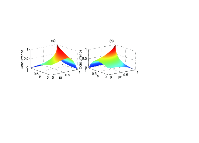
Figure 2: (Color online) The value of two-qubit entanglement trapping as functions of the pre-measurement strength $p$ and post measurement strength $p_{r}$ when the entanglement trapping occurs (here choosing $\Omega t=15$). The parameters used are: $W_{1}=1.1$, $W_{2}=0.1$, $\Gamma_{1}=11\Omega$, $\Gamma_{2}=\Omega$. For the cases (a) $\theta=\pi/3$, (b) $\theta=\pi/6$.

In Fig. 1, we show respectively the effect of the weak measurement or quantum measurement reversal on entanglement trapping of different initial states ($\theta=\pi/3$ and $\theta=\pi/6$). We demonstrate clearly that only taking the pre-measurements ($p\neq 0$, $p_{r}=0$) or the post-measurements ($p_{r}\neq 0,p=0$) to these two qubits can enhance two-qubit entanglement trapping. We note that, the edge of each graph in Fig. 1 corresponding $p=0$ or $p_{r}=0$ represents the entanglement trapping obtained without the action of any measurement. In the case $\theta=\pi/3$, the weight of $|ee\rangle$ is less than that of $|gg\rangle$ in the initial state, if we only carry out the pre-measurements on the qubits, the two-qubit entanglement trapping cannot be improved by comparing with the concurrence of entanglement trapping without introducing any operations to qubits, as shown in Fig. 1(a). While in the absence of the pre-measurement but only performing the post-measurements (quantum measurement reversal) to these two qubits respectively, the two-qubit entanglement trapping can be enhanced in a certain region of $p_{r}$, as shown in Fig. 1(b). This is because the quantum measurement reversals can decrease the $|gg\rangle$ component such that enhancement of entanglement trapping can be achieved.

In contrast, when $\theta=\pi/6$, the weight of $|ee\rangle$ is more than the weight of $|gg\rangle$, Figs. 1(c) and 1(d) reveal that two-qubit entanglement trapping can be promoted in the case of only the pre-measurements performed on the initial state within a specific $p$ range. When only post-measurements are performed to two qubits, the concurrence of entanglement trapping is smaller than that obtained without doing any operations to qubits. That means post-measurements are not necessary for this case. This is easy to understand that the pre-measurements reduce the $|ee\rangle$ component to suppress decoherence process. So two-qubit entanglement trapping can be promoted by using mainly the pre-measurements (weak measurement) to qubits when the $|ee\rangle$ weight is larger than the $|gg\rangle$ weight in the initial states. But if the $|ee\rangle$ weight is smaller than the $|gg\rangle$ weight in the initial states, quantum measurement reversals play a key role to enhance the two-qubit entanglement trapping as we mentioned previously.

Our aim is to promote the entanglement while keeping entanglement trapping by making both the pre-measurements (weak measurement) and the post-measurements (weak measurement or quantum measurement reversal). Next, we study the roles of prior weak measurement strength $p$ and post-measurement strength $p_{r}$ on concurrence of two-qubit entanglement trapping. In Figs. 2(a) and 2(b), we show the concurrence of entanglement trapping influenced by $p$ and $p_{r}$ for $\theta=\pi/3$ and $\theta=\pi/6$, and the rescaled time $\Omega t=15$ is fixed at which the phenomenon of two-qubit entanglement trapping has already occurred. From Fig. 2(a), we have verified that when the pre-measurement strength $p$ is given, the largest concurrence of entanglement trapping can be acquired through an optimal post-measurement strength $p_{r}$. And the largest concurrence and its corresponding optimal post-measurement strength $p_{r}$ both can increase with the pre weak measurement strength $p$ increasing. By contrast, in the case $\theta=\pi/6$, as shown in Fig. 2(b), the largest concurrence of entanglement trapping should relate closely with an optimal pre-measurement strength $p$ when the post-measurement strength $p_{r}$ is fixed. Moreover, the largest entanglement trapping and its corresponding optimal pre-measurement strength $p$ both can increase with the post-measurement strength $p_{r}$ increasing.

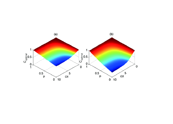
Figure 3: (Color online) The optimal concurrence of two qubits as functions of the dimensionless quantity ${\Omega}t$ and the pre-measurement strength $p$. (a) $\theta=\pi/3$, (b) $\theta=\pi/6$.

In view of the above analysis, we have two control parameters $p$ and $p_{r}$ to promote the qubits entanglement trapping. In order to obtain the most effective entanglement trapping, we note that the concurrence does not vary monotonically with $p$ for a fixed $p_{r}$, and also not vary monotonically with $p_{r}$ for a fixed $p$. Next, we investigate the optimal condition which maximizes the concurrence of entanglement trapping. By solving the extreme value of $C^{i}_{AB}(p,p_{r},t)$ in Eq.(25), the optimal post-measurement strength $p_{r}$ that gives the maximum concurrence of $\rho^{r(i)}_{AB}(p,p_{r},t)$ can be calculated as following: (i) for the case of $a(p,t)<b(p,t)$, $p_{r}$ and $p$ satisfies $p_{r}=1-\sqrt{a(p,t)/b(p,t)}$, and (ii) in the case $a(p,t)>b(p,t)$, yielding $p_{r}=1-\sqrt{b(p,t)/a(p,t)}$. Then in Figs. 3(a) and 3(b) we show the evolution of the largest concurrence of entanglement trappings $C_{optimal}$ corresponding to the above optimal conditions, depending on $p$ for $\theta=\pi/3$ and $\theta=\pi/6$. We see that the optimal entanglement trapping increase with increasing $p$ and in principle the qubits could be trapped in the maximal entanglement state if $p$ is chosen close to $1$. A comparison between Fig. 3(a) and Fig. 3(b) reveals that for different initial entanglement states, two-qubit entanglement trapping can get different promotion with an identical pre-measurement strength $p$. When the entangled state has been trapped (setting ${\Omega}t=15$), Fig. 4(a) shows the concurrence of the optimal entanglement trapping as functions of $p$ by choosing different initial states. It is clear that the concurrence of optimal entanglement trapping, which corresponds to a same $p$, increases with increasing $\theta$ in the region $\theta\in(0,\pi/2)$. However, the corresponding success probability $P_{optimal}$ decreases with the initial condition $\theta$ increasing, and also decreases monotonically with $p$ increasing, as shown in Fig. 4(b). Thus by fixing the pre-measurement strength $p$ not close to 1 for an initial entangled state, we may find the optimal promotion of entanglement trapping by our scheme with acceptable success probability $P_{optimal}$.

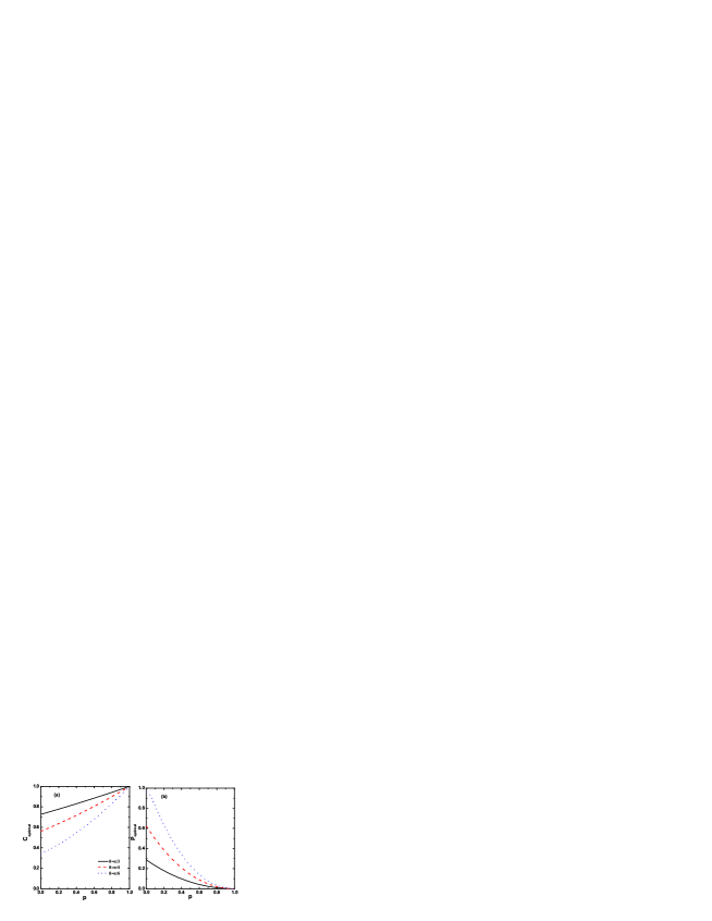
Figure 4: (Color online) The optimal concurrences $(a)$ and the corresponding success probabilities $(b)$ under our promotion scheme as functions of $p$ at different initial states when the entanglement trapping has occurred (here considering ${\Omega}t=15$). The parameters used are: $W_{1}=1.1$, $W_{2}=0.1$, $\Gamma_{1}=11\Omega$, $\Gamma_{2}=\Omega$.

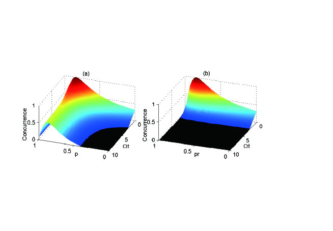
Figure 5: (Color online) The two-qubit concurrence as functions of the dimensionless quantity ${\Omega}t$ and the measurement strength $p$ (or $p_{r}$) in a common photonic band gap. The parameters used are: $\theta=\pi/20$, $W_{1}=1.1$, $W_{2}=0.1$, $\Gamma_{1}=11\Omega$, $\Gamma_{2}=\Omega$. For the cases (a) $p_{r}=0$, (b)$p=0$.

Finally, it is worth noting that ESD can also occur in the photonic band gap material when the $|ee\rangle$ weight is much larger than the $|gg\rangle$ weight. In Fig. 5, by choosing the initial state $\theta=\pi/20$, ESD appears in the case $p=p_{r}=0$ (two qubits without any measurements ). We illustrate the concurrence as functions of rescaled time $\Omega t$ and weak measurement strength $p$, as shown in Fig. 5(a). It is clear to see that ESD will never occur and entanglement trapping would appear under the condition that weak measurement strength $p$ larger than a certain value. As an example, for the parameters used in Fig. 5(a), the concurrence will never vanish when $p>0.4$. To find out the effect of the post measurement strength $p_{r}$ to ESD, we also display the evolution of two-qubit concurrence depending on $p_{r}$ in the case $p=0$ in Fig. 5(b). As can be seen, in the absence of the pre-measurements, performing the post measurements alone cannot circumvent ESD-causing. So in order to restrain ESD-causing in a photonic band gap, one should apply weak measurements with a quite large $p$, as mentioned in Ref. Kimys where two amplitude-damping decoherence channels are considered.

IV Discussion and conclusion

The entanglement trapping promotion scheme presented in this paper is valid for ideal photonic band gap. In real crystals with finite dimensions, a pseudogap corresponding to the photonic band gap can be obtained where the density of states is much smaller than that of free space, though it is not exactly zero. In these gaps, the spontaneous decay of an excited emitter is inhibited by setting its suitable position inside the photonic band gap materials Sprik ; Busch ; Woldeyohannes . This system is similar to the ideal photonic band gap for processing the scheme proposed in this paper. Hence, entanglement trapping and promotion can occur in these materials.

In our scheme, two qubits must be entangled initially in structured environments. In experiment, this initial entangled state can be generated when a pair of atoms coupled near-resonantly to the edge of photonic band gap have direct dipole-dipole interaction Nikolopoulos . Or alternatively, the entangled state for spatially separated Rydberg-atoms can be realized by choosing a three-dimensional photonic crystal single-mode cavity with high-quality $Q$ factor where atoms can freely travel through the connected void regions Guney . And in the Rydberg-atom context, by inserting a defect mode as a cavity inside the crystal, suitable atom-cavity interactions allow one to perform quantum logic gates and other cavity QED-based quantum state manipulations Guney . In other systems, for example, the coherent control of an exciton in a quantum dot is also experimentally achievable Bonadeo . Concerning about the experimental feasibility of our scheme, weak measurement and quantum measurement reversal operations for a single qubit and two qubits have already been demonstrated successfully Korotkov ; Kimys ; Katz1 ; KimYH . On the basis of the above analysis, our scheme might be implemented with current experimental technologies. In fact, the experiments are still quite challenging and there are a lot of subtle aspects to implementations.

In conclusion, we have presented the promotion entanglement trapping scheme by means of weak measurements and quantum measurement reversals. In particular, for a photonic band gap as the decoherence channel, we have shown that our protocol can enhance two-qubit entanglement trapping. We have also analyzed relationships about the optimal entanglement trapping, the corresponding success probability and weak measurement strength. Moreover, we indicate that the pre-measurement can be used to prevent ESD in the photonic band gap, comparatively the post measurements alone cannot circumvent ESD-causing. The evidences obtained show that entanglement trapping can be effectively promoted by using weak measurements and quantum measurement reversals. This highlights the potential of reservoir engineering for controlling and manipulating the dynamics of quantum systems.

V Acknowledgments

This work is supported by National Natural Science Foundation of China under Grant Nos. 11175248, 61178012, 11247240, 11304179, the Specialized Research Fund for the Doctoral Program of Higher Education under Grant Nos. 20123705120002, 20133705110001, the Provincial Natural Science Foundation of Shandong under Grant No. ZR2012FQ024, the Scientific Research Foundation of Qufu Normal University for Doctors under Grant No. BSQD20110132.

References

- (1) M. Nielsen, and I. Chuang 2000 Quantum Information and Computation (Cambridge: Cambridge University Press).
- (2) W.H. Zurek, Rev. Mod. Phys. 75 (2003) 715.
- (3) T. Yu, and J.H. Eberly, Phys. Rev. Lett.93 (2004) 140404; T. Yu, and J.H. Eberly, Science 323 (2009) 598.
- (4) M.P. Almeida, F. de Melo, M. Hor-Meyll, A. Salles, S.P. Wallborn, P.H. Souto Ribeiro, and L. Davidovich, Science 316 (2007) 579.
- (5) J. Laurat, K.S. Choi, H. Deng, C.W. Chou, and H.J. Kimble, Phys. Rev. Lett. 99 (2007) 180504.
- (6) J.S. Xu et al., Phys. Rev. Lett. 104 (2010) 100502.
- (7) Y.J. Zhang, X.B. Zou, Y.J. Xia and G.C. Guo, Phys. Rev. A 82 (2010) 022108.
- (8) J. Li and G.S. Paraoanu, New Journal of Physics 11 (2009) 113020.
- (9) C.H. Bennett, G. Brassard, S. Popescu, B. Schumacher, J.A. Smolin, and W.K. Wootters, Phys. Rev. Lett. 76 (1996) 722.
- (10) J.W. Pan, S. Gasparoni, R. Ursin, G. Weihs, and A. Zeilinger, Nature 423 (2003) 417.
- (11) R. Dong et al., Nat. Phys. 4 (2008) 919.
- (12) P. Facchi, D.A. Lidar, and S. Pascazio, Phys. Rev. A 69 (2004) 032314.
- (13) D.A. Lidar, I. Chuang, and K.B. Whaley, Phys. Rev. Lett. 81 (1998) 2594.
- (14) P.G. Kwiat, A.J. Berglund, J.B. Alterpeter and A.G. White, Science 290 (2000) 498.
- (15) S. Osnaghi, P. Bertet, A. Auffeves, P. Maioli, M. Brune, J.M. Raimond, S. Haroche, Phys. Rev. Lett. 87 (2001) 037902.
- (16) E. Hagley, X. Maitre, G. Nogues, C. Wunderlich, M. Brune, J.M. Raimond, S. Haroche, Phys. Rev. Lett. 79 (1997) 1.
- (17) M. Kon opka, V. Buek, Eur. Phys. J. D 10 (2000) 285.
- (18) Y.J. Zhang, Z.X. Man, Y.J. Xia, and G.C. Guo, Eur. Phys. J. D 58 (2010) 397.
- (19) B. Bellomo, R. Lo Franco, and G. Compagno, Advanced Science Letters 2 (2009) 459.
- (20) B. Bellomo, R. Lo Franco, S. Maniscalco, and G. Compagno, Physica Scripta T140 (2010) 014014.
- (21) C. Lazarou, K. Luoma, S. Maniscalco, J. Piilo, and B.M. Garraway, Phys. Rev. A 86 (2012) 012331.
- (22) B. Bellomo, R. Lo Franco, S. Maniscalco, and G. Compagno, Phys. Rev. A 78 (2008) 060302(R).
- (23) A.N. Korotkov and K. Keane, Phys. Rev. A 81 (2010) 040103(R).
- (24) G.S. Paraoanu, Phys. Rev. A 83 (2011) 044101.
- (25) J.C. Lee, Y.C. Jeong, Y.S. Kim, and Y.H. Kim, Opt. Express 19 (2011) 16309.
- (26) Y.S. Kim, J.C. Lee, O. Kwon, and Y.H. Kim, Nat. Phys. 8 (2012) 117.
- (27) Z.X. Man, Y.J. Xia, and N.B. An, Phys. Rev. A 86 (2012) 012325.
- (28) A.N. Korotkov, Phys. Rev. B 60 (1999) 5737.
- (29) N. Katz, et al., Phys. Rev. Lett. 101 (2008) 200401.
- (30) A.N. Korotkov, and A.N. Jordan, Phys. Rev. Lett. 97 (2006) 166805.
- (31) Y.S. Kim, Y.W. Cho, Y.S. Ra, and Y.H. Kim, Opt. Express 17 (2009) 11978.
- (32) B.M. Garraway, Phys. Rev. A 55 (1997) 2290.
- (33) B.M. Garraway, Phys. Rev. A 55 (1997) 4636.
- (34) L. Mazzola, S. Maniscalco, J. Piilo, K.-A. Suominen, and B.M. Garraway, Phys. Rev. A 79 (2009) 042302 ; 80 (2009) 012104.
- (35) W.K. Wootters, Phys. Rev. Lett. 80 (1998) 2245.
- (36) T. Yu, and J.H. Eberly, Quant. Inform. Comput. 7 (2007) 459.
- (37) H. Heydari, Quant. Inform. Comput. 6 (2006) 166.
- (38) R. Sprik, B.A. van Tiggelen, and A. Lagendijk, Europhys. Lett. 35 (1996) 265.
- (39) K. Busch, and S. John, Phys. Rev. E 58 (1998) 3896.
- (40) M. Woldeyohannes, and S. John, Phys. Rev. A 60 (1999) 5046.
- (41) G.M. Nikolopoulos, and P. Lambropoulos, J. Mod. Opt. 49 (2002) 61.
- (42) D.O. Guney, and D.A. Meyer, J. Opt. Soc. Am. B 24 (2007) 283.
- (43) N.H. Bonadeo et al., Science 282 (1998) 1473.