Dynamic Structural Equation Models for
Social Network Topology Inference^†

Abstract

Many real-world processes evolve in cascades over complex networks, whose topologies are often unobservable and change over time. However, the so-termed adoption times when blogs mention popular news items, individuals in a community catch an infectious disease, or consumers adopt a trendy electronics product are typically known, and are implicitly dependent on the underlying network. To infer the network topology, a dynamic structural equation model is adopted to capture the relationship between observed adoption times and the unknown edge weights. Assuming a slowly time-varying topology and leveraging the sparse connectivity inherent to social networks, edge weights are estimated by minimizing a sparsity-regularized exponentially-weighted least-squares criterion. To this end, solvers with complementary strengths are developed by leveraging (pseudo) real-time sparsity-promoting proximal gradient iterations, the improved convergence rate of accelerated variants, or reduced computational complexity of stochastic gradient descent. Numerical tests with both synthetic and real data demonstrate the effectiveness of the novel algorithms in unveiling sparse dynamically-evolving topologies, while accounting for external influences in the adoption times. Key events in the recent succession of political leadership in North Korea, explain connectivity changes observed in the associated network inferred from global cascades of online media.

I Introduction

Networks arising in natural and man-made settings provide the backbone for the propagation of contagions such as the spread of popular news stories, the adoption of buying trends among consumers, and the spread of infectious diseases [36, 11]. For example, a terrorist attack may be reported within minutes on mainstream news websites. An information cascade emerges because these websites’ readership typically includes bloggers who write about the attack as well, influencing their own readers in turn to do the same. Although the times when “nodes” get infected are often observable, the underlying network topologies over which cascades propagate are typically unknown and dynamic. Knowledge of the topology plays a crucial role for several reasons e.g., when social media advertisers select a small set of initiators so that an online campaign can go viral, or when healthcare initiatives wish to infer hidden needle-sharing networks of injecting drug users. As a general principle, network structural information can be used to predict the behavior of complex systems [16], such as the evolution and spread of information pathways in online media underlying e.g., major social movements and uprisings due to political conflicts [35].

Inference of networks using temporal traces of infection events has recently become an active area of research. According to the taxonomy in [16, Ch. 7], this can be viewed as a problem involving inference of association networks. Two other broad classes of network topology identification problems entail (individual) link prediction, or, tomographic inference. Several prior approaches postulate probabilistic models and rely on maximum likelihood estimation (MLE) to infer edge weights as pairwise transmission rates between nodes [34], [27]. However, these methods assume that the network does not change over time. A dynamic algorithm has been recently proposed to infer time-varying diffusion networks by solving an MLE problem via stochastic gradient descent iterations [35]. Although successful experiments on large-scale web data reliably uncover information pathways, the estimator in [35] does not explicitly account for edge sparsity prevalent in social and information networks. Moreover, most prior approaches only attribute node infection events to the network topology, and do not account for the influence of external sources such as a ground crew for a mainstream media website.

The propagation of a contagion is tantamount to causal effects or interactions being excerted among entities such as news portals and blogs, consumers, or people susceptible to being infected with a contagious disease. Acknowledging this viewpoint, structural equation models (SEMs) provide a general statistical modeling technique to estimate causal relationships among traits; see e.g., [15, 32]. These directional effects are often not revealed by standard linear models that leverage symmetric associations between random variables, such as those represented by covariances or correlations, [26], [12], [17], [2]. SEMs are attractive because of their simplicity and ability to capture edge directionalities. They have been widely adopted in many fields, such as economics, psychometrics [28], social sciences [13], and genetics [22, 6]. In particular, SEMs have recently been proposed for static gene regulatory network inference from gene expression data; see e.g., [6, 23] and references therein. However, SEMs have not been utilized to track the dynamics of causal effects among interacting nodes, or, to infer the topology of time-varying directed networks.

In this context, the present paper proposes a dynamic SEM to account for directed networks over which contagions propagate, and describes how node infection times depend on both topological (causal) and external influences. Topological influences are modeled in Section II as linear combinations of infection times of other nodes in the network, whose weights correspond to entries in the time-varying asymmetric adjacency matrix. Accounting for external influences is well motivated by drawing upon examples from online media, where established news websites depend more on on-site reporting than blog references. External influence data is also useful for model identifiability, since it has been shown necessary to resolve directional ambiguities [4]. Supposing the network varies slowly with time, parameters in the proposed dynamic SEM are estimated adaptively by minimizing a sparsity-promoting exponentially-weighted least-squares (LS) criterion (Section III-A). To account for the inherently sparse connectivity of social networks, an $\ell_{1}$-norm regularization term that promotes sparsity on the entries of the network adjacency matrix is incorporated in the cost function; see also [7, 18, 1, 2].

A novel algorithm to jointly track the network’s adjacency matrix and the weights capturing the level of external influences is developed in Section III-B, which minimizes the resulting non-differentiable cost function via a proximal-gradient (PG) solver; see e.g., [31, 10, 5]. The resulting dynamic iterative shrinkage-thresholding algorithm (ISTA) is provably convergent, and offers parallel, closed-form, and sparsity-promoting updates per iteration. Proximal-splitting algorithms such as ISTA have been successfully adopted for various signal processing tasks [9], and for parallel optimization [8]. Further algorithmic improvements are outlined in Section IV. These include enhancing the algorithms’ rate of convergence through Nesterov’s acceleration techniques [5, 29, 30] (Section IV-A), and also adapting it for real-time operation (Section IV-B). When minimal computational complexity is at a premium, a stochastic gradient descent (SGD) algorithm is developed in Section IV-C, which adaptively minimizes an instantaneous (noisy) approximation of the ensemble LS cost. Throughout, insightful and useful extensions to the proposed algorithms that are not fully developed due to space limitations are highlighted as remarks.

Numerical tests on synthetic network data demonstrate the superior error performance of the developed algorithms, and highlight their merits when compared to the sparsity-agnostic approach in [35] (Section V-A). Experiments in Section V-B involve real temporal traces of popular global events that propagated on news websites and blogs in 2011 [21]. Interestingly, topologies inferred from cascades associated to the meme “Kim Jong-un” exhibit an abrupt increase in the number of edges following the appointment of the new North Korean ruler.

Notation. Bold uppercase (lowercase) letters will denote matrices (column vectors), while operators $(\cdot)^{\top}$, $\lambda_{\max}(\cdot)$, and $\textrm{diag}(\cdot)$ will stand for matrix transposition, maximum eigenvalue, and diagonal matrix, respectively. The $N\times N$ identity matrix will be represented by ${\mathbf{I}}_{N}$, while $\mathbf{0}_{N}$ will denote the $N\times 1$ vector of all zeros, and $\mathbf{0}_{N\times P}:=\mathbf{0}_{N}\mathbf{0}^{\top}_{P}$. The $\ell_{p}$ and Frobenius norms will be denoted by $\|\cdot\|_{p}$, and $\|\cdot\|_{F}$, respectively.

II Network Model and Problem Statement

Consider a dynamic network with $N$ nodes observed over time intervals $t=1,\dots,T$, whose abstraction is a graph with topology described by an unknown, time-varying, and weighted adjacency matrix ${\mathbf{A}}^{t}\in\mathbb{R}^{N\times N}$. Entry $(i,j)$ of ${\mathbf{A}}^{t}$ (henceforth denoted by $a_{ij}^{t}$) is nonzero only if a directed edge connects nodes $i$ and $j$ (pointing from $j$ to $i$) during the time interval $t$, as illustrated in the $8$-node network in Fig. 1. As a result, one in general has $a_{ij}^{t}\neq a_{ji}^{t}$, i.e., matrix ${\mathbf{A}}^{t}$ is generally non-symmetric, which is suitable to model directed networks. For instance, if $i$ denotes a news blog maintained by a journalism student, whereas $j$ represents the web portal of a mainstream newspaper, then it is likely that $a_{ij}^{t}\gg a_{ji}^{t}\approx 0$ for those $t$ where $a_{ij}^{t}\neq 0$. Probably, the aforementioned directionality would have been reversed during Nov.-Dec. 2010, if $i$ instead represents the Wikileaks blog. Note that the model tacitly assumes that the network topology remains fixed during any given time interval $t$, but can change across time intervals.

Figure 1: Dynamic network observed across several time intervals. Note that few edges are added/removed in the transition from $t=1$ to $t=2$ (slowly time-varying network), and edges are depicted as undirected here for convenience.

Suppose $C$ contagions propagate over the network, and the difference between infection time of node $i$ by contagion $c$ and the earliest observation time is denoted by $y_{ic}^{t}$. In online media, $y_{ic}^{t}$ can be obtained by recording the time when website $i$ mentions news item $c$. For uninfected nodes at slot $t$, $y_{ic}^{t}$ is set to an arbitrarily large number. Assume that the susceptibility $x_{ic}$ of node $i$ to external (non-topological) infection by contagion $c$ is known and time invariant over the observation interval. In the web context, $x_{ic}$ can be set to the search engine rank of website $i$ with respect to (w.r.t.) keywords associated with $c$.

The infection time of node $i$ during interval $t$ is modeled according to the following dynamic structural equation model (SEM)

$$y_{ic}^{t}=\sum\limits_{j\neq i}a_{ij}^{t}y_{jc}^{t}+b_{ii}^{t}x_{ic}+e_{ic}^{t}$$ (1)

where $b_{ii}^{t}$ captures the time-varying level of influence of external sources, and $e_{ic}^{t}$ accounts for measurement errors and unmodeled dynamics. It follows from (1) that if $a_{ij}^{t}\neq 0$, then $y_{ic}^{t}$ is affected by the value of $y_{jc}^{t}$. Rewriting (1) for the entire network leads to the vector model

$${\mathbf{y}}_{c}^{t}={\mathbf{A}}^{t}{\mathbf{y}}_{c}^{t}+{\mathbf{B}}^{t}{\mathbf{x}}_{c}+{\mathbf{e}}_{c}^{t}$$ (2)

where the $N\times 1$ vector ${\mathbf{y}}_{c}^{t}:=\left[y_{1c}^{t},\dots,y_{Nc}^{t}\right]^{\top}$ collects the node infection times by contagion $c$ during interval $t$, and ${\mathbf{B}}^{t}:=\text{diag}(b_{11}^{t},\dots,b_{NN}^{t})$. Similarly, ${\mathbf{x}}_{c}:=\left[x_{1c},\dots,x_{Nc}\right]^{\top}$ and ${\mathbf{e}}_{c}^{t}:=\left[e_{1c}^{t},\dots,e_{Nc}^{t}\right]^{\top}$. Collecting observations for all $C$ contagions yields the dynamic matrix SEM

$${\mathbf{Y}}^{t}={\mathbf{A}}^{t}{\mathbf{Y}}^{t}+{\mathbf{B}}^{t}{\mathbf{X}}+{\mathbf{E}}^{t}$$ (3)

where ${\mathbf{Y}}^{t}:=\left[{\mathbf{y}}_{1}^{t},\dots,{\mathbf{y}}_{C}^{t}\right]$, ${\mathbf{X}}:=\left[{\mathbf{x}}_{1},\dots,{\mathbf{x}}_{C}\right]$, and ${\mathbf{E}}^{t}:=\left[{\mathbf{e}}_{1}^{t},\dots,{\mathbf{e}}_{C}^{t}\right]$ are all $N\times C$ matrices. Note that the same network topology ${\mathbf{A}}^{t}$ is adopted for all contagions, which is suitable e.g., when different information cascades are formed around a common meme or trending (news) topic in the Internet; see also the real data tests in Section V-B.

Given $\{{\mathbf{Y}}^{t}\}_{t=1}^{T}$ and ${\mathbf{X}}$, the goal is to track the underlying network topology $\{{\mathbf{A}}^{t}\}_{t=1}^{T}$ and the effect of external influences $\{{\mathbf{B}}^{t}\}_{t=1}^{T}$. To this end, the novel algorithm developed in the next section assumes slow time variation of the network topology and leverages the inherent sparsity of edges that is typical of social networks.

III Topology Tracking Algorithm

This section deals with a regularized LS approach to estimating $\{{\mathbf{A}}^{t},{\mathbf{B}}^{t}\}$ in (3). In a static setting with all measurements $\{{\mathbf{Y}}^{t}\}_{t=1}^{T}$ available, one solves the batch problem

$$\{\hat{{\mathbf{A}}},\hat{{\mathbf{B}}}\}=\underset{{\mathbf{A}},{\mathbf{B}}}{\text{arg min}} \frac{1}{2}\sum\limits_{t=1}^{T}\|{\mathbf{Y}}^{t}-{\mathbf{A}}{\mathbf{Y}}^{t}-{\mathbf{B}}{\mathbf{X}}\|_{F}^{2}+\lambda\|{\mathbf{A}}\|_{1}$$

s. to $$a_{ii}=0,\;b_{ij}=0,\;\forall i\neq j$$ (4)

where $\|{\mathbf{A}}\|_{1}:=\sum_{i,j}|a_{ij}|$ is a sparsity-promoting regularization, and $\lambda>0$ controls the sparsity level of $\hat{{\mathbf{A}}}$. Absence of a self-loop at node $i$ is enforced by the constraint $a_{ii}=0$, while having $b_{ij}=0,\;\forall i\neq j$, ensures that $\hat{{\mathbf{B}}}$ is diagonal as in (2).

Remark 1 (MLE versus LS)

If the errors $e_{ic}^{t}\sim\mathcal{N}(0,\sigma^{2})$ in (1) are modeled as independent and identically distributed (i.i.d.) Gaussian random variables, the sparsity-agnostic MLEs of the SEM parameters are obtained by solving

$$\min_{{\mathbf{A}},{\mathbf{B}}}\sum\limits_{t=1}^{T}\left[\frac{1}{2}\|{\mathbf{Y}}^{t}-{\mathbf{A}}{\mathbf{Y}}^{t}-{\mathbf{B}}{\mathbf{X}}\|_{F}^{2}+C\sigma^{2}\log|\det({\mathbf{I}}-{\mathbf{A}})|\right]$$ (5)

subject to the constraints in (III) [6]. Different from regression linear models, LS is not maximum likelihood (ML) when it comes to Gaussian SEMs. Sparsity can be accounted for in the ML formulation through $\ell_{1}$-norm regularization. Here, the LS approach is adopted because of its universal applicability beyond Gaussian models, and because MLE of SEM parameters gives rise to non-convex criteria [cf. (5)].

III-A Exponentially-weighted LS estimator

In practice, measurements are typically acquired in a sequential manner and the sheer scale of social networks calls for estimation algorithms with minimal storage requirements. Recursive solvers enabling sequential inference of the underlying network topology are thus preferred. Moreover, introducing a “forgetting factor” that assigns more weight to the most recent residuals makes it possible to track slow temporal variations of the topology. Note that the batch estimator (III) yields single estimates $\{\hat{\mathbf{A}},\hat{{\mathbf{B}}}\}$ that best fit the data $\{{\mathbf{Y}}^{t}\}_{t=1}^{T}$ and ${\mathbf{X}}$ over the whole measurement horizon $t=1,\ldots,T$, and as such (III) neglects potential network variations across time intervals.

For $t=1,\dots,T$, the sparsity-regularized exponentially-weighted LS estimator (EWLSE)

$$\{\hat{{\mathbf{A}}}^{t},\hat{{\mathbf{B}}}^{t}\}=\underset{{\mathbf{A}},{\mathbf{B}}}{\text{arg min}} \frac{1}{2}\sum\limits_{\tau=1}^{t}\beta^{t-\tau}\|{\mathbf{Y}}^{\tau}-{\mathbf{A}}{\mathbf{Y}}^{\tau}-{\mathbf{B}}{\mathbf{X}}\|_{F}^{2}$$

$$\;\;\;+\lambda_{t}\|{\mathbf{A}}\|_{1}$$

s. to $$a_{ii}=0,\;b_{ij}=0,\;\forall i\neq j$$ (6)

where $\beta\in(0,1]$ is the forgetting factor that forms estimates $\{\hat{{\mathbf{A}}}^{t},\hat{{\mathbf{B}}}^{t}\}$ using all measurements acquired until time $t$. Whenever $\beta<1$, past data are exponentially discarded thus enabling tracking of dynamic network topologies. The first summand in the cost corresponds to an exponentially-weighted moving average (EWMA) of the squared model residuals norms. The EWMA can be seen as an average modulated by a sliding window of equivalent length $1/(1-\beta)$, which clearly grows as $\beta\to 1$. In the so-termed infinite-memory setting whereby $\beta=1$, (III-A) boils down to the batch estimator (III). Notice that $\lambda_{t}$ is allowed to vary with time in order to capture the generally changing edge sparsity level. In a linear regression context, a related EWLSE was put forth in [1] for adaptive estimation of sparse signals; see also [18] for a projection-based adaptive algorithm.

Before moving on to algorithms, a couple of remarks are in order.

Remark 2 (Modeling slow network variations via sparsity)

To explicitly model slow topological variations across time intervals, a viable approach is to include an additional regularization term $\mu_{t}\|{\mathbf{A}}-\hat{{\mathbf{A}}}^{t-1}\|_{1}$ in the cost of (III-A). This way, the estimator penalizes deviations of the current topology estimate relative to its immediate predecessor $\hat{{\mathbf{A}}}^{t-1}$. Through the tuning parameter $\mu_{t}$, one can adjust how smooth are the admissible topology variations from interval to interval. With a similar goal but enforcing temporal smoothness via kernels with adjustable bandwidth, an $\ell_{1}$-norm-regularized logistic regression approach was put forth in [17].

Remark 3 (Selection of $\lambda_{t}$)

Selection of the (possibly time-varying) tuning parameter $\lambda_{t}$ is an important aspect of regularization methods such as (III-A), because $\lambda_{t}$ controls the sparsity level of the inferred network and how its structure may change over time. For sufficiently large values of $\lambda_{t}$ one obtains the trivial solution $\hat{{\mathbf{A}}}^{t}=\mathbf{O}_{N\times N}$, while increasingly more dense graphs are obtained as $\lambda_{t}\to 0$. An increasing $\lambda_{t}$ will be required for accurate estimation over extended time-horizons, since for $\beta\approx 1$ the norm of the LS term in (III-A) grows due to noise accumulation. This way the effect of the regularization term will be downweighted unless one increases $\lambda_{t}$ at a suitable rate, for instance proportional to $\sqrt{\sigma^{2}t}$ as suggested by large deviation tail bounds when the errors are assumed $e_{ic}^{t}\sim\mathcal{N}(0,\sigma^{2})$, and the problem dimensions $N,C,T$ are sufficiently large [26, 25, 1]. In the topology tracking experiments of Section V, a time-invariant value of $\lambda$ is adopted and typically chosen via trial and error to optimize the performance. This is justified since smaller values of $\beta$ are selected for tracking network variations, which also implies that past data (and noise) are discarded faster, and the norm of the LS term in (III-A) remains almost invariant. As future research it would be interesting to delve further into the choice of $\lambda_{t}$ using model selection techniques such as cross-validation [6], Bayesian information criterion (BIC) scores [17], or the minimum description length (MDL) principle [33], and investigate how this choice relates to statistical model consistency in a dynamic setting.

III-B Proximal gradient algorithm

Exploiting the problem structure in (III-A), a proximal gradient (PG) algorithm is developed in this section to track the network topology; see [31] for a comprehensive tutorial treatment on proximal methods. PG methods have been popularized for $\ell_{1}$-norm regularized linear regression problems, through the class of iterative shrinkage-thresholding algorithms (ISTA); see e.g., [10, 39]. The main advantage of ISTA over off-the-shelf interior point methods is its computational simplicity. Iterations boil down to matrix-vector multiplications involving the regression matrix, followed by a soft-thresholding operation [14, p. 93].

In the sequel, an ISTA algorithm is developed for the sparsity regularized dynamic SEM formulation (III-A) at time $t$. Based on this module, a (pseudo) real-time algorithm for tracking the dynamically-evolving network topology over the horizon $t=1,\ldots,T$ is obtained as well. The resulting algorithm’s memory storage requirement and computational cost per data sample $\{{\mathbf{Y}}^{t},{\mathbf{X}}\}$ does not grow with $t$.

Solving (III-A) for a single time interval $t$. Introducing the optimization variable ${\mathbf{V}}:=[{\mathbf{A}}\>{\mathbf{B}}]$, observe that the gradient of $f({\mathbf{V}}):=\frac{1}{2}\sum_{\tau=1}^{t}\beta^{t-\tau}\|{\mathbf{Y}}^{\tau}-{\mathbf{A}}{\mathbf{Y}}^{\tau}-{\mathbf{B}}{\mathbf{X}}\|_{F}^{2}$ is Lipschitz continuous with a (minimum) Lipschitz constant $L_{f}=\lambda_{\max}(\sum_{\tau=1}^{t}\beta^{t-\tau}[({\mathbf{Y}}^{\tau})^{\top}\>\>({\mathbf{X}})^{\top}]^{\top}[({\mathbf{Y}}^{\tau})^{\top}\>\>({\mathbf{X}})^{\top}])$, i.e., $\|\nabla f({\mathbf{V}}_{1})-\nabla f({\mathbf{V}}_{2})\|\leq L_{f}\|{\mathbf{V}}_{1}-{\mathbf{V}}_{2}\|$, $\forall\>{\mathbf{V}}_{1},\>{\mathbf{V}}_{2}$ in the domain of $f$. The Lipschitz constant is time varying, but the dependency on $t$ is kept implicit for notational convenience. Instead of directly optimizing the cost in (III-A), PG algorithms minimize a sequence of overestimators evaluated at judiciously chosen points ${\mathbf{U}}$ (typically the current iterate, or a linear combination of the two previous iterates as discussed in Section IV-A). From the Lipschitz continuity of $\nabla f$, for any ${\mathbf{V}}$ and ${\mathbf{U}}$ in the domain of $f$, it holds that $f({\mathbf{V}})\leq Q_{f}({\mathbf{U}},{\mathbf{V}}):=f({\mathbf{U}})+\langle\nabla f({\mathbf{U}}),{\mathbf{V}}-{\mathbf{U}}\rangle+(L_{f}/2)\|{\mathbf{V}}-{\mathbf{U}}\|_{F}^{2}$. Next, define $g({\mathbf{V}}):=\lambda_{t}\|{\mathbf{A}}\|_{1}$ and form the quadratic approximation of the cost $f({\mathbf{V}})+g({\mathbf{V}})$ [cf. (III-A)] at a given point ${\mathbf{U}}$

$$Q({\mathbf{V}},{\mathbf{U}}):={} {}Q_{f}({\mathbf{V}},{\mathbf{U}})+g({\mathbf{V}})$$

$$={} {}\frac{L_{f}}{2}\|{\mathbf{V}}-{\mathbf{G}}({\mathbf{U}})\|_{F}^{2}+g({\mathbf{V}})$$

$${}+f({\mathbf{U}})-\frac{\|\nabla f({\mathbf{U}})\|_{F}^{2}}{2L_{f}}$$ (7)

where ${\mathbf{G}}({\mathbf{U}}):={\mathbf{U}}-(1/L_{f})\nabla f({\mathbf{U}})$, and clearly $f({\mathbf{V}})+g({\mathbf{V}})\leq Q({\mathbf{V}},{\mathbf{U}})$ for any ${\mathbf{V}}$ and ${\mathbf{U}}$. Note that ${\mathbf{G}}({\mathbf{U}})$ corresponds to a gradient-descent step taken from ${\mathbf{U}}$, with step-size equal to $1/L_{f}$.

With $k=1,2,\ldots$ denoting iterations, PG algorithms set ${\mathbf{U}}:={\mathbf{V}}[k-1]$ and generate the following sequence of iterates

$${\mathbf{V}}[k]{}:={} \arg\min_{\mathbf{V}}Q({\mathbf{V}},{\mathbf{V}}[k-1])$$

$${}={} \arg\min_{\mathbf{V}}\left\{\frac{L_{f}}{2}\|{\mathbf{V}}-{\mathbf{G}}({\mathbf{V}}[k-1])\|_{F}^{2}+g({\mathbf{V}})\right\}$$ (8)

where the second equality follows from the fact that the last two summands in (III-B) do not depend on ${\mathbf{V}}$. The optimization problem (III-B) is known as the proximal operator of the function $g/L_{f}$ evaluated at ${\mathbf{G}}({\mathbf{V}}[k-1])$, and is denoted as $\textrm{prox}_{g/L_{f}}({\mathbf{G}}({\mathbf{V}}[k-1]))$. Henceforth adopting the notation ${\mathbf{G}}[k-1]:={\mathbf{G}}({\mathbf{V}}[k-1])$ for convenience, the PG iterations can be compactly rewritten as

$${\mathbf{V}}[k]=\textrm{prox}_{g/L_{f}}({\mathbf{G}}[k-1]).$$ (9)

A key element to the success of PG algorithms stems from the possibility of efficiently solving the sequence of subproblems (III-B), i.e., evaluating the proximal operator. Specializing to (III-A), note that (III-B) decomposes into

$${\mathbf{A}}[k]{}:={} \arg\min_{\mathbf{A}}\left\{\frac{L_{f}}{2}\|{\mathbf{A}}-{\mathbf{G}}_{A}[k-1]\|_{F}^{2}+\lambda_{t}\|{\mathbf{A}}\|_{1}\right\}$$

$$={} \textrm{prox}_{\lambda_{t}\|\cdot\|_{1}/L_{f}}({\mathbf{G}}_{A}[k-1])$$ (10)

$${\mathbf{B}}[k]{}:={} \arg\min_{\mathbf{B}}\left\{\|{\mathbf{B}}-{\mathbf{G}}_{B}[k-1]\|_{F}^{2}\right\}={\mathbf{G}}_{B}[k-1]$$ (11)

subject to the constraints in (III-A) which so far have been left implicit, and ${\mathbf{G}}:=[{\mathbf{G}}_{A}\>{\mathbf{G}}_{B}]$. Because there is no regularization on the matrix ${\mathbf{B}}$, the corresponding update (11) boils-down to a simple gradient-descent step. Letting $\mathcal{S}_{\mu}({\mathbf{M}})$ with $(i,j)$-th entry given by $\textrm{sign}(m_{ij})\max(|m_{ij}|-\mu,0)$ denote the soft-thresholding operator, it follows that $\textrm{prox}_{\lambda_{t}\|\cdot\|_{1}/L_{f}}(\cdot)=\mathcal{S}_{\lambda_{t}/L_{f}}(\cdot)$, e.g., [10, 14]; so that

$${\mathbf{A}}[k]=\mathcal{S}_{\lambda_{t}/L_{f}}({\mathbf{G}}_{A}[k-1]).$$ (12)

What remains now is to obtain expressions for the gradient of $f({\mathbf{V}})$ with respect to ${\mathbf{A}}$ and ${\mathbf{B}}$, which are required to form the matrices ${\mathbf{G}}_{A}$ and ${\mathbf{G}}_{B}$. To this end, note that by incorporating the constraints $a_{ii}=0$ and $b_{ij}=0,\;\forall j\neq i$, $i=1,\ldots N,$ one can simplify the expression of $f({\mathbf{V}})$ as

$$f({\mathbf{V}}):=\frac{1}{2}\sum_{\tau=1}^{t}\sum_{i=1}^{N}\beta^{t-\tau}\|({\mathbf{y}}_{i}^{\tau})^{\top}-{\mathbf{a}}_{-i}^{\top}{\mathbf{Y}}_{-i}^{\tau}-b_{ii}{\mathbf{x}}_{i}^{\top}\|_{F}^{2}$$ (13)

where $({\mathbf{y}}_{i}^{\tau})^{\top}$ and ${\mathbf{x}}_{i}^{\top}$ denote the $i$-th row of ${\mathbf{Y}}^{\tau}$ and ${\mathbf{X}}$, respectively; while ${\mathbf{a}}_{-i}^{\top}$ denotes the $1\times(N-1)$ vector obtained by removing entry $i$ from the $i$-th row of ${\mathbf{A}}$, and likewise ${\mathbf{Y}}_{-i}^{\tau}$ is the $(N-1)\times C$ matrix obtained by removing row $i$ from ${\mathbf{Y}}^{\tau}$. It is apparent from (13) that $f({\mathbf{V}})$ is separable across the trimmed row vectors ${\mathbf{a}}_{-i}^{\top}$, and the scalar diagonal entries $b_{ii}$, $i=1,\ldots,N$. The sought gradients are readily obtained as

$$\nabla_{{\mathbf{a}}_{-i}}f({\mathbf{V}})={} -\sum_{\tau=1}^{t}\beta^{t-\tau}{\mathbf{Y}}_{-i}^{\tau}({\mathbf{y}}_{i}^{\tau}-({\mathbf{Y}}_{-i}^{\tau})^{\top}{\mathbf{a}}_{-i}-{\mathbf{x}}_{i}b_{ii})$$

$$\nabla_{b_{ii}}f({\mathbf{V}})={} -\sum_{\tau=1}^{t}\beta^{t-\tau}(({\mathbf{y}}_{i}^{\tau})^{\top}-{\mathbf{a}}_{-i}^{\top}{\mathbf{Y}}_{-i}^{\tau}-b_{ii}{\mathbf{x}}_{i}^{\top}){\mathbf{x}}_{i}.$$

At time interval $t$, consider the data-related EWMAs $\bm{\Sigma}^{t}:=\sum_{\tau=1}^{t}\beta^{t-\tau}{\mathbf{Y}}^{\tau}({\mathbf{Y}}^{\tau})^{\top}$, $\bm{\sigma}_{i}^{t}:=\sum_{\tau=1}^{t}\beta^{t-\tau}{\mathbf{Y}}^{\tau}{\mathbf{y}}_{i}^{\tau}$, and $\bar{{\mathbf{Y}}}^{t}:=\sum_{\tau=1}^{t}\beta^{t-\tau}{\mathbf{Y}}^{\tau}$. With these definitions, the gradient expressions for $i=1,\ldots,N$ can be compactly expressed as

$$\nabla_{{\mathbf{a}}_{-i}}f({\mathbf{V}})={} \bm{\Sigma}_{-i}^{t}{\mathbf{a}}_{-i}+\bar{{\mathbf{Y}}}^{t}_{-i}{\mathbf{x}}_{i}b_{ii}-\bm{\sigma}_{-i}^{t}$$ (14)

$$\nabla_{b_{ii}}f({\mathbf{V}})={} {\mathbf{a}}_{-i}^{\top}\bar{{\mathbf{Y}}}^{t}_{-i}{\mathbf{x}}_{i}+\frac{1-\beta^{t}}{1-\beta}b_{ii}\|{\mathbf{x}}_{i}\|_{2}^{2}-(\bar{{\mathbf{y}}}^{\tau}_{i})^{\top}{\mathbf{x}}_{i}$$ (15)

where $(\bar{{\mathbf{y}}}^{t}_{i})^{\top}$ denotes the $i$-th row of $\bar{{\mathbf{Y}}}^{t}$, $\bar{{\mathbf{Y}}}^{t}_{-i}$ is the $(N-1)\times C$ matrix obtained by removing row $i$ from $\bar{{\mathbf{Y}}}^{t}$, and $\bm{\Sigma}_{-i}^{t}$ is the $(N-1)\times(N-1)$ matrix obtained by removing the $i$-th row and $i$-th column from $\bm{\Sigma}^{t}$.

From (11)-(12) and (14)-(15), the parallel ISTA iterations

$$\nabla_{{\mathbf{a}}_{-i}}f[k]={} \bm{\Sigma}_{-i}^{t}{\mathbf{a}}_{-i}[k]+\bar{{\mathbf{Y}}}^{t}_{-i}{\mathbf{x}}_{i}b_{ii}[k]-\bm{\sigma}_{-i}^{t}$$ (16)

$$\nabla_{b_{ii}}f[k]={} {\mathbf{a}}_{-i}^{\top}[k]\bar{{\mathbf{Y}}}^{t}_{-i}{\mathbf{x}}_{i}+\frac{(1-\beta^{t})}{1-\beta}b_{ii}[k]\|{\mathbf{x}}_{i}\|_{2}^{2}-(\bar{{\mathbf{y}}}^{t}_{i})^{\top}{\mathbf{x}}_{i}$$ (17)

$${\mathbf{a}}_{-i}[k+1]={} \mathcal{S}_{\lambda_{t}/L_{f}}\left({\mathbf{a}}_{-i}[k]-(1/L_{f})\nabla_{{\mathbf{a}}_{-i}}f[k]\right)$$ (18)

$$b_{ii}[k+1]={} b_{ii}[k]-(1/L_{f})\nabla_{b_{ii}}f[k]$$ (19)

are provably convergent to the globally optimal solution $\{\hat{{\mathbf{A}}}^{t},\hat{{\mathbf{B}}}^{t}\}$ of (III-A), as per the general convergence results available for PG methods and ISTA in particular [10, 31].

Computation of the gradients in (16)-(17) requires one matrix-vector mutiplication by $\bm{\Sigma}_{-i}^{t}$ and one by $\bar{{\mathbf{Y}}}^{t}_{-i}$, in addition to three vector inner-products, plus a few (negligibly complex) scalar and vector additions. Both the update of $b_{ii}[k+1]$ as well as the soft-thresholding operation in (18) entail negligible computational complexity. All in all, the simplicity of the resulting iterations should be apparent. Per iteration, the actual rows of the adjacency matrix are obtained by zero-padding the updated ${\mathbf{a}}_{-i}[k]$, namely setting

$${\mathbf{a}}_{i}^{\top}[k]=[a_{-i,i1}[k]\ldots a_{-i,ii-1}[k]\>0\>a_{-i,ii}[k]\ldots a_{-i,iN}[k]].$$ (20)

This way, the desired SEM parameter estimates at time $t$ are given by $\hat{{\mathbf{A}}}^{t}=[{\mathbf{a}}_{1}^{\top}[k],\ldots,{\mathbf{a}}_{N}^{\top}[k]]^{\top}$ and $\hat{{\mathbf{B}}}^{t}=\textrm{diag}(b_{11}[k],\ldots,b_{NN}[k])$, for $k$ large enough so that convergence has been attained.

Remark 4 (General sparsity-promoting regularization)

Beyond $g({\mathbf{A}})=\lambda_{t}\|{\mathbf{A}}\|_{1}$, the algorithmic framework here can accommodate more general structured sparsity-promoting regularizers $\gamma({\mathbf{A}})$ as long as the resulting proximal operator $\textrm{prox}_{\gamma/L_{f}}(\cdot)$ is given in terms of scalar or (and) vector soft-thresholding operators. In addition to the $\ell_{1}$-norm (Lasso penalty), this holds e.g., for the sum of the $\ell_{2}$-norms of vectors with groups of non-overlapping entries of ${\mathbf{A}}$ (group Lasso penalty [40]), or, a linear combination of the aforementioned two – the so-termed hierarchical Lasso penalty that encourages sparsity across and within the groups defined over ${\mathbf{A}}$ [38]. These types of regularization could be useful if one e.g., has a priori knowledge that some clusters of nodes are more likely to be jointly (in)active [35].

Solving (III-A) over the entire time horizon $t=1,\ldots,T$. To track the dynamically-evolving network topology, one can go ahead and solve (III-A) sequentially for each $t=1,\ldots,T$ as data arrive, using (16)-(19). (The procedure can also be adopted in a batch setting, when all $\{{\mathbf{Y}}^{t}\}_{t=1}^{T}$ are available in memory.) Because the network is assumed to vary slowly across time intervals, it is convenient to warm-restart the ISTA iterations, that is, at time $t$ initialize $\{{\mathbf{A}}[0],{\mathbf{B}}[0]\}$ with the previous solution $\{\hat{{\mathbf{A}}}^{t-1},\hat{{\mathbf{B}}}^{t-1}\}$. Since the sought estimates are expected to be close to the initial points, one expects convergence to be attained after few iterations.

To obtain the new SEM parameter estimates via (16)-(19), it suffices to update (possibly) $\lambda_{t}$ and the Lipschitz constant $L_{f}$, as well as the data-dependent EWMAs $\bm{\Sigma}^{t}$ ($\bm{\sigma}_{i}^{t}$ is the $i$-th column of $\bm{\Sigma}^{t}$), and $\bar{{\mathbf{Y}}}^{t}$. Interestingly, the potential growing-memory problem in storing the entire history of data $\{{\mathbf{Y}}^{t}\}_{t=1}^{T}$ can be avoided by performing the recursive updates

$$\bm{\Sigma}^{t}={} \beta\bm{\Sigma}^{t-1}+{\mathbf{Y}}^{t}({{\mathbf{Y}}^{t}})^{\top}$$ (21)

$$\bar{{\mathbf{Y}}}^{t}={} \beta\bar{{\mathbf{Y}}}^{t-1}+{\mathbf{Y}}^{t}.$$ (22)

Note that the complexity in evaluating the Gram matrix ${\mathbf{Y}}^{t}({{\mathbf{Y}}^{t}})^{\top}$ dominates the per-iteration computational cost of the algorithm. To circumvent the need of recomputing the Lipschitz constant per time interval (that in this case entails finding the spectral radius of a data-dependent matrix), the step-size $1/L_{f}$ in (18)-(19) can be selected by a line search [31]. One possible choice is the backtracking step-size rule in [5], under which convergence of (14)-(19) to $\{\hat{{\mathbf{A}}}^{t},\hat{{\mathbf{B}}}^{t}\}$ can be established as well.

Algorithm 1 Pseudo real-time ISTA for topology tracking

0:  $\left\{{\mathbf{Y}}^{t}\right\}_{t=1}^{T}$, ${\mathbf{X}}$, $\beta$.

1:  Initialize $\hat{{\mathbf{A}}}^{0}=\mathbf{0}_{N\times N},\hat{{\mathbf{B}}}^{0}=\bm{\Sigma}^{0}={\mathbf{I}}_{N},\bar{{\mathbf{Y}}}^{0}=\mathbf{0}_{N\times C},\lambda_{0}$.

2:  for $t=1,\dots,T$ do

3:     Update $\lambda_{t}$, $L_{f}$ and $\bm{\Sigma}^{t}$, $\bar{{\mathbf{Y}}}^{t}$ via (21)-(22).

4:     Initialize ${\mathbf{A}}[0]=\hat{{\mathbf{A}}}^{t-1}$, ${\mathbf{B}}[0]=\hat{{\mathbf{B}}}^{t-1}$, and set $k=0$.

5:     while not converged do

6:        for $i=1\dots N$ (in parallel) do

7:           Compute $\bm{\Sigma}_{-i}^{t}$ and $\bar{{\mathbf{Y}}}_{-i}^{t}$.

8:           Form gradients at ${\mathbf{a}}_{-i}[k]$ and $b_{ii}[k]$ via (16)-(17).

9:           Update ${\mathbf{a}}_{-i}[k+1]$ via (18).

10:           Update $b_{ii}[k+1]$ via (19).

11:           Update ${\mathbf{a}}_{i}[k+1]$ via (20).

12:        end for

13:        $k=k+1$.

14:     end while

15:     return  $\hat{{\mathbf{A}}}^{t}={\mathbf{A}}[k]$, $\hat{{\mathbf{B}}}^{t}={\mathbf{B}}[k]$.

16:  end for

Algorithm 1 summarizes the steps outlined in this section for tracking the dynamic network topology, given temporal traces of infection events $\{{\mathbf{Y}}^{t}\}_{t=1}^{T}$ and susceptibilities ${\mathbf{X}}$. It is termed pseudo real-time ISTA, since in principle one needs to run multiple (inner) ISTA iterations till convergence per time interval $t=1,\ldots,T$. This will in turn incur an associated delay, that may (or may not) be tolerable depending on the specific network inference problem at hand. Nevertheless, numerical tests indicate that in practice 5-10 inner iterations suffice for convergence; see also Fig. 2 and the discussion in Section IV-B.

Remark 5 (Comparison with the ADMM in [3])

In a conference precursor to this paper [3], an alternating-direction method of multipliers (ADMM) algorithm was put forth to estimate the dynamic SEM model parameters. While the basic global structure of the algorithm in [3] is similar to Algorithm 1, ADMM is adopted (instead of ISTA) to solve (III-A) per time $t=1,\ldots,T$. To update ${\mathbf{a}}_{-i}[k+1]$, ADMM iterations require inverting the matrix $\bm{\Sigma}_{-i}^{t}+{\mathbf{I}}_{N-1}$, that could be computationally demanding for very large networks. On the other hand, Algorithm 1 is markedly simpler and more appealing for larger-scale problems.

IV Algorithmic Enhancements and Variants

This section deals with various improvements to Algorithm 1, that pertain to accelerating its rate of convergence and also adapting it for real-time operation in time-sensitive applications. In addition, a stochastic-gradient algorithm useful when minimal computational complexity is at a premium is also outlined.

IV-A Accelerated proximal gradient method and fast ISTA

In the context of sparsity-regularized inverse problems and general non-smooth optimization, there have been several recent efforts towards improving the sublinear global rate of convergence exhibited by PG algorithms such as ISTA; see e.g., [5, 29, 30] and references therein. Since for large-scale problems first-order (gradient) methods are in many cases the only admissible alternative, the goal of these works has been to retain the computational simplicity of ISTA while markedly enhancing its global rate of convergence.

Remarkable results in [30] assert that convergence speedups can be obtained through the so-termed accelerated (A)PG algorithm. Going back to the derivations in the beginning of Section IV-A, APG algorithms generate the following sequence of iterates [cf. (III-B) and (9)]

$${\mathbf{V}}[k]=\arg\min_{\mathbf{V}}Q({\mathbf{V}},{\mathbf{U}}[k-1])=\textrm{prox}_{g/L_{f}}({\mathbf{G}}({\mathbf{U}}[k-1]))$$

where

$${\mathbf{U}}[k]{}:={} {\mathbf{V}}[k-1]+\left(\frac{c[k-1]-1}{c[k]}\right)({\mathbf{V}}[k-1]-{\mathbf{V}}[k-2])$$ (23)

$$c[k]{}={} \frac{1+\sqrt{4c^{2}[k-1]+1}}{2}.$$ (24)

In words, instead of minimizing a quadratic approximation to the cost evaluated at ${\mathbf{V}}[k-1]$ as in ISTA [cf. (III-B)], the accelerated PG algorithm [a.k.a. fast (F)ISTA] utilizes a linear combination of the previous two iterates $\{{\mathbf{V}}[k-1],{\mathbf{V}}[k-2]\}$. The iteration-dependent combination weights are function of the scalar sequence (24). FISTA offers quantifiable iteration complexity, namely a (worst-case) convergence rate guarantee of $\mathcal{O}(1/\sqrt{\epsilon})$ iterations to return an $\epsilon$-optimal solution measured by its objective value (ISTA instead offers $\mathcal{O}(1/\epsilon)$) [5, 30]. Even for general (non-)smooth optimization, APG algorithms have been shown to be optimal within the class of first-order (gradient) methods, in the sense that the aforementioned worst-case convergence rate cannot be improved [29, 30].

The FISTA solver for (III-A) entails the following steps [cf. (16)-(19)]

$$\tilde{\mathbf{a}}_{-i}[k]{}:={} {\mathbf{a}}_{-i}[k]+\left(\frac{c[k-1]-1}{c[k]}\right)({\mathbf{a}}_{-i}[k]-{\mathbf{a}}_{-i}[k-1])$$ (25)

$$\tilde{b}_{ii}[k]{}:={} b_{ii}[k]+\left(\frac{c[k-1]-1}{c[k]}\right)(b_{ii}[k]-b_{ii}[k-1])$$ (26)

$$\nabla_{{\mathbf{a}}_{-i}}f[k]={} \bm{\Sigma}_{-i}^{t}\tilde{\mathbf{a}}_{-i}[k]+\bar{{\mathbf{Y}}}^{t}_{-i}{\mathbf{x}}_{i}\tilde{b}_{ii}[k]-\bm{\sigma}_{-i}^{t}$$ (27)

$$\nabla_{b_{ii}}f[k]={} \tilde{\mathbf{a}}_{-i}^{\top}[k]\bar{{\mathbf{Y}}}^{t}_{-i}{\mathbf{x}}_{i}+\frac{(1-\beta^{t})}{1-\beta}\tilde{b}_{ii}[k]\|{\mathbf{x}}_{i}\|_{2}^{2}-(\bar{{\mathbf{y}}}^{t}_{i})^{\top}{\mathbf{x}}_{i}$$ (28)

$${\mathbf{a}}_{-i}[k+1]={} \mathcal{S}_{\lambda_{t}/L_{f}}\left(\tilde{\mathbf{a}}_{-i}[k]-(1/L_{f})\nabla_{\tilde{\mathbf{a}}_{-i}}f[k]\right)$$ (29)

$$b_{ii}[k+1]={} \tilde{b}_{ii}[k]-(1/L_{f})\nabla_{\tilde{b}_{ii}}f[k]$$ (30)

where $c[k]$ is updated as in (24). The overall (pseudo) real-time FISTA for tracking the network topology is tabulated under Algorithm 2. As desired, the computational complexity of Algorithms 1 and 2 is roughly the same. Relative to Algorithm 1, the memory requirements are essentially doubled since one now has to store the two prior estimates of ${\mathbf{A}}$ and ${\mathbf{B}}$, which are nevertheless sparse and diagonal matrices, respectively. Numerical tests in Section V suggest that Algorithm 2 exhibits the best performance when compared to Algorithm 1 and the ADMM solver of [3], especially when modified to accommodate real-time processing requirements – the subject dealt with next.

Algorithm 2 Pseudo real-time FISTA for topology tracking

0:  $\left\{{\mathbf{Y}}^{t}\right\}_{t=1}^{T}$, ${\mathbf{X}}$, $\beta$.

1:  Initialize $\hat{{\mathbf{A}}}^{0}=\mathbf{0}_{N\times N},\hat{{\mathbf{B}}}^{0}=\bm{\Sigma}^{0}={\mathbf{I}}_{N},\bar{{\mathbf{Y}}}^{0}=\mathbf{0}_{N\times C},\lambda_{0}$.

2:  for $t=1,\dots,T$ do

3:     Update $\lambda_{t}$, $L_{f}$ and $\bm{\Sigma}^{t}$, $\bar{{\mathbf{Y}}}^{t}$ via (21)-(22).

4:     Initialize ${\mathbf{A}}[0]={\mathbf{A}}[-1]=\hat{{\mathbf{A}}}^{t-1},{\mathbf{B}}[0]={\mathbf{B}}[-1]=\hat{{\mathbf{B}}}^{t-1}$, $c[0]=c[-1]=1$, and set $k=0$.

5:     while not converged do

6:        for $i=1\dots N$ (in parallel) do

7:           Compute $\bm{\Sigma}_{-i}^{t}$ and $\bar{{\mathbf{Y}}}_{-i}^{t}$.

8:           Update $\tilde{\mathbf{a}}_{-i}[k]$ and $\tilde{b}_{ii}[k]$ via (25)-(26).

9:           Form gradients at $\tilde{\mathbf{a}}_{-i}[k]$ and $\tilde{b}_{ii}[k]$ via (27)-(28).

10:           Update ${\mathbf{a}}_{-i}[k+1]$ via (29).

11:           Update $b_{ii}[k+1]$ via (30).

12:           Update ${\mathbf{a}}_{i}[k+1]$ via (20).

13:        end for

14:        $k=k+1$.

15:        Update $c[k]$ via (24).

16:     end while

17:     return  $\hat{{\mathbf{A}}}^{t}={\mathbf{A}}[k]$, $\hat{{\mathbf{B}}}^{t}={\mathbf{B}}[k]$.

18:  end for

IV-B Inexact (F)ISTA for time-sensitive operation

Additional challenges arise with real-time data collection, where analytics must often be performed “on-the-fly” as well as without an opportunity to revisit past entries. Online operation in delay-sensitive applications may not tolerate running multiple inner (F)ISTA iterations per time interval, so that convergence is attained for each $t$ as required by Algorithms 1 and 2. This section touches upon an interesting tradeoff that emerges with time-constrained data-intensive problems, where a high-quality answer that is obtained slowly can be less useful than a medium-quality answer that is obtained quickly.

Consider for the sake of exposition a scenario where the underlying network processes are stationary, or just piecewise stationary with sufficiently long coherence time for that matter. The rationale behind the proposed real-time algorithm hinges upon the fact that the solution of (III-A) for each $t=1,\ldots,T$ does not need to be super accurate in the aforementioned stationary setting, since it is just an intermediate step in the outer loop matched to the time-instants of data acquisition. This motivates stopping earlier the inner iteration which solves (III-A) (cf. the while loop in Algorithms 1 and 2), possibly even after a single soft-thresholding step, as detailed in the real-time Algorithm 3. Note that in this case the inner-iteration index $k$ coincides with the time index $t$. A similar adjustment can be made to the ISTA variant (Algorithm 1), and one can in general adopt a less aggressive approach by allowing a few (not just one) inner-iterations per $t$.

A convergence proof of Algorithm 3 in a stationary network setting will not be provided here, and is left as a future research direction. Still, convergence will be demonstrated next with the aid of computer simulations. For the infinite-memory case [cf. $\beta=1$ in (III-A)] and the simpler ISTA counterpart of Algorithm 3 obtained when $c[t]=1,\>\forall t$, it appears possible to adapt the arguments in [24, 25] to establish that the resulting iterations converge to a minimizer of the batch problem (III). In the dynamic setting where the network is time-varying, then convergence is not expected to occur because of the continuous network fluctuations. Still, as with adaptive signal processing algorithms [37] one would like to establish that the tracking error attains a bounded steady-state. These interesting and challenging problems are subject of ongoing investigation and will be reported elsewhere.

Algorithm 3 Real-time inexact FISTA for topology tracking

0:  $\left\{{\mathbf{Y}}^{t}\right\}_{t=1}^{T}$, ${\mathbf{X}}$, $\beta$.

1:  Initialize ${\mathbf{A}}[1]={\mathbf{A}}[0]=\mathbf{0}_{N\times N},{\mathbf{B}}[1]={\mathbf{B}}[0]=\bm{\Sigma}^{0}={\mathbf{I}}_{N},\bar{{\mathbf{Y}}}^{0}=\mathbf{0}_{N\times C},c[1]=c[0]=1,\lambda_{0}$.

2:  for $t=1,\dots,T$ do

3:     Update $\lambda_{t}$, $L_{f}$ and $\bm{\Sigma}^{t}$, $\bar{{\mathbf{Y}}}^{t}$ via (21)-(22).

4:     for $i=1\dots N$ (in parallel) do

5:        Compute $\bm{\Sigma}_{-i}^{t}$ and $\bar{{\mathbf{Y}}}_{-i}^{t}$.

6:        Update $\tilde{\mathbf{a}}_{-i}[t]$ and $\tilde{b}_{ii}[t]$ via (25)-(26).

7:        Form gradients at $\tilde{\mathbf{a}}_{-i}[t]$ and $\tilde{b}_{ii}[t]$ via (27)-(28).

8:        Update ${\mathbf{a}}_{-i}[t+1]$ via (29).

9:        Update $b_{ii}[t+1]$ via (30).

10:        Update ${\mathbf{a}}_{i}[t+1]$ via (20).

11:     end for

12:     Update $c[t+1]$ via (24).

13:     return  $\hat{{\mathbf{A}}}^{t}={\mathbf{A}}[t+1],\hat{{\mathbf{B}}}^{t}={\mathbf{B}}[t+1]$.

14:  end for

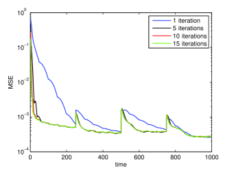
For synthetically-generated data according to the setup described in Section V-A, Fig. 2 shows the time evolution of Algorithm 2’s mean-square error (MSE) estimation performance. For each time interval $t$, (III-A) is solved “inexactly” after running only $k=1,5,10$ and $15$ inner iterations. Note that the case $k=1$ corresponds to Algorithm 3. Certainly $k=10$ iterations suffice for the FISTA algorithm to converge to the minimizer of (III-A); the curve for $k=15$ is identical. Even with $k=5$ the obtained performance is satisfactory for all practical purposes, especially after a short transient where the warm-restarts offer increasingly better initializations. While Algorithm 3 shows a desirable convergent behavior, it seems that this example’s network coherence time of $t=250$ time intervals is too short to be tracked effectively. Still, if the network changes are sufficiently smooth as it occurs at $t=750$, then the real-time algorithm is able to estimate the network reliably.

Figure 2: MSE (i.e., $\sum_{i,j}(\hat{a}_{ij}^{t}-a_{ij}^{t})^{2}/N^{2}$) performance of Algorithm 2 versus time. For each $t$, problem (III-A) is solved “inexactly” for $k=1$ (Algorithm 3), $5$, $10$, and $15$ inner iterations. It is apparent that $k=5$ iterations suffice to attain convergence to the minimizer of $\eqref{eq:ta2}$ per $t$, especially after a short transient where the warm-restarts offer increasingly better initializations.

IV-C Stochastic-gradient descent algorithm

A stochastic gradient descent (SGD) algorithm is developed in this section, which operates in real time and can track the (slowly-varying) underlying network topology. Among all algorithms developed so far, the SGD iterations incur the least computational cost.

Towards obtaining the SGD algorithm, consider $\beta=0$ in (III-A). The resulting cost function can be expressed as $f_{t}({\mathbf{V}})+g({\mathbf{V}})$, where ${\mathbf{V}}:=[{\mathbf{A}}\>{\mathbf{B}}]$ and $f_{t}({\mathbf{V}}):=(1/2)\|{\mathbf{Y}}^{t}-{\mathbf{A}}{\mathbf{Y}}^{t}-{\mathbf{B}}{\mathbf{X}}\|_{F}^{2}$ only accounts for the data acquired at time interval $t$. Motivated by computational simplicity, the “inexact” gradient descent plus soft-thresholding ISTA iterations yield the following updates

$$\nabla_{{\mathbf{a}}_{-i}}f_{t}[t]={} {\mathbf{Y}}_{-i}^{t}\left(({\mathbf{Y}}_{-i}^{t})^{\top}{\mathbf{a}}_{-i}[t]+{\mathbf{x}}_{i}b_{ii}[t]-{\mathbf{y}}_{i}^{t}\right)$$ (31)

$$\nabla_{b_{ii}}f_{t}[t]={} {\mathbf{a}}_{-i}^{\top}[t]{\mathbf{Y}}_{-i}^{t}{\mathbf{x}}_{i}+b_{ii}[t]\|{\mathbf{x}}_{i}\|^{2}-({\mathbf{y}}_{i}^{t})^{\top}{\mathbf{x}}_{i}$$ (32)

$${\mathbf{a}}_{-i}[t+1]={} \mathcal{S}_{\lambda_{t}/\eta}\left({\mathbf{a}}_{-i}[t]-\eta\nabla_{{\mathbf{a}}_{-i}}f_{t}[t]\right)$$ (33)

$$b_{ii}[t+1]={} b_{ii}[t]-\eta\nabla_{b_{ii}}f_{t}[t].$$ (34)

Compared to the parallel ISTA iterations in Algorithm 1 [cf. (16)-(18)], three main differences are noteworthy: (i) iterations $k$ are merged with the time intervals $t$ of data acquisition; (ii) the stochastic gradients $\nabla_{{\mathbf{a}}_{-i}}f_{t}[t]$ and $\nabla_{b_{ii}}f_{t}[t]$ involve the (noisy) data $\{{\mathbf{Y}}^{t}({{\mathbf{Y}}^{t}})^{\top},{\mathbf{Y}}^{t}\}$ instead of their time-averaged counterparts $\{\bm{\Sigma}^{t},\bar{{\mathbf{Y}}}^{t}\}$; and (iii) a generic constant step-size $\eta$ is utilized for the gradient descent steps.

Algorithm 4 SGD algorithm for topology tracking

0:  $\left\{{\mathbf{Y}}^{t}\right\}_{t=1}^{T}$, ${\mathbf{X}}$, $\eta$.

1:  Initialize ${\mathbf{A}}[1]=\mathbf{0}_{N\times N},{\mathbf{B}}[1]={\mathbf{I}}_{N},\lambda_{1}$.

2:  for $t=1,\dots,T$ do

3:     Update $\lambda_{t}$.

4:     for $i=1\dots N$ (in parallel) do

5:        Form gradients at ${\mathbf{a}}_{-i}[t]$ and $b_{ii}[t]$ via (31)-(32).

6:        Update ${\mathbf{a}}_{-i}[t+1]$ via (33).

7:        Update $b_{ii}[t+1]$ via (34).

8:        Update ${\mathbf{a}}_{i}[t+1]$ via (20).

9:     end for

10:     return  $\hat{{\mathbf{A}}}^{t}={\mathbf{A}}[t+1],\hat{{\mathbf{B}}}^{t}={\mathbf{B}}[t+1]$.

11:  end for

The overall SGD algorithm is tabulated under Algorithm 4. Forming the gradients in (31)-(32) requires one matrix-vector mutiplication by $({\mathbf{Y}}^{t}_{-i})^{\top}$ and two by ${\mathbf{Y}}^{t}_{-i}$. These multiplications dominate the per-iteration computational complexity of Algorithm 4, justifying its promised simplicity. Accelerated versions could be developed as well, at the expense of marginal increase in computational complexity and doubling the memory requirements.

To gain further intuition on the SGD algorithm developed, consider the online learning paradigm under which the network topology inference problem is to minimize the expected cost $E[f_{t}({\mathbf{V}})+g({\mathbf{V}})]$ (subject to the usual constraints on ${\mathbf{V}}=[{\mathbf{A}}\>{\mathbf{B}}]$). The expectation is taken w.r.t. the unknown probability distribution of the data. In lieu of the expectation, the approach taken throughout this paper is to minimize the empirical cost $C^{T}({\mathbf{V}}):=(1/T)[\sum_{t=1}^{T}f_{t}({\mathbf{V}})+g({\mathbf{V}})]$. Note that for $\beta=1$, the minimizers of $C^{T}({\mathbf{V}})$ coincide with (III) since the scaling by $1/T$ does not affect the optimal solution. For $\beta<1$, the cost $C_{\beta}^{T}({\mathbf{V}}):=\sum_{t=1}^{T}\beta^{T-t}f_{t}({\mathbf{V}})+g({\mathbf{V}})$ implements an EWMA which “forgets” past data and allows tracking. In all cases, the rationale is that by virtue of the law of large numbers, if data $\{{\mathbf{Y}}^{t}\}_{t=1}^{T}$ are stationary, solving $\lim_{T\to\infty}\min_{{\mathbf{V}}}C^{T}({\mathbf{V}})$ yields the desired solution to the expected cost.

A different approach to achieve this same goal – typically with reduced computational complexity – is to drop the expectation (or the sample averaging operator for that matter), and update the estimates via a stochastic (sub)gradient iteration ${\mathbf{V}}(t)={\mathbf{V}}(t-1)-\eta\partial\{f_{t}({\mathbf{V}})+g({\mathbf{V}})\}|_{{\mathbf{V}}={\mathbf{V}}[t-1]}$. The subgradients with respect to ${\mathbf{a}}_{-i}$ are

$$\partial_{{\mathbf{a}}_{-i}}f_{t}[t]={} {\mathbf{Y}}_{-i}^{t}\left(({\mathbf{Y}}_{-i}^{t})^{\top}{\mathbf{a}}_{-i}[t]+{\mathbf{x}}_{i}b_{ii}[t]-{\mathbf{y}}_{i}^{t}\right)$$

$$+\lambda_{t}\textrm{sign}({\mathbf{a}}_{-i}[t])$$ (35)

so the resulting algorithm has the drawback of (in general) not providing sparse solutions per iteration; see also [7] for a sparse least-mean squares (LMS) algorithm. For that reason, the approach here is to adopt the proximal gradient (ISTA) formalism to tackle the minimization of the instantaneous costs $f_{t}({\mathbf{V}})+g({\mathbf{V}})$, and yield sparsity-inducing soft-thresholded updates (33). Also acknowledging the limitation of subgradient methods to yield sparse solutions, related “truncated gradient” updates were advocated for sparse online learning in [19].

V Numerical Tests

Performance of the proposed algorithms is assessed in this section via computer simulations using both synthetically-generated network data, and real traces of information cascades collected from the web [21].

V-A Synthetic data

Data generation. Numerical tests on synthetic network data are conducted here to evaluate the tracking ability and compare Algorithms 1-4. From a “seed graph” with adjacency matrix

$$\mathbf{M}=\left(\begin{array}[]{cccc}0&0&1&1\\ 0&0&1&1\\ 0&1&0&1\\ 1&0&1&0\end{array}\right)$$

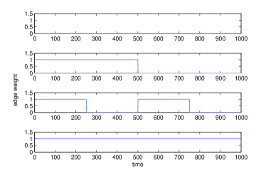
a Kronecker graph of size $N=64$ nodes was generated as described in [20]. The resulting nonzero edge weights of ${\mathbf{A}}^{t}$ were allowed to vary over $T=1,000$ intervals under $3$ settings: i) i.i.d. Bernoulli(0.5) random variables; ii) random selection of the edge-evolution pattern uniformly from a set of four smooth functions: $a_{ij}(t)=0.5+0.5\text{sin}(0.1t)$, $a_{ij}(t)=0.5+0.5\text{cos}(0.1t)$, $a_{ij}(t)=e^{-0.01t}$, and $a_{ij}(t)=0$; and iii) random selection of the edge-evolution pattern uniformly from a set of four nonsmooth functions shown in Fig. 3.

Figure 3: Nonsmooth variation of synthetically-generated edge weights of the time-varying network. For each edge, one of the four depicted profiles is chosen uniformly at random.

The number of contagions was set to $C=80$, and ${\mathbf{X}}$ was formed with i.i.d. entries uniformly distributed over $[0,3]$. Matrix ${\mathbf{B}}^{t}$ was set to $\text{diag}(\mathbf{b}^{t})$, where $\mathbf{b}^{t}\in\mathbb{R}^{N}$ is a standard Gaussian random vector. During time interval $t$, infection times were generated synthetically as ${\mathbf{Y}}^{t}=(\mathbf{I}_{N}-{\mathbf{A}}^{t})^{-1}({\mathbf{B}}^{t}{\mathbf{X}}+{\mathbf{E}}^{t})$, where ${\mathbf{E}}^{t}$ is a standard Gaussian random matrix.

Figure 4: MSE versus time obtained using pseudo real-time ISTA (Algorithm 1), for different edge evolution patterns.

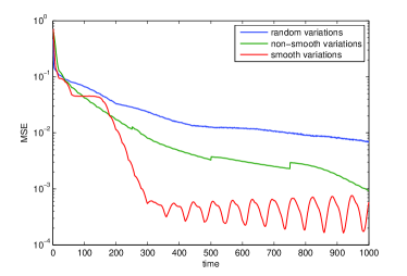
Performance evaluation. With $\beta=0.98$, Algorithm 1 was run after initializing the relevant variables as described in the algorithm table (cf. Section III-B), and setting $\lambda_{0}=25$. In addition, $\lambda_{t}=\lambda_{0}$ for $t=1,\dots,T$ as discussed in Remark 3. Fig. 4 shows the evolution of the mean-square error (MSE), $\sum_{i,j}(\hat{a}_{ij}^{t}-a_{ij}^{t})^{2}/N^{2}$. As expected, the best performance was obtained when the temporal evolution of edges followed smooth functions. Even though the Bernoulli evolution of edges resulted in the highest MSE, Algorithm 1 still tracked the underlying topology with reasonable accuracy as depicted in the heat maps of the inferred adjacency matrices; see Fig. 5.

Figure 5: Actual adjacency matrix $\hat{{\mathbf{A}}}^{t}$ and corresponding estimate $\hat{{\mathbf{A}}}^{t}$ obtained using pseudo real-time ISTA (Algorithm 1), at time intervals $t=450$ and $t=900$.

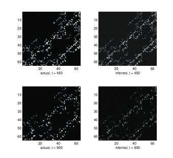
Selection of a number of parameters is critical to the performance of the developed algorithms. In order to evaluate the effect of each parameter on the network estimates, several tests were conducted by tracking the non-smooth network evolution using Algorithm 2 with varying parameter values. To illustrate the importance of leveraging sparsity of the edge weights, Fig. 6 depicts heatmaps of the adjacency matrices inferred at $t=900$, with $\lambda$ set to $0,50,$ and $100$ for all time intervals. Comparisons with the actual adjacency matrix reveal that increasing $\lambda$ progressively refines the network estimates by driving erroneously detected nonzero edge weights to $0$. Indeed, the value $\lambda=100$ in this case appears to be just about right, while smaller values markedly overestimate the support set associated with the edges present in the actual network.

Figure 6: Actual adjacency matrix at $t=900$ compared with the inferred adjacency matrices using pseudo real-time FISTA (Algorithm 2), with $\lambda_{t}=\lambda$ for all $t$ and $\lambda=0$, $\lambda=50$, and $\lambda=100$. While $\lambda=0$ and $\lambda=50$ markedly overestimate the support set associated with the true network edges, the value $\lambda=100$ in this case appears to be just about right.

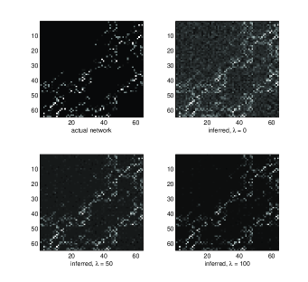
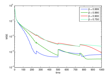
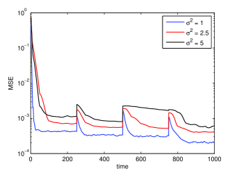
Fig. 7 compares the MSE performance of Algorithm 2 for $\beta\in\{0.999,0.990,0.900,0.750\}$. As expected, the MSE associated with values of $\beta$ approaching $1$ degrades more dramatically when changes occur within the network (at time intervals $t=250$, $t=500$, and $t=750$ in this case; see Fig. 3). The MSE spikes observed when $\beta\in\{0.999,0.990\}$ are a manifestation of the slower rate of adaptation of the algorithm for these values of the forgetting factor. In this experiment, $\beta=0.990$ outperformed the rest for $t>500$. In addition, comparisons of the MSE performance in the presence of increasing noise variance are depicted in Figure 8. Although the MSE values are comparable during the initial stages of the topology inference process, as expected higher noise levels lead to MSE performance degradation in the long run.

Figure 7: MSE performance of the pseudo real-time FISTA (Algorithm 2) versus time, for different values of the forgetting factor $\beta$.

Figure 8: MSE performance of the pseudo real-time FISTA (Algorithm 2) versus time, for different values of the noise variance $\sigma^{2}$.

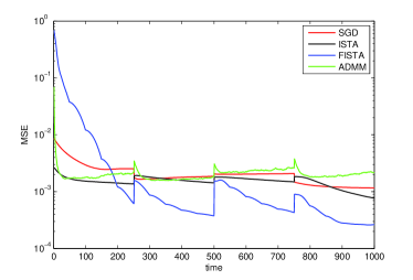
Finally, a comparison of the real-time version of the different algorithms was carried out when tracking the synthetic time-varying network with non-smooth edge variations. Specifically, the real-time (inexact) counterparts of ISTA, FISTA (cf. Algorithm 3), SGD (cf. Algorithm 4), and a suitably modified version of the ADMM algorithm developed in [3] were run as suggested in Section IV-B, i.e., eliminating the inner while loop in Algorithms 1 and 2 so that a single iteration is run per time interval. Fig. 9 compares the resulting MSE curves as the error evolves with time, showing that the inexact online FISTA algorithm achieves the best error performance. The MSE performance degradation of Algorithm 3 relative to its (exact) counterpart Algorithm 2 is depicted in Fig. 2, as a function of the number of inner iterations $k$.

Figure 9: MSE performance of the real-time algorithms versus time. Algorithms 3 (real-time FISTA) and 4 (SGD), as well as inexact versions of Algorithm 1 (ISTA) and the ADMM solver in [3] are compared.

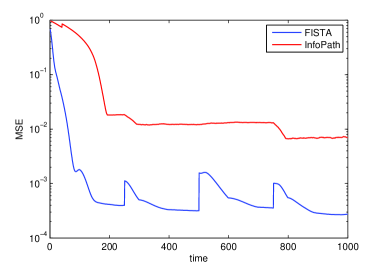
Comparison with [35]. The proposed Algorithm 2 is compared here to the method of [35], which does not explicitly account for external influences and edge sparsity. To this end, the stochastic-gradient descent algorithm (a.k.a. “InfoPath”) developed in [35] is run using the generated synthetic data with non-smooth edge variations. Postulating an exponential transmission model, the dynamic network is tracked by InfoPath by performing MLE of the edge transmission rates (see [35] for details of the model and the algorithm). Note that the postulated model therein differs from (3), used here to generate the network data. Fig. 10 depicts the MSE performance of “InfoPath” compared against FISTA. Apparently, there is an order of magnitude reduction in MSE by explicitly modeling external sources of influence and leveraging the attribute of sparsity.

Figure 10: MSE performance evolution of the pseudo real-time FISTA (Algorithm 2) compared with the InfoPath algorithm in [35].

V-B Real data

Dataset description. The real data used was collected during a prior study by monitoring blog posts and news articles for memes (popular textual phrases) appearing within a set of over $3.3$ million websites [35]. Traces of information cascades were recorded over a period of one year, from March $2011$ till February $2012$; the data is publicly available from [21]. The time when each website mentioned a specific news item was recorded as a Unix timestamp in hours (i.e., the number of hours since midnight on January $1$, $1970$). Specific globally-popular topics during this period were identified and cascade data for the top $5,000$ websites that mentioned memes associated with them were retained. The real-data tests that follow focus on the topic “Kim Jong-un”, the current leader of North Korea whose popularity rose after the death of his father and predecessor, during the observation period.

Data was first pre-processed and filtered so that only (significant) cascades that propagated to at least $7$ websites were retained. This reduced the dataset significantly to the $360$ most relevant websites over which $466$ cascades related to “Kim Jong-un” propagated. The observation period was then split into $T=45$ weeks, and each time interval was set to one week. In addition, the observation time-scale was adjusted to start at the beginning of the earliest cascade.

Matrix ${\mathbf{Y}}^{t}$ was constructed by setting $y_{ic}^{t}$ to the time when website $i$ mentioned phrase $c$ if this occurred during the span of week $t$. Otherwise $y_{ic}^{t}$ was set to a large number, $100t_{\text{max}}$, where $t_{\text{max}}$ denotes the largest timestamp in the dataset. Typically the entries of matrix ${\mathbf{X}}$ capture prior knowledge about the susceptibility of each node to each contagion. For instance, the entry ${\mathbf{x}}_{ic}$ could denote the online search rank of website $i$ for a search keyword associated with contagion $c$. In the absence of such real data, the entries of ${\mathbf{X}}$ were generated randomly from a uniform distribution over the interval $[0,0.01]$.

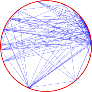
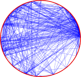
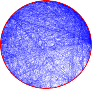
Experimental results. Algorithm 2 was run on real data with $\beta=0.9$ and $\lambda_{t}=100$. Fig. 12 depicts circular drawings of the inferred network at $t=10$, $t=30$, and $t=40$ weeks. Little was known about Kim Jong-un during the first $10$ weeks of the observation period. However, speculation about the possible successor of the dying North Korean ruler, Kim Jong-il, rose until his death on December 17, 2011 (week $38$). He was succeeded by Kim Jong-un on December 30, 2011 (week $40$). The network visualizations show an increasing number of edges over the $45$ weeks, illustrating the growing interest of international news websites and blogs in the new ruler. Unfortunately, the observation horizon does not go beyond $T=45$ weeks. A longer span of data would have been useful to investigate at what rate did the global news coverage on the topic eventually subside.

Figure 11: Plot of total number of inferred edges per week.

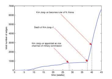
Fig. 11 depicts the time evolution of the total number of edges in the inferred dynamic network. Of particular interest are the weeks during which: i) Kim Jong-un was appointed as the vice chairman of the North Korean military commission; ii) Kim Jong-il died; and iii) Kim Jong-un became the ruler of North Korea. These events were the topics of many online news articles and political blogs, an observation that is reinforced by the experimental results shown in the plot.

(a) $t=10$

(b) $t=30$

(c) $t=40$

Figure 12: Visualization of the estimated networks obtained by tracking those information cascades related to the topic “Kim Jong-un”. The abrupt increase in network connectivity can be explained by three key events: i) Kim Jong-un was appointed as the vice chairman of the North Korean military commission ($t=28$); ii) Kim Jong-il died ($t=38$); and iii) Kim Jong-un became the ruler of North Korea ($t=40$).

VI Concluding Summary

A dynamic SEM was proposed in this paper for network topology inference, using timestamp data for propagation of contagions typically observed in social networks. The model explicitly captures both topological influences and external sources of information diffusion over the unknown network. Exploiting the inherent edge sparsity typical of large networks, a computationally-efficient proximal gradient algorithm with well-appreciated convergence properties was developed to minimize a suitable sparsity-regularized exponentially-weighted LS estimator. Algorithmic enhancements were proposed, that pertain to accelerating convergence and performing the network topology inference task in real time. In addition, reduced-complexity stochastic-gradient iterations were outlined and showed to attain worthwhile performance.

A number of experiments conducted on synthetically-generated data demonstrated the effectiveness of the proposed algorithms in tracking dynamic and sparse networks. Comparisons with the InfoPath algorithm revealed a marked improvement in MSE performance attributed to the explicit modeling of external influences and leveraging edge sparsity. Experimental results on a real dataset focused on the current ruler of North Korea successfully showed a sharp increase in the number of edges between media websites in agreement with the increased media frenzy following his ascent to power in 2011.

The present work opens up multiple directions for exciting follow-up work. Future and ongoing research includes: i) investigating the conditions for identifiability of sparse and dynamic SEMs, as well as their statistical consistency properties tied to the selection of $\lambda_{t}$; ii) formally establishing the convergence of the (inexact) real-time algorithms in a stationary network setting, and tracking their MSE performance under simple models capturing the network variation; iii) devising algorithms for MLE of dynamic SEMs and comparing the performance of the LS alternative of this paper; iii) generalizing the SEM using kernels or suitable graph similarity measures to enable network topology forecasting; and iv) exploiting the parallel structure of the algorithms to devise MapReduce/Hadoop implementations scalable to million-node graphs.

References

- [1] D. Angelosante, J. A. Bazerque, and G. B. Giannakis, “Online adaptive estimation of sparse signals: where RLS meets the -norm,” IEEE Trans. Signal Process., vol. 58, pp. 3436–3447, Jul. 2010.
- [2] D. Angelosante and G. B. Giannakis, “Sparse graphical modeling of piecewise-stationary time series,” in Proc. of Intern. Conf. on Acoustics, Speech and Signal Processing, Prague, Czech Republic, May 2011.
- [3] B. Baingana, G. Mateos, and G. B. Giannakis, “Dynamic structural equation models for tracking topologies of social networks,” in Proc. of 5th Intern. Workshop on Computational Advances in Multi-Sensor Adaptive Processing, Saint Martin, Dec. 2013.
- [4] J. A. Bazerque, B. Baingana, and G. B. Giannakis, “Identifiability of sparse structural equation models for directed and cyclic networks,” in Proc. of Global Conf. on Signal and Info. Processing, Austin, TX, Dec. 2013.
- [5] A. Beck and M. Teboulle, “A fast iterative shrinkage-thresholding algorithm for linear inverse problems,” SIAM J. Imag. Sci., vol. 2, pp. 183–202, Jan. 2009.
- [6] X. Cai, J. A. Bazerque, and G. B. Giannakis, “Gene network inference via sparse structural equation modeling with genetic perturbations,” PLoS Comp. Biology, vol. 9, May 2013, e1003068 doi:10.1371/journal.pcbi.1003068.
- [7] Y. Chen, Y. Gu, and A. O. Hero III, “Sparse LMS for system identification,” in Proc. of Intern. Conf. on Acoustics, Speech and Signal Processing, Taipei, Taiwan, Apr. 2009.
- [8] P. L. Combettes and J.-C. Pesquet, “A proximal decomposition method for solving convex variational inverse problems,” Inverse Problems, vol. 24, no. 6, pp. 1–27, 2008.
- [9] ——, “Proximal splitting methods in signal processing,” in Fixed-Point Algorithms for Inverse Problems in Science and Engineering, ser. Springer Optimization and its Applications, H. H. Bauschke, R. S. Burachik, P. L. Combettes, V. Elser, D. R. Luke, and H. Wolkowicz, Eds. Springer New York, 2011, pp. 185–212.
- [10] I. Daubechies, M. Defrise, and C. D. Mol, “An iterative thresholding algorithm for linear inverse problems with a sparsity constraint,” Comm. Pure Appl. Math., vol. 57, pp. 1413–1457, Aug. 2004.
- [11] D. Easley and J. Kleinberg, Networks, Crowds, and Markets: Reasoning About a Highly Connected World. New York, NY: Cambridge University Press, 2010.
- [12] J. Friedman, T. Hastie, and R. Tibshirani, “Sparse inverse covariance estimation with the graphical lasso,” Biostatistics, vol. 9, pp. 432–441, Dec. 2007.
- [13] A. S. Goldberger, “Structural equation methods in the social sciences,” Econometrica, vol. 40, pp. 979–1001, Nov. 1972.
- [14] T. Hastie, R. Tibshirani, and J. Friedman, The Elements of Statistical Learning, 2nd ed. Springer, 2009.
- [15] D. Kaplan, Structural Equation Modeling: Foundations and Extensions, 2nd ed. Sage Publications, 2009.
- [16] E. D. Kolaczyk, Statistical Analysis of Network Data: Methods and Models. New York, NY: Springer, 2009.
- [17] M. Kolar, L. Song, A. Ahmed, and E. P. Xing, “Estimating time-varying networks,” Ann. Appl. Statist., vol. 4, pp. 94–123, 2010.
- [18] Y. Kopsinis, K. Slavakis, and S. Theodoridis, “Online sparse system identification and signal reconstruction using projections onto weighted balls,” IEEE Trans. Signal Process., vol. 59, pp. 936–952, Mar. 2011.
- [19] J. Langford, L. Li, and T. Zhang, “Sparse online learning via truncated gradient,” J. of Machine Learning Research, vol. 10, pp. 719–743, Mar. 2009.
- [20] J. Leskovec, D. Chakrabarti, J. Kleinberg, C. Faloutsos, and Z. Ghahramani, “Kronecker graphs: An approach to modeling networks,” J. Machine Learning Research, vol. 11, pp. 985–1042, Mar. 2010.
- [21] J. Leskovec, “Web and blog datasets,” Stanford Network Analysis Project, 2011. [Online]. Available: http://snap.stanford.edu/infopath/data.html
- [22] B. Liu, A. de la Fuente, and I. Hoeschele, “Gene network inference via structural equation modeling in genetical genomics experiments,” Genetics, vol. 178, pp. 1763–1776, Mar. 2008.
- [23] B. A. Logsdon and J. Mezey, “Gene expression network reconstruction by convex feature selection when incorporating genetic perturbations,” PLoS Comp. Biology, vol. 6, Dec. 2010, e1001014. doi:10.1371/journal.pcbi.1001014.
- [24] J. Mairal, F. Bach, J. Ponce, and G. Sapiro, “Online learning for matrix factorization and sparse coding,” J. of Machine Learning Research, vol. 11, pp. 19–60, Jan. 2010.
- [25] M. Mardani, G. Mateos, and G. B. Giannakis, “Dynamic anomalography: Tracking network anomalies via sparsity and low rank,” IEEE J. Sel. Topics Signal Process., vol. 7, pp. 50–66, Feb. 2013.
- [26] N. Meinshausen and P. Buhlmann, “High-dimensional graphs and variable selection with the lasso,” Ann. Statist., vol. 34, pp. 1436–1462, 2006.
- [27] S. Meyers and J. Leskovec, “On the convexity of latent social network inference,” in Proc. of Neural Information Proc. Sys. Conf., Vancouver, Canada, Feb. 2013.
- [28] B. Muthén, “A general structural equation model with dichotomous, ordered categorical, and continuous latent variable indicators,” Pyschometrika, vol. 49, pp. 115–132, Mar. 1984.
- [29] Y. Nesterov, “A method of solving a convex programming problem with convergence rate ,” Soviet Mathematics Doklady, vol. 27, pp. 372–376, 1983.
- [30] ——, “Smooth minimization of nonsmooth functions,” Math. Prog., vol. 103, pp. 127–152, 2005.
- [31] N. Parikh and S. Boyd, “Proximal algorithms,” Found. Trends Optimization, vol. 1, pp. 123–231, 2013.
- [32] J. Pearl, Causality: Models, Reasoning, and Inference, 2nd ed. Cambridge University Press, 2009.
- [33] I. Ramirez and G. Sapiro, “An MDL framework for sparse coding and dictionary learning,” IEEE Trans. Signal Process., vol. 60, pp. 2913–2927, Jun. 2012.
- [34] M. G. Rodriguez, D. Balduzzi, and B. Scholkopf, “Uncovering the temporal dynamics of diffusion networks,” in Proc. of 28th Intern. Conf. Machine Learning, Bellevue, WA, Jul. 2011.
- [35] M. G. Rodriguez, J. Leskovec, and B. Scholkopf, “Structure and dynamics of information pathways in online media,” in Proc. of 6th ACM Intern. Conf. on Web Search and Data Mining, Rome, Italy, Dec. 2010.
- [36] E. M. Rogers, Diffusion of Innovations, 4th ed. Free Press, 1995.
- [37] V. Solo and X. Kong, Adaptive Signal Processing Algorithms: Stability and Performance. Prentice Hall, 1995.
- [38] P. Sprechmann, I. Ramirez, G. Sapiro, and Y. Eldar, “C-HiLasso: A collaborative hierarchical sparse modeling framework,” IEEE Trans. Signal Process., vol. 59, no. 9, pp. 4183–4198, Sep. 2011.
- [39] S. J. Wright, R. D. Nowak, and M. A. T. Figueiredo, “Sparse reconstruction by separable approximation,” IEEE Trans. on Sig. Proc., vol. 57, pp. 2479–2493, 2009.
- [40] M. Yuan and Y. Lin, “Model selection and estimation in regression with grouped variables,” J. Royal. Statist. Soc B, vol. 68, pp. 49–67, 2006.