The BFKL equation, Mueller-Navelet jets and single-valued harmonic polylogarithms

Abstract:

We introduce a generating function for the coefficients of the leading logarithmic BFKL Green’s function in transverse-momentum space, order by order in $\alpha_{\scriptscriptstyle S}$, in terms of single-valued harmonic polylogarithms. As an application, we exhibit fully analytic azimuthal-angle and transverse-momentum distributions for Mueller-Navelet jet cross sections at each order in $\alpha_{\scriptscriptstyle S}$. We also provide a generating function for the total cross section valid to any number of loops.

1 Introduction

In the limit in which the squared center-of-mass energy is much greater than the momentum transfer, $s\gg|t|$, any QCD scattering process is dominated by gluon exchange in the $t$ channel. Building upon this fact, the Balitsky-Fadin-Kuraev-Lipatov (BFKL) theory models strong-interaction processes with two large and disparate scales, by resumming the radiative corrections to parton-parton scattering. This is achieved to leading logarithmic accuracy, in $\ln(s/|t|)$, through the BFKL equation [1, 2, 3], i.e. an integral equation which describes the evolution of the $t$-channel gluon propagator in transverse-momentum space and Mellin moment space. The integral equation is obtained by computing the one-loop leading-logarithmic corrections to the gluon exchange in the $t$ channel. They are formed by a real correction – the emission of a gluon along the ladder [4] – and a virtual correction – the so-called one-loop Regge trajectory. The BFKL equation is then obtained by iterating these one-loop corrections to all orders in $\alpha_{\scriptscriptstyle S}$, to leading logarithmic accuracy. For $\alpha_{\scriptscriptstyle S}\ln(s/|t|)\gg 1$, one can provide an analytic solution to the BFKL equation in the saddle-point approximation [2]. The next-to-leading logarithmic (NLL) corrections to the BFKL equation are also known [5, 6, 7].

The amplitude for any QCD scattering process factorizes at leading-logarithmic accuracy into a gauge-invariant effective amplitude formed by two scattering centers, the leading order impact factors, connected by a Reggeized gluon exchanged in the crossed channel. The leading order impact factors depend on the particular scattering process. The Reggeized gluon exchange in the $t$ channel is process-independent, and it is described by the BFKL equation. Since the exchange of a gluon in the $t$ channel is required, for an arbitrary scattering the leading-order term of the BFKL resummation is often contained in the higher-order terms of the expansion in $\alpha_{\scriptscriptstyle S}$. (For example, in Drell-Yan production gluon exchange in the $t$ channel occurs at $\cal O(\alpha_{\scriptscriptstyle S}^{2})$, two orders above the leading order term of the expansion in $\alpha_{\scriptscriptstyle S}$.) For dijet production in hadron collisions, the leading order term in BFKL resummation occurs already in the leading order term of the expansion in $\alpha_{\scriptscriptstyle S}$. In this respect, dijet production in hadron collisions is the simplest process in which to consider BFKL resummation.

Long ago, Mueller and Navelet [8] suggested to look for evidence of BFKL evolution by measuring the dijet cross section at hadron colliders as a function of the hadronic centre-of-mass energy $\sqrt{S}$, at fixed momentum fractions $x_{a,b}$ of the incoming partons, and fixed minimum jet transverse momentum. This is equivalent to measuring the rates as a function of the rapidity interval $\Delta y$ between the jets. In fact, at large enough rapidities, the rapidity interval is well approximated by $\Delta y\simeq\ln(s/|t|)$, where $s=x_{a}x_{b}S$ and $|t|\simeq{p_{1}}_{{}_{\perp}}{p_{2}}_{{}_{\perp}}$, with ${p_{1}}_{{}_{\perp}}$ and ${p_{2}}_{{}_{\perp}}$ the transverse momenta of the two jets. Thus, since the cross section tends to peak at the smallest available transverse momenta, $\Delta y$ grows as $\ln S$ at fixed $x_{a,b}$. A measurement of the dijet rate at different centre-of-mass energies allows in principle for a measurement of the leading eigenvalue appearing in BFKL resummation, i.e. of the BFKL intercept. Conversely, in a fixed-energy collider, $\Delta y$ grows with $x_{a,b}$ at fixed $S$. Then evidence of the BFKL resummation may be looked for by studying dijet production cross sections at large rapidity intervals [8, 9, 10], as well as the distribution in azimuthal angle between the two jets with the largest rapidity separation [9, 10, 11, 12, 13].

The initial computations of radiative corrections to these observables were performed at leading-logarithmic (LL) accuracy in $\Delta y$. Improvements in several directions then followed, most notably in treating the BFKL resummation numerically using Monte Carlo event generators [13, 14, 15, 16], and in including the NLL BFKL corrections to dijet production [17]. A phenomenological analysis of dijet production at large $\Delta y$ at NLL accuracy can be found in ref. [18]. The dijet cross section as a function of the rapidity interval $\Delta y$ has been measured experimentally by the D0 experiment [19] at the Tevatron at different centre-of-mass energies, and by the ATLAS [20] and CMS [21] experiments at the LHC at a fixed centre-of-mass energy $\sqrt{S}=7$ TeV. The azimuthal-angle distributions of pairs of jets with wide rapidity separations have been measured by the D0 experiment [22], and quite recently by the CMS experiment [23].

In this paper, we use Mueller-Navelet jets as a template to examine the analytic dependence of the LL BFKL equation on the transverse momenta of the partons that delimit the BFKL ladder. The partons’ transverse momenta equal the transverse momenta of the two tagging jets in dijet production at large $\Delta y$. By writing the dijet cross section as an expansion in $\alpha_{\scriptscriptstyle S}\Delta y$, Mueller and Navelet were able to integrate analytically over the transverse momenta of the two tagging jets in the first few orders of the expansion. However, for the fully differential dijet cross section only a numerical solution could be provided, through either a direct integration or a Monte Carlo event generator. Recently it was found [24, 25] that the six-gluon amplitude in $\mathcal{N}=4$ super-Yang-Mills theory in multi-Regge kinematics can be described purely in terms of a class of mathematical functions known as single-valued harmonic (or multiple) polylogarithms (SVHPLs) [26]. Motivated by these developments, in this paper we use these functions to write the BFKL ladder in transverse momentum space, and thus the fully differential dijet cross section, as explicit analytic functions of the transverse momenta of the two tagging jets. More precisely, we introduce a generating function for the coefficients of the LL BFKL Green’s function, which allows us to express the Green’s function, order by order in perturbation theory, as a combination of polylogarithmic functions of one complex variable — the complexified transverse momentum — that are single-valued in the complex plane.

The paper is organized as follows: In Section 2, we recall the BFKL Green’s function and the Mueller-Navelet dijet cross section. In Section 3 we introduce our toolbox, the single-valued harmonic polylogarithms. In Section 4, we introduce a generating function for the coefficients of the BFKL Green’s function in transverse-momentum space at leading-logarithmic accuracy, and we display the coefficients explicitly up to the seventh loop. In Section 5, we sketch how our results for the BFKL Green’s function can easily be integrated over the azimuthal angle or the transverse momentum, and we provide fully analytic azimuthal-angle and transverse-momentum distributions for the Mueller-Navelet jet cross section in terms of harmonic polylogarithms up to the sixth loop, as well as a generating function for the transverse momentum distribution to any number of loops. Finally, in the same section we explicitly perform the integration of the transverse momentum distribution to obtain the total cross section, and we present a generating function for the Mueller-Navelet coefficients to any number of loops, as well as explicit results in terms of multiple zeta values up to 13 loops. In Section 6, we draw our conclusions.

2 The BFKL equation and Mueller-Navelet jets

The cross section for dijet production in the high-energy limit is dominated by gluon exchange in the crossed channel. Thus, at leading order in $\alpha_{\scriptscriptstyle S}$ the functional form of the QCD amplitudes for gluon-gluon, gluon-quark or quark-quark scattering is the same; they differ only by the color strength in the parton-production vertices. Hence the cross section takes the following factorized form,

$${d\sigma\over dp_{1_{\perp}}^{2}dp_{2_{\perp}}^{2}d\phi_{jj}dy_{1}dy_{2}}\,=\,x_{a}^{0}f_{\rm eff}(x_{a}^{0},\mu_{F}^{2})\,x_{b}^{0}f_{\rm eff}(x_{b}^{0},\mu_{F}^{2})\,{d\hat{\sigma}_{gg}\over dp_{1_{\perp}}^{2}dp_{2_{\perp}}^{2}d\phi_{jj}}\,,$$ (1)

where $1$ and $2$ label the forward and backward outgoing jets, respectively, $p_{i\bot}$ and $y_{i}$ are the jet transverse momenta and rapidities, and $\phi_{jj}$ denotes the azimuthal angle between the jets. In the high-energy limit, the parton momentum fractions are given by,

$$x_{a}^{0}=\sqrt{p_{1_{\perp}}^{2}\over S}\,e^{y_{1}}\,,\qquad\qquad x_{b}^{0}=\sqrt{p_{2_{\perp}}^{2}\over S}\,e^{-y_{2}}\,,$$ (2)

and the effective parton distribution functions are

$$f_{\rm eff}(x,\mu_{F}^{2})=G(x,\mu_{F}^{2})+{4\over 9}\sum_{f}\left[Q_{f}(x,\mu_{F}^{2})+\bar{Q}_{f}(x,\mu_{F}^{2})\right],$$ (3)

where the sum is over the quark flavors, and $\mu_{F}$ is the factorization scale.

The gluon-gluon scattering cross section in the high-energy limit becomes,

$$\frac{d\hat{\sigma}_{gg}}{dp_{1\bot}^{2}dp_{2\bot}^{2}d\phi_{jj}}=\frac{\pi}{2}\,\left[\frac{C_{A}\alpha_{\scriptscriptstyle S}}{p_{1\bot}^{2}}\right]\,f(\vec{q}_{1\bot},\vec{q}_{2\bot},\Delta y)\,\left[\frac{C_{A}\alpha_{\scriptscriptstyle S}}{p_{2\bot}^{2}}\right]\,,$$ (4)

where $\Delta y=y_{1}-y_{2}$ is the rapidity difference between the two jets. The variables $\vec{q}_{i\bot}$ that enter the Green’s function $f(\vec{q}_{1\bot},\vec{q}_{2\bot},\Delta y)$ are related to the transverse momenta of the jets by $\vec{q}_{1\bot}=-\vec{p}_{1\bot}$ and $\vec{q}_{2\bot}=\vec{p}_{2\bot}$. Fixing

$$\eta\equiv\displaystyle{\frac{C_{A}\,\alpha_{\scriptscriptstyle S}}{\pi}}\,\Delta y\,,$$ (5)

at leading logarithmic accuracy the Green’s function is given by

$$f(\vec{q}_{1\bot},\vec{q}_{2\bot},\Delta y)=\frac{1}{(2\pi)^{2}\,\sqrt{q_{1\bot}^{2}\,q_{2\bot}^{2}}}\,\sum_{n=-\infty}^{+\infty}e^{in\phi}\,\int_{-\infty}^{+\infty}d\nu\,\left(\frac{q_{1\bot}^{2}}{q_{2\bot}^{2}}\right)^{i\nu}\,e^{\eta\,\chi_{\nu,n}}\,,$$ (6)

where $q_{i\bot}^{2}=|\vec{q}_{i\bot}|^{2}$, and $\phi$ is the angle between $\vec{q}_{1\bot}$ and $\vec{q}_{2\bot}$ (and therefore $\phi=\pi-\phi_{jj}$). The exponent in eq. (6) is given by $\eta\,\chi_{\nu,n}=\Delta y\,\omega(\nu,n)$, where

$$\omega(\nu,n)=\frac{C_{A}\alpha_{\scriptscriptstyle S}}{\pi}\,\chi_{\nu,n}\,,$$ (7)

is the LL BFKL eigenvalue, with

$$\chi_{\nu,n}=-2\gamma_{E}-\psi\left(\frac{1}{2}+\frac{|n|}{2}+i\nu\right)-\psi\left(\frac{1}{2}+\frac{|n|}{2}-i\nu\right)\,.$$ (8)

2.1 The saddle-point approximation

For $\eta\gg 1$, we may perform a saddle-point approximation to the integral over $\nu$ in the gluon Green’s function (6). The saddle point is near $\nu=0$. We use the small-$\nu$ expansion of the BFKL eigenvalue, eq. (100),

$$\chi_{\nu,n}=2\left(a_{0n}+a_{1n}\nu^{2}+\cdots\right)\,,$$ (9)

with the coefficients given in eq. (105). Then we can write the gluon Green’s function (6) as,

$$f(\vec{q}_{1\bot},\vec{q}_{2\bot},\Delta y)=\frac{1}{4\pi\,\sqrt{q_{1\bot}^{2}\,q_{2\bot}^{2}}}\,\sum_{n=-\infty}^{+\infty}e^{in\phi}\,\frac{\exp\left(2a_{0n}\eta-\displaystyle\frac{\ln^{2}\frac{q_{1\bot}^{2}}{q_{2\bot}^{2}}}{4(-2a_{1n})\eta}\right)}{\sqrt{\pi(-2a_{1n})\eta}}\,.$$ (10)

Note that $a_{1n}$, as given in eq. (105), is always negative; thus the saddle-point approximation is well defined. Integrating out the azimuthal angle, which singles out the $n=0$ contribution, and using $a_{00}$ and $a_{10}$ as given in eq. (102), we obtain the usual saddle-point approximation of the BFKL Green’s function.

2.2 The azimuthal angle distribution

Integrating out the jet transverse momenta over $E_{{}_{\perp}}\leq p_{{}_{\perp}}<\infty$, eq. (4) becomes

$${d\hat{\sigma}_{gg}\over d\phi_{jj}}\ =\frac{\pi(C_{A}\alpha_{\scriptscriptstyle S})^{2}}{2E_{\bot}^{2}}\left[\delta(\phi_{jj}-\pi)+\sum_{k=1}^{\infty}\left(\sum_{n=-\infty}^{\infty}\frac{e^{in\phi}}{2\pi}f_{n,k}\right)\eta^{k}\right]\,,$$ (11)

with

$$f_{n,k}={1\over 2\pi}\,\frac{1}{k!}\,\int_{-\infty}^{\infty}d\nu\,\frac{\chi_{\nu,n}^{k}}{\nu^{2}+\frac{1}{4}}\,.$$ (12)

The Born term has been singled out by performing the integral in $f_{n,0}$, which yields $f_{n,0}=1$, and furthermore by using,

$${1\over 2\pi}\sum_{n=-\infty}^{\infty}e^{in\phi}=\delta(\phi_{jj}-\pi)\,.$$ (13)

In the limit $\alpha_{\scriptscriptstyle S}\Delta y\to 0$, eq. (11) reduces to the azimuthal distribution at leading order. Note that by using the recursive formula (98) for the $\chi_{\nu,n}$ coefficients, we can obtain a recursive formula for the Fourier coefficients $f_{n,k}$, in terms of a one-dimensional integral over $\nu$.

2.3 The Mueller-Navelet dijet cross section

When the azimuthal angle is integrated out over the full range $0\leq\phi_{jj}\leq 2\pi$, only the zero mode of eq. (11) survives,

$$\int_{0}^{2\pi}d\phi_{jj}e^{in\phi}=2\pi\delta_{n,0}\,,$$ (14)

and we obtain the Mueller-Navelet dijet cross section,

$$\hat{\sigma}_{gg}=\frac{\pi(C_{A}\alpha_{\scriptscriptstyle S})^{2}}{2E_{\bot}^{2}}\,\sum_{k=0}^{\infty}f_{0,k}\,\eta^{k}\,.$$ (15)

Mueller and Navelet [8] computed analytically the first few coefficients of the expansion (15),

$$\begin{split}f_{0,0}&\,=1\,,\\ f_{0,1}&\,=0\,,\\ f_{0,2}&\,=2\zeta_{2}\,,\\ f_{0,3}&\,=-3\zeta_{3}\,,\\ f_{0,4}&\,=\frac{53}{6}\,\zeta_{4}\,,\\ f_{0,5}&\,=-\frac{1}{12}\,(115\zeta_{5}+48\zeta_{2}\zeta_{3})\,.\end{split}$$ (16)

However, for the fully differential dijet cross section (4), so far only a numerical solution could be provided, through either a direct integration or a Monte Carlo event generator.

3 Single-valued harmonic polylogarithms

In this section we give a short review of the main tools that allow us to solve the Green’s function perturbatively, namely harmonic polylogarithms (HPLs) and their single-valued analogues. We start by reviewing the multi-valued case, and we then briefly recall the construction of the single-valued analogues of ref. [26] (see also ref. [27]).

Harmonic polylogarithms were first introduced in the physics literature in ref. [28]. They are defined iteratively through the differential equations

$$\frac{d}{dz}H_{0\,\omega}(z)=\frac{H_{\omega}(z)}{z}\quad\quad\text{and}\quad\quad\frac{d}{dz}H_{1\,\omega}(z)=\frac{H_{\omega}(z)}{1-z}\,,$$ (17)

where $\omega$ denotes any word formed out of the letters ‘0’ and ‘1’. The length $|\omega|$ of the word $\omega$ is called the weight of $H_{\omega}(z)$. The solutions of the differential equation are subject to the constraints,

$$H(z)=1,\quad\quad H_{\vec{0}_{n}}(z)=\frac{1}{n!}\ln^{n}z,\quad\quad\text{and}\quad\quad\lim_{z\rightarrow 0}H_{\omega\neq\vec{0}_{n}}(z)=0\,.$$ (18)

It is easy to check that the solutions to these differential equations are given by the iterated integrals

$$H_{a\omega}(z)=\int_{0}^{z}dt\,f_{a}(t)\,H_{\omega}(t)\,,$$ (19)

with

$$f_{0}(z)=\frac{1}{z}\quad\quad\text{and}\quad\quad f_{1}(z)=\frac{1}{1-z}\,.$$ (20)

HPLs enjoy many properties. In particular, they form a shuffle algebra, i.e.,

$$H_{\omega_{1}}(z)\,H_{\omega_{2}}(z)=\sum_{{\omega}\in{\omega_{1}}\mbox{\bf\scyr X}{\omega_{2}}}H_{\omega}(z)\,,$$ (21)

where ${\omega_{1}}{\mbox{\cyr X}}{\omega_{2}}$ is the set of mergers, or shuffles, of the sequences $\omega_{1}$ and $\omega_{2}$; each element of the set is an interleaving of the two sequences such that the orderings of the letters inside $\omega_{1}$, and of those inside $\omega_{2}$, are preserved. Furthermore, the HPLs contain the classical polylogarithms as special cases,

$$H_{\scriptsize\underbrace{0\ldots 0}_{m-1}1}(z)={\rm Li}_{m}(z)=\int_{0}^{z}dt\;\frac{{\rm Li}_{m-1}(t)}{t}\,,$$ (22)

with ${\rm Li}_{1}(z)=-\ln(1-z)$.

Due to the singularities in the differential equations (17), HPLs in general define multi-valued functions on the punctured complex plane $\mathbb{C}/\{0,1\}$. In ref. [26] it was shown that for every HPL $H_{\omega}(z)$ there is a function $\mathcal{L}_{\omega}(z)$ that is real-analytic and single-valued on $\mathbb{C}/\{0,1\}$ and that satisfies the same properties as the ordinary HPLs. That is, the $\cal L_{\omega}(z)$ satisfy the differential equations

$$\frac{\partial}{\partial z}\cal L_{0\,\omega}(z)=\frac{\cal L_{\omega}(z)}{z}\quad\quad\text{and}\quad\quad\frac{\partial}{\partial z}\cal L_{1\,\omega}(z)=\frac{\cal L_{\omega}(z)}{1-z}\,,$$ (23)

subject to the conditions

$$\cal L(z)=1\,,\quad\quad\cal L_{\vec{0}_{n}}(z)=\frac{1}{n!}\ln^{n}|z|^{2}\quad\quad\text{and}\quad\quad\lim_{z\rightarrow 0}\cal L_{\omega\neq\vec{0}_{n}}(z)=0\,.$$ (24)

In addition, the SVHPLs $\mathcal{L}_{\omega}(z)$ also form a shuffle algebra,

$$\mathcal{L}_{\omega_{1}}(z)\,\mathcal{L}_{\omega_{2}}(z)=\sum_{{\omega}\in{\omega_{1}}\mbox{\bf\scyr X}{\omega_{2}}}\mathcal{L}_{\omega}(z)\,.$$ (25)

SVHPLs can be explicitly expressed as combinations of ordinary HPLs such that all the branch cuts cancel. In order to understand how these combinations can be constructed, and also to understand the solution for the BFKL Green’s function in Section 4, it is useful to first get a new viewpoint on ordinary HPLs.

It is clear from the previous discussion that for every word $\omega$ formed out of the letters ‘0’ and ‘1’ there is a harmonic polylogarithm $H_{\omega}(z)$. Let us therefore denote the set of all words formed out of the non-commutative variables $x_{0}$ and $x_{1}$ by $X^{*}$, and let $\mathbb{C}\langle X\rangle$ be the complex vector space generated by the elements in $X^{*}$, i.e., the vector space of all formal $\mathbb{C}$-linear combinations of elements in $X^{*}$. $\mathbb{C}\langle X\rangle$ can be turned into an algebra by equipping it with the concatenation of words as multiplication. The set of differential equations (17) can then be conveniently summarized by a single differential equation for a generating function $L(z)$, often referred to as a Knizhnik-Zamolodchikov (KZ) equation [29]

$$\frac{d}{dz}L(z)=\left(\frac{x_{0}}{z}+\frac{x_{1}}{1-z}\right)\,L(z)\,,\qquad L(z)\in\mathbb{C}\langle X\rangle\,.$$ (26)

It is easy to see that a solution to the KZ equation is given by

$$L(z)=\sum_{\omega\in X^{*}}H_{\omega}(z)\,\omega\,,$$ (27)

where obviously for the empty word $e$ we have $H_{e}(z)=H(z)=1$. We can then define the single-valued analogues of the ordinary HPLs by constructing a single-valued generating-function solution

$$\mathcal{L}(z)=\sum_{\omega\in X^{*}}\mathcal{L}_{\omega}(z)\,\omega$$ (28)

of the analogous KZ equation,

$$\frac{\partial}{\partial z}\mathcal{L}(z)=\left(\frac{x_{0}}{z}+\frac{x_{1}}{1-z}\right)\,\mathcal{L}(z)\,,\qquad\mathcal{L}(z)\in\mathbb{C}\langle X\rangle\,,$$ (29)

subject to the conditions (24). We briefly review the construction of $\cal L(z)$ of ref. [26] in the rest of this section.

We start by defining a second alphabet $\{y_{0},y_{1}\}$ (and a set of words $Y^{*}$) and a map ${}^{\sim}:Y^{*}\rightarrow Y^{*}$ as the operation that reverses words. The alphabets $\{x_{0},x_{1}\}$ and $\{y_{0},y_{1}\}$ are not independent but they are related by the following relations,

$$\begin{split}y_{0}&\,=\,x_{0}\\ \tilde{Z}(y_{0},y_{1})y_{1}\tilde{Z}(y_{0},y_{1})^{-1}&\,=\,Z(x_{0},x_{1})^{-1}x_{1}Z(x_{0},x_{1})\,,\end{split}$$ (30)

where $Z(x_{0},x_{1})$ denotes the Drinfel’d associator, defined by the series,

$$Z(x_{0},x_{1})=\sum_{\omega\in X^{*}}\zeta(\omega)\omega=L(1),$$ (31)

where $\zeta(\omega)=H_{\omega}(1)$ for $\omega\neq x_{1}$ and $\zeta(x_{1})=0$. The $\zeta(\omega)$ are regularized by the shuffle algebra [30]; that is, we use the shuffle algebra to define the naively divergent cases. Using a collapsed notation for $\omega$, in which zero entries are removed according to $\vec{0}_{m-1}1\to m$, these $\zeta(\omega)$ are the familiar multiple zeta values. The inversion operator is to be understood as a formal series expansion in the weight $|\omega|$ (also known as the length of the word $\omega$).

We can solve eq. (30) iteratively in the length of the word. This yields a series expansion for $y_{1}$. Next, let $\phi:Y^{*}\rightarrow X^{*}$ be the map that renames $y$ to $x$, i.e. $\phi(y_{0})=x_{0}$ and $\phi(y_{1})=x_{1}$, define the generating functions

$$L_{X}(z)\,=\,\sum_{\omega\in X^{*}}H_{\omega}(z)\omega\,,\qquad\tilde{L}_{Y}(\bar{z})\,=\,\sum_{\omega\in Y^{*}}H_{\phi(\omega)}(\bar{z})\tilde{\omega}\,,$$ (32)

where $\bar{z}$ denotes the complex conjugate of $z$. It was shown in ref. [26] that the generating function (28) for the single-valued analogues of HPLs is then obtained by

$$\cal L(z)=\sum_{\omega\in X^{*}}\cal L_{\omega}(z)\,\omega=L_{X}(z)\,\tilde{L}_{Y}(\bar{z})\,.$$ (33)

Expanding the right-hand side of eq. (33), the coefficient of each word $\omega\in X^{*}$ is a combination of HPLs such that the branch cuts cancel, i.e. it is single-valued on $\mathbb{C}/\{0,1\}$.

4 The BFKL equation and single-valued harmonic polylogarithms

We now apply the ideas of the previous section to the BFKL Green’s function. In particular, we provide (at least conjecturally) a generating function for the coefficients appearing in the perturbative expansion of the BFKL Green’s function. The Green’s function is a function of the (two-dimensional) transverse momenta $p_{1\bot}$ and $p_{2\bot}$. For the rest of the discussion, it turns out to be convenient to encode the information on each transverse momentum by a single complex number, $p_{k\bot}\to{\tilde{p}_{k}}=p^{x}_{k}+ip^{y}_{k}$. Furthermore, we introduce a complex variable $w$ by

$$w=\frac{\tilde{p}_{1}}{\tilde{p}_{2}}{\rm~{}~{}~{}~{}and~{}~{}~{}~{}}w^{\ast}=\frac{\tilde{p}_{1}^{\ast}}{\tilde{p}_{2}^{\ast}}\,,$$ (34)

such that

$$|w|^{2}=\frac{|\tilde{p}_{1}|^{2}}{|\tilde{p}_{2}|^{2}}=\frac{p_{1\bot}^{2}}{p_{2\bot}^{2}}=\frac{q_{1\bot}^{2}}{q_{2\bot}^{2}}{\rm~{}~{}~{}~{}and~{}~{}~{}~{}}\left(\frac{w}{w^{\ast}}\right)^{1/2}=e^{-i\phi_{jj}}=-e^{i\phi}\,.$$ (35)

The Green’s function can be expanded into a power series in $\eta$,

$$f(\vec{q}_{1\bot},\vec{q}_{2\bot},\Delta y)=\frac{1}{2}\delta^{(2)}(\vec{q}_{1\bot}-\vec{q}_{2\bot})+\frac{1}{2\pi\,\sqrt{q_{1\bot}^{2}\,q_{2\bot}^{2}}}\,\sum_{k=1}^{\infty}\eta^{k}\,f_{k}(w,w^{\ast})\,,$$ (36)

where the coefficients $f_{k}$ are given by the inverse Fourier-Mellin transform,

$$f_{k}(w,w^{\ast})=\frac{1}{k!}\sum_{n=-\infty}^{+\infty}(-1)^{n}\,\left(\frac{w}{w^{\ast}}\right)^{n/2}\int_{-\infty}^{+\infty}\frac{d\nu}{2\pi}\,|w|^{2i\nu}\,\chi_{\nu,n}^{k}\,.$$ (37)

These coefficients should be real-analytic functions of $w$; that is, they should have a unique, well-defined value for every ratio of the magnitudes of the two jet transverse momenta and angle between them.

The invariance of eq. (37) under $n\leftrightarrow-n$ and $\nu\leftrightarrow-\nu$ implies that $f_{k}$ is invariant under conjugation and inversion of $w$:

$$f_{k}(w,w^{\ast})=f_{k}(w^{\ast},w)=f_{k}(1/w,1/w^{\ast})\,.$$ (38)

In other words, the perturbative coefficients are eigenfunctions under the action of the $\mathbb{Z}_{2}\times\mathbb{Z}_{2}$ symmetry generated by

$$(w,w^{\ast})\leftrightarrow(w^{\ast},w){\rm~{}~{}~{}~{}and~{}~{}~{}~{}}(w,w^{\ast})\leftrightarrow(1/w,1/w^{\ast})\,.$$ (39)

From eq. (34) we see that a special point in the $(w,w^{\ast})$ plane is at $w=w^{\ast}=-1$. This is the configuration of Born kinematics, where the two jets have equal and opposite transverse momentum. A second preferred point is the origin, $w=w^{\ast}=0$, when one jet has much smaller transverse momentum than the other jet. The point at infinity is related to the origin by the inversion symmetry, while $w=w^{\ast}=-1$ is a fixed point of the $\mathbb{Z}_{2}\times\mathbb{Z}_{2}$ symmetry (39). We anticipate that the SVHPLs $\cal L_{\omega}(z,\bar{z})$ will play a role. However, their poles are at $z=0$ and 1, not $w=0$ and $-1$, so we will need to identify $(z,\bar{z})=(-w,-w^{\ast})$.

In the rest of this section we argue that one can use SVHPLs to write down a generating function for the perturbative coefficients $f_{k}(w,w^{\ast})$ to all orders in the expansion parameter $\eta$. In order to present the generating function, we need to introduce some definitions. First, similar to the vector space $\mathbb{C}\langle X\rangle$ defined in the previous section, we define $\mathbb{C}\langle\cal L\rangle$ as the vector space generated by all SVHPLs $\cal L_{\omega}(z)\equiv\cal L_{\omega}(-w)$. Note that there is a natural linear map $\mathcal{P}_{\cal L}:\mathbb{C}\langle X\rangle\to\mathbb{C}\langle\cal L\rangle$ sending a word $\omega$ to the SVHPL $\cal L_{\omega}(z)$. In order to incorporate the expansion parameter $\eta$, we enlarge the vector space $\mathbb{C}\langle X\rangle$ to the ring $\mathbb{C}\langle X\rangle[[\eta]]$ of formal power series in $\eta$ with coefficients in $\mathbb{C}\langle X\rangle$. The ring $\mathbb{C}\langle\cal L\rangle[[\eta]]$ is defined in a similar fashion, and the map $\mathcal{P}_{\cal L}$ extends in an obvious manner to a map from $\mathbb{C}\langle X\rangle[[\eta]]$ to $\mathbb{C}\langle\cal L\rangle[[\eta]]$.

By observing patterns in the coefficients of the SVHPLs that appear at low orders in the $\eta$ expansion (see e.g. eq. (45)), and inspired by a very similar problem in $\cal N=4$ super-Yang-Mills theory [25] (see below), we have found an all-orders formula that reproduces the first 10 orders of the expansion. In order to describe this formula compactly, we define the following elements of $\mathbb{C}\langle X\rangle[[\eta]]$,

$$\begin{split}\mathcal{X}(x_{0},x_{1};\eta)&\,=\,\left[1-\left(\frac{e^{-x_{0}\eta}-1}{x_{0}}\right)x_{1}\right]^{-1}\,,\\ \cal Z(x_{0};\eta)&\,=\,\sum_{k=1}^{\infty}\left[\sum_{n=0}^{k-1}(-x_{0})^{k-n-1}\sum_{m=0}^{n}\,\frac{2^{m}}{(k-m)!}\,\mathfrak{Z}(n,m)\right]\,\eta^{k}\,,\\ \end{split}$$ (40)

where the $\mathfrak{Z}(n,m)$ are particular combinations of $\zeta$ values of uniform weight $n$. They are related to partial Bell polynomials, and are generated by the series,

$$\begin{split}\exp\left\{-\frac{x\,y}{2}\,\left[2\gamma_{E}+\psi(1+x)+\psi(1-x)\right]\right\}&\,=\exp\left[y\sum_{k=1}^{\infty}\zeta_{2k+1}x^{2k+1}\right]\\ &\,=\sum_{n=0}^{\infty}\sum_{m=0}^{\infty}\mathfrak{Z}(n,m)\,x^{n}y^{m}\,.\end{split}$$ (41)

We are now in the position to state our main conjecture: the BFKL Green’s function can be written, to all orders in the perturbative expansion parameter $\eta$, as

$$f(\vec{q}_{1\perp},\vec{q}_{2\perp},\Delta y)=\frac{1}{2}\delta^{(2)}(\vec{q}_{1\perp}-\vec{q}_{2\perp})+\frac{1}{2\pi|\vec{q}_{1\perp}-\vec{q}_{2\perp}|^{2}}\,\mathcal{P}_{\cal L}\left[\mathcal{X}(x_{0},x_{1};\eta)\,\cal Z(x_{0};\eta)\right]\,.$$ (42)

Equation (42) can be interpreted as a generating function for the perturbative coefficients $f_{k}(w,w^{\ast})$. We checked that our conjecture agrees with the integral representation (37) up to 10 loops, by performing high order series expansions of both sides around $|w|=0$.

We can separate out a power-law prefactor in $f_{k}$ by writing

$$f_{k}(w,w^{\ast})=\frac{|w|}{|1+w|^{2}}\,F_{k}(w,w^{\ast})\,,$$ (43)

where the pure transcendental functions $F_{k}$ are given by,

$$F(w,w^{\ast};\eta)=\mathcal{P}_{\cal L}\left[\mathcal{X}(x_{0},x_{1};\eta)\,\cal Z(x_{0};\eta)\right]=\sum_{k=1}^{\infty}F_{k}(w,w^{\ast})\,\eta^{k}\,.$$ (44)

We obtain for the first few loop orders,

$$\begin{split}F_{1}(w,w^{\ast})&\,=1\,,\\ F_{2}(w,w^{\ast})&\,=-\cal L_{1}-\frac{1}{2}\cal L_{0}\,,\\ F_{3}(w,w^{\ast})&\,=\cal L_{1,1}+\frac{1}{2}(\cal L_{0,1}+\cal L_{1,0})+\frac{1}{6}\cal L_{0,0}\,,\\ F_{4}(w,w^{\ast})&\,=-\cal L_{1,1,1}-\frac{1}{2}(\cal L_{0,1,1}+\cal L_{1,0,1}+\cal L_{1,1,0})-\frac{1}{4}\cal L_{0,1,0}\\ &\hskip 14.22636pt\hbox{}-\frac{1}{6}(\cal L_{0,0,1}+\cal L_{1,0,0})-\frac{1}{24}\cal L_{0,0,0}+\frac{1}{3}\zeta_{3}\,.\end{split}$$ (45)

Note that in eq. (45) we suppressed the dependence of the functions on their arguments, i.e., $\cal L_{\omega}\equiv\cal L_{\omega}(-w,-w^{\ast})$. In practice, the form of the generating function (44) was conjectured by explicitly evaluating the inverse Fourier-Mellin transform (37) for the first few values of $k$ in terms of single valued HPLs, and then conjecturing a generating function that reproduces not only the results for small $k$, but in addition also correctly predicts the functions $f_{k}$ for larger values of $k$. While for large values of $k$ an analytic evaluation of eq. (37) in terms of SVHPLs may become prohibitive, it is possible to evaluate the inverse Fourier-Mellin transform numerically.

We can write a few more loop orders if we first introduce some more compact notation. Since every word that appears is a binary number, we can write it as a decimal number. Because there can be initial zeroes in the binary string, we keep track of the length of the original word with a superscript in brackets. For example, $\cal L_{1,0,1}\to\ell_{5}^{[3]}$ and $\cal L_{0,1,0,1,1}\to\ell_{11}^{[5]}$. In this notation, we have,

$$\begin{split}F_{1}&\,=1\,,\\ F_{2}&\,=-\ell_{1}^{[1]}-\frac{1}{2}\ell_{0}^{[1]}\,,\\ F_{3}&\,=\ell_{3}^{[2]}+\frac{1}{2}(\ell_{1}^{[2]}+\ell_{2}^{[2]})+\frac{1}{6}\ell_{0}^{[2]}\,,\\ F_{4}&\,=-\ell_{7}^{[3]}-\frac{1}{2}(\ell_{3}^{[3]}+\ell_{5}^{[3]}+\ell_{6}^{[3]})-\frac{1}{4}\ell_{2}^{[3]}-\frac{1}{6}(\ell_{1}^{[3]}+\ell_{4}^{[3]})-\frac{1}{24}\ell_{0}^{[3]}+\frac{1}{3}\zeta_{3}\,,\\ F_{5}&\,=\ell_{15}^{[4]}+\frac{1}{2}(\ell_{14}^{[4]}+\ell_{13}^{[4]}+\ell_{11}^{[4]}+\ell_{7}^{[4]})+\frac{1}{6}(\ell_{12}^{[4]}+\ell_{9}^{[4]}+\ell_{3}^{[4]})+\frac{1}{4}(\ell_{10}^{[4]}+\ell_{6}^{[4]}+\ell_{5}^{[4]})\\ &\hskip 14.22636pt\hbox{}+\frac{1}{24}(\ell_{8}^{[4]}+\ell_{1}^{[4]})+\frac{1}{12}(\ell_{4}^{[4]}+\ell_{2}^{[4]})+\frac{1}{120}\ell_{0}^{[4]}-\frac{1}{3}\zeta_{3}\Bigl{(}\ell_{1}^{[1]}+\frac{1}{4}\ell_{0}^{[1]}\Bigr{)}\,,\\ F_{6}&\,=-\ell_{31}^{[5]}-\frac{1}{2}(\ell_{15}^{[5]}+\ell_{23}^{[5]}+\ell_{27}^{[5]}+\ell_{29}^{[5]}+\ell_{30}^{[5]})-\frac{1}{4}(\ell_{11}^{[5]}+\ell_{13}^{[5]}+\ell_{14}^{[5]}+\ell_{21}^{[5]}+\ell_{22}^{[5]}+\ell_{26}^{[5]})\\ &\hskip 14.22636pt\hbox{}-\frac{1}{6}(\ell_{7}^{[5]}+\ell_{19}^{[5]}+\ell_{25}^{[5]}+\ell_{28}^{[5]})-\frac{1}{8}\ell_{10}^{[5]}-\frac{1}{12}(\ell_{5}^{[5]}+\ell_{6}^{[5]}+\ell_{9}^{[5]}+\ell_{12}^{[5]}+\ell_{18}^{[5]}+\ell_{20}^{[5]})\\ &\hskip 14.22636pt\hbox{}-\frac{1}{24}(\ell_{3}^{[5]}+\ell_{17}^{[5]}+\ell_{24}^{[5]})-\frac{1}{36}\ell_{4}^{[5]}-\frac{1}{48}(\ell_{2}^{[5]}+\ell_{8}^{[5]})-\frac{1}{120}(\ell_{1}^{[5]}+\ell_{16}^{[5]})-\frac{1}{720}\ell_{0}^{[5]}\\ &\hskip 14.22636pt\hbox{}+\frac{1}{3}\zeta_{3}\Bigl{(}\ell_{3}^{[2]}+\frac{1}{2}\ell_{1}^{[2]}+\frac{1}{4}\ell_{2}^{[2]}+\frac{1}{20}\ell_{0}^{[2]}\Bigr{)}+\frac{1}{60}\zeta_{5}\,,\\ \end{split}$$ (46)

$$\begin{split}F_{7}&\,=\ell_{63}^{[6]}+\frac{1}{2}(\ell_{31}^{[6]}+\ell_{47}^{[6]}+\ell_{55}^{[6]}+\ell_{59}^{[6]}+\ell_{61}^{[6]}+\ell_{62}^{[6]})+\frac{1}{4}(\ell_{23}^{[6]}+\ell_{27}^{[6]}+\ell_{29}^{[6]}+\ell_{30}^{[6]}\\ &\hskip 14.22636pt\hbox{}+\ell_{43}^{[6]}+\ell_{45}^{[6]}+\ell_{46}^{[6]}+\ell_{53}^{[6]}+\ell_{54}^{[6]}+\ell_{58}^{[6]})+\frac{1}{6}(\ell_{15}^{[6]}+\ell_{39}^{[6]}+\ell_{51}^{[6]}+\ell_{57}^{[6]}+\ell_{60}^{[6]})\\ &\hskip 14.22636pt\hbox{}+\frac{1}{8}(\ell_{21}^{[6]}+\ell_{22}^{[6]}+\ell_{26}^{[6]}+\ell_{42}^{[6]})+\frac{1}{12}(\ell_{11}^{[6]}+\ell_{13}^{[6]}+\ell_{14}^{[6]}+\ell_{19}^{[6]}+\ell_{25}^{[6]}+\ell_{28}^{[6]}+\ell_{37}^{[6]}+\ell_{38}^{[6]}\\ &\hskip 14.22636pt\hbox{}+\ell_{41}^{[6]}+\ell_{44}^{[6]}+\ell_{50}^{[6]}+\ell_{52}^{[6]})+\frac{1}{24}(\ell_{7}^{[6]}+\ell_{10}^{[6]}+\ell_{18}^{[6]}+\ell_{20}^{[6]}+\ell_{35}^{[6]}+\ell_{49}^{[6]}+\ell_{56}^{[6]})\\ &\hskip 14.22636pt\hbox{}+\frac{1}{36}(\ell_{9}^{[6]}+\ell_{12}^{[6]}+\ell_{36}^{[6]})+\frac{1}{48}(\ell_{5}^{[6]}+\ell_{6}^{[6]}+\ell_{17}^{[6]}+\ell_{24}^{[6]}+\ell_{34}^{[6]}+\ell_{40}^{[6]})\\ &\hskip 14.22636pt\hbox{}+\frac{1}{120}(\ell_{3}^{[6]}+\ell_{33}^{[6]}+\ell_{48}^{[6]})+\frac{1}{144}(\ell_{4}^{[6]}+\ell_{8}^{[6]})+\frac{1}{240}(\ell_{2}^{[6]}+\ell_{16}^{[6]})+\frac{1}{720}(\ell_{1}^{[6]}+\ell_{32}^{[6]})\\ &\hskip 14.22636pt\hbox{}+\frac{1}{5040}\ell_{0}^{[6]}-\frac{1}{3}\zeta_{3}\Bigl{(}\ell_{7}^{[3]}+\frac{1}{2}(\ell_{3}^{[3]}+\ell_{5}^{[3]})+\frac{1}{4}\ell_{6}^{[3]}+\frac{1}{6}\ell_{1}^{[3]}+\frac{1}{8}\ell_{2}^{[3]}+\frac{1}{20}\ell_{4}^{[3]}+\frac{1}{120}\ell_{0}^{[3]}\Bigr{)}\\ &\hskip 14.22636pt\hbox{}-\frac{1}{60}\zeta_{5}\Bigl{(}\ell_{1}^{[1]}+\frac{1}{6}\ell_{0}^{[1]}\Bigr{)}+\frac{1}{60}(\zeta_{3})^{2}\,.\end{split}$$

In eq. (LABEL:fcoeffcLbig1) we have not yet made use of the $\mathbb{Z}_{2}\times\mathbb{Z}_{2}$ symmetry defined in eq. (39). Also, we have not applied any shuffle identities in order to reduce the number of $\cal L_{\omega}$ functions to a minimal set. In the first step we define [24] the projections onto definite eigenstates under conjugation,

$$L_{\omega}(z,\bar{z})=\frac{1}{2}\left[\cal L_{\omega}(z,\bar{z})-(-1)^{|\omega|}\,\cal L_{\omega}(\bar{z},z)\right]\,,$$ (48)

where $|\omega|$ is the weight or length of $\omega$. Then we construct the eigenstates with eigenvalues $\pm 1$ under inversion,

$$L_{\omega}^{\pm}(z,\bar{z})\equiv{1\over 2}\,\left[L_{\omega}(z,\bar{z})\pm L_{\omega}\Big{(}{1\over z},{1\over\bar{z}}\Big{)}\right]\,.$$ (49)

For a given word $\omega$, only the sign $(-1)^{|\omega|+d_{\omega}}$ in eq. (49) leads to an irreducible function. Here $d_{\omega}$ is the depth, or number of 1’s in $\omega$, or the length of $\omega$ in the collapsed notation we employ below. In this notation, repeated zeros in a word are removed by letting $\vec{0}_{m-1}1\to m$, so for example $L_{0,1,0,1,1}^{+}\to L_{2,2,1}^{+}$. Finally, we can use shuffle identities, based on eq. (25), to express as many functions as possible in terms of functions of lower weight (which are considered simpler). It is known that a convenient basis of a shuffle algebra that enjoys this property is given by the so-called Lyndon words. A Lyndon word is a word $w$ such that for every decomposition into two words $w=uv$, the left word is lexicographically smaller than the right, $u<v$. Every element of a shuffle algebra can be represented as a polynomial in the Lyndon words. The number of Lyndon words, and hence the number of functions that are irreducible with respect to the shuffle identities, are rather small at low weights. At weight 1,2,3,4,5, there are respectively only 2,1,2,3,6 such functions. For the $L_{\omega}^{\pm}$ basis these functions are: $L_{0}^{-},L_{1}^{+};L_{2}^{-};L_{3}^{+},L_{2,1}^{-};L_{4}^{-},L_{3,1}^{+},L_{2,1,1}^{-};L_{5}^{+},L_{4,1}^{-},L_{3,2}^{-},L_{3,1,1}^{+},L_{2,2,1}^{+},L_{2,1,1,1}^{-}$.

Applying this procedure to eq. (LABEL:fcoeffcLbig1), we obtain,

$$\begin{split}F_{1}(w,w^{\ast})&\,=1\,,\\ F_{2}(w,w^{\ast})&\,=-L_{1}^{+}\,,\\ F_{3}(w,w^{\ast})&\,=\frac{1}{2}(L_{1}^{+})^{2}-\frac{1}{24}\,(L_{0}^{-})^{2}\,,\\ F_{4}(w,w^{\ast})&\,=\frac{1}{6}L_{3}^{+}-\frac{1}{6}(L_{1}^{+})^{3}+\frac{1}{3}\zeta_{3}\,,\\ F_{5}(w,w^{\ast})&\,=-\frac{1}{6}L_{3}^{+}\,L_{1}^{+}-\frac{1}{12}L_{2,1}^{-}\,L_{0}^{-}+\frac{1}{24}(L_{2}^{-})^{2}+\frac{1}{24}(L_{1}^{+})^{4}+\frac{1}{32}(L_{0}^{-})^{2}\,(L_{1}^{+})^{2}\\ &\,+\frac{11}{2880}(L_{0}^{-})^{4}-\frac{1}{3}\zeta_{3}\,L_{1}^{+}\,,\\ F_{6}(w,w^{\ast})&\,=-\frac{1}{10}L_{5}^{+}-\frac{1}{3}L_{3,1,1}^{+}-\frac{1}{6}L_{2,2,1}^{+}+\frac{1}{12}L_{3}^{+}\,(L_{1}^{+})^{2}+\frac{1}{144}L_{3}^{+}\,(L_{0}^{-})^{2}\\ &\,+\frac{1}{12}L_{2,1}^{-}\,L_{1}^{+}\,L_{0}^{-}-\frac{1}{120}(L_{1}^{+})^{5}-\frac{1}{48}(L_{0}^{-})^{2}\,(L_{1}^{+})^{3}-\frac{1}{1152}(L_{0}^{-})^{4}\,L_{1}^{+}\\ &\,+\frac{1}{6}\zeta_{3}\,(L_{1}^{+})^{2}-\frac{3}{40}\zeta_{3}\,(L_{0}^{-})^{2}+\frac{1}{10}\zeta_{5}\,.\end{split}$$ (50)

Again in eq. (50) we have suppressed the dependence of the functions on their arguments, i.e., $L^{\pm}_{\omega}\equiv L^{\pm}_{\omega}(-w,-w^{\ast})$.

Let us illustrate the procedure of passing from the $\cal L_{\omega}$ functions in eq. (45) to the $L_{\omega}^{\pm}$ functions in eq. (50) with the example of the functions $F_{2}$ and $F_{3}$. Since

$$\begin{split}\cal L_{0}(-w)&\,=\ln|w|^{2}=L_{0}=L_{0}^{-}\,,\\ \cal L_{1}(-w)&\,=-\ln|1+w|^{2}=L_{1}=L_{1}^{+}-\frac{1}{2}L_{0}^{-}\,,\end{split}$$ (51)

we immediately obtain, using also eq. (49),

$$\begin{split}F_{2}(w,w^{*})&\,=\ln|1+w|^{2}-\frac{1}{2}\ln|w|^{2}=\frac{1}{2}\ln|1+w|^{2}+\frac{1}{2}\ln|1+1/w|^{2}\\ &\,=-\frac{1}{2}L_{1}(-w)-\frac{1}{2}L_{1}(-1/w)=-L_{1}^{+}\,.\end{split}$$ (52)

For $F_{3}$, we can use the shuffle identities

$$\cal L_{1,1}=\frac{1}{2}\cal L_{1}^{2}{\rm~{}~{}and~{}~{}}\cal L_{0,1}+\cal L_{1,0}=\cal L_{0}\,\cal L_{1}{\rm~{}~{}and~{}~{}}\cal L_{0,0}=\frac{1}{2}\cal L_{0}^{2}\,,$$ (53)

and from eq. (51) we obtain

$$\begin{split}F_{3}(w,w^{*})&\,=\frac{1}{2}\ln^{2}|1+w|^{2}-\frac{1}{2}\ln|1+w|^{2}\,\ln|w|^{2}+\frac{1}{12}\ln^{2}|w|^{2}\\ &\,=\frac{1}{2}\biggl{[}\frac{1}{2}\Bigl{(}\ln|1+w|^{2}+\ln|1+1/w|^{2}\Bigr{)}\biggr{]}^{2}-\frac{1}{24}\ln^{2}|w|^{2}\\ &\,=\frac{1}{2}(L_{1}^{+})^{2}-\frac{1}{24}\,(L_{0}^{-})^{2}\,.\end{split}$$ (54)

Finally, we observe that eq. (42) is strikingly similar to the corresponding formula describing the multi-Regge limit of the six-point MHV and NMHV amplitudes in $\cal N=4$ super-Yang-Mills theory [25] in the leading-logarithmic approximation. In fact, that formula inspired the form of eq. (42). The corresponding factors of $\mathcal{X}$ and $\mathcal{Z}$ are slightly different in the two cases. There is an overall factor of $x_{1}$ in the expressions for $\mathcal{Z}^{\rm MHV}$ and $\mathcal{Z}^{\rm NMHV}$ in ref. [25]; this factor causes the leading behavior of the LLA MHV and NMHV remainder functions in the limit $|w|\to 0$ to be power suppressed. In the present case the $|w|\to 0$ behavior of the pure functions $F_{k}$ is power-unsuppressed. (There is still power suppression coming from the rational prefactor $|w|$ in eq. (43).) The ordering of the $x_{0}$ and $x_{1}$ factors, and the coefficients of the exponentials in $x_{0}\eta$, are slightly different in the formula for $\mathcal{X}$ in the $\cal N=4$ super-Yang-Mills case, and there are also slightly different signs and factors of two in the $\mathcal{Z}$ formulae. Overall, however, the two types of formulae bear a remarkably close resemblance.

The limiting behavior of $F_{k}(w,w^{\ast})$ as $|w|\to 0$ is particularly simple. This limit corresponds to the region in which one tagging jet has much larger transverse momentum than the other. If we neglect all terms that are suppressed by at least one power of $|w|$, then we can drop all terms in eq. (LABEL:eq:allorder) that contain a $x_{1}$. In other words, we can set $\mathcal{X}\to 1$. We can also replace $x_{0}^{p}\to\cal L_{\vec{0}_{p}}=(\ln|w|^{2})^{p}/p!$, obtaining from $\mathcal{Z}$,

$$F(w,w^{\ast};\eta)=\sum_{k=1}^{\infty}\eta^{k}\sum_{n=0}^{k-1}\frac{(-\ln|w|^{2})^{k-n-1}}{(k-n-1)!}\sum_{m=0}^{n}\frac{2^{m}}{(k-m)!}\mathfrak{Z}(n,m)\ +\ {\cal O}(|w|)\,.$$ (55)

We can go further and resum this formula in the variable $x=-\eta\ln|w|^{2}$,

$$F(w,w^{\ast};\eta)=\sum_{m=1}^{\infty}(2\eta)^{m}\sum_{j=1}^{m}\mathfrak{Z}(m-1,m-j)(2\sqrt{x})^{-j}I_{j}(2\sqrt{x})\ +\ {\cal O}(|w|)\,,$$ (56)

where the $I_{j}$ are modified Bessel functions.

5 Analytic distributions for Mueller-Navelet jets

In the previous section we have derived an all-orders expression for the perturbative expansion of the LL BFKL Green’s function. Using eq. (4), we can immediately write down the explicit expression for the gluon-gluon cross section in the high-energy limit to any loop order, in LL approximation. In particular, for $k=1$ the dijet partonic cross section (4) with the Green’s function (36) becomes

$$\frac{d\hat{\sigma}^{(1)}_{gg}}{dp_{1\bot}^{2}dp_{2\bot}^{2}d\phi_{jj}}=\frac{(C_{A}\alpha_{\scriptscriptstyle S})^{2}}{4\pi p_{1\bot}^{2}p_{2\bot}^{2}}\,\frac{C_{A}\alpha_{\scriptscriptstyle S}\Delta y}{p_{1\bot}^{2}+p_{2\bot}^{2}+2\sqrt{p_{1\bot}^{2}\,p_{2\bot}^{2}}\cos\phi_{jj}}\,,$$ (57)

in agreement with ref. [11]. Note that eq. (57) is divergent when $p_{1\bot}^{2}=p_{2\bot}^{2}$ and $\phi_{jj}=\pi$, i.e. when the jets are back-to-back.

While the results of the previous section are sufficient to obtain the fully differential partonic dijet cross section in the high-energy limit to any loop order, we show in the rest of this section that the resulting expressions in terms of SVHPLs are particularly well suited to performing the integration over the azimuthal angle and the magnitude of the transverse momentum. Thus we can obtain explicit expressions for the dijet cross section in the high-energy limit at leading logarithm that are inclusive in the transverse momentum and exclusive in the azimuthal angle, or vice-versa, or inclusive in both.

5.1 The azimuthal-angle distribution

The azimuthal-angle distribution is obtained by integrating the fully differential cross section over the transverse momenta above a threshold $E_{\bot}$. It admits the perturbative expansion,

$$\frac{d\hat{\sigma}_{gg}}{d\phi_{jj}}=\frac{\pi(C_{A}\alpha_{\scriptscriptstyle S})^{2}}{2E_{\bot}^{2}}\left[\delta(\phi_{jj}-\pi)+\sum_{k=1}^{\infty}\frac{a_{k}(\phi_{jj})}{\pi}\,\eta^{k}\right]\,,$$ (58)

where the contribution of the $k^{\rm th}$ loop is given by the integral,

$$a_{k}(\phi_{jj})=\frac{E^{2}_{\bot}}{2}\,\int_{E^{2}_{\bot}}^{\infty}\frac{dp_{1\bot}^{2}\,dp_{2\bot}^{2}}{(p_{1\bot}^{2}\,p_{2\bot}^{2})^{3/2}}\,f_{k}(w,w^{\ast})\,.$$ (59)

Changing variables to

$$\rho^{2}=|w|^{2}=\frac{p_{1\bot}^{2}}{p_{2\bot}^{2}}{\rm~{}~{}and~{}~{}}x=p_{1\bot}^{2}\,p_{2\bot}^{2}\,,$$ (60)

the integration over $x$ becomes trivial, and we obtain

$$a_{k}(\phi_{jj})=\int_{0}^{\infty}\frac{d|w|}{|w|}f_{k}(w,w^{\ast})=2\int_{0}^{1}\frac{d\rho}{(1+\rho\,\varepsilon)(1+\rho\,\varepsilon^{-1})}F_{k}\left(\rho\,\varepsilon,\rho\,\varepsilon^{-1}\right)\,,$$ (61)

with $\varepsilon=e^{-i\phi_{jj}}$, and where the last step follows from eqs. (38) and (43).

In the following we argue that the integral (61) can be evaluated easily if $F_{k}(w,w^{\ast})$ is given in terms of SVHPLs. From the definition of the SVHPLs, it is easy to see that we can always write

$$F_{k}(w,w^{\ast})=\sum_{i,j}c_{ij}\,H_{\omega_{i}}(-w)\,H_{\omega_{j}}(-w^{\ast})\,,$$ (62)

for some constants $c_{ij}$. In order to perform the integration over the modulus of $w$, it is convenient to introduce a more general class of functions, namely the so-called multiple polylogarithms defined as the iterated integrals,

$$G(a_{1},\ldots,a_{n};z)=\int_{0}^{z}\frac{dt}{t-a_{1}}\,G(a_{2},\ldots,a_{n};t)\,,\qquad a_{i}\in\mathbb{C}\,.$$ (63)

Clearly, HPLs correspond to the special case of multiple polylogarithms with all $a_{i}\in\{0,1\}$,

$$H_{a_{1}\ldots a_{n}}(z)=(-1)^{p}\,G(a_{1},\ldots,a_{n};z)\,,\qquad a_{i}\in\{0,1\}\,,$$ (64)

where $p=\#\{a_{i}=1\}$. Multiple polylogarithms fulfill many identities among themselves. In particular, they form a shuffle algebra (similar to HPLs) and they satisfy the relation

$$G(k\,a_{1},\ldots,k\,a_{n};k\,z)=G(a_{1},\ldots,a_{n};z)\,,\quad\textrm{if }a_{n},k\neq 0\,.$$ (65)

Using eq. (64) and this identity, $F_{k}$ in eq. (62) may be written as

$$F_{k}(\rho\varepsilon,\rho\varepsilon^{-1})=\sum_{i,j}(-1)^{p_{i}+p_{j}}\,c_{ij}\,G(-\varepsilon^{-1}\,\omega_{i};\rho)\,G(-\varepsilon\,\omega_{j};\rho)\,,$$ (66)

where $p_{i}$ and $p_{j}$ denote the number of non-zero letters inside $\omega_{i}$ and $\omega_{j}$, cf. eq. (64). The indices of the multiple polylogarithms appearing inside are obtained by multiplying every letter (0 or 1) in the word $\omega_{i}$ ($\omega_{j}$) by $-\varepsilon^{-1}$ ($-\varepsilon$). Inserting eq. (66) into eq. (61), performing a partial fraction decomposition of $1/[(1+\rho\,\varepsilon)(1+\rho\,\varepsilon^{-1})]$, and using the shuffle algebra properties of multiple polylogarithms, we see that the integration over $\rho$ can easily be performed using the recursive definition (63). As a result, we can write $a_{k}(\phi_{jj})$ as a linear combination of multiple polylogarithms $G(a_{1},\ldots,a_{n};1)$ with $a_{i}\in\{0,-\varepsilon,-\varepsilon^{-1}\}$.

It turns out that the results for the functions $a_{k}(\phi_{jj})$ can be recast in a form that only involves harmonic polylogarithms. Indeed, multiple polylogarithms satisfy various intricate identities, and recently a lot of progress was made in simplifying complicated expressions by using the so-called symbol of a transcendental function [31, 32, 33, 34, 35]. In particular, the symbol of $a_{k}(\phi_{jj})$ can always be written such that all its entries are drawn from the set $\{\varepsilon^{2},1-\varepsilon^{2}\}$, which are symbols of HPLs with arguments $\varepsilon^{2}=e^{-2i\phi_{jj}}$. Defining $H_{i,j,\ldots}\equiv H_{i,j,\ldots}(\varepsilon^{2})$, we find explicitly up to six loops,

$$a_{k}(\phi_{jj})=\frac{\mathrm{Im}\,A_{k}(\phi_{jj})}{\sin\phi_{jj}}\,,$$ (67)

with

$$\begin{split}A_{1}(\phi_{jj})&\,=-\frac{1}{2}H_{0}\,,\\ A_{2}(\phi_{jj})&\,=H_{1,0}\,,\\ A_{3}(\phi_{jj})&\,=\frac{2}{3}H_{0,0,0}-2H_{1,1,0}+\frac{5}{3}\zeta_{2}H_{0}-i\pi\,\zeta_{2}\,,\\ A_{4}(\phi_{jj})&\,=-\frac{4}{3}H_{0,0,1,0}-H_{0,1,0,0}-\frac{4}{3}H_{1,0,0,0}+4H_{1,1,1,0}-\zeta_{2}\biggl{(}2H_{0,1}+\frac{10}{3}H_{1,0}\biggr{)}\\ &\hskip 14.22636pt\hbox{}+\frac{4}{3}\zeta_{3}\,H_{0}+i\pi\Big{(}2\zeta_{2}H_{1}-2\zeta_{3}\Big{)}\,,\\ A_{5}(\phi_{jj})&\,=-\frac{46}{15}H_{0,0,0,0,0}+\frac{8}{3}H_{0,0,1,1,0}+2H_{0,1,0,1,0}+2H_{0,1,1,0,0}+\frac{8}{3}H_{1,0,0,1,0}+2H_{1,0,1,0,0}\\ &\hskip 14.22636pt\hbox{}+\frac{8}{3}H_{1,1,0,0,0}-8H_{1,1,1,1,0}-\zeta_{2}\biggl{(}\frac{33}{5}H_{0,0,0}-4H_{0,1,1}-4H_{1,0,1}-\frac{20}{3}H_{1,1,0}\biggr{)}\\ &\hskip 14.22636pt\hbox{}-\zeta_{3}\biggl{(}2H_{0,1}+\frac{8}{3}H_{1,0}\biggr{)}+\frac{217}{15}\zeta_{4}H_{0}\\ &\hskip 14.22636pt\hbox{}+i\pi\biggl{[}\zeta_{2}\biggl{(}\frac{10}{3}H_{0,0}-4H_{1,1}\biggr{)}+4\zeta_{3}H_{1}-\frac{10}{3}\zeta_{4}\biggr{]}\,,\end{split}$$ (68)

$$\begin{split}A_{6}(\phi_{jj})&\,=\frac{92}{15}H_{0,0,0,0,1,0}+\frac{17}{3}H_{0,0,0,1,0,0}+\frac{52}{9}H_{0,0,1,0,0,0}-\frac{16}{3}H_{0,0,1,1,1,0}\\ &\hskip 14.22636pt\hbox{}+\frac{17}{3}H_{0,1,0,0,0,0}-4H_{0,1,0,1,1,0}-4H_{0,1,1,0,1,0}-4H_{0,1,1,1,0,0}+\frac{92}{15}H_{1,0,0,0,0,0}\\ &\hskip 14.22636pt\hbox{}-\frac{16}{3}H_{1,0,0,1,1,0}-4H_{1,0,1,0,1,0}-4H_{1,0,1,1,0,0}-\frac{16}{3}H_{1,1,0,0,1,0}-4H_{1,1,0,1,0,0}\\ &\hskip 14.22636pt\hbox{}-\frac{16}{3}H_{1,1,1,0,0,0}+16H_{1,1,1,1,1,0}-\zeta_{2}\biggl{(}-\frac{34}{3}H_{0,0,0,1}-\frac{112}{9}H_{0,0,1,0}-12H_{0,1,0,0}\\ &\hskip 14.22636pt\hbox{}+8H_{0,1,1,1}-\frac{66}{5}H_{1,0,0,0}+8H_{1,0,1,1}+8H_{1,1,0,1}+\frac{40}{3}H_{1,1,1,0}\biggr{)}\\ &\hskip 14.22636pt\hbox{}-\zeta_{3}\biggl{(}\frac{92}{15}H_{0,0,0}-4H_{0,1,1}-4H_{1,0,1}-\frac{16}{3}H_{1,1,0}\biggr{)}-\zeta_{4}\biggl{(}\frac{77}{3}H_{0,1}+\frac{434}{15}H_{1,0}\biggr{)}\\ &\hskip 14.22636pt\hbox{}-\biggl{(}\frac{4}{5}\zeta_{5}-\frac{262}{15}\zeta_{2}\zeta_{3}\biggr{)}H_{0}+i\pi\biggl{[}\zeta_{2}\biggl{(}-\frac{20}{3}H_{0,0,1}-6H_{0,1,0}-\frac{20}{3}H_{1,0,0}+8H_{1,1,1}\biggr{)}\\ &\hskip 42.67912pt\hbox{}+\zeta_{3}\biggl{(}\frac{20}{3}H_{0,0}-8H_{1,1}\biggr{)}+\frac{20}{3}\zeta_{4}H_{1}-\frac{8}{3}\zeta_{2}\zeta_{3}\biggr{]}\,.\end{split}$$

Similar results can be obtained at higher loop orders in exactly the same fashion.

A few comments are in order about the behavior of $a_{k}(\phi_{jj})$ in eq. (67), in the limits $\phi_{jj}\to 0$ and $\phi_{jj}\to\pi$, and at the value $\phi_{jj}=\pi/2$.

The limit $\phi_{jj}\to 0$ should be nonsingular in perturbation theory, since the configuration in which both tagging jets are at the same azimuthal angle requires a large amount of additional transverse momentum radiated from the ladder. Naively, eq. (67) would appear to diverge as $\phi_{jj}\to 0$, from the factor of $\sin\phi_{jj}$ in the denominator. However, the numerator factor $A_{k}(\phi_{jj})$ also vanishes linearly with $\phi_{jj}$, resulting in the following finite values:

$$\begin{split}a_{1}(0)&\,=1\,,\\ a_{2}(0)&=2\,,\\ a_{3}(0)&=4-\frac{4}{3}\,\zeta_{2}\,,\\ a_{4}(0)&=8-\frac{8}{3}\,\zeta_{2}-2\,\zeta_{3}\,,\\ a_{5}(0)&=16-\frac{16}{3}\,\zeta_{2}-4\,\zeta_{3}-\frac{8}{5}\,\zeta_{4}\,,\\ a_{6}(0)&=32-\frac{32}{3}\,\zeta_{2}-8\,\zeta_{3}-\frac{16}{5}\,\zeta_{4}-\frac{58}{9}\,\zeta_{5}+\frac{128}{45}\,\zeta_{2}\zeta_{3}\,.\end{split}$$ (69)

The case of jets at right angles, $\phi_{jj}=\pi/2$, is also nonsingular and can be given analytically in terms of simple constants for low loop orders, using eq. (68). We find,

$$\begin{split}a_{1}(\pi/2)&\,=\frac{\pi}{2}\,,\\ a_{2}(\pi/2)&=\pi\,\ln 2\,,\\ a_{3}(\pi/2)&=\pi\,\ln^{2}2\,,\\ a_{4}(\pi/2)&=\pi\biggl{[}\frac{2}{3}\,\ln^{3}2+\frac{1}{6}\,\zeta_{3}\biggr{]}\,,\\ a_{5}(\pi/2)&=\pi\biggl{[}\frac{1}{3}\,\ln^{4}2+\frac{1}{3}\,\zeta_{3}\,\ln 2-\frac{1}{8}\,\zeta_{4}\biggr{]}\,,\\ a_{6}(\pi/2)&=\pi\biggl{[}\frac{2}{15}\,\ln^{5}2+\frac{1}{3}\zeta_{3}\,\ln^{2}2-\frac{1}{4}\,\zeta_{4}\,\ln 2+\frac{7}{60}\,\zeta_{2}\,\zeta_{3}-\frac{19}{120}\,\zeta_{5}\biggr{]}\,.\end{split}$$ (70)

The limit $\phi_{jj}\to\pi$ behaves differently because it has a $\delta$-function singularity at Born level. The fixed-order expansions should be singular in this region, even in the LL approximation. On the other hand, the BFKL resummation can cure the fixed-order divergence, as often happens in many other contexts. We can see this explicitly by analyzing the behavior of $F_{k}(w,w^{\ast})$ in eq. (50) as $w\to-1$, corresponding to the Born configuration with $p_{1\bot}^{2}=p_{2\bot}^{2}$ and $\phi_{jj}=\pi$. For this purpose we need the values of SVHPLs at $w=-1$ ($z=1$). These values have been studied in a recent paper [27]. In general, they are either zero or multiple zeta values. Using the Lyndon basis for $L_{\omega}^{\pm}$, the only divergent basis function is $L_{1}^{+}=-\ln|1+w|^{2}+\tfrac{1}{2}\ln|w|^{2}\approx-\ln|1+w|^{2}$. Then, from eq. (50) we see that the dominant behavior of $F_{k}$ as $w\rightarrow-1$ is

$$\lim_{w\to-1}F_{k}(w,w^{\ast})=(-1)^{k-1}\,\frac{(L_{1}^{+})^{k-1}}{(k-1)!}+\ldots=\frac{\left(\ln|1+w|^{2}\right)^{k-1}}{(k-1)!}+\ldots\,,$$ (71)

where we neglected terms that are subleading as $w\to-1$. Then the most-singular contribution to the coefficient $a_{k}(\phi_{jj})$ at the $k^{\rm th}$ loop order becomes,

$$\lim_{\phi_{jj}\to\pi}a_{k}(\phi_{jj})=2\int_{0}^{1}\frac{d|w|}{|1+w|^{2}}\frac{\left(\ln|1+w|^{2}\right)^{k-1}}{(k-1)!}+\ldots\,.$$ (72)

Once we insert eq. (72) into the azimuthal-angle distribution (58), we can resum the loop expansion for the most singular behavior. We obtain,

$$\frac{d\hat{\sigma}_{gg}}{d\phi_{jj}}=\frac{\pi(C_{A}\alpha_{\scriptscriptstyle S})^{2}}{2E_{\bot}^{2}}\left[\delta(\phi_{jj}-\pi)+\frac{2}{\pi}\,\frac{C_{A}\alpha_{\scriptscriptstyle S}}{\pi}\,\Delta y\,\int_{0}^{1}d|w|\left(|1+w|^{2}\right)^{-1+\eta}\right]\,,$$ (73)

where $w=|w|e^{-i\phi_{jj}}$. The would-be divergence in the azimuthal-angle distribution for $\phi_{jj}=\pi$, from $w=-1$ in the integral, has been regulated by the factor of $\eta$ in the exponent. This is in agreement with the finiteness of the resummed saddle-point expression in Section 2.1.

5.2 The transverse-momentum distribution

In this section we show how one can compute in a similar way the transverse-momentum distribution, obtained by integrating the fully differential cross section over the azimuthal angle. It admits the perturbative expansion

$$\frac{d\hat{\sigma}_{gg}}{dp_{1\bot}^{2}dp_{2\bot}^{2}}=\frac{\pi(C_{A}\alpha_{\scriptscriptstyle S})^{2}}{2p_{1\bot}^{2}p_{2\bot}^{2}}\,\left[\delta(p_{1\bot}^{2}-p_{2\bot}^{2})+\frac{1}{2\pi\,\sqrt{p_{1\bot}^{2}\,p_{2\bot}^{2}}}\,b(\rho;\eta)\right]\,,$$ (74)

where we used the same parametrization as for the azimuthal-angle distribution (with $\phi=-\phi_{jj}$ here),

$$w=\rho\,\varepsilon\,,\qquad\rho=|w|=\sqrt{\frac{p_{1\bot}^{2}}{p_{2\bot}^{2}}}\,,\qquad\varepsilon=e^{i\phi}\,.$$ (75)

The function $b(\rho;\eta)$ admits the perturbative expansion

$$b(\rho;\eta)=\sum_{k=1}^{\infty}b_{k}(\rho)\,\eta^{k}\,,$$ (76)

and the contribution of the $k^{\rm th}$ loop is

$$\begin{split}b_{k}(\rho)&\,=\int_{-\pi}^{\pi}d\phi\,f_{k}(w,w^{\ast})\\ &\,=2\int_{0}^{\pi}d\phi\,f_{k}(w,w^{\ast})\\ &\,=-2\,i\,\int_{\mathcal{C}}\frac{{d}\varepsilon}{\varepsilon}\,f_{k}\left(\rho\,\varepsilon,{\rho}\,{\varepsilon^{-1}}\right)\\ &\,=-2\,i\,\rho\,\int_{\mathcal{C}}\frac{d\varepsilon}{(\rho+\varepsilon)(1+\rho\,\varepsilon)}\,F_{k}\left(\rho\,\varepsilon,{\rho}\,{\varepsilon^{-1}}\right)\,,\end{split}$$ (77)

where the second equality follows from the fact that $f_{k}(w,w^{\ast})$ is real, i.e., an even function of $\phi$. The integration contour is given by

$$\mathcal{C}=\{\varepsilon\in\mathbb{C}|\,|\varepsilon|=1\textrm{ and Im}(\varepsilon)>0\}\,.$$ (78)

In the following we use the symmetry under inversion of $w$ to let $0<\rho<1$. The integrand (77) has singularities at $\varepsilon=-\rho$ and $\varepsilon=-1/\rho$. Our goal is deform the contour $\mathcal{C}$ to the straight line $[-1,1]$. Then, after the contour deformation the singularity at $\varepsilon=-1/\rho$ lies outside the integration region, but the singularity $\varepsilon=-\rho$ does not. The correct way to avoid the singularity is to assign a small positive imaginary part to $\rho$,

$$\rho\to\rho+i0\,.$$ (79)

In particular, we need the identity

$$\ln(\rho+i0-1)=\ln(1-\rho)+i\pi\,.$$ (80)

We can thus rewrite eq. (77) as

$$b_{k}(\rho)=-2\,i\,\rho\,\int_{-1}^{1}\frac{d\varepsilon}{(\rho+i0+\varepsilon)(1+\rho\,\varepsilon)}\,F_{k}\left(\rho\,\varepsilon,{\rho}\,{\varepsilon^{-1}}\right)\,,\quad 0<\rho<1\,.$$ (81)

The remaining integral is easily performed in terms of HPLs, by following the same strategy outlined in Section 5.1. Writing $H_{i,j,\ldots}\equiv H_{i,j,\ldots}(\rho^{2})$ , we obtain explicitly for the first six loops,

$$b(\rho;\eta)=\frac{2\,\pi\,\rho}{1-\rho^{2}}\,B(\rho;\eta)=\frac{2\,\pi\,\rho}{1-\rho^{2}}\,\sum_{k=1}^{\infty}B_{k}(\rho)\,\eta^{k}\,,$$ (82)

with

$$\begin{split}B_{1}(\rho)&\,=1\,,\\ B_{2}(\rho)&\,=-\frac{1}{2}\,H_{0}-2H_{1}\,,\\ B_{3}(\rho)&\,=\frac{1}{6}H_{0,0}+2H_{0,1}+H_{1,0}+4H_{1,1}\,,\\ B_{4}(\rho)&\,=-\frac{1}{24}H_{0,0,0}-\frac{4}{3}H_{0,0,1}-H_{0,1,0}-4H_{0,1,1}-\frac{1}{3}H_{1,0,0}-4H_{1,0,1}-2H_{1,1,0}\\ &\hskip 14.22636pt\hbox{}-8H_{1,1,1}+\frac{1}{3}\,\zeta_{3}\,,\\ B_{5}(\rho)&\,=\frac{1}{120}H_{0,0,0,0}+\frac{2}{3}H_{0,0,0,1}+\frac{2}{3}H_{0,0,1,0}+\frac{8}{3}H_{0,0,1,1}+\frac{1}{3}H_{0,1,0,0}+4H_{0,1,0,1}\\ &\hskip 14.22636pt\hbox{}+2H_{0,1,1,0}+8H_{0,1,1,1}+\frac{1}{12}H_{1,0,0,0}+\frac{8}{3}H_{1,0,0,1}+2H_{1,0,1,0}+8H_{1,0,1,1}\\ &\hskip 14.22636pt\hbox{}+\frac{2}{3}H_{1,1,0,0}+8H_{1,1,0,1}+4H_{1,1,1,0}+16H_{1,1,1,1}+\zeta_{3}\biggl{(}-\frac{1}{12}H_{0}-\frac{2}{3}H_{1}\biggr{)}\,,\\ B_{6}(\rho)&\,=-\frac{1}{720}H_{0,0,0,0,0}-\frac{4}{15}H_{0,0,0,0,1}-\frac{1}{3}H_{0,0,0,1,0}-\frac{4}{3}H_{0,0,0,1,1}-\frac{2}{9}H_{0,0,1,0,0}\\ &\hskip 14.22636pt\hbox{}-\frac{8}{3}H_{0,0,1,0,1}-\frac{4}{3}H_{0,0,1,1,0}-\frac{16}{3}H_{0,0,1,1,1}-\frac{1}{12}H_{0,1,0,0,0}-\frac{8}{3}H_{0,1,0,0,1}\\ &\hskip 14.22636pt\hbox{}-2H_{0,1,0,1,0}-8H_{0,1,0,1,1}-\frac{2}{3}H_{0,1,1,0,0}-8H_{0,1,1,0,1}-4H_{0,1,1,1,0}\\ &\hskip 14.22636pt\hbox{}-16H_{0,1,1,1,1}-\frac{1}{60}H_{1,0,0,0,0}-\frac{4}{3}H_{1,0,0,0,1}-\frac{4}{3}H_{1,0,0,1,0}-\frac{16}{3}H_{1,0,0,1,1}\\ &\hskip 14.22636pt\hbox{}-\frac{2}{3}H_{1,0,1,0,0}-8H_{1,0,1,0,1}-4H_{1,0,1,1,0}-16H_{1,0,1,1,1}-\frac{1}{6}H_{1,1,0,0,0}\\ &\hskip 14.22636pt\hbox{}-\frac{16}{3}H_{1,1,0,0,1}-4H_{1,1,0,1,0}-16H_{1,1,0,1,1}-\frac{4}{3}H_{1,1,1,0,0}-16H_{1,1,1,0,1}\\ &\hskip 14.22636pt\hbox{}-8H_{1,1,1,1,0}-32H_{1,1,1,1,1}+\zeta_{3}\biggl{(}\frac{1}{60}H_{0,0}+\frac{2}{3}H_{0,1}+\frac{1}{6}H_{1,0}+\frac{4}{3}H_{1,1}\biggr{)}\\ &\hskip 14.22636pt\hbox{}+\frac{1}{60}\zeta_{5}\,.\end{split}$$ (83)

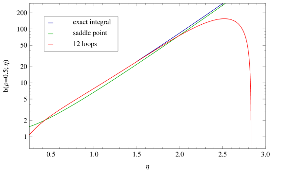
Figure 1: The transverse momentum distribution $b(\rho;\eta)$ in the high-energy limit as a function of the rapidity for $\rho=0.5$ evaluated perturbatively through twelve loops (red), and compared to the exact Mellin integral (blue) and its saddle-point approximation (green).

Remarkably, these formulas for $B_{k}(\rho)$ follow from essentially the same generating function (44) that we found for $F_{k}(w,w^{\ast})$:

$$B(\rho;\eta)=\mathcal{P}_{H}\left[\mathcal{X}(x_{0},x_{1};2\,\eta)\,\cal Z(x_{0};\eta)\right]\,.$$ (84)

The only two differences with respect to eq. (44) are that $2\eta$, not $\eta$, appears as the argument of $\mathcal{X}$, and the map $\mathcal{P}_{H}$ sends a word $\omega$ to the HPL $H_{\omega}(\rho^{2})$ instead of to the SVHPL $\cal L_{\omega}(-w,-w^{\ast})$. We have not proven this result to all orders, but we have checked that it reproduces the analytical results for the coefficients $B_{k}(\rho)$ through six loops shown in eq. (83). In addition, we have checked eq. (84) up to twelve loops numerically, by performing the integral in the Mellin representation of $b(\rho,\eta)$,

$$b(\rho;\eta)=\int_{-\infty}^{+\infty}d\nu\,\rho^{2i\nu}\,e^{\eta\,\chi_{\nu,0}}\simeq\sqrt{\frac{\pi}{14\,\zeta_{3}\,\eta}}\exp\left[4\eta\,\ln 2-\frac{\ln^{2}\rho^{2}}{56\,\zeta_{3}\,\eta}\right]\,,$$ (85)

obtained from eqs. (6) and (10) by integrating the azimuthal angle over the range $[0,2\pi]$. More precisely, we have computed the Mellin integral order-by-order in $\eta$ by closing the integration contour in the upper half plane and numerically summing up the residues. Finally, we compare the transverse momentum distribution $b(\rho;\eta)$ truncated at twelve loops, as obtained from the generating functional (84), with the exact Mellin integral and its saddle-point approximation given in eq. (85). We perform the comparison as a function of $\eta$ (i.e. the rapidity) for two selected values of $\rho$ in Fig. 1 and 2. We observe that there is a very good agreement between the exact integral and its perturbative expansion over a wide range of rapidities.

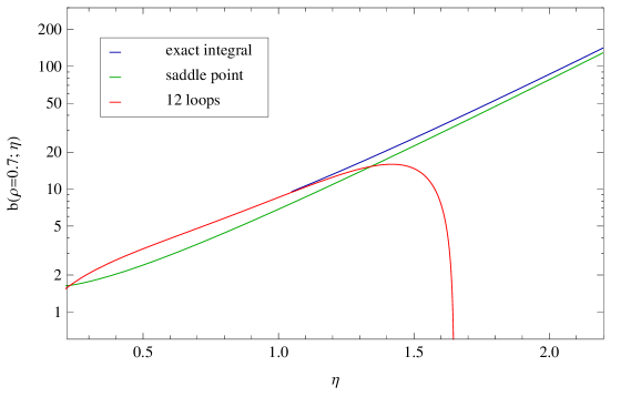
Figure 2: Same as Fig. 1, but for $\rho=0.7$.

5.3 The total cross section

We can now perform a final integration over the transverse momentum variable $\rho$. The coefficients in the perturbative expansion contain a logarithmic divergence as $\rho\rightarrow 1$, so we will cut off the integral at $\rho^{2}=1-\delta$, after mapping the integral to the region $p_{1\bot}^{2}<p_{2\bot}^{2}$, or $0<\rho<1$. We define the regulated total cross section,

$$\begin{split}\hat{\sigma}_{gg}(\delta)&\,\equiv 2\int_{E_{\bot}^{2}}^{\infty}dp_{1\bot}^{2}\int_{p_{1\bot}^{2}/(1-\delta)}^{\infty}dp_{2\bot}^{2}\frac{d\hat{\sigma}_{gg}}{dp_{1\bot}^{2}dp_{2\bot}^{2}}\\ &\,=2\int_{E_{\bot}^{2}}^{\infty}dp_{1\bot}^{2}\,p_{1\bot}^{2}\int_{0}^{1-\delta}\frac{d\rho^{2}}{\rho^{4}}\frac{d\hat{\sigma}_{gg}}{dp_{1\bot}^{2}dp_{2\bot}^{2}}\,.\end{split}$$ (86)

Using eq. (74), we have

$$\begin{split}\hat{\sigma}_{gg}(\delta)&\,=(C_{A}\alpha_{\scriptscriptstyle S})^{2}\int_{E_{\bot}^{2}}^{\infty}\frac{dp_{1\bot}^{2}}{(p_{1\bot}^{2})^{2}}\int_{0}^{1-\delta}d\rho^{2}\,\frac{b(\rho)}{2\rho}\\ &\,=\frac{\pi(C_{A}\alpha_{\scriptscriptstyle S})^{2}}{E_{\bot}^{2}}\sum_{k=1}^{\infty}\eta^{k}\int_{0}^{1-\delta}d\rho^{2}\frac{B_{k}(\rho)}{1-\rho^{2}}\,.\end{split}$$ (87)

Comparing with eq. (15), we see that

$$I_{k}(\delta)\equiv 2\int_{0}^{1-\delta}d\rho^{2}\,\frac{B_{k}(\rho)}{1-\rho^{2}}$$ (88)

should correspond to the coefficients $f_{0,k}$ in the Mueller-Navelet dijet cross section (15). However, at fixed order $k$ there will be a logarithmic divergence as $\delta\rightarrow 0$, for the reason discussed at the end of Section 5.1. As we did there, we will have to perform the sum over $k$ for the divergent terms, which will regulate the divergence. Then we can take the limit $\delta\rightarrow 0$. Whereas the discussion in Section 5.1 concerned only the leading logarithms at a given order in the $\eta$ expansion, here we will provide a (conjectured) expression accurate to all logarithmic orders.

Because the $B_{k}(\rho)$ are linear combinations of harmonic polylogarithms with argument $\rho^{2}$, the integral can be performed for any value of $\delta$, according to eq. (19), by prepending a “1” to each HPL weight vector and setting the argument to $1-\delta$. We then expand the result for small $\delta$, neglecting power-suppressed terms in $\delta$. We find the following result through nine loops,

$$I_{k}(\delta)=f_{0,k}-\sum_{m=0}^{k}Z_{m}\frac{(2\ln\delta)^{k-m}}{(k-m)!}+{\cal O}(\delta),$$ (89)

where $f_{0,k}$ are the Mueller-Navelet coefficients (16) and the $Z_{m}$ coefficients are given through seven loops by,

$$\begin{split}Z_{0}&\,=1\,,\\ Z_{1}&\,=0\,,\\ Z_{2}&\,=\zeta_{2}\,,\\ Z_{3}&\,=\frac{8}{3}\zeta_{3}\,,\\ Z_{4}&\,=\frac{19}{4}\zeta_{4}\,,\\ Z_{5}&\,=\frac{32}{5}\zeta_{5}+\frac{8}{3}\zeta_{2}\,\zeta_{3}\,,\\ Z_{6}&\,=\frac{275}{16}\zeta_{6}+\frac{32}{9}\zeta_{3}^{2}\,,\\ Z_{7}&\,=\frac{128}{7}\zeta_{7}+\frac{38}{3}\zeta_{3}\,\zeta_{4}+\frac{32}{5}\zeta_{2}\,\zeta_{5}\,.\end{split}$$ (90)

These coefficients are consistent with the following all-orders expression:

$$Z(\eta)\equiv\sum_{m=0}^{\infty}Z_{m}\eta^{m}=\exp\biggl{[}\,\sum_{k=2}^{\infty}\eta^{k}\,\Bigl{(}2^{k}-1-(-1)^{k}\Bigr{)}\,\frac{\zeta_{k}}{k}\biggr{]}=e^{-2\gamma_{E}\eta}\,\frac{\Gamma(1-2\eta)}{\Gamma(1-\eta)\,\Gamma(1+\eta)}\,,$$ (91)

where $\gamma_{E}=-\Gamma^{\prime}(1)$ denotes the Euler-Mascheroni constant. We explicitly checked that the all orders expression reproduces the correct coefficients $Z_{m}$ through 13 loops.

While each perturbative coefficient is logarithmically divergent, when we resum the series the divergence goes away:

$$\begin{split}I(\delta)\equiv\sum_{k=0}^{\infty}I_{k}(\delta)\eta^{k}&\,=\sum_{k=0}^{\infty}f_{0,k}\eta^{k}-\sum_{m=0}^{\infty}Z_{m}\eta^{m}\sum_{l=0}^{\infty}\frac{(2\eta\ln\delta)^{l}}{l!}+{\cal O}(\delta)\\ &\,=\sum_{k=0}^{\infty}f_{0,k}\eta^{k}-Z(\eta)\delta^{2\eta}+{\cal O}(\delta)\,.\end{split}$$ (92)

We now take the limit $\delta\rightarrow 0$ in the last form of this equation. This limit allows us to identify the coefficients $f_{0,k}$ in eq. (89) with the Mueller-Navelet coefficients defined in eq. (15).

Finally, the next few Mueller-Navelet coefficients can be determined analytically in this way,

$$\begin{split}f_{0,6}&\,=\frac{13}{4}\,\zeta_{3}^{2}+\frac{3737}{120}\,\zeta_{6}\,,\\ f_{0,7}&\,=-\frac{87}{5}\,\zeta_{3}\,\zeta_{4}-\frac{116}{9}\,\zeta_{2}\,\zeta_{5}-\frac{3983}{144}\,\zeta_{7}\,,\\ f_{0,8}&\,=-\frac{37}{75}\,\zeta_{5,3}+\frac{64}{15}\,\zeta_{2}\,\zeta_{3}^{2}+\frac{369}{20}\,\zeta_{5}\,\zeta_{3}+\frac{50606057}{453600}\,\zeta_{8}\,,\\ f_{0,9}&\,=-\frac{139}{60}\,\zeta_{3}^{3}-\frac{15517}{252}\,\zeta_{6}\,\zeta_{3}-\frac{3533}{63}\,\zeta_{4}\,\zeta_{5}-\frac{557}{15}\,\zeta_{2}\,\zeta_{7}-\frac{5215361}{60480}\,\zeta_{9}\,,\\ f_{0,10}&\,=-\frac{2488}{4725}\,\zeta_{5,3}\,\zeta_{2}-\frac{94721}{211680}\,\zeta_{7,3}+\frac{1948}{105}\,\zeta_{4}\,\zeta_{3}^{2}+\frac{2608}{105}\,\zeta_{2}\,\zeta_{5}\,\zeta_{3}+\frac{12099}{224}\,\zeta_{7}\,\zeta_{3}\\ &\,+\frac{1335931}{47040}\,\zeta_{5}^{2}+\frac{25669936301}{63504000}\,\zeta_{10}\,,\\ f_{0,11}&\,=\frac{62}{315}\,\zeta_{5,3}\,\zeta_{3}+\frac{83}{120}\,\zeta_{5,3,3}-\frac{2872}{945}\,\zeta_{2}\zeta_{3}^{3}-\frac{13211}{672}\,\zeta_{5}\,\zeta_{3}^{2}-\frac{661411}{3024}\,\zeta_{8}\,\zeta_{3}\\ &\,-\frac{242776937}{725760}\zeta_{11}-\frac{605321}{3024}\,\zeta_{5}\,\zeta_{6}-\frac{2583643}{16200}\,\zeta_{4}\,\zeta_{7}-\frac{28702763}{340200}\,\zeta_{2}\,\zeta_{9}\,,\\ f_{0,12}&\,=\frac{74711}{162000}\zeta_{5,3}\,\zeta_{4}-\frac{13793}{7560}\,\zeta_{6,4,1,1}+\frac{3965011}{793800}\,\zeta_{7,3}\,\zeta_{2}-\frac{33356851}{4082400}\,\zeta_{9,3}\\ &\,+\frac{252163}{181440}\,\zeta_{3}^{4}+\frac{620477}{10080}\,\zeta_{6}\,\zeta_{3}^{2}+\frac{8101339}{75600}\,\zeta_{4}\,\zeta_{5}\,\zeta_{3}+\frac{342869}{3780}\,\zeta_{2}\,\zeta_{7}\,\zeta_{3}\\ &\,+\frac{101571047}{680400}\,\zeta_{9}\,\zeta_{3}+\frac{71425871}{1587600}\,\zeta_{2}\,\zeta_{5}^{2}+\frac{904497401571619}{620606448000}\,\zeta_{12}\\ &\,+\frac{484414571}{2721600}\,\zeta_{5}\,\zeta_{7}\,,\\ f_{0,13}&\,=\frac{4513}{1890}\,\zeta_{5,3}\,\zeta_{5}+\frac{27248}{23625}\,\zeta_{5,3,3}\,\zeta_{2}-\frac{97003}{235200}\,\zeta_{5,5,3}+\frac{13411}{75600}\,\zeta_{7,3}\,\zeta_{3}\\ &\,+\frac{7997743}{12700800}\,\zeta_{7,3,3}-\frac{187318}{14175}\,\zeta_{4}\,\zeta_{3}^{3}-\frac{125056}{4725}\,\zeta_{2}\,\zeta_{5}\,\zeta_{3}^{2}-\frac{17411413}{302400}\,\zeta_{7}\,\zeta_{3}^{2}\\ &\,-\frac{5724191}{100800}\,\zeta_{5}^{2}\,\zeta_{3}-\frac{1874972477}{2376000}\,\zeta_{10}\,\zeta_{3}-\frac{2418071698069}{2235340800}\,\zeta_{13}\\ &\,-\frac{2379684877}{6048000}\,\zeta_{11}\,\zeta_{2}-\frac{297666465053}{523908000}\,\zeta_{6}\,\zeta_{7}-\frac{1770762319}{2494800}\,\zeta_{5}\,\zeta_{8}\\ &\,-\frac{229717224973}{628689600}\,\zeta_{4}\,\zeta_{9}\,.\end{split}$$ (93)

The results have been reduced to a minimal set of multiple zeta values using the multiple zeta value data mine [36]. We have checked the values (93) through 19 digits by numerically evaluating eq. (12) for $n=0$.

The Mueller-Navelet coefficients can again be obtained from a generating function similar to the one for the transverse momentum distribution,

$$\hat{\sigma}_{gg}=\frac{\pi\,(C_{A}\alpha_{\scriptscriptstyle S})^{2}}{2E_{\bot}^{2}}\,\Big{\{}Z(\eta)+2\,\cal P_{\zeta}\left[x_{1}\,\mathcal{X}(x_{0},x_{1};2\,\eta)\,\cal Z(x_{0};\eta)\right]\Big{\}}\,,$$ (94)

where $\cal P_{\zeta}$ is the linear map that sends a word to the corresponding multiple zeta value regularized by the shuffle multiplication [30] (cf. the definition of the Drinfel’d associator in Section 3). We checked that the generating function reproduces the results of eq. (93). The structure of the generating function can be understood as follows: The integral (88) adds a “1” to every HPL in $B(\rho;\eta)$, which in terms of the non-commutative variables $\{x_{0},x_{1}\}$ corresponds to multiplying by $x_{1}$ from the left. The regularized version of the integral (88) is obtained by dropping all logarithmically divergent terms, i.e., by replacing all zeta values by their shuffle-regularized version. Finally, we need to partition the regularized version of the integral into its contribution from the Mueller-Navelet coefficients and the contribution from eq. (91). The need to perform this partitioning can be seen by examining the first line of eq. (92), in which the terms at order $k$ with no powers of $\ln\delta$ are $f_{0,k}-Z_{k}$. These are the terms generated by the shuffle regularization. Therefore we have to add the $Z(\eta)$ term in order to obtain eq. (94), the generating function for the Mueller-Navelet coefficients $f_{0,k}$.

Mueller and Navelet [8] also gave an asymptotic formula for the behavior of $f_{0,k}$ as $k\rightarrow\infty$:

$$\sum_{k=0}^{\infty}\tilde{f}_{0,k}\eta^{k}=\frac{1}{\pi\nu_{0}}\biggl{[}\frac{1}{1+2\eta}-\frac{1}{8\nu_{0}^{2}(1+\frac{2}{3}\eta)}\biggr{]}\,,$$ (95)

where $\nu_{0}=e^{-\gamma_{E}}$ and $\gamma_{E}$ is the Euler-Mascheroni constant. In Table 1, we compare the numerical values of the exact coefficients $f_{0,k}$ from eq. (93) with the approximate values $\tilde{f}_{0,k}$ from this formula. We see that by $k=13$ the exact and approximate values agree to 2 parts in a billion.

$k$	$f_{0,k}$	$\tilde{f}_{0,k}$
8	145.13975384008912	145.12606589694502
9	-290.25988683555143	-290.26382715239066
10	580.53650927568371	580.53545121044840
11	-1161.07585293954502	-1161.07610035800818
12	2322.15572373880091	2322.15566600742394
13	-4644.31363149936796	-4644.31364220911962

Table 1: Numerical values of the exact coefficients $f_{0,k}$ from eq. (93), compared with the approximate values $\tilde{f}_{0,k}$ for asymptotically large $k$ from eq. (95).

6 Conclusions

In this paper, we have introduced the generating function (42) which allows us to obtain, at each order in perturbation theory, the coefficients of the leading logarithmic BFKL Green’s function in transverse momentum space. In eq. (50) we have explicitly shown the coefficients of the first six loops of that $\alpha_{\scriptscriptstyle S}$ expansion. This allows us to exhibit analytically the dependence on the jet transverse momenta of the dijet cross section in the large rapidity limit, i.e. the Mueller-Navelet jet cross section. Accordingly, we have provided fully analytic azimuthal-angle and transverse-momentum distributions of the Mueller-Navelet jet cross section in terms of harmonic polylogarithms. We have also obtained the Mueller-Navelet total cross section through a generating function, and have computed its coefficients explicitly up to 13 loops.

It would be interesting to know whether the analysis presented above can be extended to the BFKL Green’s function at next-to-leading logarithmic accuracy, either in QCD or in $\mathcal{N}=4$ super-Yang-Mills theory, for which we know that new classes of single-valued harmonic polylogarithms will appear. That is left to future work.

Appendix A A recursive formula for the Fourier coefficients $\chi_{\nu,n}$

Using the recursive formula for the $\psi$ function

$$\psi(1+z)=\psi(z)+{1\over z}\,,$$ (96)

we obtain a recursive equation for $\chi_{\nu,n}$,

$$\chi_{\nu,n+2}=\chi_{\nu,n}-{(1+n)\over\nu^{2}+\frac{(1+n)^{2}}{4}}\,,\qquad n\geq 0\,.$$ (97)

By iterating it, we can make the $\chi$ function explicit for the even and odd modes,

$$\chi_{\nu,2n} = \chi_{\nu,0}-\sum_{j=0}^{n-1}{1+2j\over\nu^{2}+\frac{(1+2j)^{2}}{4}}\,,$$

$$\chi_{\nu,2n+1} = \chi_{\nu,1}-\sum_{j=0}^{n-1}{2(j+1)\over\nu^{2}+(j+1)^{2}}\,,$$ (98)

for $n\geq 1$. Note that we have in addition $\chi_{\nu,-n}=\chi_{\nu,n}$. Then one can substitute eq. (98) into eq. (12) and obtain a recursive formula for the Fourier coefficients.

Appendix B The small $\nu$ expansion of the BFKL eigenvalue $\chi_{\nu,n}$

For small $\nu$, we can use the expansion

$$\psi(1+z)-\psi(1)\,=\,\sum_{k=2}^{\infty}(-1)^{k}\,\zeta_{k}\,z^{k-1}\,,$$ (99)

valid for small $z$, and the doubling formula,

$$2\psi(2z)=2\ln{2}+\psi(z)+\psi\left(z+\frac{1}{2}\right)\,,$$

to obtain

$$\chi_{\nu,n}\,=\,2\,\sum_{k=0}^{\infty}a_{kn}\nu^{2k}\,,$$ (100)

with coefficients

$$\begin{array}[]{ll}a_{00}=2\ln{2}\,,&\quad a_{k0}=(-1)^{k}\,(2^{2k+1}-1)\,\zeta_{2k+1}\,,\\ a_{01}=0\,,&\quad a_{k1}=(-1)^{k}\,\zeta_{2k+1}\,.\end{array}\quad\mbox{for}\quad k\neq 0\,.$$ (101)

For $n=0$, that yields the usual expansion of the eigenvalue of the BFKL equation,

$$\chi_{\nu,0}\,=\,2\,(2\ln{2}-7\zeta_{3}\nu^{2}+\cdots)\,.$$ (102)

Eq. (97) allows us to obtain a recursive formula for the coefficients of eq. (100),

$$a_{k,n+2}=a_{kn}+(-1)^{k+1}\left({2\over 1+|n|}\right)^{2k+1}\,.$$ (103)

For $k=0,1$, eq. (103) yields

$$a_{0,n+2}=a_{0n}-{2\over 1+|n|}\qquad\quad a_{1,n+2}=a_{1n}+\left({2\over 1+|n|}\right)^{3}\,,$$ (104)

in agreement with ref. [10].

We can solve the formulæ of eq. (104) explicitly, and write

$$\begin{array}[]{ll}\displaystyle a_{0,2n}=a_{00}-\sum_{k=1}^{n}{2\over 2k-1}=\psi(1)-\psi\left(n+\frac{1}{2}\right)\\ \displaystyle a_{1,2n}=a_{10}+\sum_{k=1}^{n}\left({2\over 2k-1}\right)^{3}=\frac{1}{2}\ \psi^{\prime\prime}\left(n+\frac{1}{2}\right)\\ \displaystyle a_{0,2n+1}=a_{01}-\sum_{k=1}^{n}{1\over k}=\psi(1)-\psi\left(n+1\right)\\ \displaystyle a_{1,2n+1}=a_{11}+\sum_{k=1}^{n}\left({1\over k}\right)^{3}=\frac{1}{2}\ \psi^{\prime\prime}\left(n+1\right)\end{array}\qquad\mbox{with}\quad n\geq 1\,,$$ (105)

and with $a_{00},a_{01},a_{10},a_{11}$ given in eq. (101).

References

- [1] E. A. Kuraev, L. N. Lipatov, and V. S. Fadin, Multi-Reggeon processes in the Yang-Mills theory, Sov. Phys. JETP 44 (1976) 443.
- [2] E. A. Kuraev, L. N. Lipatov, and V. S. Fadin, The Pomeranchuk singularity in nonabelian gauge theories, Sov. Phys. JETP 45 (1977) 199.
- [3] I. I. Balitsky and L. N. Lipatov, The Pomeranchuk singularity in quantum chromodynamics, Sov. J. Nucl. Phys. 28 (1978) 822.
- [4] L. N. Lipatov, Reggeization of the vector meson and the vacuum singularity in nonabelian gauge theories, Sov. J. Nucl. Phys. 23 (1976) 338.
- [5] V. S. Fadin and L. N. Lipatov, BFKL pomeron in the next-to-leading approximation, Phys. Lett. B429 (1998) 127, [hep-ph/9802290].
- [6] G. Camici and M. Ciafaloni, Irreducible part of the next-to-leading BFKL kernel, Phys. Lett. B412 (1997) 396, [hep-ph/9707390].
- [7] M. Ciafaloni and G. Camici, Energy scale(s) and next-to-leading BFKL equation, Phys. Lett. B430 (1998) 349, [hep-ph/9803389].
- [8] A. H. Mueller and H. Navelet, An inclusive minijet cross-section and the bare pomeron in QCD, Nucl.Phys. B282 (1987) 727.
- [9] V. Del Duca and C. R. Schmidt, Dijet production at large rapidity intervals, Phys.Rev. D49 (1994) 4510, [hep-ph/9311290].
- [10] W. J. Stirling, Production of jet pairs at large relative rapidity in hadron hadron collisions as a probe of the perturbative pomeron, Nucl.Phys. B423 (1994) 56, [hep-ph/9401266].
- [11] V. Del Duca and C. R. Schmidt, BFKL versus corrections to large rapidity dijet production, Phys.Rev. D51 (1995) 2150, [hep-ph/9407359].
- [12] V. Del Duca and C. R. Schmidt, Azimuthal angle decorrelation in large rapidity dijet production at the Tevatron, Nucl.Phys.Proc.Suppl. 39BC (1995) 137, [hep-ph/9408239].
- [13] L. H. Orr and W. J. Stirling, Dijet production at hadron hadron colliders in the BFKL approach, Phys.Rev. D56 (1997) 5875, [hep-ph/9706529].
- [14] C. R. Schmidt, A Monte Carlo solution to the BFKL equation, Phys.Rev.Lett. 78 (1997) 4531, [hep-ph/9612454].
- [15] J. Andersen, V. Del Duca, S. Frixione, C. Schmidt, and W. J. Stirling, Mueller-Navelet jets at hadron colliders, JHEP 0102 (2001) 007, [hep-ph/0101180].
- [16] J. R. Andersen, On the role of NLL corrections and energy conservation in the high energy evolution of QCD, Phys.Lett. B639 (2006) 290, [hep-ph/0602182].
- [17] D. Colferai, F. Schwennsen, L. Szymanowski, and S. Wallon, Mueller Navelet jets at LHC - complete NLL BFKL calculation, JHEP 1012 (2010) 026, [1002.1365].
- [18] B. Ducloue, L. Szymanowski, and S. Wallon, Confronting Mueller-Navelet jets in NLL BFKL with LHC experiments at 7 TeV, JHEP 1305 (2013) 096, [1302.7012].
- [19] D0 Collaboration, B. Abbott et al., Probing BFKL dynamics in the dijet cross section at large rapidity intervals in collisions at GeV and 630-GeV, Phys.Rev.Lett. 84 (2000) 5722, [hep-ex/9912032].
- [20] ATLAS Collaboration, G. Aad et al., Measurement of dijet production with a veto on additional central jet activity in collisions at TeV using the ATLAS detector, JHEP 1109 (2011) 053, [1107.1641].
- [21] CMS Collaboration, S. Chatrchyan et al., Ratios of dijet production cross sections as a function of the absolute difference in rapidity between jets in proton-proton collisions at TeV, Eur.Phys.J. C72 (2012) 2216, [1204.0696].
- [22] D0 Collaboration, S. Abachi et al., The azimuthal decorrelation of jets widely separated in rapidity, Phys.Rev.Lett. 77 (1996) 595, [hep-ex/9603010].
- [23] CMS Collaboration, S. Chatrchyan et al., Azimuthal angle decorrelations of jets widely separated in rapidity in pp collisions at TeV, CMS PAS FSQ-12-002.
- [24] L. J. Dixon, C. Duhr, and J. Pennington, Single-valued harmonic polylogarithms and the multi-Regge limit, JHEP 1210 (2012) 074, [1207.0186].
- [25] J. Pennington, The six-point remainder function to all loop orders in the multi-Regge limit, JHEP 1301 (2013) 059, [1209.5357].
- [26] F. C. S. Brown, Single-valued multiple polylogarithms in one variable, C. R. Acad. Sci. Paris, Ser. I 338 (2004) 527.
- [27] F. Brown, Single-valued periods and multiple zeta values, 1309.5309.
- [28] E. Remiddi and J. Vermaseren, Harmonic polylogarithms, Int.J.Mod.Phys. A15 (2000) 725, [hep-ph/9905237].
- [29] V. Knizhnik and A. Zamolodchikov, Current algebra and Wess-Zumino model in two-dimensions, Nucl.Phys. B247 (1984) 83.
- [30] K. Ihara, M. Kaneko, and D. Zagier, Derivation and double shuffle relations for multiple zeta values, Compositio Math. 142 (2006) 307.
- [31] K. T. Chen, Iterated path integrals, Bull. Amer. Math. Soc. 83 (1977) 831.
- [32] F. C. S. Brown, Multiple zeta values and periods of moduli spaces , Annales scientifiques de l’ENS 42 (2009), no. 3 371, [math/0606419].
- [33] A. B. Goncharov, A simple construction of Grassmannian polylogarithms, 0908.2238.
- [34] A. B. Goncharov, M. Spradlin, C. Vergu, and A. Volovich, Classical polylogarithms for amplitudes and Wilson loops, Phys.Rev.Lett. 105 (2010) 151605, [1006.5703].
- [35] C. Duhr, H. Gangl, and J. R. Rhodes, From polygons and symbols to polylogarithmic functions, JHEP 1210 (2012) 075, [1110.0458].
- [36] J. Blümlein, D. Broadhurst, and J. Vermaseren, The Multiple Zeta Value Data Mine, Comput.Phys.Commun. 181 (2010) 582–625, [0907.2557].