Gravitational collapse of a homogeneous scalar field in deformed phase space

Abstract

We study the gravitational collapse of a homogeneous scalar field, minimally coupled to gravity, in the presence of a particular type of dynamical deformation between the canonical momenta of the scale factor and of the scalar field. In the absence of such a deformation, a class of solutions can be found in the literature [R. Goswami and P. S. Joshi, arXiv:gr-qc/0410144], whereby a curvature singularity occurs at the collapse end state, which can be either hidden behind a horizon or be visible to external observers. However, when the phase-space is deformed, as implemented herein this paper, we find that the singularity may be either removed or instead, attained faster. More precisely, for negative values of the deformation parameter, we identify the emergence of a negative pressure term, which slows down the collapse so that the singularity is replaced with a bounce. In this respect, the formation of a dynamical horizon can be avoided depending on the suitable choice of the boundary surface of the star. Whereas for positive values, the pressure that originates from the deformation effects assists the collapse toward the singularity formation. In this case, since the collapse speed is unbounded, the condition on the horizon formation is always satisfied and furthermore the dynamical horizon develops earlier than when the phase-space deformations are absent. These results are obtained by means of a thoroughly numerical discussion.

I Introduction

One of the most important contemporary challenges in gravitation theory and relativistic astrophysics is to fully describe the gravitational collapse of a massive body from initially regular matter distributions Frolov . While Einstein’s general theory of relativity has been a highly successful theory in describing gravitation, it is a well-established result that a gravitational collapse process, governed by the Einstein field equations with physically reasonable matter configurations, may induce a spacetime singularity to appear Hawking : physical parameters such as the matter energy density and spacetime curvatures will diverge. Among the variety of models that have been investigated, the gravitational collapse of scalar fields have attracted particular attention: massless as well as massive scalar fields have been studied by applying analytical and numerical methods Wym81 -GJM12 . However, classical general relativity breaks down at the very late stages of a collapse scenario, where densities and curvatures are so extreme that quantum gravity effects may become more prominent, therefore possibly resolving the classical singularity QGS ; in .

One such possible effect is noncommutativity between spacetime coordinates, which was first proposed by Snyder SNY in an effort to introduce a short length cutoff (the noncommutativity parameter) in a Lorentz covariant way. The aim was to improve the renormalizability properties of relativistic quantum field theory (see noncom and references therein). The basic idea that lies behind noncommutativity is to take into account the uncertainty in simultaneous measurements of any (canonical) pair of phase space variables and their conjugate momenta. This idea has been revived in recent years, due to strong motivations from string and M-theories STMT and more concretely has been proposed in a new algebra regarding spacetime uncertainty relations derived from quantum mechanics and general relativity that provides the framework for noncommutative field theories in a Lorentz covariant way DFR (see also DFR1 and references therein). One may also study noncommutative theories in particle physics, owing to the interesting predictions having been made in this area, such as IR/UV mixing and nonlocality IRUV , violation of Lorentz symmetry LV (see also phrev on the phenomenological features of noncommutative geometry), new physics at very short distance scales noncom and the equivalence between translations in noncommutative gauge theories and gauge transformations TRN . Noncommutative extensions of quantum mechanical models such as the harmonic oscillator HO , Hydrogen atom spectra HAS , and gravitational radiation GW have also been investigated in order to predict theoretical values of the noncommutative parameter as a test bed for the experiments.

Since the advent of noncommutative field theory, the interest in this area slowly but continuously made progress into the domain of gravity theories. Recent progresses in noncommutative geometry imply that, the noncommutative effects in general relativity may be taken into account by keeping the standard form of the Einstein tensor on the left-hand side of the field equations and introducing a modified energy-momentum tensor as a source including noncommutative parameter, on the right-hand side BHEva . Several investigations have also been carried out to verify the possible role of noncommutativity in cosmological scenarios such as Newtonian cosmology NCNC , cosmological perturbation theory and inflationary cosmology NONCOMINF , noncommutative gravity NONGRAV , quantum cosmology NONCOMQC ; BP04 and noncommutativity based on generalized uncertainty principle GUP (see NCG for reviews on different approaches to noncommutative gravity). The concept of spacetime underlying the general theory of relativity would not be sensible below the distances which are comparable to the Planck ones, because the uncertainty principle governing the quantum theory of gravity prohibits measurements in positions to better accuracies than the Plank length. Since the transition from classical to quantum mechanics requires the physical observables to be noncommutative, it is expected that, in a transition from classical to quantum gravity, the observables could also become noncommutative. Thus, by extending general relativity toward noncommutative spacetime, we may come closer to some aspects of quantum gravity. In particular, replacing the usual canonical Poisson brackets between physical variables, by others, with new terms, as suggested by string theory, concerning fundamental interactions (see e.g. STRNON and reference therein). Such deformations on the structure of the phase-space Za05 have been employed as a means to convey noncommutativity into the dynamics R.book04 -COR02 . In this work, our objective is to investigate the gravitational collapse of a minimally coupled scalar field $\phi$ in the presence of a specific phase space deformation. In particular, this modification will concern the dynamical sector involving the momenta of the scale factor $a$ and of $\phi$. Our paper is organized as follows. In Sec.  II, we briefly summarize some features regarding the gravitational collapse of a minimally coupled homogeneous scalar field JG04 , but within a Hamiltonian formalism. In Sec. III, we will obtain, still using the Hamiltonian formalism, the equations of motion for such minimally coupled scalar field, but in the presence of the particular dynamical deformation aforementioned. Subsequently, we extract (numerically) a class of solutions that represent a gravitational collapse. In particular, we discuss the implications regarding the collapse outcome, for different ranges of the deformation parameter. We will find that the deformation determines that an extra pressure term may appear, changing the collapse dynamics and whether if a singularity can be formed or not. We summarize our conclusions in Sec. IV. Appendices A and B provide complementary information regarding the equations of motion in the deformed phase-space.

II Gravitational Collapse of a Homogeneous Scalar Field

In this section, we briefly describe the gravitational collapse of a homogeneous scalar field, minimally coupled to gravity. The full detailed analysis is present in JG04 . In this work we employ the Hamiltonian formalism, for the reason that it will prove useful when we introduce, in the next section, the deformation (noncommutativity) in the phase-space. Therefore, we start with a Lagrangian density as

$${\mathcal{L}}=\sqrt{-g}\left(\frac{{\cal{R}}}{2k^{2}}-\frac{1}{2}g^{\mu\nu}\phi_{,\mu}\phi_{,\nu}-V(\phi)\right),$$ (1)

where $k^{2}\equiv 8\pi G$, ${\cal{R}}$ is the Ricci scalar, $g$ is the determinant of a metric $g_{\mu\nu}$ (where the Greek indices run from zero to three) and $V(\phi)$ is a scalar potential. For practical reasons we employ, for our gravitational setting, a spherically symmetric homogeneous collapsing (interior) region, which is given by the following line element as (cf. JG04 , JGS-LQ -PL )

$$ds^{2}=h_{ab}dx^{a}dx^{b}+R^{2}(t,r)d\Omega^{2},$$ (2)

where $h_{ab}={\rm diag}[-N^{2}(t),a^{2}(t)]$ is the line element on the two-dimensional hypersurface, normal to the two dimensional sphere characterized by the standard line element $d\Omega^{2}$. $N(t)$ is a lapse function, $a(t)$ is the scale factor, and $R(t,r)=ra(t)$ is the physical radius of the collapsing star. Hence, the scalar field must depend only on the comoving time, i.e $\phi=\phi(t)$. By substituting the Ricci scalar associated to the metric (2) into the Lagrangian density (1), neglecting the total time derivative $k^{2}d(N^{-1}a^{2}\dot{a})/dt$, the corresponding Hamiltonian reads

$${\mathcal{H}}_{0}=-\frac{k^{2}}{12}Na^{-1}P_{a}^{2}+\frac{1}{2}Na^{-3}P_{\phi}^{2}+Na^{3}V(\phi),$$ (3)

where $P_{a}$ and $P_{\phi}$ are the momentum conjugates associated to the scale factor and scalar field, respectively. Therefore, the Dirac Hamiltonian is given by

$${\mathcal{H}}={\mathcal{H}}_{0}+\lambda P_{N},$$ (4)

where we should note that, as the momentum conjugate to $N(t)$, $P_{N}$, vanishes, we have therefore added the last term, $\lambda P_{N}$ as a constraint to the Hamiltonian (3), in which $\lambda$ is a Lagrange multiplier.

Let us consider the ordinary phase-space structure described by the usual (nonvanishing) Poisson brackets, as

$$\{a,P_{a}\}=\{\phi,P_{\phi}\}=\{N,P_{N}\}=1.$$ (5)

The equations of motion with respect to the Hamiltonian (4) are

$$\dot{a}\!\!\! = \!\!\!\{a,{\mathcal{H}}\}=-\frac{k^{2}}{6}Na^{-1}P_{a},$$ (6)

$$\dot{P}_{a}\!\!\! = \!\!\!\{P_{a},{\mathcal{H}}\}=-\frac{k^{2}}{12}Na^{-2}P_{a}^{2}+\frac{3}{2}Na^{-4}P_{\phi}^{2}$$ (7)

$$- 3Na^{2}V(\phi),$$

$$\dot{\phi}\!\!\! = \!\!\!\{\phi,{\mathcal{H}}\}=Na^{-3}P_{\phi},$$ (8)

$$\dot{P}_{\phi}\!\!\! = \!\!\!\{P_{\phi},{\mathcal{H}}\}=-Na^{3}\frac{dV_{\phi}}{d\phi},$$ (9)

$$\dot{N}\!\!\! = \!\!\!\{N,{\mathcal{H}}\}=\lambda,$$ (10)

$$\dot{P}_{N}\!\!\! = \!\!\!\{P_{N},{\mathcal{H}}\}=\frac{k^{2}}{12}a^{-1}P_{a}^{2}-\frac{1}{2}a^{-3}P_{\phi}^{2}$$ (11)

$$- a^{3}V(\phi).$$

We will work in the comoving gauge, that is, we fix $N=1$. Also, to satisfy the constraint $P_{N}=0$ at all times, the secondary constraint $\dot{P}_{N}=0$ should also be satisfied. Hence, it is straightforward to show that Eqs. (6)-(11) give the dynamic evolution for the system, as

$$H^{2}=\frac{k^{2}}{3}\left[\frac{1}{2}\dot{\phi}^{2}+V(\phi)\right]\equiv\frac{k^{2}}{3}\rho(t),$$ (12)

$$2\frac{\ddot{a}}{a}+H^{2}=-k^{2}\left[\frac{1}{2}\dot{\phi}^{2}-V(\phi)\right]\equiv-k^{2}p(t),$$ (13)

while the scalar field satisfies the Klein-Gordon equation

$$\ddot{\phi}+3H\dot{\phi}+\frac{dV}{d\phi}=0,$$ (14)

where $H=\dot{a}/a=\dot{R}/R$ is the rate of collapse. In addition, $\rho$ and $p$ represent the energy density and pressure, respectively. For $\dot{\phi}\neq 0$, we can easily derive the Klein-Gordon equation (14) from the Eqs. (12) and (13) or, equivalently, from the conservation equation; thus, only two of the three Eqs. (12)-(14) are independent.

Let us rewrite Eqs. (12)-(14) in a more convenient form, as

$$H^{2} \!\!\!\!=\frac{k^{2}}{3}\left[\frac{1}{2}a^{2}H^{2}\phi_{,a}^{2}+V(\phi)\right],$$ (15)

$$3H^{2} \!\!\!+2aHH_{,a}\!=\!-k^{2}\left[\frac{1}{2}a^{2}H^{2}\phi_{,a}^{2}-V(\phi)\right],$$ (16)

$$\frac{dV}{da}\!\!\!\!\!\! = \!\!\!\!\!\!-4aH^{2}\phi_{,a}^{2}-a^{2}HH_{,a}\phi_{,a}^{2}-a^{2}H^{2}\phi_{,a}\phi_{,aa},$$

where “$,a$” $\equiv\ d/da$. The above set of differential equations have a general solution

$$H(a)\!\! = \!\!\alpha\exp\left[-\frac{k^{2}}{2}\int a\phi_{,a}^{2}da\right],$$ (18)

$$V(a)\!\! = \!\!\alpha^{2}\left(\frac{3}{k^{2}}-\frac{a^{2}}{2}\phi_{,a}^{2}\right)$$

$$\times \exp\left[-k^{2}\int a\phi_{,a}^{2}da\right],$$

where $\alpha$ is an integration constant. In order to proceed, we need to further specify the dependence of the scalar field upon one of the other variables. Thus we take the following ansatz for the scalar field, which will induce a suitable gravitational collapse dynamics:

$$\phi(a)=\sqrt{-2\beta}\ln(a),$$ (20)

where $\beta<0$ is another constant. Applying (20), we can then easily solve for the rate of collapse and the scalar field potential, to get (we set $k^{2}=1$)

$$H(a) = \alpha a^{\beta},$$ (21)

$$V(\phi) = \alpha^{2}\left(3+\beta\right){\rm exp}\left(-\sqrt{-2\beta}\phi\right),$$ (22)

where we require, additionally, that $\alpha<0$. From (21), the scale factor reads

$$a(t)=\left[a_{i}^{-\beta}-\alpha\beta(t-t_{i})\right]^{-\frac{1}{\beta}},\hskip 11.38109ptt_{s}=t_{i}+\frac{a_{i}^{-\beta}}{{\alpha\beta}},$$ (23)

where $t_{s}$ stands for the time at which the collapse ends in a spacetime singularity. Let us be more concrete. The scalar field is given by

$$\phi(t)\!=\!\mp\sqrt{\frac{-2}{\beta}}\ln\left[a_{i}^{-\beta}-\alpha\beta(t-t_{i})\right].$$ (24)

We then have the following expressions for the energy density and Kretschmann invariant as

$$\rho\!\!\! = \!\!\!3\alpha^{2}\left[a_{i}^{-\beta}-\alpha\beta(t-t_{i})\right]^{-2},$$ (25)

$$K\!\!\! = \!\!\!12\left[\left(\frac{\ddot{a}}{a}\right)^{2}+\left(\frac{\dot{a}}{a}\right)^{4}\right]$$ (26)

$$= \frac{24\alpha^{4}\left(1+\beta\left(1+\frac{\beta}{2}\right)\right)a_{i}^{4\beta}}{\left[1-(t-t_{i})\alpha\beta a_{i}^{\beta}\right]^{4}}.$$

The above class of collapse solutions has been found in JG04 , where it was shown that a spacetime singularity occurs, which can be either hidden behind the event horizon (black hole) or visible to the outside observers (naked singularity). It is the causal structure of trapped surfaces and the apparent horizon, which is the outermost boundary of the trapped region, that determines the visibility or otherwise of the spacetime singularity. If the trapped surfaces form prior to the singularity formation, then the collapse scenario ends in a black hole and if the trapped surfaces are delayed or failed to form until the singularity formation, the regimes with extreme curvature and density may be seen by the outside observers (naked singularity). Let us be clear and to that aim we introduce the null coordinates

$$d\xi^{+} = -\frac{1}{\sqrt{2}}\left[N(t)dt-a(t)dr\right],$$

$$d\xi^{-} = -\frac{1}{\sqrt{2}}\left[N(t)dt+a(t)dr\right].$$ (27)

Metric (2) can be cast into double null form as

$$ds^{2}=-2d\xi^{+}d\xi^{-}+R(t,r)^{2}d\Omega^{2}.$$ (28)

We assume, a spacetime which is time orientable and $\partial_{\pm}=\partial/\partial\xi^{\pm}$ are future pointing. The condition for radial null geodesics, $ds^{2}=0$, shows that there exist two kinds of future pointing null geodesics corresponding to $\xi^{+}={\rm constant}$ and $\xi^{-}={\rm constant}$ such that their expansion reads

$$\Theta_{\pm}=\frac{2}{R}\partial_{\pm}R.$$ (29)

The expansion of radial null geodesics is a measure that the light signals, being normal to the two-dimensional sphere, are diverging ($\Theta_{\pm}>0$) or converging ($\Theta_{\pm}<\leavevmode\nobreak\ 0$). The spacetime is said to be trapped, untrapped or marginally trapped if, respectively TRHAT ,M-Shay

$$\Theta_{+}\Theta_{-}>0,\leavevmode\nobreak\ \leavevmode\nobreak\ \leavevmode\nobreak\ \leavevmode\nobreak\ \Theta_{+}\Theta_{-}<0,\leavevmode\nobreak\ \leavevmode\nobreak\ \leavevmode\nobreak\ \leavevmode\nobreak\ \Theta_{+}\Theta_{-}=0,$$ (30)

where the third class characterizes the outermost boundary of the trapped region, the apparent horizon. Furthermore, the Misner-Sharp energy may be defined as M-Shay

$$M(t,r) = \frac{R(t,r)}{2}\left[1-h^{ab}\partial_{a}R(t,r)\partial_{b}R(t,r)\right]$$ (31)

$$= \frac{R(t,r)}{2}\left[1+\frac{R^{2}(t,r)}{2}\Theta_{+}\Theta_{-}\right],$$

which in our model reads $2M(t,r)=R(t,r)\dot{R}^{2}(t,r)$. Therefore, the dynamical apparent horizon, which is a marginally trapped surface in a spherically symmetric spacetime, is given by

$$\frac{2M}{R}=1.$$ (32)

From (31) we then conclude that the spacetime region where $2M/R>1(<1)$ is trapped (untrapped). For the solution (21), we have

$$\frac{2M(t,r)}{R(t,r)}=r^{2}\alpha^{2}a^{2(1+\beta)}.$$ (33)

We now find that for $-1<\beta<0$, if the ratio $2M(t,r)/R(t,r)$ is less than one at the initial time, it would stay less than one until the singular epoch and thus trapped surfaces fail to form throughout the collapse process. For $\beta<-1$, trapped surfaces do form and the singularity is necessarily covered by the spacetime event horizon.

We subsequently show in the next section, by resorting to phase-space deformation effects, that the corresponding gravitational collapse procedure not only does not culminate in the formation of a spacetime singularity but also exhibits a bouncing behavior, with which trapped surfaces do not form.

III Effects of phase-space deformation on collapse dynamics and singularity avoidance

From arguments based on the Wigner quasidistribution function and the Weyl correspondence between quantum-mechanical operators in Hilbert space and ordinary $c$-number functions in phase-space (see e.g. Za05 and references therein), it has been claimed that a deformation in phase space can be applied as an alternative path to quantization. More specifically, Moyal brackets, that are based on the Moyal product BP04 ,COR02 ,LORS06 ,KJS06 , have been applied to introduce the deformation in the usual phase space structure. In practice, for introducing such deformations, specific Poisson brackets are employed, wherein noncommutative effects are induced. However, for the purpose of tracing the effects of such noncommutativity in gravity, a fundamental length is usually considered in the hope of seeking for a fundamental theory upon which general relativity and quantum theory can be consistently reconciled. The so-called Planck scale is the scale at which gravitational effects become comparable to the quantum ones DFR . Such a regime with extreme energy scale or equivalently with a tiny size scale occurs in the very early universe and in the late stages of a typical gravitational collapse of a dense star.

In this regard, much effort has been devoted to the concept of spacetime noncommutativity and one of the main streams under investigation is the $\kappa$-Minkowski spacetime 7-32-star-product so that as it is shown in QGKappa , it can appear in the framework of quantum gravity coupled to matter fields. From a phenomenological standpoint, $\kappa$-Minkowski spacetime provides a suitable playground area for testing the predictions arising from deformed (doubly) special relativity (DSR) theories Ame01 -Kowa05 . In particular, the DSR is related to the $\kappa$-deformation Kowa02 . It is believed that the noncommutativity introduced in this manner is generally compatible with Lorentz symmetry Kowa02 ; RVS07 . The $\kappa$-Minkowski space is naturally introduced by concepts based on the $\kappa$-Poincare algebra Ame02 -Kowa05 , in which the ordinary brackets between coordinates are replaced by

$$\{x_{0},x_{i}\}=\frac{1}{\kappa}x_{i}.$$ (34)

The parameter $\kappa=\epsilon/\zeta$, where $\epsilon=\pm 1$ BAK01 , conveys the presence of the deformation (noncommutativity), with dimension of mass in the units $c=\hbar=1$, such that one can interpret $\kappa$ and $\zeta$ as dimensional parameters for fundamental energy and length, respectively. Within cosmology, a few publications (see e.g. KS08 ; GSS11 ) are present in the literature, using a few such types of modifications in the phase-space structure, inspired by relation (34).

However, in this section, inspired by the mentioned motivations in Ref. RFK11 and also by the corrections from string theory to Einstein gravity sheikh , we propose to change the structure of the phase-space by introducing noncommutativity between conjugate momenta to trace the deformation implications in the gravitational collapse of a homogeneous scalar field. To retrieve a model with deformation (in the phase-space), where the calculations would allow interesting novel results, but that do not convey a mere trivial scenario, we should reasonably pick a convenient framework. Therefore, we choose to employ a dynamical deformation within the canonical conjugate momentum sector, viz., with $P_{a},P_{\phi}$ replaced by new $P^{\prime}_{a^{\prime}},P^{\prime}_{\phi^{\prime}}$ momenta, that comply instead to

$$\{P^{\prime}_{a^{\prime}},P^{\prime}_{\phi^{\prime}}\}=\ell\phi^{\prime 3},$$ (35)

where we leave the other Poisson brackets unchanged [corresponding to those presented in relation (5)], with respect to the above primed variables. It is straightforward to show that the Jacobi identity is still satisfied. In RFK11 , a discussion on the motivations for choosing such kind of deformation in the phase space was presented. We shall keep the Hamiltonian with the same functional form as (3), but now written in terms of primed (deformed) variables as

$${\mathcal{H}^{\prime}}_{0}=-\frac{1}{12}N^{\prime}a^{\prime-1}P_{a^{\prime}}^{\prime 2}+\frac{1}{2}N^{\prime}a^{\prime-3}P_{\phi^{\prime}}^{\prime 2}+N^{\prime}a^{\prime 3}V^{\prime}(\phi^{\prime}{}),$$ (36)

where the standard Poisson brackets (for the primed variables) are satisfied except in  (35). Here, we aim to obtain the equations of motion for the primed variables, in which the Dirac Hamiltonian in the deformed phase-space reads

$${\mathcal{H}}^{{}^{\prime}}={\mathcal{H}}_{0}^{{}^{\prime}}+\lambda^{\prime}P^{\prime}_{N^{\prime}},$$ (37)

where ${\mathcal{H}}_{0}^{{}^{\prime}}$ is given by (36) and as $P^{\prime}_{N^{\prime}}=0$. We have added the last term, $\lambda^{\prime}P^{\prime}_{N^{\prime}}$, as a constraint to the Hamiltonian (36), in which $\lambda^{\prime}$ is a Lagrange multiplier and $P^{\prime}_{N^{\prime}}$ is the momentum conjugate to $N^{\prime}(t)$. By recalling that the deformed phase structure is described by the deformed (nonvanishing) Poisson brackets (35) and $\{a^{\prime},P^{\prime}_{a^{\prime}}\}=\{\phi^{\prime},P^{\prime}_{\phi^{\prime}}\}=\{N^{\prime},P^{\prime}_{N^{\prime}}\}=1$, the equations of motion with respect to Hamiltonian (37) are given by

$$\dot{a^{\prime}}\!\!\! = \!\!\!\{a^{\prime},{\mathcal{H^{\prime}}}\}=-\frac{1}{6}N^{\prime}a^{\prime-1}P^{\prime}_{a^{\prime}},$$ (38)

$$\dot{P^{\prime}}_{a^{\prime}}\!\!\! = \!\!\!\{P^{\prime}_{a^{\prime}},{\mathcal{H^{\prime}}}\}=-\frac{1}{12}N^{\prime}a^{\prime-2}P_{a^{\prime}}^{{}^{\prime}2}+\frac{3}{2}N^{\prime}a^{\prime-4}P_{\phi^{\prime}}^{{}^{\prime}2}$$ (39)

$$- 3N^{\prime}a^{{}^{\prime}2}V^{\prime}(\phi^{\prime})+N^{\prime}\ell a^{\prime-3}\phi^{\prime 3}P^{\prime}_{\phi^{\prime}},$$

$$\dot{\phi^{\prime}}\!\!\! = \!\!\!\{\phi^{\prime},{\mathcal{H^{\prime}}}\}=N^{\prime}a^{\prime-3}P^{\prime}_{\phi^{\prime}},$$ (40)

$$\dot{P^{\prime}}_{\phi^{\prime}}\!\!\! = \!\!\!\{P^{\prime}_{\phi^{\prime}},{\mathcal{H^{\prime}}}\}=-N^{\prime}a^{\prime 3}\frac{dV^{\prime}_{\phi^{\prime}}}{d\phi^{\prime}}$$ (41)

$$+ \frac{1}{6}N^{\prime}\ell a^{\prime-1}\phi^{\prime 3}P^{\prime}_{a^{\prime}},$$

$$\dot{N^{\prime}}\!\!\! = \!\!\!\{N^{\prime},{\mathcal{H^{\prime}}}\}=\lambda^{\prime},$$ (42)

$$\dot{P^{\prime}}_{N^{\prime}}\!\!\! = \!\!\!\{P^{\prime}_{N^{\prime}},{\mathcal{H^{\prime}}}\}=\frac{1}{12}a^{\prime-1}P_{a^{\prime}}^{{}^{\prime}2}-\frac{1}{2}a^{\prime-3}P_{\phi^{\prime}}^{{}^{\prime}2}$$ (43)

$$- \!\!\!a^{\prime 3}V^{\prime}(\phi^{\prime}).$$

Again, we work in the comoving gauge, i.e, we set $N^{\prime}=1$. Also, the constraint $P^{\prime}_{N^{\prime}}=0$ gives $\dot{P^{\prime}}_{N^{\prime}}=0$. Hence, from (43), we obtain

$$P_{a^{\prime}}^{{}^{\prime}2}=6a^{\prime-2}P_{\phi^{\prime}}^{{}^{\prime}2}+12a^{\prime 4}V^{\prime}(\phi^{\prime}).$$ (44)

By squaring both sides of Eq. (38) and substituting $P_{a^{\prime}}^{{}^{\prime}2}$ from (44) and then using Eq. (40), we get the Hamiltonian constraint as

$$\left(\frac{\dot{a^{\prime}}}{a^{\prime}}\right)^{2}=\frac{1}{3}\left[\frac{1}{2}\dot{\phi^{\prime}}^{2}+V^{\prime}(\phi^{\prime})\right]\equiv\frac{1}{3}\rho^{\prime}_{{\rm eff}}.$$ (45)

Now, differentiating Eq. (38) with respect to the time, and then employing Eqs. (39), (40), (44) and (45) we have

$$2\frac{\ddot{a^{\prime}}}{a^{\prime}}+\left(\frac{\dot{a^{\prime}}}{a^{\prime}}\right)^{2}\!\!\! = \!\!\!-\left[\frac{1}{2}\dot{\phi^{\prime}}^{2}-V^{\prime}(\phi^{\prime})\right]$$

$$- \!\!\!\frac{1}{3}\ell a^{\prime-2}\phi^{\prime 3}\dot{\phi^{\prime}}\equiv-(p^{\prime}+p^{\prime}_{{\rm d}})\equiv-p^{\prime}_{{\rm eff}},$$

where $p^{\prime}_{{\rm d}}\equiv 1/3\ell a^{\prime-2}\phi^{\prime 3}\dot{\phi^{\prime}}$ refers to an effective pressure term associated to effects arising from the deformation parameter. Finally, a modified Klein-Gordon equation can be derived if we differentiate both sides of (40) with respect to time. Then, if we substitute for $\dot{P^{\prime}_{\phi^{\prime}}}$ from (41) into the resulted expression and using relation (38), we extract

$$\ddot{\phi^{\prime}}+3\left(\frac{\dot{a^{\prime}}}{a^{\prime}}\right)\dot{\phi^{\prime}}+\frac{dV^{\prime}(\phi^{\prime})}{d\phi^{\prime}}+\ell\dot{a^{\prime}}\left(\frac{\phi^{\prime}}{a^{\prime}}\right)^{3}=0.$$ (47)

Note that, in all of the above equations, if we set $\ell=0$, then, each primed equation (quantity/variable) will have the same form as its corresponding standard in the previous section. In fact, Eqs. (45)–(47) (where only two of them are independent), are the extended versions of the standard equations of motion (12)–(14). These equations are associated to the deformed phase-space and their solutions will describe the behavior of the primed variables. However, hereafter, for the sake of simplicity, we drop the prime from all the variables. We should mention that, from now on, the herein unprimed quantities [which are the generalized (deformed) forms of the standard (unprimed) ones] are reduced to their corresponding in the previous section only by setting the deformation parameter equal to zero. In Appendix A, we will present another different approach for deriving the equations of motion. We should note that, although not explicit, the effects of the chosen deformation on Eq. (47) are implicit, as some of the following figures will show (in particular, cf. Figs. 1 and 6, herein).

We now investigate some aspects of the gravitational collapse, within the above framework for deformed phase-space, by means of numerical methods. We are particularly interested in probing the behavior of the scale factor, its time derivative, collapse acceleration, the scalar field evolution, and other related quantities for a potential of the same type as (22), in order to properly contrast the presence of noncommutative features in the collapse dynamics.

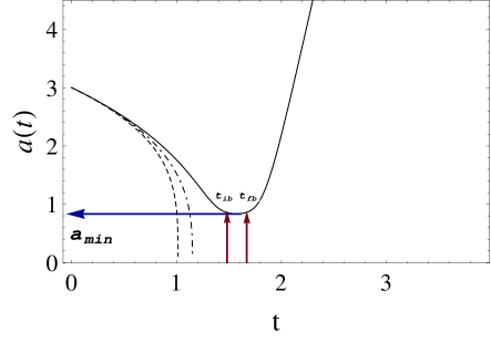
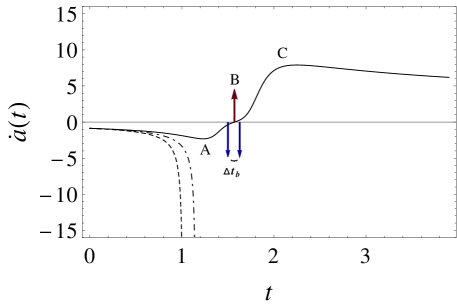
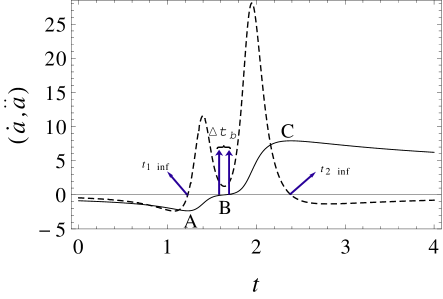
Figure 1: Upper and middle panels: The time behavior of the scale factor, the speed of collapse ($\dot{a}$) for different values of deformation parameter, $\ell=-0.211$ (solid curve), $\ell=0.211$ (dashed curve), $\ell=0$ (dotted-dashed curve), $\beta=-3.2$ and $\alpha=1.1$. Lower panel: The time behavior of $\dot{a}$ (solid curve) and $\ddot{a}$ (dashed curve) for $\ell=-0.211$. We have taken the initial values $\phi(t_{i})=1.98$, $\dot{\phi}(t_{i})=0.711$, $a(t_{i})=3$, $\dot{a}(t_{i})=-0.868$ and $\rho_{i}=0.2511$.

In Fig. 1 we have presented numerically the time evolution of the scale factor and the speed of collapse (i.e., $\dot{a}$), for different values of the deformation parameter. All the scale factor trajectories begin from the same initial value, $a(t_{i})$, but, as the collapse proceeds, the full curve ($\ell<0$) separates from the other two and reaches a minimum value for the scale factor at a critical epoch which lies between $t_{{\rm ib}}<t_{{\rm cr}}<t_{{\rm fb}}$. Thus, for $t_{{\rm ib}}<t<t_{{\rm cr}}$, the collapse scenario proceeds much slower than $t<t_{{\rm ib}}$, ceasing at $t_{{\rm cr}}$ and then entering a smooth expanding phase for $t_{{\rm cr}}<t<t_{{\rm fb}}$. Therefore, it is seen that for $\ell<0$ the collapse scenario presents a soft bouncing behavior during the time interval $\Delta t_{{\rm b}}=t_{{\rm fb}}-t_{{\rm ib}}$. For $\ell>0$ the collapse advances towards the singularity faster than in the case where the phase-space deformation effects are absent. From the middle panel of Fig. 1, we further see that for $\ell<0$ the collapse commences from $\dot{a}(t_{i})<0$, proceeding for a while in an accelerating phase until an absolute maximum value in negative direction is reached (point A). It then decelerates and halts at point B where $\dot{a}(t_{{\rm cr}})=0$. After this epoch, the collapse regime is replaced by an accelerated expansion and continues up to the point C. This expanding phase slows down when this point is passed. The lower panel in Fig. 1 further supports this argument: the collapse acceleration remains negative prior to point A, where the collapse speed achieves its maximum negative value. This point corresponds to the first inflection point of acceleration curve, occurring at $t=t_{{\rm 1inf}}$. Thus, for $t<t_{{\rm{1inf}}}$ the collapse proceeds in the so-called fast-reacting process while for $t_{{\rm{1inf}}}<t<t_{{\rm cr}}$ a slow-reacting regime governs. The collapse procedure experiences a decelerating phase from points A to B (see the middle plot in Fig. 1) with $\ddot{a}$ achieving in between a local maximum. As time evolves, the acceleration decreases to point B, with $\dot{a}$ progressing toward less negative values (upwards), eventually being $\dot{a}\sim 0$ and then smoothly becoming positive. This happens during the time interval $\Delta t_{{\rm b}}$, within which the bounce appears. We note that $\Delta t_{{\rm b}}$ is too small so that $\dot{a}$ changes infinitesimally and $\ddot{a}\sim{\rm constant}$. For $t>t_{{\rm fb}}$, an accelerating expanding phase governs the scenario until the time $t_{{\rm 2inf}}$, at which $\ddot{a}$ reaches its second inflection point, where $\dot{a}$ achieves its absolute maximum (see also point C). For $t>t_{{\rm 2inf}}$ the expanding phase slows down at late times. The situation is quite different for $\ell>0$; as it is seen the collapse evolves faster than the case $\ell=0$.

In Fig. 2  we have plotted the Kretschmann invariant (upper plot) and the ratio of twice Misner-Sharp energy (middle plot) over the physical area radius. Correspondingly, the Kretschmann invariant behaves regularly for $\ell<0$ but for $\ell>0$, it diverges in a more rapid way than the case $\ell=0$. For $\ell<0$, the ratio $2M/R$ stays finite and less than one until the bounce occurs, which signals the trapped surfaces formation failure; for $\ell>0$, this invariant tends to infinity faster when compared to the case $\ell=0$: this implies that the trapped surfaces form earlier than when the deformation effects are absent. The lower panel in Fig. 2 further illustrates the dynamics of the apparent horizon in the interior spacetime, which by means of Eq. (32), reads

$$r_{{\rm ah}}(t)=\frac{1}{a(t)}\sqrt{\frac{3}{\rho_{{\rm eff}}(t)}}.$$ (48)

As the figure shows, the different behaviors of the scale factor bodes the different pictures for the time behavior of the apparent horizon curve. For $\ell<0$ (solid curve) there are two minimum radii for which, if the boundary is taken so that $r_{{\rm 2min}}<r_{{\rm b}}<r_{{\rm 1min}}$, the apparent horizon curve goes to infinity as $t_{{\rm cr}}$ is approached; therefore no trapped surfaces are expected to appear throughout the gravitational contraction process, before the bounce occurs. However, when contraction turns to an accelerated expansion, the apparent horizon may still form due to the process of recapturing the mass that might have escaped during the contraction regime. Thus, for $r_{{\rm b}}<r_{{\rm 2min}}$, no horizon may form during the expanding phase. It is also worth noticing that the middle plot in Fig. 2 has been made for $r_{{\rm b}}=0.1$ while $r_{{\rm 1min}}\simeq 0.427$ and $r_{{\rm 2min}}\simeq 0.126$. We also note that the regularity condition, which states that there should not be any trapped surface at the initial time from which the collapse begins, puts an upper bound on the value of the boundary. Thus, from Eq. (48), the boundary has to satisfy $r_{{\rm b}}<r_{{\rm ah}}(t_{i})$ in order that the regularity condition be respected.

The case $\ell>0$ (dashed curve) also shows that there is no minimum radius below which trapped surface formation could be avoided and the apparent horizon forms faster than when $\ell=0$ (dotted-dashed curve). The inset of the middle panel in Fig. 2 elaborates more on this issue, where we show the behavior of the invariant $\Theta_{+}\Theta_{-}$ over time. All the curves begin from initial configurations that respect the regularity condition [$\Theta_{+}\Theta_{-}(t_{i})<0$]. For $\ell<0$, the expansion of radial null geodesics stays negative throughout the scenario which shows the failure of formation of the apparent horizon. For $\ell=0$, this quantity stays negative for a while, then intersects the line $\Theta_{+}\Theta_{-}=0$ at $t=t_{{\rm 2ah}}$; correspondingly, from the lower plot of Fig. 2, we observe that the apparent horizon (dotted-dashed curve) forms at this time to cover the singularity. For $\ell>0$, the dashed curve gets zero at $t=t_{{\rm 1ah}}<t_{{\rm 2ah}}$, which from the lower plot we see that the apparent horizon (dashed curve) forms earlier in the absence of phase-space deformation effects.

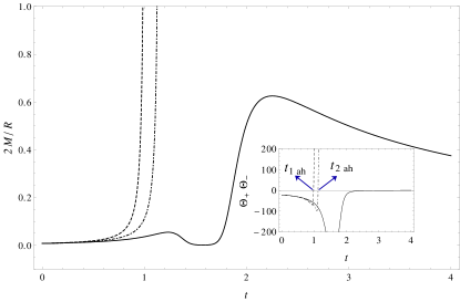
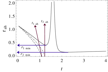
Figure 2: The time behavior of the Kretschmann invariant (upper panel), the ratio $2M/R$ (middle panel) and the apparent horizon curve (lower panel), for different values of deformation parameter, $\ell=-0.211$ (solid curve), $\ell=0.211$ (dashed curve), $\ell=0$ (dotted-dashed curve), $\beta=-3.2$ and $\alpha=1.1$. The inset shows the time behavior of the invariant $\Theta_{+}\Theta_{-}$, $\ell=-0.211$ (solid curve), $\ell=0$ (dotted-dashed curve) and $\ell=0.211$ (dashed curve). We have taken the initial values $\phi(t_{i})=1.98$, $\dot{\phi}(t_{i})=0.711$, $a(t_{i})=3$, $\dot{a}(t_{i})=-0.868$ and $\rho_{i}=0.2511$.

The behavior of the effective energy density and the time derivative of the Misner-Sharp energy is shown in Fig. 3 . The full curve shows that the effective energy density increases up to a local maximum value (point A), where $\dot{a}$ has reached its negative maximum value. This could be associated with the first inflection point $t_{{\rm 1inf}}$, as the star contracts in an accelerating way. As the decelerating regime begins, the collapse slows down and proceeds to momentarily to stop. The effective energy density decreases to a zero value at $t=t_{{\rm cr}}$, as if some mass loss took place, possibly caused by the appearance of negative pressure coming from phase-space deformation effects, i.e., energy escaping as this reverse in the dynamics takes place. Since trapped surfaces are failed to form, this flux of energy may be visible by external observers. Thus, a soft bounce occurs when the contracting phase transits to an expanding one at a specific value of the scale factor between the time interval $\Delta t_{{\rm b}}$ (point B in upper plot of Fig. 3; cf. Fig. 1). Subsequently, as the collapse turns into expansion, the effective energy density increases again to an absolute maximum (point C), possibly due to energy being regained; finally, it decreases asymptotically, as the star continues to expand without restriction. The energy density never blows up and the singularity that was produced in the undeformed case is avoided. This behavior may be interpreted as follows: the collapse proceeds for a while and then halts at the bouncing stage (cf. the behaviors of $\dot{a}$ and $\ddot{a}$), after which the star expands and intakes some mass that may have escaped. Finally, as it carries on expanding without regaining any more mass, the density decreases. We notice that the mentioned behavior is only for the solid line.

The lower panel in Fig. 3 suggests indeed this behavior at this period; hence the peak for point C. Furthermore, the negative zone in this figure shows the outward flux of energy occurring in the deceleration phase, i.e., from points A to B in Fig. 1. Therefore, the matching with a suitable exterior geometry, namely the generalized Vaidya spacetime, must be carried out, which describes an outgoing radiation. We note that since the star has internal pressure and is radiating, the Schwarzchild metric may no longer be a suitable spacetime to describe the exterior region. On the other hand, through the matching procedure, the interior solution can be extended to the exterior region and this may tell us whether the horizons form. Let us be more precise. The geometry outside a spherically symmetric radiating body is given by the generalized Vaidya metric as VaidyaM

$$ds_{{\rm out}}^{2}=-\left(1-\frac{2{\mathcal{M}}(u)}{r_{v}}\right)du^{2}-2dudr_{v}+r_{v}^{2}d\Omega^{2},$$ (49)

where $\textit{u}=t-r_{v}$ and ${\mathcal{M}}(u)$ being the retarded (exploding) null coordinate and the gravitational mass inside the sphere of radius $r_{v}$, respectively. The above metric is to be matched, by means of Isreal-Darmois junction conditions IS-DAR , to the internal geometry [cf. (2)] at the boundary of the star which is a timelike hypersurface given by $r=r_{\Sigma}$. We assume that the second fundamental form is continuous across the boundary; there is no surface stress-energy or surface tension at the boundary (see SETEN for more details). The induced metrics as we approach $\Sigma$ from the interior and exterior regions are given by, respectively

$$ds_{\Sigma_{{\rm in}}}^{2} = -dt^{2}+a^{2}(t)r_{\Sigma}^{2}d\Omega^{2},$$

$$ds_{\Sigma_{{\rm out}}}^{2} = -\left[\left(1-\frac{2{\mathcal{M}}(u)}{r_{v}}\right)\dot{u}^{2}+2\dot{u}\dot{r}_{v}\right]dt^{2}+r_{v}^{2}d\Omega^{2},$$

where $\dot{}\equiv d/dt$. Matching the induced metrics across $\Sigma$ we get

$$r_{v}(t)=r_{\Sigma}a(t),\leavevmode\nobreak\ \leavevmode\nobreak\ \leavevmode\nobreak\ \left(1-\frac{2{\mathcal{M}}(u)}{r_{v}}\right)\dot{u}^{2}+2\dot{u}\dot{r}_{v}=1.$$ (51)

Matching the extrinsic curvature components calculated from the interior and exterior geometries and after a straightforward but lengthy calculation, we get at the boundaryTrends-Bo

$$2{\mathcal{M}}|_{\Sigma}=r_{\Sigma}^{3}a\dot{a}^{2}=2M|_{\Sigma}.$$ (52)

Following Chinese , let us cast the exterior line element into dual-null form as

$$ds_{{\rm out}}^{2}=-2d\xi^{+}d\xi^{-}+r_{v}^{2}d\Omega^{2},$$ (53)

with the dual-null one-forms given by

$$d\xi^{+}=\frac{1}{2}du,\leavevmode\nobreak\ \leavevmode\nobreak\ \leavevmode\nobreak\ \leavevmode\nobreak\ \leavevmode\nobreak\ \leavevmode\nobreak\ d\xi^{-}=\left(1-\frac{2{\mathcal{M}}}{r_{v}}\right)du-2dr_{v}.$$ (54)

The corresponding radial null expansions are given by

$$\theta_{+}=\frac{2}{r_{v}}\left(1-\frac{2{\mathcal{M}}}{r_{v}}\right),\leavevmode\nobreak\ \leavevmode\nobreak\ \leavevmode\nobreak\ \theta_{-}=-\frac{1}{r_{v}}.$$ (55)

The dynamical horizon in the generalized Vaidya spacetime is located at $\theta_{+}=0$ or simply $2{\mathcal{M}}=r_{v}$, which lies on the boundary surface if $2M=R$. Then, from 52 we readily get

$$|\dot{a}|=\frac{1}{r_{\Sigma}},$$ (56)

which implies that once the collapse velocity reaches the value that satisfies the above equation, the dynamical horizon intersects the boundary of the star. Figure 4 shows the absolute value of the collapse velocity versus the scale factor. The horizontal arrows label different values of $|\dot{a}|$ for different boundary radii, as Eq. (56) dictates. There are two thresholds for the horizon formation, one in the collapse phase, which corresponds to $|\dot{a}_{{\rm 1max}}|=1/r_{1\Sigma}$, and the other one in the expanding phase which corresponds to $|\dot{a}_{{\rm 2max}}|=1/r_{2\Sigma}$. Thus, for $\ell<0$ (solid curve), the following considerations can be remarkable:

• The regularity condition demands that there must be no trapping of light at the initial epoch from which the collapse scenario begins. Thus there exists a maximum radius, namely, $r_{{\rm rg\Sigma}}$, so that if $r_{{\rm b}}=r_{{\rm rg\Sigma}}$ the regularity condition breaks down. Then, we could deduce that if the boundary surface is taken so that $r_{1\Sigma}<r_{{\rm b}}<r_{{\rm rg\Sigma}}$ or equivalently $|\dot{a}_{{\rm rg}}|<|\dot{a}|<|\dot{a}_{{\rm 1max}}|$, three horizons may appear (see the dashed arrow labeled as D, in Fig. 4); in the accelerated contracting regime, (from the initial configuration until point A or the first inflection point, see Fig. 1) as $|\dot{a}|$ increases, the first horizon forms to intersect the boundary until the time at which the decelerated contracting regime begins. After this time, $|\dot{a}|$ starts decreasing until getting vanished at the bounce, i.e., from point A to B. During this time interval where a decelerated contracting regime governs the collapse procedure, the horizon condition (56) is satisfied for the second time at an inner horizon. Contrary to the outer horizon, this one is situated in a modified regime where the weak energy condition (WEC) is effectively violated (due to the appearance of negative pressure) and $\ddot{a}>0$. As the collapse is replaced by a bounce and an accelerated expanding regime gets started, i.e., from points B to C, the condition (56) is fulfilled for the third time and a dynamical horizon intersects the matching surface.

• If $r_{2\Sigma}<r_{{\rm b}}<r_{1\Sigma}$ or equivalently $|\dot{a}_{{\rm 1max}}|<|\dot{a}|<|\dot{a}_{{\rm 2max}}|$, then no horizon may form in the exterior zone throughout the collapse regime (see the dashed arrow labeled as E, in figure 4). However, two dynamical horizons may still occur to meet the boundary; one in the accelerated expanding phase ($t_{{\rm cr}}<t<t_{{\rm 2inf}}$) and the other one in the decelerated expanding phase ($t>t_{{\rm 2inf}}$). Therefore, the collapse procedure that is replaced by a bouncing scenario may be covered by these horizons.

• Finally, if $r_{{\rm b}}<r_{2\Sigma}$ or equivalently $|\dot{a}|>|\dot{a}_{{\rm 2max}}|$, no horizon may occur in the exterior Vaidya region and the bounce is uncovered (see the dashed arrow labeled as F, in Fig. 4).

In contrast to the case $\ell<0$ for which $|\dot{a}|$ is bounded during the evolution of the setting, it grows boundlessly for $\ell>0$ and $\ell=0$ so that there cannot be found any threshold for the collapse velocity or any minimum radius for the boundary in order to avoid the formation of horizons. Thus as we approach the singularity, a dynamical horizon will always form to cover the singularity. In order to see whether the outward flux of energy can be visible to faraway observers, we assume that the energy flux as measured locally by an observer with a four-velocity vector $\zeta^{\mu}$ is given by LINSCHM

$$\sigma\equiv T_{\mu\nu}\zeta^{\mu}\zeta^{\nu}.$$ (57)

We consider only radially moving observers and define the radial velocity for such an observer as

$$v\equiv\zeta^{r_{v}}=\frac{dr_{v}}{dt}.$$ (58)

This follows then from $\zeta_{\mu}\zeta^{\mu}=-1$ and $\zeta^{\theta}=\zeta^{\phi}=0$

$$\frac{du}{dt}=\zeta^{u}=\frac{\eta-v}{\left(1-\frac{2{\mathcal{M}}(u)}{r_{v}}\right)}=\frac{1}{\eta+v},$$ (59)

where

$$\eta=\left(1+v^{2}-\frac{2{\mathcal{M}}(u)}{r_{v}}\right)^{-1}.$$ (60)

By calculating the nonvanishing component of Ricci tensor, i.e., $\left(R_{uu}=-\frac{2}{r_{v}^{2}}\frac{d{\mathcal{M}}}{du}\right)$ and using Eq. (57), we get the following expression for the energy flux $\sigma$, as

$$\sigma=-\frac{1}{(\eta+v)^{2}}\left(\frac{1}{4\pi r_{v}^{2}}\frac{d{\mathcal{M}}(u)}{du}\right).$$ (61)

The total luminosity for an observer with speed $v$ and the radius $r_{v}$ is given by LINSCHM

$$L(u)=4\pi r_{v}^{2}\sigma.$$ (62)

Substituting Eq. (61) into (62) we get

$$L(u)=-\frac{1}{(\eta+v)^{2}}\frac{d{\mathcal{M}}(u)}{du}.$$ (63)

Then, using Eq. (59) in Eq. (63), we can rewrite the luminosity, in terms of the interior mass function as

$$L(u)=-\frac{\dot{M}}{(\eta+v)}.$$ (64)

For an observer being at rest ($v=0$) at infinity ($r_{v}\rightarrow\leavevmode\nobreak\ \infty$), the total luminosity of the radiation can be obtained by taking the limit of (64) as

$$L_{\infty}(u)=-\dot{M}.$$ (65)

As we have described herein this paper, the negative pressure coming from phase-space deformation effects decelerates the collapse procedure until the bouncing time. Therefore, when the collapse enters the slow reacting regime, i.e., $t_{{\rm 1inf}}<t<t_{{\rm cr}}$, (see the lower plot in Fig. 1) the horizon is expected to shrink due to the modifications coming from phase-space deformation in the interior spacetime, which led to the violation of WEC (this allows the bounce to happen Trends-Bo ). Since $\dot{M}<0$ in this regime we may conclude that $L_{\infty}(u)\!\!\mid_{t_{{\rm 1inf}}<t<t_{{\rm cr}}}>0$; thus the radiation emanating from the bounce process may be possible to be detected by external observers. However, since $|\dot{a}|$ is bounded (for $\ell<0$), then, by suitable choice of the boundary surface $r=r_{\Sigma}$, the horizon formation is avoided. In such a situation, we have a regular matter configuration that initially collapses, reaches high densities and then disperses without the horizon formation.

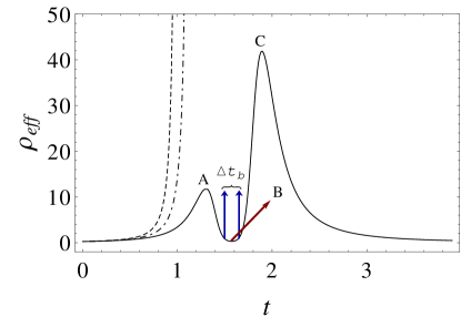
Figure 3: The time behavior of the effective energy density and $\dot{M}$ for different values of deformation parameter, $\ell=-0.211$ (solid curve), $\ell=0.211$ (dashed curve), $\ell=0$ (dotted-dashed curve) for $\beta=-3.2$ and $\alpha=1.1$. We have taken the initial values $\phi(t_{i})=1.98$, $\dot{\phi}(t_{i})=0.711$, $a(t_{i})=3$, $\dot{a}(t_{i})=-0.868$ and $\rho_{i}=0.2511$.

In Fig. 5 we have plotted the scale factor for different values of deformation parameter. It is seen that, as the absolute value of $\ell$ increases, the bouncing stage increases. This may be seen from the pressure originating from the deformation effects (cf. the upper plot of Fig. 9). The larger the value of $p_{d}$, the longer the time scale of the bounce. Let us briefly mention that although (12) remains unchanged under deformation, the time behavior of the kinetic energy of the scalar field in this equation is different.

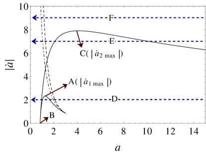
Figure 4: The behavior of absolute value of the collapse velocity in terms of the scale factor for different values of deformation parameter, $\ell=-0.211$ (solid curve), $\ell=0.211$ (dashed curve) and $\ell=0$ (dotted-dashed curve) for $\beta=-3.2$ and $\alpha=1.1$. The horizontal dashed arrows correspond to different values of $r_{{\rm b}}$, see the text for details. We have taken the initial values $\phi(t_{i})=1.98$, $\dot{\phi}(t_{i})=0.711$, $a(t_{i})=3$, $\dot{a}(t_{i})=-0.868$ and $\rho_{i}=0.2511$.

Figure 5: The time behavior of the scale factor for different values of deformation parameter, $\ell=-0.07385$ (solid curve), $\ell=-0.1266$ (dotted curve), $\ell=-0.19412$ (dashed curve), $\ell=-0.38402$ (dotted-dashed curve) for $\beta=-3.2$ and $\alpha=1.1$. We have taken the initial values $\phi(t_{i})=1.98$, $\dot{\phi}(t_{i})=0.711$, $a(t_{i})=3$, $\dot{a}(t_{i})=-0.868$ and $\rho_{i}=0.2511$.

Fig. 6  shows our numerical simulation for the scalar field and its kinetic energy. The full curve shows that the scalar field increases monotonically with a soft slope at the bouncing. The kinetic energy decreases after a local maximum as the collapse reaches the bouncing time, while regarding (22), the potential energy decreases too and cancels the kinetic energy. Therefore, the collapse rate vanishes and changes from a collapsing phase to a bouncing phase GJM12 . Such a transition can be better seen in the phase portrait of the collapse rate and effective energy density. As we see from Eq. (45) [or from (76)], there are two branches i.e., collapsing and expanding phases for negative and positive signs of the collapse rate, respectively. Thus, as the star initially begins to contract, the collapse rate approaches zero (see the left half-plane of Fig. 7), where the bounce appears at a finite scale factor and then starts to expand at later times, see right half-plane of Fig. 7. The dotted-dashed curve in Fig. 6  presents the situation in the absence of phase-space deformation, with the scalar field increasing boundlessly and the kinetic energy diverging to infinity. The dashed curve shows the behavior of these quantities for positive value of $\ell$ whereas we see the kinetic energy grows more rapidly than the case $\ell=0$.

For the collapsing matter clouds, it is usually required that the WEC be respected by the collapse configuration. In the collapse setting presented herein, WEC is given by $\rho_{{\rm eff}}\geq 0$ and $\rho_{{\rm eff}}+p_{{\rm eff}}\geq 0$. The first inequality holds for both undeformed and deformed configurations and the second one also remains valid for undeformed case. However, as Fig. 8 shows the second inequality holds only in the weak field regime, i.e., close to the initial configuration of the collapse setting, since the pressure appearing as phase-space deformation effects becomes dominant over the effective energy density at later stages. Such a crucial feature leads to the violation of WEC, which can be seen in several collapse settings where the effects of quantum gravity become prominent in strong field regimes DMQG . However the herein setting guarantees the positivity of the effective energy density.

Figure 6: The time behavior of the scalar field and its kinetic energy for different values of deformation parameter, $\ell=-0.211$ (solid curve), $\ell=0.211$ (dashed curve), $\ell=0$ (dotted-dashed curve) for $\beta=-3.2$ and $\alpha=1.1$. We have taken the initial values $\phi(t_{i})=1.98$, $\dot{\phi}(t_{i})=0.711$, $a(t_{i})=3$, $\dot{a}(t_{i})=-0.868$ and $\rho_{i}=0.2511$.

Figure 7: The phase-space of the collapse rate and effective energy density for $\ell=-0.211$, $\beta=-3.2$ and $\alpha=1.1$. We have taken the initial values $\phi(t_{i})=1.98$, $\dot{\phi}(t_{i})=0.711$, $a(t_{i})=3$, $\dot{a}(t_{i})=-0.868$ and $\rho_{i}=0.2511$.

Figure 8: The behavior of weak energy condition for different values of deformation parameter, $\ell=-0.211$ (solid curve), $\ell=0.211$ (dashed curve), $\ell=0$ (dotted-dashed curve) for $\beta=-3.2$, and $\alpha=1.1$. We have taken the initial values $\phi(t_{i})=1.98$, $\dot{\phi}(t_{i})=0.711$, $a(t_{i})=3$, $\dot{a}(t_{i})=-0.868$ and $\rho_{i}=0.2511$.

IV Conclusions

In this paper, concerning a scenario of gravitational collapse, we probed singularity formation (or the possibility of its removal) in the presence of a phase-space deformation within the canonical momenta sector. To be more precise, our matter content was described by the Lagrangian density of a scalar field minimally coupled to the spacetime curvature. The interior spacetime as taken as that of flat Friedmann-Lemaître-Robertson-Walker metric JG04 , JGS-LQ , BOJOetal . Thereby, by employing an Hamiltonian formalism, we explored the consequences of the dynamical deformation (35) in the phase-space.

The choice of such a type of deformation, whose particular form can be further discussed by means of a dimensional analysis, was motivated RFK11 . Additional arguments for it can be found also in RFK11 , namely with respect to the noncommutativity between the canonical momenta.

More concretely, the phase-space deformation emerges in the equations of motion by means of specific new terms, characterized by a parameter $\ell$. This could be taken either as positive or negative ($\ell=0$ representing the no deformation setting). The case $\ell>0$ leads us to an additional positive pressure effect, speeding up the collapse toward the singularity. Whereas, in the $\ell<0$ case, a negative pressure is present, inducing the collapse (that would have been toward a singularity) to be replaced by a nonsingular bounce.

It may be appropriate to compare the deformed equations with the corresponding ones when $\ell=0$. In the usual collapsing regime, as is seen from Eq. (14), the $\dot{\phi}$ term acts as antifriction throughout the collapse. From Eq. (47), we may intuitively consider that a negative value of a quantity associated to phase-space deformation parameter, would balance the antifriction term. In fact, it was precisely an additional negative pressure ($p_{d}$), induced from the phase-space deformation, that changed the collapsing picture: in the undeformed regime, for $\beta<-1$, trapped surfaces do form as Eq. (33) shows and thus the resulting singularity is covered, while in the deformed one (for $\ell<0$) trapped surfaces may be avoided till the time at which the bounce occurs, see the middle plot of Fig. 2 . Since trapped surfaces are failed to form, there may exist an outward flux of energy, due to which the effective mass reduces, see the $\dot{M}<0$ period in the lower plot of Fig. 3 . At later times, when the star begins an expanding phase, it absorbs the energy that has been escaping the collapsing phase. Thus, gravity becomes repulsive due to the presence of $p_{d}$. This provides the bouncing behavior and hence a singularity avoidance, depending thus on the deformation parameter. It is worth noting that the time scale of the bounce depends on the absolute magnitude of the deformation parameter.

Figure 9: Upper panel: The time behavior of the induced pressure originated from the phase-space deformation and the collapse velocity for $\ell=-0.211$. Middle panel: The time behavior of effective pressure, for different values of deformation parameter, $\ell=-0.211$ (solid curve), $\ell=0.211$ (dashed curve), $\ell=0$ (dotted-dashed curve) for $\beta=-3.2$ and $\alpha=1.1$. Lower panel: The time behavior of $p_{d}$ for $\ell=-0.211$ (solid curve), $\ell=0.211$ (dashed curve), $\ell=0$ (dotted-dashed curve), and $\beta=-3.2$. We have taken the initial values $\phi(t_{i})=1.98$, $\dot{\phi}(t_{i})=0.711$, $a(t_{i})=3$, $\dot{a}(t_{i})=-0.868$ and $\rho_{i}=0.2511$.

In summary, in the early stages of the collapse, as time advances, the velocity of the collapse becomes more and more negative; meanwhile the pressure $p_{d}$ that emerges from phase-space deformation effects comes into play, to prevent the collapsing phase to proceed. This pressure starts from a small negative value and progresses gradually to more negative values, thus ceasing the growth of the collapse velocity, up to a maximum negative value (see point A in Fig. 1). From then, the collapse continues but in a decelerating phase so that $p_{d}$ reaches its local maximum in negative direction (see the upper plot in Fig. 9). After that, $p_{d}$ proceeds, competing with gravitational attraction, until the time at which the collapse velocity becomes zero, where, during $\Delta t_{{\rm b}}$, the pressure $p_{d}$ stays for a while in its local minimum. Then, the collapse smoothly transforms to an accelerated expansion owing to this negative pressure, and this situation continues until that $p_{d}$ achieves its absolute maximum (negative value), where $\dot{a}$ and the effective energy density reach their maximum value. Finally, as the procedure enters a weak field regime, the deformation effects start to ease, so that the velocity of expansion and the effective energy density converge asymptotically. However, for positive values of the phase-space deformation parameter, it makes the last term in Eq. (47) behave as an antifriction term and prompts the collapse scenario to reach the singularity faster than the case in which the deformation effects are absent. The middle plot of Fig. 9  further shows that the effective pressure for $\ell<0$ begins from positive values, then turning to negative ones as the bounce occurs. For $\ell>0$ the effective pressure remains always positive and diverges. Indeed, the associated positive pressure adds to gravity and strengthens its attractiveness property, see dashed curve in the lower plot of Fig. 9. Let us further mention that, from Fig. (1), if we set the interval $\Delta t_{s}=t_{s}-t_{i}$ as the time that the collapse takes to hit the singularity, then the following inequality holds

$$\Delta t_{\ell^{+}}<\Delta t_{s}<\Delta t_{\ell^{-}},$$ (66)

where $\Delta t_{\ell^{+}}=\bar{t}_{s}-t_{i}$ is the time that the collapse scenario takes to reach the singularity at $t=\bar{t}_{s}$ (for $\ell>0$), and $\Delta t_{\ell^{-}}=t_{{\rm cr}}-t_{i}$ is the time that is taken up until the collapse transforms to a bounce. The fact is that for $\ell<0$, the collapse slows down due to the appearance of the negative pressure $p_{d}$, which prompts the collapse to turn into a bounce at the time $t_{{\rm cr}}>t_{s}$. Conversely, for $\ell>0$, the corresponding positive pressure causes the collapse to reach the singularity at an earlier time than the case $\ell=0$; hence $\bar{t}_{s}<t_{s}$.

Finally, we would like to point out that besides the setting presented here, there are various works in the literature on other bouncing scenarios. Among them we quote $f(R)$ theories in Palatini formalism FRPal , generalized teleparallel gravity theories TELL and in the presence of interacting spinning particles in the framework of Einstein-Cartan theory ECSPIN . The occurrence of bounces have been reported in spatially flat isotropic models in loop quantum cosmology for a massless scalar field LQCSFH , for different matter models LQCMA , and in the presence of anisotropy LQCANISO (see also LQCUP and references therein). In addition, models based on loop quantum gravity suggest that the singularity (that forms in the classical framework of gravitational collapse), can be regularized when the collapse scenario enters the Planckian regimes; semiclassical effects into the gravitational collapse of a homogeneous scalar field replace the singularity by a nonsingular bounce BOJOetal ; YJA . The same approach for a closed universe filled with a massive scalar field, which classically collapses to a singularity has been investigated in BIGC and it was shown that loop quantum effects in high curvature regimes led to a bouncing scenario, irrespective of the initial conditions. In the end, coordinate noncommutativity may also result in remarkable cosmological scenarios Octavio-COS as well as its role in curing the problems we face in describing the final fate of a radiating black hole, such as removing the curvature singularity being present in the commutative case Nicolini .

V Acknowledgments

One of us (S.M.M.R) is grateful for the support of Grant No. SFRH/BPD/82479/2011 from the Portuguese Agency Fundação para a Ciência e Tecnologia. This research work was supported by Grant No. CERN/FP/123618/2011. We would like to thank Nima Khosravi and Shahram Jalalzadeh for useful discussions and comments.

Appendix A Another (second) approach for deriving the equations of motion of sec. (III)

Here, we would like to apply another approach, which has been employed in the former investigations (see e.g. Refs. Other ,KS08 ), to derive the equations of motion associated to the deformed space of Sec. III. Let us start by introducing the following variables

$$\begin{cases}P^{\prime}_{\phi^{\prime}}\,=\,P_{\phi}-\ell a\phi^{3}\\ \phi^{\prime}(t)=\,\phi(t),\;N^{\prime}(t)=N(t)\\ a^{\prime}(t)\,=\,a(t),\;P^{\prime}_{a^{\prime}}=P_{a}.\end{cases}$$ (67)

We can easily show that the above variables satisfy the relation (35) if the unprimed variables satisfy the standard Poisson brackets. By employing the above transformations, the Hamiltonian (36) changes to

$${\mathcal{H}}_{0}^{{\rm nc}}={\mathcal{H}}_{0}-N\ell a^{-2}\phi^{3}P_{\phi}+\frac{1}{2}N\ell^{2}a^{-1}\phi^{6},$$ (68)

where $H_{0}$ is given by (3). In fact, by employing the transformation (67), the Hamiltonian ${\mathcal{H^{\prime}}}_{0}$ (as a function of the primed variables) has been replaced by ${\mathcal{H}}_{0}^{{\rm nc}}$, as a function of the unprimed variables. Finally, we write the Dirac Hamiltonian for the deformed scenario as

$${\mathcal{H}}^{{\rm nc}}={\mathcal{H}}_{0}^{{\rm nc}}+\lambda P_{N}.$$ (69)

The equations of motion with respect to the above Hamiltonian become

$$\dot{a}\!\! = \!\!\!\{a,{\mathcal{H}}^{{\rm nc}}\}=-\frac{1}{6}Na^{-1}P_{a},$$ (70)

$$\dot{P}_{a}\!\! = \!\!\!\{P_{a},{\mathcal{H}}^{{\rm nc}}\}=-\frac{1}{12}Na^{-2}P_{a}^{2}+\frac{3}{2}Na^{-4}P_{\phi}^{2}$$ (71)

$$- \!\!\!2N\ell a^{-3}\phi^{3}P_{\phi}+\frac{1}{2}N\ell^{2}a^{-2}\phi^{6}-3Na^{2}V(\phi),$$

$$\dot{\phi}\!\! = \!\!\!\{\phi,{\mathcal{H}}^{{\rm nc}}\}=Na^{-3}P_{\phi}-N\ell a^{-2}\phi^{3},$$ (72)

$$\dot{P}_{\phi}\!\! = \!\!\!\{P_{\phi},{\mathcal{H}}^{{\rm nc}}\}=3N\ell a^{-2}\phi^{2}P_{\phi}-3N\ell^{2}a^{-1}\phi^{5}$$ (73)

$$- Na^{3}\frac{dV(\phi)}{d\phi},$$

$$\dot{N}\!\! = \!\!\!\{N,{\mathcal{H}}^{{\rm nc}}\}=\lambda\,,$$ (74)

$$\dot{P}_{N}\!\! = \!\!\!\{P_{N},{\mathcal{H}}^{{\rm nc}}\}=\frac{1}{12}a^{-1}P_{a}^{2}-\frac{1}{2}a^{-3}P_{\phi}^{2}$$ (75)

$$+ \!\!\!\ell a^{-2}\phi^{3}P_{\phi}-\frac{1}{2}\ell^{2}a^{-1}\phi^{6}-a^{3}V(\phi),$$

where, to derive the above equations, we have used the ordinary (standard) Poisson brackets. However, instead of the standard Hamiltonian (4), the noncommutative/deformed Hamiltonian (69) has been employed. Therefore, we should mention that the unprimed variables in this section are perfectly different from their corresponding in Sec. II, and they were denoted by the present shapes (i.e., in unprimed forms) only for simplicity.

In the comoving gauge, it is straightforward to show that the equations of motion are given by

$$\left(\frac{\dot{a}}{a}\right)^{2}=\frac{1}{3}\left[\frac{1}{2}\dot{\phi}^{2}+V(\phi)\right]=\frac{1}{3}\rho_{{\rm eff}},$$ (76)

$$2\frac{\ddot{a}}{a}+\left(\frac{\dot{a}}{a}\right)^{2}\!\!\! = \!\!\!-\left[\frac{1}{2}\dot{\phi}^{2}-V(\phi)\right]-\frac{1}{3}\ell a^{-2}\phi^{3}\dot{\phi}$$ (77)

$$\equiv \!\!\!-(p+p_{{\rm d}})\equiv-p_{{\rm eff}},$$

$$\ddot{\phi}+3\left(\frac{\dot{a}}{a}\right)\dot{\phi}+\frac{dV(\phi)}{d\phi}+\ell\dot{a}\left(\frac{\phi}{a}\right)^{3}=0,$$ (78)

where $p_{{\rm d}}\equiv 1/3\ell a^{-2}\phi^{3}\dot{\phi}$.

In order to monitor the role of transformations (67) more vividly in this paper, we should mention a few comments regarding the primed and unprimed variables. The behavior of the unprimed variables in this section, and also in Sec. III, are not the same as the behavior of the corresponding ones in Sec. II. As mentioned several times, they reduce to their standard counterparts by letting $\ell=0$. In fact, in this paper, we have obtained the equations of motion by means of two different approaches and realized that these equations are perfectly equivalent. In fact, introducing relations such as (67), that can be seen in many investigations [see e.g. Other KS08 ], may just be an appropriate mathematical transformation, at least in our paper, to derive the equations of motion with a simpler manner. We should stress that the only way to recover the standard (commutative) results from the noncommutative ones is to set the deformation parameter equal to zero.

Appendix B About the equations of motion in Sec. III

The effects of phase-space deformation employed in this paper reveals itself as an additional pressure in Eq. (77) so that the conservation of the effective energy-momentum tensor Octavio-COS leads to the modified evolution equation for the scalar field. Let us take the derivative of the right- and left-hand side of Eq. (76), giving

$$\dot{\rho}_{{\rm eff}}=6H\dot{H}.$$ (79)

From Eqs. (76) and  (77), we have

$$\rho_{{\rm eff}}+p_{{\rm eff}}=2H^{2}-2\frac{\ddot{a}}{a}.$$ (80)

Applying Eqs. (79), (80) and $\dot{H}=\ddot{a}/a-H^{2}$, it provides

$$\dot{\rho}_{{\rm eff}}+3H\left(\rho_{{\rm eff}}+p_{{\rm eff}}\right)=0.$$ (81)

We now use the right-hand side and middle expression of Eq. (76) to obtain

$$\dot{\rho}_{{\rm eff}}=\dot{\phi}\ddot{\phi}+\dot{\phi}\frac{dV(\phi)}{d\phi}.$$ (82)

Again, using the right-hand side and middle expresions of Eqs. (76) and  (77), gives

$$3H\left(\rho_{{\rm eff}}+p_{{\rm eff}}\right)=3H\dot{\phi}\left(\dot{\phi}+\frac{1}{3}\ell a^{-2}\phi^{3}\right).$$ (83)

Adding the left- and right-hand sides of Eqs. (82) to  (83), it follows

$$\dot{\rho}_{{\rm eff}} +\leavevmode\nobreak\ 3H\left(\rho_{{\rm eff}}+p_{{\rm eff}}\right)$$

$$= \dot{\phi}\left(\ddot{\phi}+\frac{dV(\phi)}{d\phi}+3H\dot{\phi}+\ell\dot{a}a^{-3}\phi^{3}\right).$$

By assuming $\dot{\phi}\neq 0$, we can obtain

$$\ddot{\phi}+3\left(\frac{\dot{a}}{a}\right)\dot{\phi}+\frac{dV(\phi)}{d\phi}+\ell\dot{a}\left(\frac{\phi}{a}\right)^{3}=0.$$ (85)

Obviously, all of the explanations of this section are also valid for the primed variables of Sec. III.

References

- (1) V. P. Frolov and I. D. Novikov, Black Hole Physics: Basic Concepts and New Developments (Fundamental Theories of Physics (Springer, Berlin, 1998; P. S. Joshi, Global Aspects in Gravitation and Cosmology (Oxford University Press, Oxford, 1993).
- (2) S. W. Hawking & G. F. R. Ellis, The Large Scale Structure of spacetime, Cambridge: Cambridge University Press (1973).
- (3) M. Wyman, Phys. Rev. D 24 839 (1981).
- (4) B. C. Xanthopoulos and T. Zannias, Phys. Rev. D 40 2564 (1989).
- (5) D. Christodoulou, Comm. Pure Appl. Math. 44 339 (1991).
- (6) D. Christodoulou, Comm. Pure Appl. Math. 46 1131 (1993).
- (7) D. Christodoulou, Ann. Math. 140 607 (1994).
- (8) D. Christodoulou, Ann. Math. 149 183 (1999).
- (9) M. W. Choptuik, Phys. Rev. Lett. 70 9 (1993).
- (10) J. M. Martin-Garcia and C. Gundlach, Phys. Rev. D 68, 024011 (2003).
- (11) R. Giambò, Class. Quantum Grav. 22 2295 (2005).
- (12) C. Gundlach and J. M. Martin-Garcia, Living Rev. Rel. 10 5 (2007), arXiv:0711.4620 [gr-qc].
- (13) R. Goswami, P. S. Joshi, D. Malafarina, arXiv:1202.6218 [gr-qc] (2012).
- (14) C. Kiefer, B. Sandhoefer, arXiv:0804.0672 [gr-qc]; E. Greenwood, D. Stojkovic, JHEP 06 (2008) 042, arXiv:0802.4087 [gr-qc]; P. Hajicek, and C. Kiefer, Int. J. Mod. Phys. D 10 775 (2001), arXiv:/0107102 [gr-qc].
-
(15)
C. Kiefer, Quantum Gravity”. Second
edition (Oxford University Press, Oxford, 2007);
P. S. Joshi, Gravitational Collapse and spacetime Singularities’, Cambridge University Press (Cambridge, 2007). - (16) H. S. Snyder, Phys. Rev 71 38 (1947); Phys. Rev 72 68 (1947).
- (17) R. J. Szabo Phys. Rep 378 207 (2003), arXiv:hep-th/0109162 ; M. R. Douglas and N. A. Nekrasov Rev. Mod. Phys 73 977 (2001), arXiv:hep-th/0106048.
- (18) T. Banks, W. Fischler, S. H. Shenker and L. Susskind, Phys. Rev. D 55 5112 (1997), arXiv:hep-th/9610043; N. Seiberg and E. Witten , JHEP 09 (1999) 032, arXiv:hep-th/9908142; A. Connes, M. R. Douglas, and A. Schwarz, JHEP 02 (1998) 003, arXiv:hep-th/9711162.
- (19) S. Doplicher, K. Fredenhagen, J. E. Roberts, Phys. Lett. B 331 39 (1994); ibid, Commun. Math. Phys. 172 187 (1995).
- (20) E. M. C. Abreu, Albert C. R. Mendes, Wilson Oliveira and Adriano O. Zangirolami SIGMA 6 083 (2010), arXiv:1003.5322 [math-ph]; E. M. C. Abreu, M. J. Neves, arXiv:1108.5133 [hep-th]; ibid arXiv:1310.8352 [hep-th].
- (21) S . Minwalla, M. Van Raamsdonk and N. Seiberg, JHEP 02 (2000) 020, arXiv:hep-th/9912072.
- (22) S. M. Carroll, J. A. Harvey, V. A. Kostelecky, C. D. Lane, and T. Okamoto, Phys. Rev. Lett. 87 141601 (2001), arXiv:hep-th/0105082; C. E. Carlson, C. D. Carone, and R. F. Lebed, Phys. Lett. B 518 201 (2001), arXiv:hep-th/0107291; 549 337 (2002), arXiv:hep-th/0209077; A. Anisimov, T. Banks, M. Dine, and M. Graesser, Phys. Rev. D 65 085032 (2002), arXiv:hep-th/0106356; J. M. Carmona, J. L. Cortés, J. Gamboa, and F. Méndez, Phys. Lett. B 565 222 (2003), arXiv:hep-th/0207158.
- (23) I. Hinchliffe, N. Kersting and Y. L. Ma, Int. J. Mod. Phys. A 19 179 (2004), arxiv:hep-th/0205040; G. Amelino-Camelia, Living Rev. Rel. 16 5 (2013), arXiv:0806.0339 [gr-qc]; G. Amelino-Camelia, L. Doplicher, S. Nam, and Y.-S. Seo, Phys. Rev. D 67 085008 (2003), arXiv:hep-th/0109191; G. Amelino-Camelia, G. Mandanici, and K. Yoshida, JHEP 0401 (2004) 037, arXiv:hep-th/0209254; S. Ghosh, arXiv:1303.1256 [gr-qc].
- (24) D. J. Gross and N. A. Nekrasov, JHEP 10 (2000) 021, arXiv:hep-th/0007204; F. Lizzi, R. J. Szabo, and A. Zampini, JHEP 08 (2001) 032, arXiv:hep-th/0107115.
- (25) V. P. Nair and A. P. Polychronakos, Phys. Lett. B 505 267 (2001), arXiv:hep-th/0011172; J. Gamboa, M. Loewe and J. C. Rojas, Phys. Rev. D 64 067901 (2001), arXiv:hep-th/0010220; S. Bellucci, A. Nersessian and C. Sochichiu, Phys. Lett. B 522 345 (2001), arXiv:hep-th/0106138; R. Banerjee, Mod. Phys. Lett A 17 631 (2002), arXiv:hep-th/0106280; B. Muthukumar and P. Mitra, Phys. Rev. D 66 027701 (2002), arXiv:hep-th/0204149 ; S. Samanta, Mod. Phys. Lett. A 21 675 (2006), arXiv:hep-th/0510138; S. Gangopadhyay and F. G. Scholtz, arXiv:0812.3474 [math-ph].
- (26) M. Chaichian and M. M. Sheikh-Jabbari, Phys. Rev. Lett 86 2716 (2001), arXiv:hep-th/0010175; X. Calmet, Eur. Phys. J. C 41 269 (2005), arXiv:hep-th/0401097; Z. Guralnik R. Jackiw, Pi, S.-Y. and A. P. Polychronakos, Phys. Lett. B 517 450 (2001), arXiv:hep-th/0106044.
- (27) O. Bertolami, J. G. Rosa, C. M. L. de Aragao, P. Castorina and D. Zappala, Phys. Rev. D 72 025010 (2005), arXiv:hep-th/0505064; R. Banerjee, B. Dutta Roy and S. Samanta, Phys. Rev. D 74 045015 (2006), arXiv:hep-th/0605277; A. Saha, Phys. Rev. D 81 125002 (2010) arXiv:0803.3957 [hep-th]; S. Samanta, arXiv:0804.0172 [hep-th].
- (28) E. Di Grezia, G. Esposito, G. Miele, J. Phys. A 41 164063 (2008), arXiv:0707.3318 [gr-qc].
- (29) J. M. Romero and J. A. Santiago, Mod. Phys. Lett. A 20 781 (2005), arXiv:hep-th/0310266.
- (30) R. Brandenberger and P.-M. Ho, Phys. Rev. D 66 023517 (2002), arXiv:hep-th/0203119; Q.-G. Huang and M. Li, J. Cosmol. Astropart. Phys. 11 001 (2003), arXiv:0308458 [astro-ph]; JHEP 06 014 (2003), arXiv:hep-th/0304203; H. Kim, G. S. Lee, and Y. S. Myung, Mod. Phys. Lett. A 20 271 (2005), arXiv:hep-th/0402018; H. Kim, G. S. Lee, H. W. Lee, and Y. S. Myung, Phys. Rev. D 70 043521 (2004), arXiv:hep-th/0402198; Y. S. Myung, Phys. Lett. B 601 1 (2004), arXiv:hep-th/0407066; Dao-jun Liu and Xin-zhou Li, Phys. Rev. D 70 123504 (2004), arXiv:0402063 [astro-ph]; G. Calcagni, Phys. Rev. D 70 103525 (2004), arXiv:hep-th/0406006; Phys. Lett. B 606 177 (2005), arXiv:hep-th/0406057; Rong-Gen Cai, Phys. Lett. B 593 1 (2004), arXiv:hep-th/0403134; C.-S. Chu, B. R. Greene, and G. Shiu, Mod. Phys. Lett. A 16 2231 (2001), arXiv:hep-th/0010207; S. Tsujikawa, R. Maartens, and R. Brandenberger, Phys. Lett. B 574 141 (2003), arXiv:0308169 [astro-ph]; G. Calcagni and S. Tsujikawa, Phys. Rev. D 70 103514 (2004), arXiv:0407543 [astro-ph].
- (31) M. Maceda, J. Madore, P. Manousselis, and G. Zoupanos, Eur. Phys. J. C 36 529 (2004), arXiv:hep-th/0306136.
- (32) H. Garcia-Compean, O. Obregon, and C. Ramirez, Phys. Rev. Lett. 88, 161301 (2002), arXiv:hep-th/0107250.
- (33) G. D. Barbosa and N. Pinto–Neto, Phys. Rev. D 70 103512 (2004), arXiv:hep-th/0407111.
- (34) A. Bina, S. Jalalzadeh, A. Moslehi, Phys. Rev. D 81 023528 (2010), arXiv:1001.0861 [gr-qc]; A. Bina, K. Atazadeh, S. Jalalzadeh, Int. J. Theor. Phys. 47 1354 (2008), arXiv:0709.3623 [gr-qc]; S. Pramanik, S. Ghosh, arXiv:1301.4042 [hep-th].
- (35) R. J. Szabo, Class. Quant. Grav 23 R199 (2006), arxiv:hep-th/0606233; F. Muller-Hoissen, AIP Conf. Proc. 977 12 (2008), arXiv:0710.4418 [gr-qc].
- (36) A. Kempf and L. Lorenz, Phys. Rev. D 74 103517 (2006), arXiv:0609123 [gr-qc]; A. Ashoorioon, A. Kempf, and R. B. Mann, Phys. Rev. D 71 023503 (2005), arXiv:0410139 [astro-ph]; L. N. Chang, D. Minic, N. Okamura, and T. Takeuchi, Phys. Rev. D 65 125028 (2002), arXiv:hep-th/0201017; F. Brau and F. Buisseret, Phys. Rev. D 74 036002 (2006), arXiv:hep-th/0605183; J. Y. Bang and M. S. Berger, Phys. Rev. D 74 125012 (2006).
- (37) C. K. Zachos, D. B. Fairlie and T. L. Curtright (editors), Quantum Mechanics in phase-space, (World Scientific, Singapore, 2005).
- (38) C. Rovelli, Quantum Gravity, (Cambridge University Press, Cambridge, 2004).
- (39) T. Thiemann, Modern Canonical Quantum General Relativity, (Cambridge University Press, Cambridge, 2007).
- (40) M. B. Green, J.H. Schwarz and E. Witten, Superstring Theory, (Cambridge University Press, Cambridge, 1988).
- (41) J. Polchinski, String Theory, (Cambridge University Press, Cambridge, 1998).
- (42) H. Garcia–Compean, O. Obregon and C. Ramirez, Phys. Rev. Lett. 88 161301 (2002), arXiv:hep-th/0107250.
- (43) R. Goswami, and P. S. Joshi, arXiv:gr-qc/0410144 (2004).
- (44) R. Goswami, P. S. Joshi, P. Singh, Phys. Rev. Lett. 96 031302 (2006), arXiv:/0506129 [gr-qc].
- (45) M. Bojowald, R. Goswami, R. Maartens and P. Singh, Phys. Rev. Lett. 95 091302 (2005), arXiv:0503041 [gr-qc].
- (46) J. Plebański and A. Krasiński, An Introduction to General Relativity and Cosmology, Cambridge University Press, Cam-bridge (2006).
- (47) S. Hayward, Phys. Rev. D 49 6467 (1994), arXiv:9303006[gr-qc]; ibid, Phys. Rev. D 53 1938 (1996), arXiv:9408002 [gr-qc].
- (48) C. W. Misner and D. H. Sharp, Phys. Rev. 136 B571 (1964); S. A. Hayward, Phys. Rev. D 49 831 (1994), arXiv:9303030 [gr-qc].
- (49) J. C. Lopez-Dominguez, O. Obregon, C. Ramirez and M. Sabido, Phys. Rev. D 74 084024 (2006), arXiv:hep-th/0607002.
- (50) N. Khosravi, S. Jalalzadeh and H. R. Sepangi, JHEP 01 134 (2006), arXiv:hep-th/0601116; B. Vakili, P. Pedram, S. Jalalzadeh, Phys. Lett. B 687 119 (2010), arXiv:1003.1194 [gr-qc].
- (51) J. Lukierski, A. Nowicki, H. Ruegg and V. N. Tolstoy, Phys. Lett. B 264 331 (1991); J. Lukierski, A. Nowicki and H. Ruegg, Phys. Lett. B 293 344 (1992); J. Lukierski and H. Ruegg, Phys. Lett. B 329 189 (1994) arXiv:hep-th/9310117; P. Kosinski, P. Maslanka, arXiv:hep-th/9411033; A. Sitarz, Phys. Lett. B 349 42 (1995), arXiv:hep-th/9409014; P. Kosinski, J. Lukierski and P. Maslanka, Phys. Rev. D 62 025004 (2000) arXiv:hep-th/9902037; P. Kosinski, J. Lukierski and P. Maslanka, Czech. J. Phys. 50 1283 (2000), arXiv:hep-th/0009120; P. Kosinski, P. Maslanka, J. Lukierski and A. Sitarz, arXiv:hep-th/0307038; S. Meljanac, M. Stojic, Eur. Phys. J. C 47 531 (2006), arXiv:hep-th/0605133; S. K.-Juric, S. Meljanac, M. Stojic, Eur. Phys. J. C 51 229 (2007), arXiv:hep-th/0702215; L. Moller, JHEP 0512 029 (2005) arXiv:hep-th/0409128; H. Grosse and M. Wohlgenannt, Nucl. Phys. B 748 473 (2006) arXiv:hep-th/0507030; A. Agostini, G. Amelino-Camelia, M. Arzano and F. D’Andrea, arXiv:hep-th/0407227; A. Agostini, G. Amelino-Camelia, M. Arzano, A. Marciano and R. A. Tacchi, Mod. Phys. Lett. A 22 1779 (2007) arXiv:hep-th/0607221; M. Arzano and A. Marciano, Phys. Rev. D 75 081701 (2007), arXiv:hep-th/0701268; L. Freidel, J. Kowalski-Glikman and S. Nowak Phys. Lett. B 648 70 (2007), arXiv:hep-th/0612170; A. Agostini, F. Lizzi and A. Zampini, Mod. Phys. Lett. A 17 2105 (2002), arXiv:hep-th/0209174.
- (52) G. Amelino-Camelia, L. Smolin and A. Starodubtsev, Class. Quant. Grav. 21 3095 (2004) arXiv:hep-th/0306134; L. Freidel, J. Kowalski-Glikman and L. Smolin, Phys. Rev. D 69 044001 (2004) arXiv:hep-th/0307085.
- (53) G. Amelino-Camelia, Phys. Lett. B 510 255 (2001), arXiv:hep-th/0012238.
- (54) G. Amelino-Camelia, Int. J. Mod. Phys. D 11 1643 (2002).
- (55) J. Magueijo and L. Smolin, Phys. Rev. Lett. 88 190403 (2002), arXiv:hep-th/0112090.
- (56) G. Amelino.-Camelia Int. J. Mod. Phys. D 11 35 (2002), arXiv:0012051 [gr-qc]; J. Magueijo and L. Smolin, Phys. Rev. D 67 044017 (2003), arXiv:0207085 [gr-qc]; J. Kowalski-Glikman, Lect. Notes Phys. 669 131 (2005), arXiv:hep-th/0405273; S. Ghosh and P. Pal, Phys. Rev. D 75 105021 (2007), arXiv:hep-th/0702159.
- (57) J. Kowalski-Glikman, Phys. Lett. A 299 454 (2002), arXiv:hep-th/0111110; J. Lukierski, H. Ruegg and W. J. Zakrzewski, Ann. Phys. 243 90 (1995), arXiv:hep-th/9312153; S. Majid and H Ruegg Phys. Lett. B 334 348 (1994), arXiv:hep-th/9405107.
- (58) J. M. Romero, J. D. Vergara and J. A. Santiago, Phys. Rev. D 75 065008 (2007), arXiv:hep-th/0702113.
- (59) N. R. Bruno, G. Amelino-Camelia and J. Kowalski-Glikman, Phys. Lett. B 522 133 (2001), arXiv:hep-th/0107039.
- (60) N. Khosravi and H. R. Sepangi, Phys. Lett. A 372 3356 (2008), arXiv:0802.0767 [gr-qc].
- (61) W. Guzman, M. Sabido and J. Socorro, Phys. Lett. B 697 271 (2011), arXiv:0812.4251 [gr-qc].
- (62) S. M. M. Rasouli, M. Farhoudi and N. Khosravi, Gen. Relativ. Gravit. 43 2895 (2011), arXiv:1006.5893 [gr-qc].
- (63) N. Khosravi, H. R. Sepangi and M. M. Sheikh-Jabbari, Phys. Lett. B 647 219 (2007), arXiv:hep-th/0611236.
- (64) J. Magueijo, T. G. Zlosnik, T. W. B. Kibble, Phys. Rev. D 87 063504 (2013), arXiv:1212.0585 [gr-qc].
- (65) P. C. Vaidya, Proc. Indian Acad. Sci. A 33 264 (1951); Reprinted, Gen. Rel. Grav. 31 119 (1999); W. B. Bonnor, A. K. G. de Oliveira and N. O. Santos, Phys. Rep. 181 269 (1989); P. S. Joshi and I. H. Dwivedi, Class. Quant. Grav. 16 41 (1999), arXiv:9804075 [gr-qc]; A. Wang and Y. Wu, Gen. Rel. Grav. 31 107 (1999), arXiv:9803038 [gr-qc].
- (66) W. Israel Nuovo Cimento B, 44 1 (1966); ibid, Nuovo Cimento B 48 463 (1967).
- (67) K. Lake, in Vth Brazilian school of cosmology and gravitation edited b M. Novello (World Scientific, Singapore, (1987); P. Musgrave and K. Lake, Class. Quantum Grav. 13 1885 (1996), arXiv:9510052 [gr-qc]; ibid, Class. Quantum Grav. 14 1285 (1997).
- (68) M. Bojowald, “Trends in Quantum Gravity Rsearch ,” D. C. Moore (editor), Nova Science Publishers, Inc. (2006).
- (69) Ji-Rong Ren and Ran Li, Mod. Phys. Lett. A 23 3265 (2008), arXiv:0705.4339 [gr-qc].
- (70) R. W. Lindquist, R. A. Schwartz, and C. W. Misner, Phys. Rev. 137 1364B (1965).
- (71) G. M. Hossain, Class. Quant. Grav. 22 2653 (2005), arXiv:0503065 [gr-qc]; C. Bambi, D. Malafarina, L. Modesto, Phys. Rev. D 88 044009 (2013), arXiv:1305.4790 [gr-qc].
- (72) C. Barragan, G. J. Olmo and H. Sanchis-Alepuz, Phys. Rev. D 80 024016 (2009), arXiv:0907.0318 [gr-qc].
- (73) Yi-Fu Cai, Shih-Hung Chen, J. B. Dent, S. Dutta and E. N. Saridakis, Class. Quantum Grav. 28 215011 (2011), arXiv:1104.4349 [gr-qc].
- (74) M. Gasperini, Gen. Relativ. Gravit. 30 1703 (1998), arXiv:9805060 [gr-qc]; S. D. Brechet, M. P. Hobson, A. N. Lasenby, Class. Quantum Grav. 25 245016 (2008), arXiv:0807.2523 [gr-qc]; N. Poplawski, Phys. Rev. D 85 107502 (2012), arXiv:1111.4595 [gr-qc]; N. Poplawski, Gen. Relativ. Gravit. 44 1007 (2012), arXiv:1105.6127 [astro-ph.CO].
- (75) A. Ashtekar, T. Pawlowski and P. Singh, Phys. Rev. Lett. 96 141301 (2006), arXiv:0602086 [gr-qc]; ibid, Phys. Rev. D 73 124038 (2006), arXiv:0604013 [gr-qc]; ibid, Phys. Rev. D 74 084003 (2006), arXiv:0607039 [gr-qc].
- (76) A. Ashtekar, T. Pawlowski, P. Singh and K. Vandersloot, Phys. Rev. D 75 0240035 (2007), arXiv:0612104 [gr-qc]; A. Ashtekar, A. Corichi and P. Singh, Phys. Rev. D 77 024046 (2008), arXiv:0710.3565 [gr-qc]; K . Vandersloot, Phys. Rev. D 75 023523 (2007), arXiv:0612070 [gr-qc]; L. Szulc, Class. Quantum. Grav. 24 6191 (2007), arXiv:0707.1816 [gr-qc]; E . Bentivegna and T. Pawlowski, Phys. Rev. D 77 124025 (2008), arXiv:0803.4446 [gr-qc]; W. Kaminski and T. Pawlowski, Phys. Rev. D 81 024014 (2010), arXiv:0912.0162 [gr-qc]; T. Pawlowski, A. Ashtekar, Phys. Rev. D 85 064001 (2012), arXiv:1112.0360 [gr-qc].
- (77) A. Ashtekar and E. Wilson-Ewing, Phys. Rev. D 79 083535 (2009), arXiv:0903.3397 [gr-qc]; ibid Phys. Rev. D 80 123532 (2009), arXiv:0910.1278 [gr-qc]; E. Wilson-Ewing, Phys. Rev. D 82 043508 (2010), arXiv:1005.5565 [gr-qc]; M. Martin-Benito, G. A. Mena Marugan and T. Pawlowski, Phys. Rev. D 78 064008 (2008), arXiv:0804.3157 [gr-qc]; ibid Phys. Rev. D 80 084038 (2009), arXiv:0906.3751 [gr-qc].
- (78) A. Ashtekar and P. Singh, Class. Quantum. Grav. 28 213001 (2011), arXiv:1108.0893 [gr-qc].
- (79) Y. Tavakoli, J. Marto, A. Dapor, arXiv:1303.6157 [gr-qc].
- (80) P. Singh, A. Toporensky, Phys. Rev. D 69 104008 (2004), arXiv:0312110 [gr-qc].
- (81) O. Obregon and I. Quiros, Phys. Rev. D 84 044005 (2011), arXiv:1011.3896 [gr-qc].
- (82) P. Nicolini, A. Smailagic and E. Spallucci, Phys. Lett. B 632 547 (2006), arXiv:0510112 [gr-qc]; P. Nicolini and E. Spallucci, Class. Quant. Grav. 27 015010 (2010), arXiv:0902.4654 [gr-qc]; E. Spallucci, A. Smailagic and Piero Nicolini, Phys. Lett. B 670 449 (2009), arXiv:0801.3519[hep-th]; P. Nicolini, A. Smailagic and E. Spallucci, ESA Spec. Publ. 637 11.1 (2006), arXiv:hep-th/0507226.
- (83) N. Khosravi, H. R. Sepangi, B. Vakili, Gen. Rel. Grav. 42 1081 (2010), arXiv:0909.2487 [gr-qc]; N. Khosravi, H. R. Sepangi, JCAP 0804:011 (2008), arXiv:0803.1714 [gr-qc], N. Khosravi, S. Jalalzadeh, H. R. Sepangi, JHEP0601:134 (2006), arXiv:hep-th/0601116; B. Vakili, N. Khosravi, H. R. Sepangi, Class. Quant. Grav. 24 931 (2007), arXiv:0701075 [gr-qc]; G. D. Barbosa, Phys. Rev. D 71 (2005) 063511, arXiv:hep-th/0408071.