The vector resonance triplet with the direct coupling to the third quark generation

Abstract

The effective Lagrangian with scalar and vector resonances that might result from new strong physics beyond the SM is formulated and studied. In particular, the scalar resonance representing the recently discovered 125-GeV boson is complemented with the $SU(2)_{L+R}$ triplet of hypothetical vector resonances. Motivated by experimental and theoretical considerations, the vector resonance is allowed to couple directly to the third quark generation only. The coupling is chiral-dependent and the interaction of the right top quark can differ from that of the right bottom quark. To estimate the applicability range of the effective Lagrangian the unitarity of the gauge boson scattering amplitudes is analyzed. The experimental fits and limits on the free parameters of the vector resonance triplet are investigated.

1 Introduction

The ATLAS and CMS announcements of the 125-GeV boson discovery 125GeVBosonDiscovery have provided major contribution towards finding the solution of the puzzle about the mechanism of electroweak symmetry breaking (ESB). The recent data revelations and analyses Moriond2013 strongly suggest that the observed 125-GeV boson is a Higgs-like particle with a tight relationship with the ESB mechanism. Nevertheless, the question about the true nature of the mechanism, and thus about physics beyond the Standard model (SM), remains unsolved. While the observed properties of the discovered boson are compatible with the SM Higgs boson hypothesis EllisYou ; HiggsAtLast ; NBlikeSMhiggs ; GlobalSMfit , at the same time they are compatible with some alternative extensions of the SM CapabilityOfMeasurements .

From a theoretical point of view, the alternatives to the SM Higgs get some preferences due to the naturalness argument. The extensions of the SM still in the game include theories where electroweak symmetry is broken by new strong interactions, like in Technicolor TC ; ETC ; WalkingTC ; TopcolorTC .

Most studies aimed at the evaluation of the impact of the new discovery on the alternatives theories assume the boson has a spin zero. This assumption gets a growing experimental support as more LHC data is being processed. Of course, at the same time it disfavors strongly-interacting theories without a light scalar field and calls for theories with a light composite strongly-interacting Higgs CompositeScalar-old ; CHsketch ; CompositeScalar ; HiggsLag ; CompositeScalar-GGduality ; alternatives of a proper mass.

A feverish activity in building effective descriptions and identifying possible underlying theories is taking place on the theoretical front nowadays. The focus lies in the modeling, parameterizing, and fitting the 125-GeV Higgs-like boson sector of candidate theories (see, e.g., ContinoEffLagrForLightHiggs ). Effectively, the Higgs-like boson can be described as a stand-alone singlet added to the non-linear sigma model of the Nambu–Goldstone bosons. This is the most model-independent approach, but with the least predictive power. Alternatively, the Higgs-like scalar can be made a member of a multiplet of the symmetry of the strong sector HiggsInMultiplet . The latter approach results in additional experimentally testable restrictions on free parameters of the model. At the same time, it can provide a mechanism for keeping the scalar resonance light.

Following theoretical arguments, as well as the example of QCD, it seems reasonable to expect that beside the composite scalar the new strong interactions would also produce bound states of higher spins. A natural candidate to look for is the vector $SU(2)$ triplet resonance. From another point of view, if the composite Higgs couplings differ from the SM ones, as is usually the case in strongly interacting theories, the Higgs alone will fail to unitarize the $VV$ $(V=W^{\pm},Z)$ scattering amplitudes. Then, additional resonances are required to tame the unitarity.

In this paper, we study the effective Lagrangian where beside the 125-GeV scalar resonance — an $SU(2)_{L+R}$ singlet complementing the non-linear triplet of the Nambu–Goldstone bosons — the $SU(2)_{L+R}$ triplet of vector resonances is explicitly present. It fits the situation when the global $SU(2)_{L}\times SU(2)_{R}$ symmetry is broken down to $SU(2)_{L+R}$. As far as the vector resonance sector is concerned, the vector triplet is introduced as a gauge field via the hidden local symmetry approach HLS . Because of this, the vector resonance mixes with the EW gauge bosons, which results in appearance of indirect couplings of the vector resonance with all SM fermions. Besides, the direct couplings of the vector resonance triplet to the SM fermions are also allowed by the Lagrangian symmetry. Regarding the direct couplings we opt for a special setup inspired by the speculations about an extraordinary role of the top quark (or the third quark generation) in new strong physics: we admit direct couplings of the new triplet to no other SM fermions, but the top and bottom quarks only. Finally, the symmetry allowed interaction terms between the scalar and vector resonances are also present.

In the strong scenario, the direct couplings between the SM fermions and the vector resonance can depend on the degree of compositeness of a given fermion as well as on symmetry group representations the fermions are organized into. In principle, the degree of compositeness of the SM fermions can vary for different flavors and chirality. Theories that can be related to our effective description include 2-site deconstructed models, purely 4-dimensional multi-site models, and composite Higgs models CompositeScalar-GGduality ; HiggsInMultiplet ; ContinoResonancesInCmpHiggs ; Sundrum ; DeCurtis ; PanicoPrivate . All these models predict the existence of resonances of higher spins, including the vectorial ones. The idea of partial compositeness that appears in some of these models could justify the exclusivity of the third quark direct couplings to the vector resonances in our effective Lagrangian.

The couplings of the hypothetical vector resonance to light fermions are tightly restricted by the existing measurements from the LEP, SLC, and Tevatron experiments. Thus, it is reasonable to neglect them also from the experimental point of view. The direct coupling of the vector resonance to the bottom quark is also restricted by the experiments through the measurement of the $Zbb$ vertex, at least. In our effective Lagrangian, the influence of this restriction on the direct interaction with the top quark has been weakened by the splitting of the interaction with the right top and bottom quark.

As far as the direct LHC bottom limits on the vector resonance masses are concerned they are strongly model-dependent. In general, it can be said that considering the partial compositeness for the third quark generation only admits the limits to be as low as 300 GeV, or even less, for certain values of the Higgs-like boson couplings CHsketch . The most restrictive bottom limit is obtained when no compositeness of the SM fermions is assumed; it is slightly below $1\;\mathrm{TeV}$.

In this paper, we study the unitarity constraints and the best fits of the vector resonance free parameters to the existing data. We perform the best-fit analysis under the simplifying assumption that the scalar resonance couplings are the SM ones. It should serve as an approximation of the situation allowed by the experiment when the actual scalar couplings do not differ too much from the SM ones. In setting constraints on the vector resonance couplings the published LHC analyses cannot compete with the low-energy measurements yet. Therefore we focus on the low-energy data when calculating the limits. Our analysis have been performed as a multi-observable $\chi^{2}$-fit taking into account the correlations among the observables used. The list of fitted observables is comprised of $\epsilon_{1}$, $\epsilon_{2}$, $\epsilon_{3}$, $\Gamma_{b}(Z\rightarrow b\bar{b}+X)$, and BR$(B\rightarrow X_{s}\gamma)$. Throughout the analysis the mass of the considered vector triplet assumes TeV values.

This paper is organized as follows. In Section 2 we introduce our effective Lagrangian. In Section 3 the tree-level unitarity limits for the longitudinal electroweak gauge boson scattering as function of the scalar and vector resonance parameters are calculated and discussed. Section 4 is devoted to the low-energy analysis of the vector resonance couplings. Section 5 contains our conclusions followed by appendices.

2 The effective Lagrangian

We introduce the $SU(2)_{L+R}$ triplet vector resonance to the usual $SU(2)_{L}\times SU(2)_{R}\rightarrow SU(2)_{L+R}$ effective Lagrangian with the non-linearly transforming $SU(2)_{L+R}$ triplet of the would-be Nambu–Goldstone bosons augmented with the $SU(2)_{L+R}$ singlet scalar resonance. The vector triplet is brought in as a gauge field via the hidden local symmetry (HLS) approach HLS . The effective Lagrangian is built to respect the global $SU(2)_{L}\times SU(2)_{R}\times U(1)_{B-L}\times SU(2)_{HLS}$ symmetry of which the $SU(2)_{L}\times U(1)_{Y}\times SU(2)_{HLS}$ subgroup is also a local symmetry. The $SU(2)_{HLS}$ symmetry is an auxiliary gauge symmetry invoked to accommodate the $SU(2)$ triplet of vector resonances. Beside the scalar singlet and the vector triplet, the effective Lagrangian is built out of the SM fields only.

Our effective Lagrangian can be split in three terms

$${\cal L}={\cal L}_{\mathrm{GB}}+{\cal L}_{\mathrm{ESB}}+{\cal L}_{\mathrm{ferm}},$$ (1)

where ${\cal L}_{\mathrm{GB}}$ describes the gauge boson sector including the $SU(2)_{\mathrm{HLS}}$ triplet, ${\cal L}_{\mathrm{ESB}}$ is the scalar sector responsible for spontaneous breaking of the electroweak and hidden local symmetries, and ${\cal L}_{\mathrm{ferm}}$ is the fermion Lagrangian of the model.

Beside the SM gauge fields $W_{\mu}^{a}(x)$ and $B_{\mu}(x)$, the $SU(2)_{\mathrm{HLS}}$ gauge triplet $\vec{V}_{\mu}=(V_{\mu}^{1},V_{\mu}^{2},V_{\mu}^{3})$ represents hypothetical neutral and charged vector resonances of a new strong sector. Under the $[SU(2)_{L}\times SU(2)_{R}]^{\mathrm{glob}}\times SU(2)_{\mathrm{HLS}}^{\mathrm{loc}}$ group the triplet transforms as

$$\mbox{\boldmath$V$}_{\mu}\rightarrow h^{\dagger}\mbox{\boldmath$V$}_{\mu}h+h^{\dagger}\partial_{\mu}h,$$ (2)

where $h(x)\in SU(2)_{\mathrm{HLS}}^{\mathrm{loc}}$ and $\mbox{\boldmath$V$}_{\mu}=i\frac{g^{\prime\prime}}{2}V_{\mu}^{a}\tau^{a}$. The $2\times 2$ matrices $\vec{\tau}=(\tau^{1},\tau^{2},\tau^{3})$ are the $SU(2)$ generators.

The ESB sector contains six unphysical real scalar fields, would-be Goldstone bosons of the model’s spontaneous symmetry breaking. The six real scalar fields $\varphi_{L}^{a}(x),\varphi_{R}^{a}(x),\;a=1,2,3$, are introduced as parameters of the $SU(2)_{L}\times SU(2)_{R}$ group elements in the exp-form $\xi(\vec{\varphi}_{L,R})=\exp(i\vec{\varphi}_{L,R}\vec{\tau}/v)\in SU(2)_{L,R}$ where $\vec{\varphi}=(\varphi^{1},\varphi^{2},\varphi^{3})$.

In the ESB sector the would-be Goldstone bosons couple to the gauge bosons $W_{\mu}^{a}$, $B_{\mu}$, $V_{\mu}^{a}$, and to the 125-GeV scalar resonance $h(x)$ obeying $[SU(2)_{L}\times U(1)_{Y}\times SU(2)_{\mathrm{HLS}}]^{\mathrm{loc}}$ symmetry requirements. Thus,

$${\cal L}_{\mathrm{ESB}} = \frac{1}{2}\partial_{\mu}h\,\partial^{\mu}h-\frac{1}{2}M_{h}^{2}h^{2}$$ (3)

$$-v^{2}\left[\mbox{Tr}\left(\bar{\omega}_{\mu}^{\perp}\right)^{2}+\alpha\;\mbox{Tr}\left(\bar{\omega}_{\mu}^{\parallel}\right)^{2}\right]$$

$$\phantom{-}\;\times\,(1+2a\frac{h}{v}+a^{\prime}\frac{h^{2}}{v^{2}}+\ldots),$$

where $\alpha$, $a,a^{\prime},\ldots$ are free parameters, $M_{h}=125\;\mathrm{GeV}$, and $\bar{\omega}_{\mu}^{\parallel,\perp}$ are, respectively, $SU(2)_{L-R}$ and $SU(2)_{L+R}$ projections of the gauged Maurer–Cartan 1-form,

$$\bar{\omega}_{\mu}^{\parallel} = \omega_{\mu}^{\parallel}+\frac{1}{2}\left(\xi_{L}^{\dagger}\mbox{\boldmath$W$}_{\mu}\xi_{L}+\xi_{R}^{\dagger}\mbox{\boldmath$B$}_{\mu}\xi_{R}\right)-\mbox{\boldmath$V$}_{\mu},$$ (4)

$$\bar{\omega}_{\mu}^{\perp} = \omega_{\mu}^{\perp}+\frac{1}{2}\left(\xi_{L}^{\dagger}\mbox{\boldmath$W$}_{\mu}\xi_{L}-\xi_{R}^{\dagger}\mbox{\boldmath$B$}_{\mu}\xi_{R}\right),$$ (5)

where $\omega_{\mu}^{\parallel,\perp}=(\xi_{L}^{\dagger}\partial_{\mu}\xi_{L}\pm\xi_{R}^{\dagger}\partial_{\mu}\xi_{R})/2$. When $a=a^{\prime}=1$ and all other $a$’s are zeros, the scalar resonance imitates the SM Higgs boson.

The masses of the vector triplet are set by the scale $v$ and depend on the three gauge couplings $g,g^{\prime},g^{\prime\prime}$, and the free parameter $\alpha$. In the limit when $g$ and $g^{\prime}$ are negligible compared to $g^{\prime\prime}$, the masses of the neutral and charged resonances are degenerate, $M_{V}=\sqrt{\alpha}g^{\prime\prime}v/2$. If higher order corrections in $g/g^{\prime\prime}$ are admitted, a tiny mass splitting occurs such that $M_{V^{0}}>M_{V^{\pm}}$ tBESS .

As far as the fermion sector is concerned no new fermions beyond the SM have been introduced in our Lagrangian. The fermion sector of the Lagrangian can be divided into three parts

$${\cal L}_{\mathrm{ferm}}={\cal L}_{\mathrm{ferm}}^{\mathrm{SM}}+{\cal L}_{\mathrm{ferm}}^{\mathrm{scalar}}+{\cal L}_{(t,b)}^{\mathrm{tBESS}},$$ (6)

where ${\cal L}_{\mathrm{ferm}}^{\mathrm{SM}}$ contains the SM interactions of fermions with the electroweak gauge bosons, ${\cal L}_{\mathrm{ferm}}^{\mathrm{scalar}}$ is about the interactions of the fermions with scalar fields and includes the fermion masses, and ${\cal L}_{(t,b)}^{\mathrm{tBESS}}$ describes the third quark generation direct interactions with the vector resonance. In addition, it contains symmetry allowed non-SM interactions of the third quark generation with the EW gauge bosons.

The first term of (6) is identical to its SM counterpart. Namely,

$${\cal L}_{\mathrm{ferm}}^{\mathrm{SM}}=\sum_{\forall\psi}\left[I_{c}^{L}(\psi_{L})+I_{c}^{R}(\psi_{R})\right],$$ (7)

where $\psi$ denotes the usual $SU(2)$ doublets of SM fermions and the sum runs through them. The invariants $I_{c}^{L,R}$ read

$$I_{c}^{L}(\psi_{L}) = i\bar{\psi}_{L}(\!\not{\!\mbox{\boldmath$\partial$}}+\!\not{\!\!\mbox{\boldmath$W$}}+\!\not{\!\!\mbox{\boldmath$B$}})\psi_{L},$$ (8)

$$I_{c}^{R}(\psi_{R}) = i\bar{\psi}_{R}(\!\not{\!\mbox{\boldmath$\partial$}}+\!\not{\!\!\mbox{\boldmath$B$}})\psi_{R}.$$ (9)

The second term of the Lagrangian (6) reads

$${\cal L}_{\mathrm{ferm}}^{\mathrm{scalar}}=-\sum_{i}I_{\mathrm{mass}}(\psi^{i})\,(1+c_{i}\frac{h}{v}+c_{i}^{\prime}\frac{h^{2}}{v^{2}}+\ldots),$$ (10)

where $c_{i},c_{i}^{\prime},\ldots$ are free parameters, and

$$I_{\mathrm{mass}}(\psi^{i})=\bar{\psi}_{L}^{i}UM_{f}^{i}\psi_{R}^{i}+\mbox{H.c.},$$ (11)

where $M_{f}^{i}$ is a $2\times 2$ diagonal matrix with the masses of the upper and bottom $i$th fermion doublet components on its diagonal, and $U=\xi(\vec{\pi})\cdot\xi(\vec{\pi})=\exp(2i\vec{\pi}\vec{\tau}/v)$. Note that when $c_{i}=1,\forall i$, and the rest of $c$’s are zeros the scalar resonance interactions with fermions imitate the corresponding interactions of the SM Higgs boson.

The third term of (6) coincides with the corresponding part of the Lagrangian that we introduced in tBESS . The effective Lagrangian in tBESS was a Higgs-less description of a vector resonance triplet that was made obsolete by the 125-GeV boson discovery. Nevertheless, the motivation for the vector resonance interaction pattern with fermions that was used in tBESS has remained unchanged and we use the same pattern in this paper. Thus, the vector resonance couples directly to the third quark generation only. The interactions of the left and right fields are proportional to $b_{L}$ and $b_{R}$, respectively. In addition, there is a free parameter $p$ which disentangles the right bottom coupling from the right top coupling. The assumption that the vector resonance interaction with the right bottom quark is weaker than the interaction with the right top quark corresponds to the expectation that $0\leq p\leq 1$. While $p=1$ leaves the interactions equal, the $p=0$ turns off the right bottom quark interaction completely and maximally breaks the $SU(2)_{R}$ part of the Lagrangian symmetry down to $U(1)_{R3}$. In addition, the symmetry of the Lagrangian admits non-SM interaction of the fermions with the EW gauge bosons that we also include in ${\cal L}_{(t,b)}^{\mbox{\scriptsize tBESS}}$ under the assumption that they apply to the third quark generation only. These interactions are proportional to the free parameters $\lambda_{L}$ and $\lambda_{R}$. The ${\cal L}_{(t,b)}^{\mathrm{tBESS}}$ Lagrangian reads

$${\cal L}_{(t,b)}^{\mbox{\scriptsize tBESS}} = b_{L}\left[I_{b}^{L}(\psi_{L})-I_{c}^{L}(\psi_{L})\right]$$ (12)

$$+b_{R}\left[I_{b}^{R}(P\psi_{R})-I_{c}^{R}(P\psi_{R})\right]$$

$$+2\lambda_{L}I_{\lambda}^{L}(\psi_{L})+2\lambda_{R}I_{\lambda}^{R}(P\psi_{R}),$$

where $\psi=(t,b)$. The invariants $I_{b}^{L,R}$ and $I_{\lambda}^{L,R}$ read

$$I_{b}^{h}(\psi_{h}) = i\bar{\chi}_{h}\left[\!\not{\!\mbox{\boldmath$\partial$}}+\!\not{\!\mbox{\boldmath$V$}}+ig^{\prime}\!\not{\!\!B}(B-L)/2\right]\chi_{h},$$ (13)

$$I_{\lambda}^{h}(\psi_{h}) = i\bar{\chi}_{h}\!\not{\!\!\bar{\omega}}^{\perp}\chi_{h}$$ (14)

$$= i\bar{\chi}_{h}\left[\;\!\not{\!\!\omega}^{\perp}+(\xi_{L}^{\dagger}\!\not{\!\!\mbox{\boldmath$W$}}\xi_{L}-\xi_{R}^{\dagger}\!\not{\!\!\mbox{\boldmath$B$}}^{R3}\xi_{R})/2\right]\chi_{h},\;\;\;\;\;\;$$

where $B$ and $L$ are the baryon and lepton number operators, respectively, $h=L,R$, $\chi_{h}\equiv\chi(\vec{\varphi}_{h},\psi_{h})=\xi^{\dagger}(\vec{\varphi}_{h})\cdot\psi_{h}$, $\!\not{\!\!\mbox{\boldmath$B$}}^{R3}=ig^{\prime}\not{B}\tau^{3}$. The matrix $P=\mbox{diag}(1,p)$ disentangles the direct interaction of the vector triplet with the right top quark from the interaction with the right bottom quark.

Note that under the parity transformation, $I_{b}^{L}\leftrightarrow I_{b}^{R}$ and $I_{\lambda}^{L}\leftrightarrow-I_{\lambda}^{R}$. Therefore, the new physics interactions in the fermion Lagrangian break parity, unless $p=1$, $b_{L}=b_{R}$, and $\lambda_{L}=-\lambda_{R}$.

The direct couplings of the top and bottom quarks can be due to their partial compositeness. They can emerge from the underlying theory through interweaving the top and bottom quark fields with the fermionic operators in the new strong sector. The absence of the vector resonance direct couplings with light SM fermions can indicate that the fermions are elementary.

In the unitary (physical) gauge where all six unphysical scalar fields are gauged away the gauged MC 1-form projections (4) and (5) read

$$\bar{\omega}^{\perp}_{\mu}=\frac{1}{2}(\mbox{\boldmath$W$}_{\mu}-\mbox{\boldmath$B$}_{\mu}),$$ (15)

$$\bar{\omega}^{\parallel}_{\mu}=\frac{1}{2}(\mbox{\boldmath$W$}_{\mu}+\mbox{\boldmath$B$}_{\mu})-\mbox{\boldmath$V$}_{\mu}.$$ (16)

Thus, the ESB Lagrangian (3) assumes the form

$${\cal L}_{\mathrm{ESB}} = \frac{1}{2}\partial_{\mu}h\,\partial^{\mu}h-\frac{1}{2}M_{h}^{2}h^{2}-\frac{v^{2}}{4}\left\{\mbox{Tr}\left(\mbox{\boldmath$W$}_{\mu}-\mbox{\boldmath$B$}_{\mu}\right)^{2}\right.$$ (17)

$$+\left.\alpha\;\mbox{Tr}\left[\left(\mbox{\boldmath$W$}_{\mu}+\mbox{\boldmath$B$}_{\mu}\right)-2\mbox{\boldmath$V$}_{\mu}\right]^{2}\right\}$$

$$\phantom{-}\;\times\,\left(1+2a\frac{h}{v}+a^{\prime}\frac{h^{2}}{v^{2}}+\ldots\right).$$

In the fermion sector the Lagrangian (10) turns into

$${\cal L}_{\mathrm{ferm}}^{\mathrm{scalar}}=-\frac{1}{v}\sum_{i}\left(\bar{\psi}_{L}^{i}M_{f}^{i}\psi_{R}^{i}\right)\left(1+c_{i}\frac{h}{v}+c_{i}^{\prime}\frac{h^{2}}{v^{2}}+\ldots\right)$$ (18)

and the new physics part of the $(t,b)$ Lagrangian assumes the form

$${\cal L}_{(t,b)}^{\mathrm{tBESS}} = ib_{L}\bar{\psi}_{L}(\!\not{\!\mbox{\boldmath$V$}}-\!\not{\!\!\mbox{\boldmath$W$}})\psi_{L}$$ (19)

$$+ib_{R}\bar{\psi}_{R}P(\!\not{\!\mbox{\boldmath$V$}}-\!\not{\!\!\mbox{\boldmath$B$}}^{R3})P\psi_{R}$$

$$+i\lambda_{L}\bar{\psi}_{L}(\!\not{\!\!\mbox{\boldmath$W$}}-\!\not{\!\!\mbox{\boldmath$B$}}^{R3})\psi_{L}$$

$$+i\lambda_{R}\bar{\psi}_{R}P(\!\not{\!\!\mbox{\boldmath$W$}}-\!\not{\!\!\mbox{\boldmath$B$}}^{R3})P\psi_{R}.$$

To obtain the masses of the electroweak gauge bosons as well as of the new vector resonances their mass matrix has to be diagonalized. The unitary gauge ESB Lagrangian (17) expressed in the gauge boson mass basis reads

$${\cal L}_{\mathrm{ESB}} = \phantom{+}\frac{1}{2}\partial_{\mu}h\,\partial^{\mu}h-\frac{1}{2}M_{h}^{2}h^{2}$$ (20)

$$+\frac{1}{2}\left(M_{Z}^{2}Z_{\mu}Z^{\mu}+2M_{W}^{2}W^{+}_{\mu}W^{-\mu}\right.$$

$$\left.\quad\quad\ +M_{V^{0}}^{2}V^{0}_{\mu}V^{0\mu}+2M_{V^{\pm}}^{2}V^{+}_{\mu}V^{-\mu}\right)$$

$$\phantom{-}\;\times\,\left(1+2a\frac{h}{v}+a^{\prime}\frac{h^{2}}{v^{2}}+\ldots\right).$$

Once the gauge boson fields are expressed in the gauge boson mass basis, the mixing generated interactions of the vector triplet with all fermions will emerge from the fermion Lagrangian ${\cal L}_{\mathrm{ferm}}^{\mathrm{SM}}$. However, these indirect interactions of the vector resonance with the light fermions will be suppressed by the mixing matrix elements proportional to $1/g^{\prime\prime}$.

The request that our Lagrangian be treatable perturbatively bounds the values of $g^{\prime\prime}$ from above by the naive perturbativity limit, $g^{\prime\prime}/2\stackrel{{\scriptstyle<}}{{\sim}}4\pi$, implying $g^{\prime\prime}\stackrel{{\scriptstyle<}}{{\sim}}25$. If we took this value as the final say in this issue it would not be reasonable to use $g^{\prime\prime}$ higher than about 20 in our calculations. Nevertheless, one can imagine that a more rigorous analysis of the perturbativity limit could somehow modify its value one way or the other. For this reason, as well as motivated by the best fit value of $g^{\prime\prime}=29$ (see the Eq. (67) in Subsection 4.3), we show results of our analysis for $g^{\prime\prime}$ up to 30. Nevertheless, the reader should keep in mind that the chance that the shown results are not meaningful grows with $g^{\prime\prime}$, especially above 20.

In principle, the vector resonance parameters can be constrained even before its discovery through measurements of observables affected by the resonance existence. For example, the measurement of the gauge boson self-interactions can be used to restrict the coupling $g^{\prime\prime}$ of our effective Lagrangian. In particular, the triple gauge boson couplings (TGC) were probed by various experiments: D0, LEP, ATLAS, and CMS TGCD0 ; TGCLEP ; TGCATLAS ; TGCCMS . Among these, the most stringent constraints originate from the LEP measurement of $W$-pairs in $e^{+}e^{-}\rightarrow W^{+}W^{-}$. Using the results of the analysis of the LEP data in TGCLEP ; TGCATLAS we get the lower bound on $g^{\prime\prime}\geq 5$ at $95\%$ CL ($\Delta\kappa_{Z}\geq-0.02$). In TGCcombined the TGC coupling constraints were obtained by combining the Higgs data with the D0, LEP, and ATLAS measurements. Their results ($\Delta\kappa_{Z}\geq-0.004$) imply the lower bound on $g^{\prime\prime}\geq 11$ at $95\%$ CL. Note that the combined lower limit on $g^{\prime\prime}$ converges on the lower $95\%$ CL limit, $g^{\prime\prime}\geq 12$, that will be obtained in Subsection 4.3 from the low-energy data. However, the reader should be warned that while the limits for $\Delta\kappa_{Z}$ were derived in the formalism with three free parameters the tBESS TGC coupling depends on a single free parameter. The rigorous derivation of the $g^{\prime\prime}$ limit would require some additional constraints to be imposed in the TGC analysis from the onset. Thus, the TGC implied $g^{\prime\prime}$ limits shown above should be taken as estimates only.

The ATLAS constraints on the $Wtb$ vertex WtbATLAS can be used to derive limits on the vector resonance couplings to fermions. The limits are shown in footnote 4, Subsection 4.3, where they can be confronted with the low-energy constraints obtained therein. Let us advertise that the $Wtb$ induced limits are not competitive yet. Unfortunately, the assumptions used in the newer analysis of the $Wtb$ vertex by the CMS WtbCMS , as well as in the combined ATLAS+CMS analysis WtbCombined , are not compatible with our formalism.

There are other LHC measurements that are candidates for restricting the vector resonance parameters. At this point, however, they do not provide useful restriction on the tBESS parameters because either an appropriate analysis of needed observables is missing or there is no sufficient statistics yet.

As far as the scalar parameters are concerned the direct LHC measurements restrict $a$ and $c_{i}$’s to the vicinity of their SM values EllisYou ; HiggsAtLast ; LHCdataAndre ; newHiggsData . In particular, authors of HiggsAtLast calculated constraints on seven free parameters of the effective Lagrangian with the 126 GeV scalar. Using the most recent LHC Higgs data in all available search channels in combination with electroweak precision observables from SLC, LEP-1, LEP-2, and the Tevatron. they found a restriction $0.98\leq a\leq 1.08$ at $95\%$CL when the seven-parameter fit was performed. Under the assumptions inspired by the composite Higgs scenario when the Higgs couples equally to all fermions and the NLO couplings are set to zero the parameter $a$ is restricted to be within 10% of the SM value at $95\%$ CL. Regarding the $c_{i}$ parameters $c_{t}$, $c_{b}$, and $c_{\tau}$ only have been restricted by the LHC measurements so far. The composite Higgs scenario fit implies $0.7\leq c_{t}=c_{b}=c_{\tau}\leq 1.2$ at $95\%$ CL HiggsAtLast .

In this paper the analysis of our effective Lagrangian focuses on the setting unitarity restrictions for the validity of the Lagrangian and on the fitting of the Lagrangian free parameters using the low-energy precision data. As it was argued in HiggsAtLast the contributions of the Lagrangian terms proportional to $h^{2}$, or higher powers of $h$, can be neglected in the electroweak precision analysis. At the same time, these terms have not been probed by the existing data. Thus, in our analysis we can ignore all these terms. As far as $c_{i}$’s are concerned the electroweak observables are not sensitive to them at one loop level, neither they influence our unitarity calculations.

Having said that the fitting calculations will be performed under simplifying assumptions $a=c_{i}=1$, i.e. the scalar resonance couples as the SM Higgs boson. This assumption can be regarded as an approximation of the situation when the parameters do not differ too much from their SM values. The assumption is made for the sake of simplification of the analysis when our major goal is to get a basic picture about the interplay between the scalar and vector resonances in the effective Lagrangian. A more general study for non-SM scalar resonance couplings is in progress.

3 Tree-level unitarity limits

The SM without the SM Higgs boson is not renormalizable and its amplitudes violate unitarity at some energy. In particular, if the couplings of the 125-GeV Higgs differ from those of the SM Higgs boson they fail in unitarization of the gauge boson scattering amplitudes. In this situation, the introduction of other resonances might be necessary in order to fix the unitarity or to postpone its violation, at least.

In the Higgs-less SM, one can estimate the scattering energy at which the unitarity violation occurs using the Equivalence Theorem EquivalenceTheoremRenorm ; EquivalenceTheoremNonRenorm approximation of the $W_{L}^{+}W_{L}^{-}$, $Z_{L}Z_{L}$, $W_{L}^{\pm}Z_{L}$, and $W_{L}^{\pm}W_{L}^{\pm}$ scattering by the pionic scattering amplitudes of the non-linear sigma model. Thus, one can find that the SM without Higgs violates the tree-level unitarity at $\sqrt{s}=1.7\;\mathrm{TeV}$ tBESS ; DominiciNuovoCim .

In our effective Lagrangian, the scattering amplitudes include the exchange of the new resonances, the scalar one and the vector ones. At tree-level the amplitudes read

$${\cal M}(W_{L}^{+}W_{L}^{-}\rightarrow W_{L}^{+}W_{L}^{-}) = A(s,t,u)+A(t,s,u),$$

$${\cal M}(Z_{L}Z_{L}\rightarrow Z_{L}Z_{L}) = 0,$$

$$\sqrt{2}{\cal M}(W_{L}^{+}W_{L}^{-}\rightarrow Z_{L}Z_{L}) = A(s,t,u),$$

$${\cal M}(W_{L}^{\pm}Z_{L}\rightarrow W_{L}^{\pm}Z_{L}) = A(t,s,u),$$

$$\sqrt{2}{\cal M}(W_{L}^{\pm}W_{L}^{\pm}\rightarrow W_{L}^{\pm}W_{L}^{\pm}) = A(t,s,u)+A(u,t,s),$$

where

$$A(s,t,u) = \frac{s}{4v^{2}}(4-3\alpha)+\frac{\alpha M_{V}^{2}}{4v^{2}}[\frac{u-s}{t-M_{V}^{2}}+\frac{t-s}{u-M_{V}^{2}}]$$ (21)

$$-\frac{a^{2}}{v^{2}}\frac{s^{2}}{s-M_{H}^{2}}.$$

The widths of both resonances have been neglected; this is justifiable as long as their masses are far from the unitarity limit when measured in terms of the widths. Recall that $a=1$ corresponds to the SM Higgs boson case and that $\alpha=(2M_{V}/g^{\prime\prime}v)^{2}$.

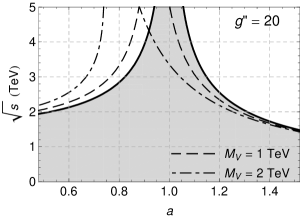
Obviously, the unitarity constraints obtained from Eqs. (21) depend on the mass of the vector resonance as well as on the degree of anomalousness of the scalar resonance coupling $a$. Once $a\neq 1$ the Higgs can no longer guarantee unrestricted unitarity. This problem can be assisted with by invoking additional resonances. The tree-level unitarity constraints as functions of $a$ obtained for various masses of the vector triplet and $g^{\prime\prime}=20$ are shown in Fig. 1. It illustrates the inter-play between the non-SM 125-GeV scalar resonance and the vector triplet in securing the unitarity of the gauge boson scattering amplitudes. With the scalar resonance only, as $a$ departs from one the unitarity limit lowers. Adding the vector resonance triplet tends to improve the unitarity for some $a<1$. On the other hand, when $a>1$, it further lowers the unitarity limit.

Figure 1: The tree-level unitarity constraints from the electroweak gauge-boson scattering as functions of $a$. The shaded area under the solid line depicts the unitarity allowed region for the effective Lagrangian without the vector resonance. The dashed and dot-dashed lines indicate the shift of the region when the $1\;\mathrm{TeV}$ or $2\;\mathrm{TeV}$ vector triplets, respectively, are added. In both cases $g^{\prime\prime}=20$. Zero decay widths of the new resonances are assumed.

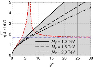
Figure 2: (color online) The tree-level unitarity constraints from the electroweak gauge-boson scattering as functions of $g^{\prime\prime}$. The shaded areas indicate regions where the unitarity holds. The horizontal blue dotted line is the Higgs-less SM unitarity limit of 1.7 TeV. The red dot-dot-dashed line is the unitarity limit when there is the $1\;\mathrm{TeV}$ vector resonance and no Higgs. The black lines indicate the unitarity constraints for the effective Lagrangian with the $a=1$ scalar and the $1\;\mathrm{TeV}$ (solid) or $1.5\;\mathrm{TeV}$ (dashed) or $2\;\mathrm{TeV}$ (dot-dashed) vector resonances. Zero decay widths of the new resonances are assumed. The vertical gray line at $g^{\prime\prime}=25$ indicates the position of the naive perturbativity limit.

Figure 3: (color online) The tree-level unitarity constraints from the electroweak gauge-boson scattering as functions of $g^{\prime\prime}$ for different values of the scalar to gauge boson coupling: $a=1$ (solid), $a=0.7$ (dashed), $a=0.95$ (dot-dashed), and $a=1.1$ (dot-dot-dashed). The $1\;\mathrm{TeV}$ vector resonance and no decay widths are considered.

Figure 2 illustrates the expected behavior: while adding the vector resonance to the Higgs-less SM improves its unitarity limit, it introduces the unitarity problem to the SM with the SM Higgs boson present. Note that in the graph the gray vertical line at $g^{\prime\prime}=25$ indicates the position of the naive perturbativity limit. In the same way the limit will be shown in all following graphs whenever appropriate. In Fig. 3 we show the tree-level unitarity restrictions for the effective Lagrangian when $M_{V}=1\;\mathrm{TeV}$ and $a$ assumes some non-SM values.

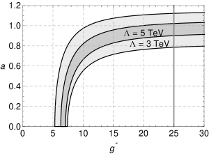
Should the unitarity of the effective Lagrangian hold up to a certain energy the allowed region for the values of $a$ and $g^{\prime\prime}$ can be constructed. The allowed region has a shape of a bent stripe. In particular, the allowed regions for the unitarity constraints of $3$ or $5\;\mathrm{TeV}$ when $M_{V}=1\;\mathrm{TeV}$ are depicted in Fig. 4.

Figure 4: The allowed regions of the $a$ and $g^{\prime\prime}$ parameter space should the tree-level unitarity hold up to $3\;\mathrm{TeV}$ (light gray) and $5\;\mathrm{TeV}$ (dark gray). The $1\;\mathrm{TeV}$ vector resonance and no decay widths are considered.

These findings imply that to secure the tree-level unitarity when $a$ decreases away from its SM value either higher vector resonance mass or lower $g^{\prime\prime}$ have to be invoked. The role of the vector resonance is destructive though if $a$ departs from its SM value in the opposite direction. Of course, in the approximation we use these conclusions are independent of the fermion sector structure of the effective Lagrangian. The observed behavior depends on properties of scalar and vector resonances only. Adding the $SU(2)_{L+R}$ triplet axial-vector resonances or introducing additional constraints on the resonance couplings due to the assumption that the scalar resonance is a pseudo Nambu–Goldstone boson of some sort could alter these conclusions. The investigation of the unitarity question could be refined by considering the gauge boson decay widths and/or additional scattering amplitudes. This would make the unitarity limits sensitive also to the properties of the fermion sector.

4 The low-energy analysis

4.1 Integrating out the vector resonance triplet

If there is the tBESS vector resonance triplet we can learn about its parameters even before its discovery by measuring deviations of the known particle couplings from their SM values. For example, due to the mixing between the vector resonance and the EW gauge bosons the deviations from the SM values would be present in the couplings of the EW gauge bosons to the SM fermions. In this sense, in the case of our effective Lagrangian the most interesting vertices should be those of the top and bottom quarks: $Wtb$, $Zbb$, and $Ztt$.

Unfortunately, the measurements of the $Wtb$ and $Ztt$ vertices has been rather coarse so far TevatronWtb . On the other hand, the couplings of the light fermion vertices including $Zbb$ have been measured at previous colliders, sometimes to a very high precision. We refer to these measurement as the low-energy measurements. While the LHC is capable to refine these measurements, and it has done so already, the existing improvement are not sufficient to compete with the low-energy restrictions on the tBESS parameters. Thus, in our analysis we will focus on the low-energy measurements.

To confront the tBESS free parameters with the low-energy measurements performed at ${\cal O}(10^{2})\;\mathrm{GeV}$, we derive the low-energy (LE) Lagrangian by integrating out the vector resonance triplet the assumed mass of which is ${\cal O}(10^{3})\;\mathrm{GeV}$. It proceeds by taking the limit $M_{triplet}\rightarrow\infty$, while $g^{\prime\prime}$ is finite and fixed, and by substituting the vector resonance equation of motion (EofM) obtained under these conditions. The EofM in the unitarity gauge reads

$$i\frac{g^{\prime\prime}}{2}V_{\mu}^{a}=\frac{1}{2}(igW_{\mu}^{a}+ig^{\prime}B_{\mu}\delta^{a3}),$$ (22)

where $a=1,2,3$. After the EofM is substituted into the unitary gauge ESB Lagrangian (17) the alpha multiplied trace term disappears. We end up with

$${\cal L}_{\mathrm{ESB}}^{\mathrm{LE}} = \frac{1}{2}\partial_{\mu}h\,\partial^{\mu}h-\frac{1}{2}M_{h}^{2}h^{2}-\frac{v^{2}}{4}\mbox{Tr}\left(\mbox{\boldmath$W$}_{\mu}-\mbox{\boldmath$B$}_{\mu}\right)^{2}$$ (23)

$$\times\,\left(1+2a\frac{h}{v}+a^{\prime}\frac{h^{2}}{v^{2}}+\ldots\right).$$

Of course, the EofM has to be substituted in all Lagrangian terms where the vector resonance field occurs. Then, after the gauge boson mass matrix diagonalization and the renormalization of the gauge boson fields the low-energy limit of our effective Lagrangian is obtained.

Since $\alpha\rightarrow\infty$, the number of free parameters in the ESB sector has dropped by one. In the low-energy Lagrangian it is convenient to introduce and use parameters $e$ and $s_{\theta}$ that are related to the strengths of the charged and neutral currents; actually, $e$ is the electric charge and $s_{\theta}$ a counterpart of the Weinberg angle sine. In addition, the parameter $x$ encodes the low-energy residues of the new interaction of the vector resonance triplet. The relations of $e$, $s_{\theta}$, and $x$ to the parameters of the full effective Lagrangian are

$$e=\frac{gg^{\prime}/G}{\sqrt{1+\left(\frac{gg^{\prime}}{Gg^{\prime\prime}/2}\right)^{2}}},\;\;\;s_{\theta}=g^{\prime}/G,\;\;\;x=g/g^{\prime\prime},$$ (24)

where $G=(g^{2}+g^{\prime 2})^{1/2}$. The EW gauge boson masses expressed in terms of $e$, $s_{\theta}$, and $x$ are given by

$$M_{W}^{2}=\frac{g_{\mathrm{LE}}^{2}\,v^{2}}{4},\mbox{\hskip 14.22636pt}M_{Z}^{2}=\frac{G_{\mathrm{LE}}^{2}\,v^{2}}{4},$$ (25)

where $g_{\mathrm{LE}}$ and $G_{\mathrm{LE}}$ are the LE strengths of the charged and neutral currents, respectively. Namely,

$$g_{\mathrm{LE}}^{2}=\frac{1+4s_{\theta}^{2}x^{2}}{1+x^{2}}\,\frac{e^{2}}{s_{\theta}^{2}},\;\;\;G_{\mathrm{LE}}^{2}=\frac{(1+4s_{\theta}^{2}x^{2})^{2}}{c_{\theta}^{2}+x^{2}}\,\frac{e^{2}}{s_{\theta}^{2}},$$ (26)

where $c_{\theta}=(1-s_{\theta}^{2})^{1/2}$.

The EofM also modifies the ${\cal L}_{(t,b)}^{\mathrm{tBESS}}$ term in (6). Thus

$${\cal L}_{\mathrm{ferm}}^{\mathrm{LE}}\equiv{\cal L}_{\mathrm{ferm}}^{\mathrm{SM}}+{\cal L}_{(t,b)}^{\mathrm{LE-tBESS}}+{\cal L}_{\mathrm{ferm}}^{\mathrm{scalar}}.$$ (27)

In the EW gauge boson mass eigenstate basis and after the proper renormalization the relevant parts of the ${\cal L}_{\mathrm{ferm}}^{\mathrm{LE}}$ can be expressed as

$${\cal L}_{\mathrm{ferm}}^{\mathrm{SM}}+{\cal L}_{(t,b)}^{\mathrm{LE-tBESS}} = i\bar{\psi}\!\not{\!\partial}\psi-e\bar{\psi}\!\not{\!\!A}Q\psi$$ (28)

$$-\frac{G_{\mathrm{LE}}}{2}\bar{\psi}\!\not{\!\!Z}(C_{L}P_{L}+C_{R}P_{R})\psi$$

$$-\frac{g_{\mathrm{LE}}}{\sqrt{2}}\bar{\psi}(\!\not{\!\!W}^{+}\tau^{+}+\!\not{\!\!W}^{-}\tau^{-})$$

$$\phantom{-\frac{g_{\mathrm{LE}}}{\sqrt{2}}}\times(D_{L}P_{L}+D_{R}P_{R})\psi,\;\;\;\;\;$$

where $\tau^{\pm}=\tau^{1}\pm i\tau^{2}$, $P_{L,R}=(1\mp\gamma_{5})/2$. For the light fermions (all SM fermions except the top and bottom quarks) $D_{L}=1$, $D_{R}=0$, and

$$C_{L}=2T_{L}^{3}-2\kappa s_{\theta}^{2}Q,\mbox{\hskip 14.22636pt}C_{R}=-2\kappa s_{\theta}^{2}Q,$$ (29)

where

$$\kappa=\frac{1+2x^{2}}{1+4s_{\theta}^{2}x^{2}}.$$ (30)

In the case of the top and bottom quarks,

$$C_{L} = 2(1-\Delta L/2)\,T_{L}^{3}-2\kappa s_{\theta}^{2}Q,$$ (31)

$$C_{R} = 2(P_{f}\,\Delta R/2)\,T_{R}^{3}-2\kappa s_{\theta}^{2}Q,$$ (32)

where $P_{t}=1$, $P_{b}=p^{2}$, and

$$D_{L}=1-\Delta L/2,\mbox{\hskip 14.22636pt}D_{R}=p\;\Delta R/2,$$ (33)

where

$$\Delta L=b_{L}-2\lambda_{L},\mbox{\hskip 14.22636pt}\Delta R=b_{R}+2\lambda_{R}.$$ (34)

Hence, the number of free parameters has been reduced also in the fermion sector of the low-energy Lagrangian. The low-energy observables will depend on the combinations (34) of $b$ and $\lambda$ parameters only. Therefore no limits derived from the low-energy measurements can apply to $b$’s and $\lambda$’s individually.

In order to make numerical predictions the model under consideration must be supplied with an experimental input. The appropriate experimental input in the case of the LE Lagrangian consists of the measured value of the Fermi constant $G_{F}$, the fine structure constant $\alpha$ at the energy scale $M_{Z}$, and the mass $M_{Z}$ of the $Z$ boson. It will prove convenient to replace $G_{F}$ with the sine of the SM Weinberg angle $s_{0}$ using the SM relation

$$\frac{G_{F}}{\sqrt{2}}=\frac{2\pi\,\alpha(M_{Z})}{(2s_{0}c_{0})^{2}M_{Z}^{2}},$$ (35)

where $c_{0}=(1-s_{0}^{2})^{1/2}$. Thus, given the experimental values of $\alpha(M_{Z})$, $M_{Z}$, and $G_{F}$, $s_{0}$ can be considered as a replacement of $G_{F}$ in this list.

The value of $e$ is just a synonym of the measured value of $\alpha$, $e^{2}=4\pi\alpha$. The non-trivial question is how to properly trade $s_{0}$ and $M_{Z}$ for $s_{\theta}$ and $v$. For this we have to write down the LE formula for $G_{F}$,

$$\frac{G_{F}}{\sqrt{2}}=\frac{2\pi\,\alpha(M_{Z})}{(2s_{\theta}c_{\theta})^{2}M_{Z}^{2}}\frac{(1+4s_{\theta}^{2}x^{2})^{2}}{1+(\frac{x}{c_{\theta}})^{2}}.$$ (36)

Then, comparing (36) with (35) we obtain the implicit relation for $s_{\theta}(s_{0},x)$:

$$s_{0}c_{0}=s_{\theta}c_{\theta}\frac{\sqrt{1+(\frac{x}{c_{\theta}})^{2}}}{1+4s_{\theta}^{2}x^{2}}.$$ (37)

To replace the parameter $v$ the LE formula for the $Z$ boson mass,

$$M_{Z}=\frac{ev}{2s_{0}c_{0}},$$ (38)

can be considered.

Regarding the remaining parameters the value of $M_{h}$ is given by the mass of the recently discovered candidate of the Higgs boson. Thus, in the following analysis we will set $M_{h}=125\;\mathrm{GeV}$. Parameters fixed by experiment also include the fermion masses. The existing restrictions on $a,a^{\prime},\ldots$ and $c_{f},c_{f}^{\prime},\ldots$ have been discussed at the end of Section 2. As it was also indicated, there we will perform the best-fit analysis under the simplifying assumption that the scalar resonance couplings are those of the SM. It leaves us with four free parameters that will be used to fit the observables: $x$, $\Delta L$, $\Delta R$, and $p$. In principle, there is also the cut-off scale $\Lambda$ of the LE effective Lagrangian. This is usually related to the mass of the integrated out vector resonance. Our analysis will be performed with the cut-off scale fixed.

4.2 Predictions for the low-energy observables

The deviations of the LE Lagrangian from its SM counterpart modify predictions for the low-energy observables. Thus we can use their measured values to derive the preferences and restrictions on the LE free parameters.

In particular, the experimental limits for the LE-tBESS parameters will be derived by fitting the low-energy (pseudo-)observables, $\epsilon_{1}$, $\epsilon_{2}$, $\epsilon_{3}$, $\Gamma_{b}(Z\rightarrow b\bar{b})$, and BR$(B\rightarrow X_{s}\gamma)$. The epsilons are related to the basic observables EpsilonMethod : the ratio of the electroweak gauge boson masses, $r_{M}\equiv M_{W}/M_{Z}$; the inclusive partial decay width of $Z$ to the charged leptons, $\Gamma_{\ell}(Z\rightarrow\ell\bar{\ell}+\mathrm{photons})$; the forward-backward asymmetry of charged leptons at the $Z$-pole, $A_{\ell}^{FB}(M_{Z})$; and the inclusive partial decay width of $Z$ to bottom quarks, $\Gamma_{b}(Z\rightarrow b\bar{b}+X)$.

The deviations of $r_{M}$, $\Gamma_{\ell}$, and $A_{\ell}^{FB}$ from their predicted SM tree level values including the QED and QCD loop contributions are parameterized by the dynamical corrections $\Delta r_{W}$, $\Delta\rho$, and $\Delta k$ as follows EpsilonMethod :

$$\left(1-r_{M}^{2}\right)r_{M}^{2}=\frac{\pi\alpha(M_{Z})}{\sqrt{2}G_{F}M_{Z}^{2}(1-\Delta r_{W})}$$ (39)

and

$$\Gamma_{\ell} = \frac{G_{F}M_{Z}^{3}}{6\pi\sqrt{2}}(g_{A}^{\ell})^{2}(1+r_{g}^{2})\left(1+\frac{3\alpha}{4\pi}\right),$$ (40)

$$A_{\ell}^{FB} = \frac{3r_{g}^{2}}{(1+r_{g}^{2})^{2}},$$ (41)

where

$$g_{A}^{\ell}=-\frac{1}{2}\left(1+\frac{\Delta\rho}{2}\right),\mbox{\hskip 14.22636pt}r_{g}=\frac{g_{V}^{\ell}}{g_{A}^{\ell}}=1-4(1+\Delta k)s_{0}^{2}.$$ (42)

The three epsilons can be defined as the combinations of the dynamical corrections EpsilonMethod :

$$\epsilon_{1} = \Delta\rho,$$ (43)

$$\epsilon_{2} = c_{0}^{2}\Delta\rho+\frac{s_{0}^{2}}{c_{20}}\Delta r_{W}-2s_{0}^{2}\Delta k,$$ (44)

$$\epsilon_{3} = c_{0}^{2}\Delta\rho+c_{20}\Delta k,$$ (45)

where $s_{0}$ ($c_{0}$) was defined in Eq. (35), and $c_{20}\equiv c_{0}^{2}-s_{0}^{2}$.

The $Zbb$ vertex is naturally tested in the $Z\rightarrow b\bar{b}+X$ decay. The corresponding decay width formula reads EpsilonMethod

$$\Gamma_{b} = \frac{G_{F}M_{Z}^{3}}{6\pi\sqrt{2}}\beta\left[\frac{3-\beta^{2}}{2}(g_{V}^{b})^{2}+\beta^{2}(g_{A}^{b})^{2}\right]\times$$ (46)

$$N_{C}R_{\mathrm{QCD}}\left(1+\frac{\alpha}{12\pi}\right),$$

where $\beta=(1-4m_{b}^{2}/M_{Z}^{2})^{1/2}$, and $R_{\mathrm{QCD}}=1+1.2a-1.1a^{2}-13a^{3}$ is the QCD correction factor, $a=\alpha_{s}(M_{Z})/\pi$.

The precise measurement of $\Gamma_{b}$ can uncover whether the bottom quark anomalous couplings $g_{V,A}^{b}$ differ from the anomalous couplings of other charged SM fermions. Assuming the couplings differ in their $SU(2)_{L}$ parts only, the standard parameterization of the difference is by introducing the parameter $\epsilon_{b}$ EpsilonMethod :

$$g_{A}^{b} = g_{A}^{\ell}(1+\epsilon_{b}),$$ (47)

$$g_{V}^{b} = \left(1+\frac{\Delta\rho}{2}\right)\left[-\frac{1}{2}(1+\epsilon_{b})+\frac{2}{3}(1+\Delta k)s_{0}^{2}\right].$$ (48)

However, our effective Lagrangian admits a more general pattern of the bottom versus light quark anomalous coupling difference than it is assumed in the definition of $\epsilon_{b}$. In our effective Lagrangian the $\epsilon_{b}$ definition assumptions are met when either $p=0$, or $b_{R}=-2\lambda_{R}$. Otherwise, the experimental value of $\Gamma_{b}$ rather then $\epsilon_{b}^{\mathrm{exp}}$ must be related to theoretical prediction in order to derive the low-energy limits on the tBESS free parameters.

The scalar resonance couplings do not contribute to the dynamical corrections at tree level. Thus, the tree-level contributions of the LE Lagrangian to the $\Delta r_{W}$, $\Delta\rho$, and $\Delta k$ as well as to $g_{V,A}^{b}$ are given by the vector resonance sector only. They read

$$\Delta\rho=0,\mbox{\hskip 14.22636pt}\Delta k=\left(\frac{s_{\theta}}{s_{0}}\right)^{2}\kappa(x,s_{\theta})\,-\,1,$$ (49)

$$g_{V}^{b} = \frac{1}{4}(\Delta L-p^{2}\;\Delta R)+\frac{2}{3}\Delta ks_{0}^{2},$$ (50)

$$g_{A}^{b} = \frac{1}{4}(\Delta L+p^{2}\;\Delta R).$$ (51)

The tree-level contribution to $\Delta r_{W}$ is obtained from the LE expression for the ratio $r_{M}=M_{W}/M_{Z}$. It reads

$$r_{M}^{2}=\frac{c_{\theta}^{2}+x^{2}}{(1+4s_{\theta}^{2}x^{2})(1+x^{2})}.$$ (52)

Then

$$\Delta r_{W}=1-\left(\frac{1+x^{2}}{1+2x^{2}}\right)^{2}.$$ (53)

Now, the tree-level contributions to $\epsilon_{i}$’s can be obtained from the dynamical corrections using Eqs. (43) through (45):

$$\epsilon_{1} = 0,$$

$$\epsilon_{2} = \frac{s_{0}^{2}}{c_{20}}\frac{x^{2}(2+3x^{2})}{(1+2x^{2})^{2}}-2s_{0}^{2}\,\Delta k(x),$$

$$\epsilon_{3} = c_{20}\,\Delta k(x),$$

where $\Delta k(x)$ is given in (49). The leading terms of the epsilon expansions in powers of $x$ at $x=0$ read

$$\epsilon_{2} = -2.71\,x^{4}+2.96\,x^{6}+\ldots,$$ (54)

$$\epsilon_{3} = x^{2}+0.66\,x^{4}+2.56\,x^{6}+\ldots.$$ (55)

There is no reason to expect that the LE anomalies at the tree level overwhelm the 1-loop contributions of the LE Lagrangian to the epsilons. Thus, both contributions should be considered when predicting the epsilon observables

$$\epsilon_{i}=\epsilon_{i}^{\mathrm{LE(0)}}+\epsilon_{i}^{\mathrm{LE(1)}},\mbox{\hskip 14.22636pt}i=1,2,3,b,$$ (56)

where $\mathrm{LE(0)}$ and $\mathrm{LE(1)}$ denotes the tree-level and 1-loop contributions of the LE Lagrangian, respectively.

Since we study an effective non-renormalizable Lagrangian, it is not that obvious how to properly deal with the higher order calculations Malkawi . One does not know the underlying theory therefore there is no way to establish a correct scheme for the effective Lagrangian Georgi . While the divergent piece in loop calculations can be associated with a physical cut-off $\Lambda$ up to which the effective Lagrangian is valid PecceiZhang , for the finite piece there is no completely satisfactory approach available BurgessLondon .

We approximate $\epsilon_{i}^{\mathrm{LE(1)}}$ by the sum of the SM weak loop corrections $\epsilon_{i}^{\mathrm{SM(1)}}$ representing the loop contributions from the scalar resonance and the vector resonance related loop contributions $\epsilon_{i}^{\mathrm{vec}(1)}$:

$$\epsilon_{i}^{\mathrm{LE}(1)}\approx\epsilon_{i}^{\mathrm{SM(1)}}+\epsilon_{i}^{\mathrm{vec}(1)}.$$ (57)

The $\epsilon_{i}^{\mathrm{SM(1)}}$ contributions are given by the following relations newBESS :

$$\epsilon_{1}^{\mathrm{SM(1)}} = \left(+5.60-0.86\ln\frac{M_{h}}{M_{Z}}\right)\times 10^{-3},$$ (58)

$$\epsilon_{2}^{\mathrm{SM(1)}} = \left(-7.09+0.16\ln\frac{M_{h}}{M_{Z}}\right)\times 10^{-3},$$ (59)

$$\epsilon_{3}^{\mathrm{SM(1)}} = \left(+5.25+0.54\ln\frac{M_{h}}{M_{Z}}\right)\times 10^{-3},$$ (60)

$$\epsilon_{b}^{\mathrm{SM(1)}} = -6.43\times 10^{-3}.$$ (61)

For $M_{h}=125\;\mathrm{GeV}$ and $M_{Z}=91.1876\;\mathrm{GeV}$ the following SM contributions are obtained: $\epsilon_{1}^{\mathrm{SM(1)}}=5.33\times 10^{-3}$, $\epsilon_{2}^{\mathrm{SM(1)}}=-7.04\times 10^{-3}$, and $\epsilon_{3}^{\mathrm{SM(1)}}=5.42\times 10^{-3}$.

The 1-loop SM contributions to $g_{V}^{b}$ and $g_{A}^{b}$ can be obtained by subtracting the SM tree-level couplings from the SM tree plus 1-loop couplings:

$$(g_{V,A}^{b})^{\mathrm{SM(1)}}=(g_{V,A}^{b})^{\mathrm{SM(0+1)}}-(g_{V,A}^{b})^{\mathrm{SM(0)}},$$ (62)

where $(g_{V,A}^{b})^{\mathrm{SM(0+1)}}$ are given by Eqs. (47) and (48) if $\Delta\rho=(\Delta\rho)^{\mathrm{SM(1)}}$, $\Delta k=(\Delta k)^{\mathrm{SM(1)}}$, and $\epsilon_{b}=\epsilon_{b}^{\mathrm{SM(1)}}$ are applied. Of course, $(g_{V}^{b})^{\mathrm{SM(0)}}=-1/2+2s_{0}^{2}/3$ and $(g_{A}^{b})^{\mathrm{SM(0)}}=-1/2$.

The $\epsilon_{i}^{\mathrm{vec}(1)}$ contributions can be calculated using the results of LariosKappaAnalysis . The paper provides expressions for new physics loop contributions to the epsilon parameters in terms of generic anomalous couplings of the non-linear electroweak chiral Lagrangian. Up to the order of $m_{t}^{2}\ln\Lambda^{2}$ the anomalous loop contributions read

$$\epsilon_{1}^{\mathrm{NP(1)}} = \frac{3m_{t}^{2}G_{F}}{2\sqrt{2}\pi^{2}}\ln\frac{\Lambda^{2}}{m_{t}^{2}}\left[\kappa_{L}^{Wtb}\left(1+{\kappa_{L}^{Wtb}}\right)\right.$$ (63)

$$+\left.\left(\kappa_{R}^{Ztt}-\kappa_{L}^{Ztt}\right)\left(1-\kappa_{R}^{Ztt}+\kappa_{L}^{Ztt}\right)\right],$$

$$\epsilon_{2}^{\mathrm{NP(1)}} = \epsilon_{3}^{\mathrm{NP(1)}}\;=\;0\,,$$ (64)

where $\Lambda$ is the cut-off scale of the effective Lagrangian under consideration. In the cases when the $\mathrm{NP(1)}$ contributions depend on $\kappa^{Zbb}$ the dependence is suppressed by $m_{b}\ll m_{t}$.

In our case, when $\Lambda=1$ TeV and using the numerical values of A, the leading terms of the $x^{2}$ series of $\epsilon_{1}^{\mathrm{vec}(1)}$ read

$$\frac{\epsilon_{1}^{\mathrm{vec}(1)}}{10^{-2}} = \phantom{-}6.57\,\Delta R-2.82\,(2-3\,\Delta L)\,x^{2}+\ldots,$$ (65)

where we have also neglected non-linear terms in $\Delta L$, $\Delta R$. The $\epsilon_{1}^{\mathrm{vec}(1)}$ series for $\Lambda=2$ TeV is obtained when (65) is multiplied by the numerical factor of $1.39$.

In our analysis, we have not calculated $(g_{V,A}^{b})^{\mathrm{vec}(1)}$. The fit is based on the $\mathrm{LE(0)}$ and $\mathrm{SM(1)}$ contributions to $g_{V,A}^{b}$ only. Thus obtained $g_{V,A}^{b}$ are, in turn, substituted to Eq. (46). We justified this simplifying approximation by comparing the single-observable fits based on $\epsilon_{b}^{\mathrm{LE(0)}+\mathrm{SM(1)}+\mathrm{vec}(1)}$ with the fits based on $(g_{V,A}^{b})^{\mathrm{LE(0)}+\mathrm{SM(1)}}$ when $p=0$, see tBESS . Figure of tBESS illustrates that the absence of the $\mathrm{vec}(1)$ contribution in the latter fits introduces only relatively small shifts in the obtained confidence level contours.

The $B\rightarrow X_{s}\gamma$ decay puts limits on the anomalous $W^{\pm}t_{L}b_{L}$ and $W^{\pm}t_{R}b_{R}$ vertices Malkawi ; LariosKappaAnalysis . In the SM it proceeds through the flavor changing neutral current loop process $b\rightarrow s\gamma$ dominated by the top quark exchange diagram. The $B\rightarrow X_{s}\gamma$ branching fraction can be sensitive to physics beyond the SM via new particles entering the penguin loop. When expressed in terms of the real anomalous $Wtb$ couplings, $\kappa_{L}^{Wtb}$ and $\kappa_{R}^{Wtb}$, it can be approximated by the following formula LariosKappaAnalysis :

$$\mbox{BR}(B\rightarrow X_{s}\gamma)\times 10^{4} = 3.07+280\,\kappa_{R}^{Wtb}+2\,\kappa_{L}^{Wtb}$$ (66)

$$+5520\,(\kappa_{R}^{Wtb})^{2}+0.3\,(\kappa_{L}^{Wtb})^{2}$$

$$+79\,\kappa_{L}^{Wtb}\kappa_{R}^{Wtb}.$$

The expressions for the LE anomalous couplings that are needed in the formulas (63) and (66) are given in B.

4.3 Fits and limits

Using the formulas for the LE predictions we have performed a multi-parameter $\chi^{2}$ fit of the observables in order to obtain the most preferred values and confidence level intervals for the LE-tBESS parameters. The set of fitted observables consists of $\epsilon_{1}$,$\epsilon_{2}$,$\epsilon_{3}$,$\Gamma_{b}$, and $\mbox{BR}(B\rightarrow X_{s}\gamma)$. The experimental values of the observables used in this analysis are shown in A.

By fitting the five observables mentioned above with the four free parameters — $x$, $\Delta L$, $\Delta R$, and $p$ — we found the best values

$$g^{\prime\prime}(x)=29,\quad\Delta L=-0.004,\quad p\;\Delta R=0.003,$$ (67)

with $\chi^{2}_{min}=2.40$. Since $\mathrm{d.o.f.}=5-4=1$, the obtained value of $\chi^{2}_{min}$ corresponds to the backing of $12\%$. Within the rounding errors these values hold for the cut-off scale between $0.3\;\mathrm{TeV}\leq\Lambda\leq 10^{3}\;\mathrm{TeV}$, at least. The best values of $p$ and $\Delta R$ depend on $\Lambda$, separately; in particular,

$$\Lambda=1\;\mathrm{TeV}: \quad\Delta R=0.016\quad p=0.209$$ (68)

$$\Lambda=2\;\mathrm{TeV}: \quad\Delta R=0.011\quad p=0.289$$ (69)

Note that the best-fit value of $g^{\prime\prime}$ falls into the regions allowed by the unitarity. Further, the preferred value of $p$ supports the idea about stronger right-top than right-bottom coupling of the vector resonance. The higher value of $g^{\prime\prime}$ is certainly preferable considering the assumed strong nature of underlying fundamental theory. On the other hand, the best value is somewhat above the naive perturbativity limit of 25. Of course, the results of our analysis are certainly not reliable above perturbativity limit. Nevertheless, following the reasons discussed in Section 2 we will show results for $g^{\prime\prime}$ up to 30.

The observables $\epsilon_{1}$ and $\Gamma(B\rightarrow X_{s}\gamma)$ are essential in the explanation the observed behavior of the preferred values of $p$ and $\Delta R$. The parameters $p$ and $\Delta R$ enter three of the considered observables only. Namely, these are $\epsilon_{1}$, $\Gamma_{b}(Z\rightarrow b\bar{b})$, and $\Gamma(B\rightarrow X_{s}\gamma)$. While $\epsilon_{1}$ depends on $\Delta R$ solely, $\Gamma(B\rightarrow X_{s}\gamma)$ depends on the product $p\,\Delta R$ and $\Gamma_{b}$ depends on $p^{2}\Delta R$. The sensitivity to $\Lambda$ enters through $\epsilon_{1}$ only.

Since the free parameter space is four-dimensional, it is impossible to graphically depict the CL regions around the best-fitting point. Nevertheless, we can quote the marginalized intervals — the one-dimensional projections of the confidence region — for each parameter. In our case, the marginalized intervals of the $95\%$ CL region read

$$\begin{array}[]{ccccc}12&\leq&g^{\prime\prime}&&\\ -0.013&\leq&\Delta L&\leq&0.006\\ -0.006&\leq&\Delta R&\leq&0.056\end{array}$$ (70)

when $\Lambda=1\;\mathrm{TeV}$ and $p\geq 0$ is assumed. The value of $p$ is restricted only very mildly by the considered data. The whole physically motivated interval $0\leq p\leq 1$ belongs to the marginalized interval of the $95\%$ CL region. The change of the cut-off scale to $\Lambda=2\;\mathrm{TeV}$ alters only the marginalized interval for $\Delta R$,

$$\begin{array}[]{ccccc}-0.005&\leq&\Delta R&\leq&0.041\end{array}$$ (71)

and leaves all other conclusions basically intact. Let us note that the limit $g^{\prime\prime}\geq 12$ is implied by the restriction $0\leq x\leq 0.056$.

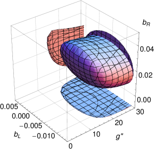
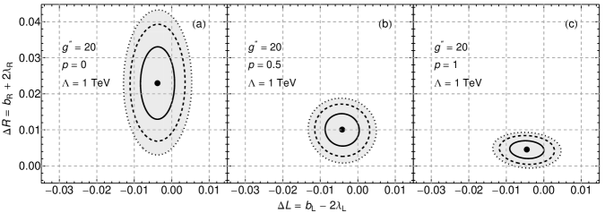
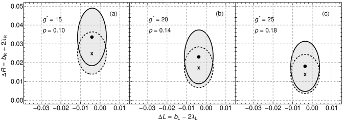
Since the value of $p$ can be motivated by theory, e.g. by the models of the partial compositeness, it might be useful to depict a three-dimensional cut of the four-dimensional $95\%$ CL region for some fixed value of $p$. We choose the best value of $p=0.209$ for $\Lambda=1\;\mathrm{TeV}$, see Eq. (68). The obtained three-dimensional allowed region of the parameters $x$, $\Delta L$, and $\Delta R$ is shown in Fig. 5.

Figure 5: (color online) The $p=0.209$ cut of the 95% CL allowed region of the parameters $\{g^{\prime\prime},\Delta L,\Delta R,p\}$ when $\Lambda=1\;\mathrm{TeV}$. The 2D projections of the allowed region to $(g^{\prime\prime},\Delta L)$, $(g^{\prime\prime},\Delta R)$, and $(\Delta L,\Delta R)$ planes are also shown.

Only the $g^{\prime\prime}\leq 30$ part of the region is shown in the graph. The region is not restricted in $g^{\prime\prime}$ from above.

It is certainly interesting to see how the best-fitting values of the free parameters would change if some of the parameters are fixed, presumably by theoretical assumptions. Actually, even if there were no theoretical presumption for fixing the value of a particular parameter by studying plots where some of the free parameters are fixed ahead better understanding of behavior of the full four-parameter fit can be achieved. One just has to be careful when interpreting such graphs; e.g., in assigning a correct backing to a set of parameter values. Having said that, in Fig. 6 we show the best-fit values of $x$ ($p$) when the values of $p$ ($x$) have been fixed beforehand. Of course, $\Delta L$ and $\Delta R$ are the remaining free parameters in the fit. Thus, $\mathrm{d.o.f.}=5-3=2$ in this case.

     

Figure 6: (color online) The graphs of the best-fit values of $p$ (red solid line) and $g^{\prime\prime}$ (blue dashed line) as functions of beforehand fixed values of, respectively, $g^{\prime\prime}$ and $p$. The remaining fitting parameters are $\Delta L$ and $\Delta R$. The gray dotted contours intersect the curves at points with $1\%$, $5\%$, $10\%$, $15\%$, $20\%$, and $25\%$ backings ($\mathrm{d.o.f.}=2$). The intersection of the dashed blue and solid red curves possesses a $30\%$ backing. The left and right panels correspond to $\Lambda=1\;\mathrm{TeV}$ and $\Lambda=2\;\mathrm{TeV}$, respectively.

The contour dashed lines in Fig. 6 connect the points with the same backings in the fits by free parameters $\Delta L$ and $\Delta R$ if both — $x$ and $p$ — are fixed beforehand. In this case, $\mathrm{d.o.f.}=5-2=3$. The $\chi^{2}_{\mathrm{min}}$ values for various combinations of fixed $g^{\prime\prime}$ and $p$ are shown in Fig. 7.

Figure 7: (color online) $\chi^{2}_{min}$ of the fit by $\Delta L$ and $\Delta R$ as a function of the fixed parameters $g^{\prime\prime}$ and $p$ for $\Lambda=1\;\mathrm{TeV}$. The labels on the r.h.s. axis indicate the backings for $\mathrm{d.o.f.}=3$.

We can see that the best backing for the fits is getting less pronounced as $g^{\prime\prime}$ approaches $30$ from below. More specifically, while backings of the fits with different $p$’s can differ by several orders of magnitude when $g^{\prime\prime}\stackrel{{\scriptstyle<}}{{\sim}}20$, the backing for $g^{\prime\prime}=30$ changes between $10$ and $50\%$ as $p$ crawls along the $\langle 0;1\rangle$ interval.

The best-fit values of $\Delta L$ and $\Delta R$ for the given $g^{\prime\prime}$ and $p$ can be read off of the graphs in Fig. 8. Besides, the contours connecting the $(g^{\prime\prime},p)$ points with the same backings are shown there, too.

Figure 8: (color online) The contours (black solid lines) connecting the $(g^{\prime\prime},p)$ points with the same backings in the fit by free parameters $\Delta L$ and $\Delta R$. The backing values shown on the contours correspond to $\mathrm{d.o.f.}=3$. The graphs also contain the grid from which the best-fit values of $\Delta L$ (red dot-dashed) and $\Delta R$ (blue dashed) for each given pair of fixed values $(g^{\prime\prime},p)$ can be read off. The numbers attached to the grid lines are $10^{3}$ times the actual values represented by the lines. The left and right panels display the $\Lambda=1\;\mathrm{TeV}$ and $\Lambda=2\;\mathrm{TeV}$ cases, respectively.

Table 1 lists explicitly some of the best-fit values of $\Delta L$ and $\Delta R$ corresponding to the assortment of fixed $g^{\prime\prime}$ and $p$ values.

Table 1: The best-fit values of $\Delta L$ and $\Delta R$ found in the fits for various fixed values of $g^{\prime\prime}$ and $p$ when $\Lambda=1$ TeV. The backing shown corresponds to $\mathrm{d.o.f}=5-2=3$.

fixed		best fits
$g^{\prime\prime}$	$p$	$\Delta L$	$\Delta R$	$\chi^{2}_{min}$	Backing (%)
15	0.10	-0.0042	0.0336	4.94	17.60000
20	0	-0.0038	0.0229	6.18	10.30000
20	0.14	-0.0038	0.0231	2.81	42.20000
20	0.5	-0.0042	0.0101	7.65	5.40000
20	1	-0.0045	0.0046	11.77	1.10000
25	0.18	-0.0037	0.0181	2.44	48.60000
30	0.2	-0.0036	0.0157	2.42	49.10000

Eventually, in Fig. 9 we show the allowed CL regions for the fits around some selected combinations of $g^{\prime\prime}$ and $p$ parameters considered also in Table 1. In particular, we display contours for $g^{\prime\prime}=20$ and three different values of $p$. Note that the backings for different values of $p\in\langle 0;1\rangle$ when $g^{\prime\prime}\approx 20$ do not change significantly (see Figs. 7 and 8). The backings for $g^{\prime\prime}=20$, $\Lambda=1\;\mathrm{TeV}$, and $p=0$, $0.5$, and $1$ are about $10\%$, $5\%$, and $1\%$, respectively. Since $\Delta L$ is predominantly related to a different observable ($\Gamma_{b}$) than $\Delta R$ and $p$ ($\epsilon_{1}$, $\Gamma(B\rightarrow X_{s}\gamma)$), it is not unexpected that the changes in $p$ affect $\Delta R$ only. In all three displayed cases the $95\%$ C.L. allowed interval for $\Delta L$ reads $(-0.012,0.003)$. The $95\%$ C.L. allowed interval for $\Delta R$ is $(0.007,0.039)$ when $p=0$. It shrinks to $\Delta R\in(0.000,0.008)$ when $p=1$.

Figure 9: The 90% C.L. (solid line), 95% C.L. (dashed line), and 99% C.L. (dotted line) allowed regions in the $(\Delta L,\Delta R)$ parameter space. The regions are derived from the two-parameter fit by $\Delta L$ and $\Delta R$ for $g^{\prime\prime}=20$, $\Lambda=1$ TeV, and (a) $p=0$, (b) $0.5$, and (c) $1$. The best-fit values of $\Delta L$ and $\Delta R$ are indicated by the dots.

The effect of altering $g^{\prime\prime}$ and/or $\Lambda$ is illustrated in Fig. 10. There, the 95% C.L. allowed regions in the $(\Delta L,\Delta R)$ parameter space when $p$ assumes the values $0.10$, $0.14$, and $0.18$ are shown. These are the $p$ values with the highest backings for $g^{\prime\prime}=15$, $20$, and $25$, respectively. The corresponding best-fit $\Delta L$ and $\Delta R$, $\chi^{2}_{\mathrm{min}}$’s and backings are shown in Table 1. The allowed regions are shown for the cut-off scales $\Lambda=1\;\mathrm{TeV}$ and $\Lambda=2\;\mathrm{TeV}$. As far as the allowed regions are concerned, $\Delta L$ falls within $(-0.012,0.004)$, independently of the other parameter values. For $\Lambda=1\;\mathrm{TeV}$, the $\Delta R$ limits read $(0.018,0.049)$ when $g^{\prime\prime}=15$, $(0.009,0.037)$ when $g^{\prime\prime}=20$, and $(0.005,0.032)$ when $g^{\prime\prime}=25$. For $\Lambda=2\;\mathrm{TeV}$, the $\Delta R$ limits read $(0.014,0.036)$ when $g^{\prime\prime}=15$, $(0.007,0.028)$ when $g^{\prime\prime}=20$, and $(0.004,0.024)$ when $g^{\prime\prime}=25$.

Figure 10: The 95% C.L. allowed regions in the $(\Delta L,\Delta R)$ parameter space derived from the same fit as in Fig. 9 except for the values of the fixed parameters. The solid contours correspond to $\Lambda=1\;\mathrm{TeV}$, the dashed ones to $\Lambda=2\;\mathrm{TeV}$. The values of the fixed parameters $g^{\prime\prime}$ and $p$ are, respectively, (a) $15$ and $0.10$, (b) $20$ and $0.14$, and (c) $25$ and $0.18$. The best-fit values of $\Delta L$ and $\Delta R$ are indicated by the dot and cross for $\Lambda=1\;\mathrm{TeV}$ and $\Lambda=2\;\mathrm{TeV}$, respectively.

Having the data preferred values of the LE Lagrangian parameters we can evaluate the strengths of the direct interaction vertices of the vector resonance triplet with the top and bottom quarks. For the sake, we will recall the vertices of the vector resonance triplet with the top and bottom quarks that have been derived in tBESS . In the gauge boson flavor basis they read

$$c^{Vtt}_{L}=\sqrt{2}\,c^{Vtb}_{L}=-c^{Vbb}_{L} = -\phantom{p^{2}}\,b_{L}\,g^{\prime\prime}/4$$

$$c^{Vtt}_{R}\phantom{=\sqrt{2}\,c^{Vtb}_{L}=-c^{Vbb}_{L}} = -\phantom{p^{2}}\,b_{R}\,g^{\prime\prime}/4$$

$$\phantom{c^{Vtt}_{R}=}\sqrt{2}\,c^{Vtb}_{R}\phantom{=-c^{Vbb}_{L}} = -p\phantom{{}^{2}}\,b_{R}\,g^{\prime\prime}/4$$

$$\phantom{c^{Vtt}_{R}=\sqrt{2}\,c^{Vtb}_{R}=}-c^{Vbb}_{R} = -p^{2}\,b_{L}\,g^{\prime\prime}/4$$

Of course, in the mass eigenstate basis these terms must be supplemented with the contributions from the gauge boson mixing. Recall that the mixing-induced interactions are proportional to $1/g^{\prime\prime}$ and thus represent minor corrections. We choose to evaluate the direct couplings at the best-fit values of the free parameters $\Delta L$, $\Delta R$, and $p$ when $g^{\prime\prime}=20$ and $\Lambda=1\;\mathrm{TeV}$ ($2\;\mathrm{TeV}$), i.e. $-0.0038$ ($-0.0039$), $0.0231$ ($0.0166$), and $0.14$ ($0.20$), respectively. Since the existing data restrict only the combinations of $b_{L,R}$ and $\lambda_{L,R}$ we will assume that $\lambda_{L,R}=0$. The obtained coupling values are shown in Table 2. If $\lambda$’s are allowed to vary we expect that the best-fit couplings can double or reduce by half without being accused of fine-tuning conspiracy between $b_{L,R}$’s and $\lambda_{L,R}$’s.

Table 2: The couplings of the vector triplet to top/bottom quark vertices when $\lambda_{L,R}=0$ corresponding to the best-fit values of $\Delta L$, $\Delta R$, and $p$ when $g^{\prime\prime}=20$.

$\Lambda$	$g^{\prime\prime}b_{L}/4$	$g^{\prime\prime}b_{R}/4$	$pg^{\prime\prime}b_{R}/4$	$p^{2}g^{\prime\prime}b_{R}/4$
1 TeV	-0.0190	0.1155	0.0162	0.0023
2 TeV	-0.0195	0.0830	0.0166	0.0033

In some models of partial fermion compositeness the masses of the SM fermions are related to the product of compositeness $\varepsilon_{L,R}^{f}$ of the left and right chirality CHsketch ; Sundrum ; PomarolSerra . The same compositeness factors govern the strength of the couplings of the new strong resonances to the fermions. Naively, we can relate these considerations with the tBESS parameters as follows:

$$\varepsilon_{L}^{t,b}\propto b_{L},\mbox{\hskip 14.22636pt}\varepsilon_{R}^{t}\propto b_{R},\mbox{\hskip 14.22636pt}\varepsilon_{R}^{b}\propto pb_{R}.$$ (72)

Then

$$\frac{m_{b}}{m_{t}}=\frac{\varepsilon_{L}^{b}\varepsilon_{R}^{b}}{\varepsilon_{L}^{t}\varepsilon_{R}^{t}}=p.$$ (73)

This example illustrates how the tBESS parameters can be related to and fixed by predictions of specific models. In this particular case, the predicted value of $p$ is about $0.03$. This is quite away from the best fit $p\stackrel{{\scriptstyle>}}{{\sim}}0.2$ found in our analysis. However, the best value of $p$ is not restricted very tightly by the analyzed data; $p=0.03$ is still within the $95\%$ CL region of the best fit by the four parameters.

If we fix $p=0.03$ as predicted by some models with the partial fermion compositeness then the best values of the remaining free parameters are $g^{\prime\prime}=24$, $\Delta L=-0.004$, and $\Delta R=0.020$ when $\Lambda=1\;\mathrm{TeV}$. Since $\chi^{2}=4.79$ the backing of this fit is about $9\%$. If we assume $\Lambda=2\;\mathrm{TeV}$ then the numbers change as follows: $g^{\prime\prime}=25$, $\Delta L=-0.004$, $\Delta R=0.014$, and $\chi^{2}=5.06$, therefore the backing is about $8\%$.

5 Conclusions

We have formulated and studied the effective Lagrangian for description of phenomenology of new scalar and vector resonances which might result from new strong physics beyond the SM. Following the often used and studied approach the ESB sector of the effective Lagrangian has been based on the $SU(2)_{L}\times SU(2)_{R}\rightarrow SU(2)_{L+R}$ non-linear sigma model while the scalar resonance has been introduced as the $SU(2)_{L+R}$ singlet and identified with the newly discovered 125-GeV boson. The vector resonance has been built in as the $SU(2)_{L+R}$ triplet employing the hidden local symmetry approach. Throughout the paper we have assumed the vector resonance mass at the bottom of the TeV scale. No other non-SM fields have been considered in our effective Lagrangian.

Within this general framework we have invoked a special pattern of interactions between the vector resonances and the SM fermions. Beside the gauge boson mixing induced interactions the symmetry of the Lagrangian admits the direct interactions of the vector triplet to the SM fermions. Motivated by experimental as well as theoretical considerations we have opted for the pattern where the vector resonance couples directly to the third quark generation only. The couplings are chiral-dependent and the interaction of the right top quark can differ from that of the right bottom quark. Similar interaction patterns can be found in various recent extensions of the SM including extra-dimensional and composite scenarios.

We have analyzed the tree-level unitarity of the gauge boson scattering amplitudes to estimate the applicability range of our effective Lagrangian. In particular, we have been investigating how the presence of both, scalar and vector, resonances affects the unitarity restrictions. Adding the vector resonance triplet tends to improve the unitarity when the coupling of the scalar to the gauge fields, $a$, is lower than its SM value, $a=1$. For $a>1$ the presence of the vector triplet further lowers the unitarity limit. In general, the unitarity holds in the regions of $a$ and $g^{\prime\prime}$ that are also preferred by experiment. Recall that $g^{\prime\prime}$ is the vector resonance triplet gauge coupling.

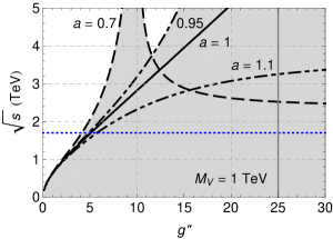
We have also analyzed the experimental limits on the free parameters of the vector resonance triplet under the assumption of the SM couplings for the scalar resonance. This was a simplifying assumption that allowed us to focus on the vector resonance parameters before any more complex and sophisticated investigation would be undertaken. The assumption is in agreement with the current experimental findings about the new 125-GeV boson. The results found in our analysis could also be considered as an approximation of the situation when the scalar resonance parameters slightly differ from their SM values.

Since LHC measurements vertices are not restrictive enough we have calculated the preferred values and CL intervals for the vector resonance couplings from the low-energy observables only. Namely, we have fitted five observables, $\epsilon_{1}$, $\epsilon_{2}$, $\epsilon_{3}$, $\Gamma_{b}$, and $\mathrm{BR}(B\rightarrow X_{s}\gamma)$, parameterized by four free parameters, $g^{\prime\prime}$, $\Delta L=b_{L}-2\lambda_{L}$, $\Delta R=b_{R}-2\lambda_{R}$, and $p$. When the cut-off scale $\Lambda=1\;\mathrm{TeV}$ the best-fit values read $g^{\prime\prime}=29$, $\Delta L=-0.004$, $\Delta R=0.016$, and $p=0.209$ with $\chi^{2}/\mathrm{d.o.f.}=2.40/1$ which corresponds to the $12\%$ backing. The marginalized intervals of the $95\%$ CL region for individual parameters read $g^{\prime\prime}\geq 12$, $-0.013\leq\Delta L\leq 0.006$, $-0.006\leq\Delta R\leq 0.056$. The marginalized interval for $p$ includes whole physically motivated interval $0\leq p\leq 1$. Note that while the best-fit value of $g^{\prime\prime}$ is somewhat above the naive perturbativity limit the perturbativity region overlaps with the found restriction on $g^{\prime\prime}$. Recall that the direct vector resonance coupling to the left top-bottom quark doublet is proportional to $b_{L}g^{\prime\prime}$ and the direct coupling to the right top quark is proportional to $b_{R}g^{\prime\prime}$. With respect to the latter, the couplings of the right bottom quark to the charged and neutral vector resonances are diminished by $p$ and $p^{2}$, respectively. The parameters $\lambda_{L,R}$ parameterize the non-SM couplings of the EW gauge bosons allowed by the symmetry. With the low-energy measurements only one cannot obtain limits on the $b$ and $\lambda$ parameters separately.

The best-fit value of $p$ found in our analysis seems to support the assumption of some models of partial fermion compositeness that the new strong physics resonances couple stronger to the right top quark than to the right bottom quark. Unfortunately, when $g^{\prime\prime}$ is set close to its most preferred value then any $p$ within the $\langle 0;1\rangle$ interval has comparable experimental support. Therefore, while the low-energy data seems to point in the right direction any strong statements about the preferred value of $p$ would be premature at this point. Unless the vector resonance is discovered directly, further progress in the LHC measurements of the $Ztt$ and $Wtb$ vertices is needed to improve limits on this and other parameters of the studied effective Lagrangian.

Appendix A Experimental values

In our analyses we have used the experimental values of the epsilon pseudo-observables obtained from a fit to all LEP-I and SLD measurements including the combined preliminary measurement of the $W$-boson mass EpsilonData :

$$\epsilon_{1}^{\mathrm{exp}} = (+5.4\phantom{4}\pm 1.0)\times 10^{-3},$$ (74)

$$\epsilon_{2}^{\mathrm{exp}} = (-8.9\phantom{4}\pm 1.2)\times 10^{-3},$$ (75)

$$\epsilon_{3}^{\mathrm{exp}} = (+5.34\pm 0.94)\times 10^{-3},$$ (76)

$$\epsilon_{b}^{\mathrm{exp}} = (-5.0\phantom{4}\pm 1.6)\times 10^{-3},$$ (77)

with the correlation matrix

$$\rho^{\epsilon}=\left(\begin{array}[]{cccc}1.00&\phantom{-}0.60&\phantom{-}0.86&\phantom{-}0.00\\ 0.60&\phantom{-}1.00&\phantom{-}0.40&-0.01\\ 0.86&\phantom{-}0.40&\phantom{-}1.00&\phantom{-}0.02\\ 0.00&-0.01&\phantom{-}0.02&\phantom{-}1.00\\ \end{array}\right).$$ (82)

The value of the $Z\rightarrow b\bar{b}$ decay width

$$\Gamma_{b}^{\mathrm{exp}}=(0.3773\pm 0.0013)\ \mathrm{GeV}$$ (83)

has been obtained from the experimental values PDG2010 :

$$\mbox{BR}(Z\rightarrow b\bar{b})^{\mathrm{exp}} = (0.1512\pm 0.0005),$$ (84)

$$\Gamma_{tot}(Z)^{\mathrm{exp}}\;\;\;\;\; = (2.4952\pm 0.0023)~{}\mbox{GeV}.$$ (85)

The correlations between $\Gamma_{b}$ and $\epsilon_{1,2,3}$ have been neglected.

For the branching fraction of $B\rightarrow X_{s}\gamma$ we have used the world average btosgData (CLEO, Belle, BaBar):

$$\mbox{BR}(B\rightarrow X_{s}\gamma)^{\mathrm{exp}}=(3.55\pm 0.26)\times 10^{-4}.$$ (86)

We have considered no correlations between $\mbox{BR}(B\rightarrow X_{s}\gamma)$ and any of the observables $\epsilon_{1},\epsilon_{2},\epsilon_{3},\Gamma_{b}$.

Below we will complete the list of numerical values that have been used in the calculations of this paper:

$$\alpha(0) = 1/137.036,$$ (87)

$$\alpha(M_{Z}^{2}) = 1/128.91,$$ (88)

$$\alpha_{s}(M_{Z}^{2}) = 0.1184,$$ (89)

$$G_{F} = 1.166364\times 10^{-5}\ \mathrm{GeV^{-2}},$$ (90)

$$m_{b} = 4.67\ \mathrm{GeV},$$ (91)

$$m_{t} = 172.7\ \mathrm{GeV},$$ (92)

$$M_{Z} = 91.1876\ \mathrm{GeV},$$ (93)

$$M_{h} = 125\ \mathrm{GeV}.$$ (94)

Then, using Eq. (35) the numerical value of $s_{0}^{2}$ is

$$s_{0}^{2}=0.2311.$$ (95)

Appendix B Some anomalous couplings

Here we show the anomalous couplings found in the formulas (63) and (66) for the loop contributions $\epsilon_{1}^{\mathrm{vec}(1)}$ and $\mathrm{BR}(B\rightarrow X_{s}\gamma)$, respectively. They read:

$$\kappa_{L}^{Wtb} = h(x;s_{0})\left(1-\frac{\Delta L}{2}\right)-1,$$ (96)

$$\kappa_{R}^{Wtb} = h(x;s_{0})\;\frac{p\;\Delta R}{2},$$ (97)

$$\kappa_{L}^{Ztt} = -\frac{1}{2}\Delta L-\frac{4}{3}s_{0}^{2}\;\Delta k(x;s_{0}),$$ (98)

$$\kappa_{R}^{Ztt} = +\frac{1}{2}\Delta R-\frac{4}{3}s_{0}^{2}\;\Delta k(x;s_{0}),$$ (99)

$$\kappa_{L}^{Zbb} = +\frac{1}{2}\Delta L+\frac{2}{3}s_{0}^{2}\;\Delta k(x;s_{0}),$$ (100)

$$\kappa_{R}^{Zbb} = -\frac{p^{2}}{2}\Delta R+\frac{2}{3}s_{0}^{2}\;\Delta k(x;s_{0}),$$ (101)

where $\Delta k(x;s_{0})$ is given in Eq. (49) and

$$h(x;s_{0})=\frac{s_{0}}{s_{\theta}}\sqrt{\frac{1+4s_{\theta}^{2}x^{2}}{1+x^{2}}}.$$ (102)

The $x$ power expansion of this expression at $x=0$ reads

$$h(x;s_{0}) = 1-s_{0}^{2}\;\Delta k(x;s_{0})+{\cal O}(x^{4})$$ (103)

$$= 1-0.430\,x^{2}-0.405\,x^{4}+\ldots.$$

References

• (1) G. Aad et al. (ATLAS Collaboration), Phys. Lett. B 716, 1 (2012); S. Chatrchyan et al. (CMS Collaboration), ibid. 30 (2012).
• (2) https://indico.in2p3.fr/conferenceDisplay.py?confId=7411.
• (3) J. Ellis and T. You, J. High Energy Phys. 09 (2012) 123; arXiv:1303.3879.
• (4) A. Falkowski, F. Riva, and A. Urbano, arXiv:1303.1812.
• (5) D. Carmi, A. Falkowski, E. Kuflik, T. Volansky, and J. Zupan, J. High Energy Phys. 10 (2012) 196; M. Montull and F. Riva, ibid. 11 (2012) 018; T. Plehn and M. Rauch, Europhys. Lett. 100, 11002 (2012); P. P. Giardino, K. Kannike, I. Masina, M. Raidal, and A. Strumia, arXiv:1303.3570.
• (6) M. Baak and R. Kogler, arXiv:1306.0571.
• (7) M. E. Peskin, arXiv:1207.2516; arXiv:1208.5152; R. S. Gupta, H. Rzehak, and J. D. Wells, arXiv:1305.6397; B. Holdom, arXiv:1306.1564.
• (8) S. Weinberg, Phys. Rev. D 19, 1277 (1979); L. Susskind, ibid. 20, 2619 (1979); E. Farhi and L. Susskind, Phys. Rept. 74, 277 (1981).
• (9) S. Dimopoulos and L. Susskind, Nucl. Phys. B155, 237 (1979); E. Eichten and K. D. Lane, Phys. Lett. B90, 125 (1980).
• (10) B. Holdom, Phys. Rev. D 24, 1441 (1981); Phys. Lett. B150, 301 (1985); K. Yamawaki, M. Bando, and K.-i. Matumoto, Phys. Rev. Lett. 56, 1335 (1986); T. Appelquist, D. Karabali, and L. C. R. Wijewardhana, ibid. 57, 957 (1986); T. Akiba and T. Yanagida, Phys. Lett. B169, 432 (1986); T. Appelquist and L. C. R. Wijewardhana, Phys. Rev. D 36, 568 (1987); K. Lane and E. Eichten, Phys. Lett. B222, 274 (1989).
• (11) C. T. Hill, Phys. Lett. B266, 419 (1991); B345, 483 (1995).
• (12) D. B. Kaplan, H. Georgi, and S. Dimopoulos, Phys. Lett. 136B, 187 (1984); H. Georgi and D. B. Kaplan, ibid. 145B, 216 (1984); M. J. Dugan, H. Georgi, and D. B. Kaplan, Nucl. Phys. B254, 299 (1985).
• (13) B. Bellazzini, C. Csáki, J. Hubisz, J. Serra, and J. Terning, J. High Energy Phys. 11 (2012) 003.
• (14) G. F. Giudice, C. Grojean, A. Pomarol, and R. Rattazzi, J. High Energy Phys. 06 (2007) 045; R. Contino, arXiv:1005.4269; G. Panico, M. Redi, A. Tesi, and A. Wulzer, J. High Energy Phys. 03 (2013) 051; A. E. C. Hernández and R. Torre, Nucl. Phys. B841, 188 (2010); R. Barbieri, D. Buttazzo, F. Sala, D. M. Straub, and A. Tesi, arXiv:1211.5085.
• (15) J. R. Espinosa, C. Grojean, and M. Muehlleitner, EPJ Web of Conf. 28, 08004 (2012), arXiv:1202.1286; D. Binosi and A. Quadri, arXiv:1210.2637.
• (16) R. Contino, Y. Nomura, and A. Pomarol, Nucl. Phys. B671, 148 (2003); K. Agashe, R. Contino, A. Pomarol, ibid. B719, 165 (2005).
• (17) S. Matsuzaki and K. Yamawaki, Phys. Rev. D 86, 035025 (2012); Ch. D. Carone, ibid. 86, 055011 (2012); M. Geller, S. Bar-Shalom, G. Eilam, and A. Soni, ibid. 86, 115008 (2012).
• (18) R. Contino, M. Ghezzi, Ch. Grojean, M. Muhlleitner, M. Spira, arXiv:1303.3876; G. Belanger, B. Dumont, U. Ellwanger, J. F. Gunion, S. Kraml, arXiv:1306.2941.
• (19) G. Panico and A. Wulzer, J. High Energy Phys. 09 (2011) 135.
• (20) M. Bando, T. Kugo, and K. Yamawaki, Phys. Rep. 164, 217 (1988).
• (21) R. Contino, D. Marzocca, D. Pappadopulo, R. Rattazzi, JHEP 10 (2011) 081; O. Matsedonskyi, G. Panico, and A. Wulzer, J. High Energy Phys. 01 (2013) 164.
• (22) R. Contino, T. Kramer, M. Son, and R. Sundrum, J. High Energy Phys. 05 (2007) 074; G. Panico, M. Safari, and M. Serone, J. High Energy Phys. 02 (2011) 103.
• (23) E. Accomando, L. Fedeli, S. Moretti, S. De Curtis, and D. Dominici, arXiv:1208.0268; S. De Curtis, D. Dominici, L. Fedeli, and S. Moretti, arXiv:1210.7649.
• (24) Private communication with G. Panico.
• (25) M. Gintner, J. Juráň, and I. Melo, Phys. Rev. D 84, 035013 (2011).
• (26) R. Casalbuoni, S. De Curtis, D. Dominici, and R. Gatto, Phys. Lett. 155B, 95 (1985); Nucl. Phys. B282, 235 (1987); R. Casalbuoni, P. Chiappetta, S. De Curtis, F. Feruglio, R. Gatto, B. Mele, and J. Terron, Phys. Lett. B249, 130 (1990).
• (27) V. M. Abazov et al. (The D0 Collaboration), arXiv:1006.0761.
• (28) The LEP Collaborations ALEPH, DELPHI, L3, OPAL, and the LEP TGC Working Group, LEPEWWG/TGC/2003-1; LEPEWWG/TGC/2005-1.
• (29) The ATLAS Collaboration, Phys. Lett. B712, 289 (2012), arXiv:1203.6232.
• (30) The CMS Collaboration, arXiv:1306.1126.
• (31) T. Corbett, O. J. P. Eboli, J. Gonzalez-Fraile, M. C. Gonzalez-Garcia, arXiv:1304.1151.
• (32) The ATLAS Collaboration, J. High Energy Phys. 06 (2012) 088.
• (33) The CMS Collaboration, arXiv:1308.3879.
• (34) The ATLAS Collaboration, ATLAS-CONF-2013-033.
• (35) The ATLAS Collaboration, ATLAS-CONF-2012-127, ATLAS-CONF-2013-034.
• (36) The ATLAS Collaboration, arXiv:1307.1427; A. Pich, arXiv:1307.7700.
• (37) J. M. Cornwall, D. N. Lewin, and G. Tiktopoulus, Phys. Rev. D 10, 1145 (1974); C. E. Vayonakis, Lett. Nuovo Cimento 17, 383 (1976).
• (38) H. J. He, Y. P. Kuang, and X. Li, Phys. Lett. B329, 278 (1994); A. Dobado and J. R. Peláez, ibid. B329, 469 (1994); Nucl. Phys. B425, 110 (1994).
• (39) D. Dominici, Riv. Nuovo Cimento 20N11, 1 (1997).
• (40) The D0 Collaboration, Phys.Lett. B713 (2012) 165-171.
• (41) G. Altarelli, R. Barbieri, and F. Caravaglios, Nucl. Phys. B405, 3 (1993); Int. J. Mod. Phys.  A13, 1031 (1998).
• (42) E. Malkawi and C.-P. Yuan, Phys.Rev. D 50, 4462 (1994); 52, 472 (1995).
• (43) H. Georgi, Nucl. Phys. B361, 339 (1991).
• (44) R. D. Peccei and X. Zhang, Nucl. Phys. B337, 269 (1990).
• (45) C. P. Burgess and D. London, Phys. Rev. D 48, 4337 (1993).
• (46) E. Accomando, D. Becciolini, S. De Curtis, D. Dominici, and L. Fedeli, Phys. Rev. D 83, 115021 (2011).
• (47) F. Larios, M. A. Pérez, and C.-P. Yuan, Phys. Lett. B457, 334 (1999).
• (48) A. Pomarol and J. Serra, Phys. Rev. D 78, 074026 (2008).
• (49) ALEPH Collaboration et al., Phys. Rep. 427, 257 (2006).
• (50) K. Nakamura et al. (Particle Data Group), J. Phys. G 37, 075021 (2010).
• (51) Y. Amhis et al. (Heavy Flavor Averaging Group), arXiv:1207.1158.