Fourier’s law from a chain of coupled planar harmonic oscillators under energy conserving noise

Abstract

We study the transport of heat along a chain of particles interacting through a harmonic potential and subject to heat reservoirs at its ends. Each particle has two degrees of freedom and is subject to a stochastic noise that produces infinitesimal changes in the velocity while keeping the kinetic energy unchanged. This is modelled by means of a Langevin equation with multiplicative noise. We show that the introduction of this energy conserving stochastic noise leads to Fourier’s law. By means of an approximate solution that becomes exact in the thermodynamic limit, we also show that the heat conductivity $\kappa$ behaves as $\kappa=aL/(b+\lambda L)$ for large values of the intensity $\lambda$ of the energy conserving noise and large chain sizes $L$. Hence, we conclude that in the thermodynamic limit the heat conductivity is finite and given by $\kappa=a/\lambda$.

PACS numbers: 05.10.Gg, 05.70.Ln, 05.60.-k

I introduction

Fourier’s law of heat conduction states that the heat flux $J$ is proportional do the gradient of temperature, that is, $J=-\kappa\nabla T$, where $\kappa$ is the heat conductivity. Since this law is understood as a macroscopic description of a non-equilibrium phenomena, it seems natural to address the problem of deriving Fourier’s law from a microscopic model. However, this task has proved to be incredibly challenging. Indeed, despite being over two hundred years old, to this day no definitive microscopic model for this law has yet been agreed on. The first attempt was made by Rieder, Lebowitz and Lieb rieder67 who considered a linear chain of particles connected by harmonic forces, with the first and last particles coupled to Langevin reservoirs at different temperatures. Their calculations showed that this model yields a ballistic (instead of a diffusive) heat flow. If we write $J=\kappa\Delta T/L$, where $L$ is the size of the system, then ballistic flow means that $J$ is constant so that, in the thermodynamic limit ($L\to\infty$), $\kappa$ diverges. Hence, the finiteness of $\kappa$ in the thermodynamic limit serves as a criterion for the validity of Fourier’s law.

The ballistic nature of the harmonic chain incite the idea that a new ingredient is necessary to yield the correct diffusive behavior. Indeed, several variations of the harmonic chain have been studied in the past decades. These include the use of anharmonic interactions lepri97; aoki01; eckmann04; cipriani05; pereira06; mai07; lukkarinen08; gersch10; bernardin11; roy12; beijeren12, systems with disorder dhar01; pereira08, self-consistent reservoirs bolsterli70; bonetto04; pereira04; delfini06, and many others narayan02; grassberger02; deutsch03; casati03; basile09; lepri03; iacobucci10; dhar08; dubi09a; dubi09b; lepri09. Many of these attempts lead to anomalous diffusion, for which $\kappa$ is also infinite. Some, however, do lead to Fourier’s law. An important example is the self-consistent reservoir model introduced by Bolsterli, Rich and Visscher bolsterli70. In this model all particles (and not just the first an the last) are connected to heat reservoirs whose temperatures are chosen such that, in the steady state there is no exchange of energy between the reservoirs and the inner particles of the chain (i.e., all except the first and the last).

An essential requirement in the construction of a microscopic model leading to Fourier’s law is that heat should be exchanged only through the end points of the chain – no energy should enter or leave the system through the inner particles. Notice that the self-consistent model, strictly speaking, does not meet this requirement. A recent approach that fulfils this requirement and leads to Fourier’s law (in the harmonic chain), is based on the introduction of an energy conserving noise that flips the sign of the velocity with some given rate landi13; dhar11. This noise models the interaction of the chain with additional degrees of freedom in the medium. In the present paper we are concerned with a new type of energy-conserving noise, which closely resembles elastic collisions in a solid and, as we will show, leads to Fourier’s law. This is accomplished by the introduction of infinitesimal random changes of the velocity, modelled by a Langevin equation with multiplicative noise devised so that it conserves the kinetic energy.

The main features of our study are as follows. First, it indicates that the relevant property required to induce Fourier’s law is the energy-conserving nature of the noise and not its fine details or the mechanism with which it is implemented. Second, when compared to the aforementioned velocity-flipping model, this new noise has a more natural interpretation as elastic collisions of the atoms in a crystal with other microscopic degrees of freedom. Third, by modelling this noise by means of a Langevin equation with multiplicative noise, it becomes possible to recast the problem in terms of a system of linear equations for the position-velocity covariances. Solving numerically this linear problem is not only faster than solving numerically the Langevin equation, but also gives a much deeper insight into the problem. From the covariances we obtain an approximate expression for the heat conductivity for large chain sizes and large intensities of the energy-conserving noise. This expression, as will be shown, becomes exact in the thermodynamic limit. Moreover, we also present exact expressions in the opposite situation of small system sizes. Finally, the nonequilibrium steady state (NESS) is shown to be Gaussian so that it is entirely defined by the covariances.

We will consider the usual linear chain with harmonic potentials and with the first and last particles connected to Langevin heat baths at different temperatures. However, we allow each particle to have two degrees of freedom. This simple variation enables us to introduce infinitesimal random rotations of the velocities of each particle. To see how this type of noise is introduced let us consider for the time being only a single particle with unit mass, free to move in the $xy$ plane and let $v$ and $u$ denote the velocity components of this particle in the $x$ and $y$ directions respectively. Now, consider the following Langevin equations with multiplicative noise lemos02:

$$\frac{dv}{dt}=-\lambda v-\sqrt{2\lambda}\,u\,\zeta,$$ (1)

$$\frac{du}{dt}=-\lambda u+\sqrt{2\lambda}\,v\,\zeta,$$ (2)

where $\zeta(t)$ is a standard Gaussian white noise and $\lambda$ represents the rate (or the intensity) of the noise; notice that the noise $\zeta(t)$ is the same in both equations but their signs are distinct. One can easily show that the magnitude of the velocity ($v^{2}+u^{2})^{1/2}$ is invariant. From this result, it follows that the kinetic energy is conserved so that these Langevin equations appropriately describe random elastic collisions of the particle with the medium. They make up the key point of our model. For completeness, we also write the Fokker-Planck equation associated to the Langevin equations (1) and (2), rCl ∂P∂t &= λ{ ∂(vP)∂v + ∂(uP)∂u
+ u^2 ∂2P∂v2 + v^2 ∂2P∂u2 - 2 ∂2(uvP)∂u ∂v }. It shows that the intensity of the collisions, $\lambda$, may be taken as a characteristic time constant.

As it will be shown below, the inclusion of this new type of random elastic collisions in the harmonic chain correctly leads to Fourier’s law. Moreover, in the thermodynamic limit, we find that $\lambda$ acts as a relevant parameter. That is, no matter how small it is, as long as $\lambda\neq 0$, the system will obey the correct diffusive behaviour. When $\lambda=0$, we recover the ballistic model of Rieder, Lebowitz and Lieb rieder67.

When $\lambda$ and the system size $L$ are large enough, it is possible to obtain an exact result for the heat conductivity which, as we will show, behaves as

$$\kappa=\frac{aL}{b+\lambda L},$$ (3)

where $a$ and $b$ are independent of $\lambda$ and $L$, even though they depend on other parameters of the model. Therefore, in the thermodynamic limit the heat conductivity is finite and given by $\kappa=a/\lambda$.

II Model

We now describe the model studied in this paper. Consider a chain of $L$ particles, each with two degrees of freedom. Their positions are denoted by $x_{i}$ and $y_{i}$ and their velocities by $v_{i}=dx_{i}/dt$ and $u_{i}=dy_{i}/dt$, with $i=1,\ldots,L$. The equations of motions, assuming unit mass, are

$$\frac{dv_{i}}{dt}=f_{i}-\lambda v_{i}-\sqrt{2\lambda}\,u_{i}\zeta_{i}-\gamma_{i}v_{i}+\sqrt{2\gamma_{i}T_{i}}\,\xi_{i}^{x},$$ (4)

$$\frac{du_{i}}{dt}=g_{i}-\lambda u_{i}+\sqrt{2\lambda}\,v_{i}\zeta_{i}-\gamma_{i}u_{i}+\sqrt{2\gamma_{i}T_{i}}\,\xi_{i}^{y},$$ (5)

where $f_{i}$ and $g_{i}$ are the $x$ and $y$ components of the force acting on the $i$-th particle and $\zeta_{i}(t)$, $\xi_{i}^{x}(t)$ and $\xi_{i}^{y}(t)$ are independent standard Gaussian white noises. The parameters $\gamma_{i}$ are zero except when $i=1$ and $i=L$, in which case $\gamma_{1}=\gamma_{L}=\gamma$. They describe the contact of the system with two reservoirs at temperatures $T_{1}=T_{A}$ and $T_{L}=T_{B}$. The Boltzmann constant is set to unity. We note that the most relevant parameter is $\lambda$, the intensity of the random elastic collisions.

The set of Langevin equations (4) and (5) may also be interpreted as describing two coupled one-dimensional chains of particles. One described by the variables $x_{i}$ and $v_{i}$ and the other by the variables $y_{i}$ and $u_{i}$. The energy-conserving noise is interpreted as a stochastic noise that changes the velocity of two particles belonging to distinct chains in such a way that their combined kinetic energies remain constant. This interpretation is very natural and can be extended, for instance, to several one-dimensional chains.

The Fokker-Planck equation associated to the Langevin equations (4) and (5), which describes the time evolution of the probability distribution, is given by rCl ∂P∂t &= -∑_i (∂viP∂xi +∂uiP∂yi +∂^fiP∂vi +∂^giP∂ui )
+∑_i( ∂2DixP∂vi2 +∂2DiyP∂ui2 -2λ∂2viuiP∂vi∂ui ), where

$$\hat{f}_{i}=f_{i}-(\gamma_{i}+\lambda)v_{i},\qquad\hat{g}_{i}=g_{i}-(\gamma_{i}+\lambda)u_{i},$$ (6)

$$D_{i}^{x}=\gamma_{i}T_{i}+\lambda u_{i}^{2},\qquad D_{i}^{y}=\gamma_{i}T_{i}+\lambda v_{i}^{2}.$$ (7)

The forces are assumed to be conservative, that is, they are the gradient of a potential energy $U$, $f_{i}=-\partial U/\partial x_{i}$ and $g_{i}=-\partial U/\partial y_{i}$. When the system is uncoupled to the heat reservoirs, the total energy

$$E=\sum_{i=1}^{L}\frac{m}{2}(v_{i}^{2}+u_{i}^{2})+U$$ (8)

is a constant of motion. Thus, in this case the system evolves in isolation and, due to the random elastic collisions, is ergodic; that is, it reaches an equilibrium given by the Gibbs microcanonical distribution. When the system is coupled to the heat baths the change in the total energy is entirely due to the exchange of energy with the heat bath. If the temperatures of the heat baths are the same, the equilibrium distribution is the Gibbs canonical distribution.

In this paper we focus on harmonic potentials, which yield closed equations for the covariances, as we shall see below. The harmonic potential $U$ that we use has the general form

$$U=\frac{1}{2}\sum_{ij}A_{ij}x_{i}x_{j}+\frac{1}{2}\sum_{ij}B_{ij}y_{i}y_{j}+\sum_{ij}C_{ij}x_{i}y_{j},$$ (9)

where $A_{ij}$, $B_{ij}$ and $C_{ij}$ are understood as the elements of $L\times L$ matrices $A$, $B$ and $C$.

We have used several types of harmonic potentials and all lead to Fourier’s law. For definiteness, we shall consider here three specific forms of $U$, all involving nearest-neighbor interactions.

I) The first type of potential is symmetric and uncoupled in $x$ and $y$. It is given by

$$U_{1}=\frac{k}{2}\sum_{i=0}^{L}[(x_{i}-x_{i+1})^{2}+(y_{i}-y_{i+1})^{2}].$$ (10)

where $x_{0}=x_{L+1}=y_{0}=y_{L+1}=0$. When compared to (9), we see that $A$ is the tridiagonal matrix

$$A=k\left(\begin{array}[]{rrrrrrrr}2&-1&0&0&0&\ldots&0&0\\ -1&2&-1&0&0&\ldots&0&0\\ 0&-1&2&-1&0&\ldots&0&0\\ 0&0&-1&2&-1&\ldots&0&0\\ \vdots&\vdots&\vdots&\vdots&\vdots&\ddots&\vdots&\vdots\\ 0&0&0&0&0&-1&2&-1\\ 0&0&0&0&0&0&-1&2\\ \end{array}\right),$$ (11)

whereas $B=A$ and $C=0$. This choice of potential treats $x$ and $y$ on equal footing and does not couple them. Hence, they are connected only through the energy-conserving noise. In the stationary state the heat flux is determined by the position-velocity covariance which, in this case, is given by

$$J=2k\langle x_{i}v_{i+1}\rangle.$$ (12)

II) The second type of potential is still symmetric in $x$ and $y$, but couples both directions. It is given by rCl U_2 &= k2∑_i=0^L [(x_i-x_i+1)^2+(y_i-y_i+1)^2
+2α(x_i-x_i+1)(y_i-y_i+1)], where, again, $x_{0}=x_{L+1}=y_{0}=y_{L+1}=0$. The parameter $\alpha$ is chosen within the interval $0\leq\alpha\leq 1$ in order to guarantee mechanical stability. Referring to equation (9), we have $B=A$ and $C=2\alpha A$, where $A$ is the tridiagonal matrix given by (11). In the stationary state the heat flux is given by

$$J=2k\Big{[}\langle x_{i}v_{i+1}\rangle+\alpha\langle x_{i}u_{i+1}\rangle\Big{]}.$$ (13)

III) The third type of potential is asymmetric and pinned in $y$. It is given by

$$U_{3}=\frac{k}{2}\sum_{i=0}^{L}(x_{i}-x_{i+1})^{2}+\frac{k^{\prime}}{2}\sum_{i=1}^{L}y_{i}^{2}.$$ (14)

Now we have $x_{0}=x_{L+1}=0$. In this case $C=0$, $A$ is the tridiagonal matrix given by (11) and $B=(k^{\prime}/2)I$ where $I$ is the $L\times L$ identity matrix. In the stationary state the heat flux is given by

$$J=k\langle x_{i}v_{i+1}\rangle.$$ (15)

Finally, in all cases the heat conductivity is computed from

$$\kappa=\left|JL/\Delta T\right|.$$ (16)

III Covariances

III.1 General harmonic potentials

The linearity of the harmonic forces and the type of energy-conserving noise we use here allow us to find closed equations for the covariances, which can be solved by standard (numerically exact) procedures. It is useful to define $x=(x_{1},\ldots,x_{L})$, $v=(v_{1},\ldots,v_{L})$, $y=(y_{1},\ldots,y_{L})$, and $u=(u_{1},\ldots,u_{L})$, all interpreted as column vectors. The $L\times L$ covariance matrices are defined by the expectation of the outer products:

$$X_{1}=\langle xx^{\dagger}\rangle,\qquad X_{2}=\langle yy^{\dagger}\rangle,\qquad X_{3}=\langle xy^{\dagger}\rangle,$$ (17)

$$Y_{1}=\langle vv^{\dagger}\rangle,\qquad Y_{2}=\langle uu^{\dagger}\rangle,\qquad Y_{3}=\langle vu^{\dagger}\rangle,$$ (18)

$$Z_{1}=\langle xv^{\dagger}\rangle,\qquad Z_{2}=\langle yu^{\dagger}\rangle,$$ (19)

$$Z_{3}=\langle xu^{\dagger}\rangle,\qquad Z_{4}=\langle yv^{\dagger}\rangle,$$ (20)

The full $4L\times 4L$ covariance matrix is

$$\Theta=\left(\begin{array}[]{ll}\Theta_{1}&\Theta_{3}\\[5.69046pt] \Theta_{3}^{\dagger}&\Theta_{2}\end{array}\right)=\left(\begin{array}[]{rrrr}X_{1}&Z_{1}&X_{3}&Z_{3}\\[2.84544pt] Z_{1}^{\dagger}&Y_{1}&Z_{4}^{\dagger}&Y_{3}\\[2.84544pt] X_{3}^{\dagger}&Z_{4}&X_{2}&Z_{2}\\[2.84544pt] Z_{3}^{\dagger}&Y_{3}^{\dagger}&Z_{2}^{\dagger}&Y_{2}\end{array}\right).$$ (21)

The evolution equations for the covariances are obtained from the Fokker-Planck equation as follows. Consider for instance the covariance $\langle x_{i}x_{j}\rangle$, which is an entry of $X_{1}$. Multiply both sides of equation (II) by $x_{i}x_{j}$ and take the average. The left-hand side gives the time derivative $d\langle x_{i}x_{j}\rangle/dt$. Performing the integrals in the right-hand side by parts, as many time as necessary, we get the desired time evolution equation. Repeating this procedure for all covariances we reach the equation

$$\frac{d}{dt}\Theta=-(\Phi\Theta+\Theta\Phi^{\dagger})+\Upsilon-\lambda\Psi,$$ (22)

where the $4L\times 4L$ matrix $\Phi$ is

$$\Phi=\left(\begin{array}[]{ll}\Phi_{1}&\Phi_{3}\\[5.69046pt] \Phi_{3}&\Phi_{2}\\ \end{array}\right)=\left(\begin{array}[]{rrrr}0&-I&0&0\\ A&\Gamma&C&0\\ 0&0&0&-I\\ C&0&B&\Gamma\\ \end{array}\right),$$ (23)

where $I$ is the $L\times L$ identity matrix and $\Gamma$ is the diagonal matrix with elements $\Gamma_{11}=\Gamma_{LL}=\gamma$, with all other entries being zero. The other $4L\times 4L$ matrices appearing in equation (22) are as follows:

$$\Upsilon=\left(\begin{array}[]{ll}\Upsilon_{1}&0\\[5.69046pt] 0&\Upsilon_{1}\\ \end{array}\right)=\left(\begin{array}[]{rrrr}0&0&0&0\\ 0&D&0&0\\ 0&0&0&0\\ 0&0&0&D\\ \end{array}\right),$$ (24)

where $D$ is a $L\times L$ diagonal matrix with elements $D_{11}=2\gamma T_{A}$ and $D_{LL}=2\gamma T_{B}$, again with all other entries zero. Moreover, rCl Ψ&= ( Ψ_1Ψ_3Ψ_3^†Ψ_2 )
= ( 0Z_10Z_3Z_1^†2(Y_1-¯Y_2)Z_4^†2(Y_3+¯Y_3)0Z_40Z_2Z_3^†2(Y_3^†+¯Y_3)Z_2^†2(Y_2-¯Y_1) ), where $\bar{Y}_{1}$, $\bar{Y}_{2}$ and $\bar{Y}_{3}$ are $L\times L$ diagonal matrices composed by the diagonal elements of $Y_{1}$, $Y_{2}$ and $Y_{3}$, respectively.

In the stationary state, which interests us here, equation (22) becomes

$$(\Phi\Theta+\Theta\Phi^{\dagger})+\lambda\Psi=\Upsilon,$$ (25)

which can be written in an equivalent form, in terms of $2L\times 2L$ matrices,

$$(\Phi_{1}\Theta_{1}+\Theta_{1}\Phi_{1}^{\dagger})+(\Phi_{3}\Theta_{3}^{\dagger}+\Theta_{3}\Phi_{3}^{\dagger})+\lambda\Psi_{1}=\Upsilon_{1},$$ (26)

$$(\Phi_{2}\Theta_{2}+\Theta_{2}\Phi_{2}^{\dagger})+(\Phi_{3}\Theta_{3}+\Theta_{3}^{\dagger}\Phi_{3}^{\dagger})+\lambda\Psi_{2}=\Upsilon_{1},$$ (27)

$$(\Phi_{1}\Theta_{3}+\Theta_{3}\Phi_{2}^{\dagger})+(\Phi_{3}\Theta_{2}+\Theta_{1}\Phi_{3}^{\dagger})+\lambda\Psi_{3}=0.$$ (28)

Note that Eqs. (26) and (27) are coupled through the matrices $\Psi_{1}$ and $\Psi_{2}$, since in $\Psi_{1}$ there is a term containing $\bar{Y}_{2}$ and vice-versa [cf. Eq. (24)].

Let us consider particular cases of these equations. When the potential is symmetric under the transformations $x_{i}\rightleftharpoons y_{i}$ and $v_{i}\rightleftharpoons u_{i}$, like that given by (10) and (II), then $B=A$ so that $\Phi_{2}=\Phi_{1}$. Moreover, the Fokker-Planck equation will also be invariant under $x_{i}\rightleftharpoons y_{i}$ and $v_{i}\rightleftharpoons u_{i}$, and so will the covariances, leading to the symmetric solution $\Theta_{2}=\Theta_{1}$, $\Psi_{2}=\Psi_{1}$ and $\Theta_{3}^{\dagger}=\Theta_{3}$. Equations (26)-(28) are then reduced to

$$(\Phi_{1}\Theta_{1}+\Theta_{1}\Phi_{1}^{\dagger})+(\Phi_{3}\Theta_{3}+\Theta_{3}\Phi_{3})+\lambda\Psi_{1}=\Upsilon_{1},$$ (29)

$$(\Phi_{1}\Theta_{3}+\Theta_{3}\Phi_{1}^{\dagger})+(\Phi_{3}\Theta_{1}+\Theta_{1}\Phi_{3}^{\dagger})+\lambda\Psi_{3}=0.$$ (30)

If, furthermore, the variables $x$ and $y$ are not coupled, for instance when $U$ is given by (10), then $C=0$ so that $\Phi_{3}=0$. In this case the equations (29) and (30) become two independent equations for $\Theta_{1}$ and $\Theta_{3}$,

$$(\Phi_{1}\Theta_{1}+\Theta_{1}\Phi_{1}^{\dagger})+\lambda\Psi_{1}=\Upsilon_{1},$$ (31)

$$(\Phi_{1}\Theta_{3}+\Theta_{3}\Phi_{1}^{\dagger})+\lambda\Psi_{3}=0.$$ (32)

From this last equation, it follows that the interchain covariances vanish, $\Theta_{3}=0$ and $\Psi_{3}=0$, and we are left only with equation (31) for $\Theta_{1}$.

Let us consider now an unsymmetrical potential like the one given by (14) for which $C=0$ so that $\Phi_{3}=0$, $A\neq 0$ and $B\neq 0$. Moreover, $B$ is a diagonal matrix. In this case we get

$$(\Phi_{1}\Theta_{1}+\Theta_{1}\Phi_{1}^{\dagger})+\lambda\Psi_{1}=\Upsilon_{1},$$ (33)

$$(\Phi_{2}\Theta_{2}+\Theta_{2}\Phi_{2}^{\dagger})+\lambda\Psi_{2}=\Upsilon_{1},$$ (34)

$$(\Phi_{1}\Theta_{3}+\Theta_{3}\Phi_{2}^{\dagger})+\lambda\Psi_{3}=0.$$ (35)

The equation for $\Theta_{3}$ again gives $\Theta_{3}=0$. The equations (33) and (34) are coupled through the diagonal covariances $\bar{Y}_{1}$ and $\bar{Y}_{2}$ that appear in $\Psi_{2}$ and $\Psi_{1}$ respectively.

III.2 Numerical results

Before continuing with the analytical development of our model, we briefly stop to present a numerical analysis. Most of our discussion will focus on the symmetric potential $U_{1}$ in Eq. (10). The other choices of potential do not change any of the important conclusions we shall obtain. In what follows we fix $k=1$, $\gamma=1$, $T_{A}=1$ and $T_{B}=2$. The free parameters are $\lambda$ (the intensity of the elastic collisions) and $L$ (the size of the system). For this choice of potential we may obtain the steady-state covariances by solving Eq. (31) numerically, which is simpler than the general Eq. (25) valid for arbitrary harmonic potentials. We then compute the heat flux from Eq. (12) and finally the heat conductivity from the relation $\kappa=|JL/\Delta T|$.

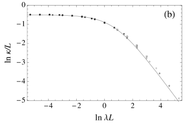
In Fig. 1 we show results for $\kappa$ as a function of $L$, for both $\lambda=0$ and $\lambda\neq 0$ (several values). When $\lambda=0$ we see clearly that $\kappa\propto L$, which means that we recover the ballistic results of Ref. rieder67. In fact, these results can even be compared with their exact solution. This is so because, due to our choice of potential, when $\lambda=0$ the $x$ and $y$ directions are independent, so that the heat conductivity is simply twice the original result for the one-dimensional chain. When $\lambda\neq 0$ we find that as $L$ increases, $\kappa$ tends to a finite value. The rapidity with which this asymptotic limit is reached increases with increasing $\lambda$. Notwithstanding, we may conjecture that irrespective of how small $\lambda$ is, in the thermodynamic limit ($L\to\infty$) this asymptotic value is always reached. This seems reasonable from the results of Fig. 1 and will also be corroborated by further arguments to be given below. Fig. 2 illustrates the dependence of $\kappa$ on $\lambda$ for different values of $L$. Note the broad range covered by $\lambda$, from $10^{-4}$ to $10^{2}$. This is a consequence of the efficiency of the numerical method just discussed. Fig. 2 shows that, when $L\to\infty$, $\kappa\propto 1/\lambda$.

Figure 1: Thermal conductivity $\kappa$ as a function of the system size $L$ for different values of $\lambda$, the intensity of the elastic collisions: from top to bottom, $\lambda=0$, 0.01, 0.05, 0.1, 0.5 and 1. The calculations are for the potential $U_{1}$ in Eq. (10) with fixed $k=1$, $\gamma=1$, $T_{A}=1$ and $T_{B}=2$.

Figure 2: $1/\kappa$ vs. $\lambda$ for different values of $L$: from top to bottom $L=5$, 10, 20, 50, 100, 200, 500 and 1000. The calculations are for the potential $U_{1}$ in Eq. (10) with the same parameters as in Fig 1.

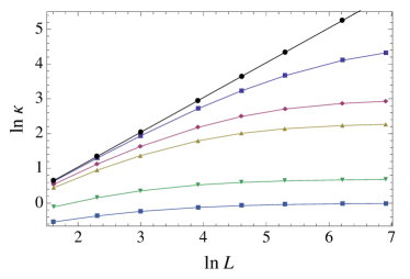
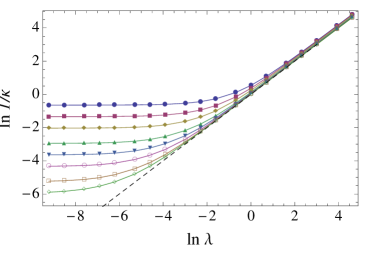
In summary, from Figs. 1 and 2 we find the following scaling behaviour: when $L\to\infty$, $\kappa\propto 1/\lambda$ and when $\lambda=0$, $\kappa\propto L$. We therefore assume the following scaling law landi13:

$$\kappa=\frac{a^{\prime}L}{b^{\prime}+\lambda L},$$ (36)

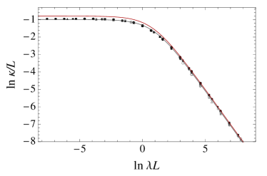
valid for small values of $\lambda$ and large values of $L$. A fitting of this finite-size scaling is presented in Fig. 3 where the collapse of the data points can be clearly observed. The finite-size scaling formula (36) clearly shows that $\lambda$ is a relevant parameter: as long as $\lambda\neq 0$, in the thermodynamic limit we always obtain a finite value of $\kappa$.

Figure 3: Finite size scaling of $\kappa/L$ vs. $\lambda L$ for the potential $U_{1}$, Eq. (10), with parameters $k=1$, $\gamma=1$, $T_{A}=1$ and $T_{B}=2$. The lower continuous line is a fitting to the data points from Eq. (36) with parameters $a^{\prime}$ and $b^{\prime}$. The upper continuous line represents the solution (39).

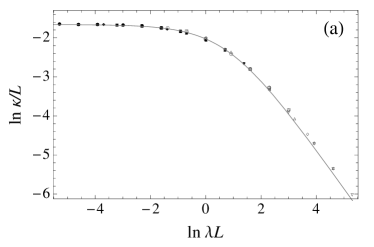
For completeness, in Fig. 4 we also present the scaling behaviour obtained for the other potentials, $U_{2}$ and $U_{3}$, defined in Eqs. (II) and (14) respectively. The parameters $a^{\prime}$ and $b^{\prime}$ in Eq. (36) were fitted to the data. As can be seen, a very similar behaviour is obtained, which corroborates our claim that the choice of potential is unimportant in obtaining Fourier’s law.

Figure 4: Finite size scaling of $\kappa/L$ vs. $\lambda L$ for the potentials (a) $U_{2}$ (with $\alpha=0.5$) and (b) $U_{3}$ (with $k^{\prime}=1$) in Eqs. (II) and (14). The solid line represents a fit from Eq. (36) with fit parameters $a^{\prime}$ and $b^{\prime}$. The other parameters are $k=1$, $\gamma=1$, $T_{A}=1$ and $T_{B}=2$.

IV Analytical results

IV.1 Symmetric and uncoupled potential

We now return to Eqs. (31) for the covariances under the potential $U_{1}$ and show how it can be simplified. Written explicitly, equation (31) gives $Z^{\dagger}=-Z$ and rCl (AZ-ZA)+(ΓY+YΓ) + 2λ(Y-¯Y) &= D,
(A X -X A) - (ZΓ+ ΓZ) = 2λZ,
2Y - (X A + A X) - (ZΓ- ΓZ) =0, where we have dropped the indices in $X_{1}$, $Y_{1}$ and $Z_{1}$.

Here we reach a remarkable result. These equations are exactly the same equations for the covariances in the velocity-flipping model, equation (7) of reference dhar11, which may therefore be interpreted as a particular case of our velocity-rotation model. It is important to note, however, that the fact that the equations for the covariances coincide does not imply that both models are identical. For instance, the equations governing the evolution of the probability distribution of both models are entirely different, which can be seen by noting that in the present model it is described by a standard Fokker-Planck equation, whereas in the velocity-flipping model the conserving noise is modelled by a master equation-type term dhar11. The fact that both models give the same equations for the covariances and, hence, that both lead to Fourier’s law, means that the rather sharp nature of the velocity-flipping model landi13; dhar11 is not the relevant ingredient to induce Fourier’s law. What is in fact relevant is the energy-conserving nature of the noise.

We begin our analysis by subtracting the equilibrium solution $X^{e}$, $Y^{e}$ and $Z^{e}$ from the covariance matrices $X$, $Y$ and $Z$. Recall that the non-vanishing elements of $D$ are $D_{11}=2\gamma T_{A}$ and $D_{LL}=2\gamma T_{B}$. The equilibrium covariances $X^{\rm e}$ and $Y^{\rm e}$ are solutions of rCl (ΓY^e+Y^eΓ) &= D^0,
(A X^e -X^e A) = 0,
2Y^e - (X^e A + A X^e) =0, where $D^{0}$ is the $L\times L$ diagonal matrix with nonvanishing elements $D^{0}_{11}=D^{0}_{LL}=2\gamma T$ and $T=(T_{A}+T_{B})/2$. Notice that the velocity-velocity covariance matrix $Y^{e}$ is diagonal and the position-velocity covariances vanish, $Z^{e}=0$.

Next we define the dimensionless matrices $X^{*}$, $Y^{*}$ and $Z^{*}$ by rCl X &= X^e + X*ΔTγ2,
Y = Y^e + Y^* ΔT,
Z = Z^e + Z*ΔTλ, where $\Delta T=T_{B}-T_{A}$. The equations for $X^{*}$, $Y^{*}$ and $Z^{*}$ are obtained by subtracting the equilibrium solution (IV.1)-(IV.1) from (IV.1)-(IV.1). Let us work with dimensionless quantities $A^{\prime}$ and $\Gamma^{\prime}$ defined by $A=kA^{\prime}$ and $\Gamma=\gamma\Gamma^{\prime}$. We also define $d$ as the diagonal matrix with elements $d_{11}=1$ and $d_{LL}=-1$. As a result we obtain the set of equations rCl εν(A’Z^*-Z^*A’)+(Γ’ Y^*+ Y^*Γ’) + 2ε (Y^*-¯Y^*) &= d,
ν(A’ X^* -X^* A’) -ε(Z^*Γ’ + Γ’ Z^*) = 2 Z^*,
ν(A’ X^*+X^* A’) + ε(Z^*Γ’ - Γ’ Z^*) =2Y^*, where $\nu=k/\gamma^{2}$ and $\varepsilon=\gamma/\lambda$ are now the only two free dimensionless parameters. As before, $\bar{Y}^{*}$ is the diagonal matrix formed by the diagonal elements of $Y^{*}$. These equations do not involve neither $T_{A}$ nor $T_{B}$ which shows that $X^{*}$, $Y^{*}$ and $Z^{*}$ do not depend on temperature. Now, from equation (12) and from the definition of the covariance $Z$ we see that the heat flux is $J=2kZ_{n,n+1}=2kZ^{*}_{n,n+1}\Delta T/\lambda$ from which we may write the following relation for the heat conductivity

$$\kappa=\frac{2kLZ^{*}_{n,n+1}}{\lambda}.$$ (37)

Since $Z^{*}$ does not depend on temperature we conclude that the heat conductivity does not depend on temperature. This result is valid for any harmonic potential and is a direct consequence of the linearity of the equations for the covariances rieder67.

It is worth mentioning an important property concerning the position-velocity covariances. If we consider the diagonal elements of the left and right-hand sides of equation (IV.1) we get the following result

$$Z^{*}_{12}=Z^{*}_{23}=\ldots=Z^{*}_{L-1,L}$$ (38)

which reflects the invariance of the heat flux along the chain and shows that $\kappa$, given by (37), does not depend on $n$, as it should. It also reflects the conservation of energy inside the chain. Incidentally, in the original harmonic chain rieder67, which is obtained from our model by setting $\lambda=0$, the matrix $Z$ is Toeplitz and Eq. (38) is thus fulfilled. When $\lambda\neq 0$, even though the first diagonal is still constant, as in Eq. (38), the same is not true of the others.

IV.2 Large $\lambda$ expansion

As will be shown in this section, the heat conductivity in the limit of large $\lambda$ and large $L$ is described by

$$\kappa=\frac{kL}{\frac{k}{\gamma}+c\gamma+\lambda L},$$ (39)

where $c$ is found numerically to be $c=1.20938909(5)$. We call the attention to the fact that, in the thermodynamic limit, $\kappa=k/\lambda$ and the heat conductivity is thus independent of the coupling constant $\gamma$. Formula (39) is depicted by the upper continuous line in Fig. 3. As can be seen, it agrees quite well with the simulations when $\lambda L$ is large. The agreement, as is expected, becomes worse when $\lambda L$ is small.

The purpose of this section is to derive formula (39) for the heat conductivity, valid for large $L$ and large $\lambda$. Exact expressions for the heat conductivity $\kappa$, Eq. (37), can be obtained by exactly solving equations (IV.1)-(IV.1) for small chains. As shown in the appendix, the results always have the same form of a ratio of polynomials in $\lambda$, in which the numerator is a polynomial of one order less than the denominator. The results obtained for small chains, from $L=2$ up to $L=14$, show that when $\lambda$ is large, the heat conductivity has the form

$$\kappa=\frac{kLS_{L}}{\frac{k}{\gamma}S_{L}+\gamma C_{L}+\lambda L}.$$ (40)

where $S_{L}$ and $C_{L}$ are rational numbers that depend on $L$. In the appendix we show the exact values of these numbers for $L=2$ up to $L=5$. Next we shall show that this formula is in fact valid for any $L$ and that $S_{L}$ and $C_{L}$ approach finite values, $S_{L}\to 1$ and $C_{L}\to c$, when $L\to\infty$, thus recovering Eq. (39).

We start by considering the solution of equations (IV.1)-(IV.1) for large $\lambda$ or, what is equivalent, small $\varepsilon$. We shall therefore assume that $X^{*}$, $Y^{*}$ and $Z^{*}$ can be written as a series expansion in $\varepsilon$ of the form rCl X^* &= X^0 + εX^I + ε^2 X^II + …,
Y^* = Y^0 + εY^I + ε^2 Y^II + …,
Z^* = Z^0 + εZ^I + ε^2 Z^II + …, Since $\kappa$ is given by Eq. (37), we may also write

$$\kappa=\kappa^{I}\varepsilon+\kappa^{II}\varepsilon^{2}+\ldots,$$ (41)

where

$$\kappa^{I}=\frac{2kL}{\gamma}Z^{0}_{n,n+1},\qquad\kappa^{II}=\frac{2kL}{\gamma}Z^{I}_{n,n+1}$$ (42)

Thus, our goal now is to find the functions $Z^{0}_{n,n+1}$ and $Z^{I}_{n,n+1}$.

Let us write down the ensuing equations for each order of $\varepsilon$ that stem from Eqs. (IV.1)-(IV.1). In order $1/\varepsilon$ the only contribution is found in Eq. (IV.1) and gives

$$Y^{0}=\bar{Y}^{0},$$ (43)

i.e., $Y^{0}$ is diagonal. To order zero in $\varepsilon$ we find the following system of equations: rCl (Γ’ Y^0 + Y^0 Γ’) + 2 (Y^I - ¯Y