Twisting solar coronal jet launched at the boundary of an active region

Abstract

Aims. A broad jet was observed in a weak magnetic field area at the edge of active region NOAA 11106 that also produced other nearby recurring and narrow jets. The peculiar shape and magnetic environment of the broad jet raised the question of whether it was created by the same physical processes of previously studied jets with reconnection occurring high in the corona.

Methods. We carried out a multi-wavelength analysis using the EUV images from the Atmospheric Imaging Assembly (AIA) and magnetic fields from the Helioseismic and Magnetic Imager (HMI) both on-board the SDO satellite, which we coupled to a high-resolution, nonlinear force-free field extrapolation. Local correlation tracking was used to identify the photospheric motions that triggered the jet, and time-slices were extracted along and across the jet to unveil its complex nature. A topological analysis of the extrapolated field was performed and was related to the observed features.

Results. The jet consisted of many different threads that expanded in around 10 minutes to about $100$ Mm in length, with the bright features in later threads moving faster than in the early ones, reaching a maximum speed of about 200 km s^-1. Time-slice analysis revealed a striped pattern of dark and bright strands propagating along the jet, along with apparent damped oscillations across the jet. This is suggestive of a (un)twisting motion in the jet, possibly an Alfvén wave. Bald patches in field lines, low-altitude flux ropes, diverging flow patterns, and a null point were identified at the basis of the jet.

Conclusions. Unlike classical $\lambda$ or Eiffel-tower shaped jets that appear to be caused by reconnection in current sheets containing null points, reconnection in regions containing bald patches seems to be crucial in triggering the present jet. There is no observational evidence that the flux ropes detected in the topological analysis were actually being ejected themselves, as occurs in the violent phase of blowout jets; instead, the jet itself may have gained the twist of the flux rope(s) through reconnection. This event may represent a class of jets different from the classical quiescent or blowout jets, but to reach that conclusion, more observational and theoretical work is necessary.

1 Introduction

Solar coronal jets were first identified in X-rays using data from the Soft X-ray Telescope (SXT; Tsuneta et al. 1991) on-board the Japanese mission Yohkoh. A statistical study determined that their typical length is $\approx$ few times $10^{4}$– $4\times 10^{5}$ km, the width $5\times 10^{3}$–$10^{5}$ km, the apparent average velocity around 200 km s^-1, and the lifetime from a few minutes to ten hours (Shimojo et al., 1996). Another analysis of 100 X-ray jets determined the magnetic configurations at the base of the jets: 8% of the jets occur in a single magnetic polarity, 12% in bipoles, 24% in mixed polarities, and 48% in a satellite polarity (Shimojo et al., 1998). The thermal parameters of jet plasma were intensively studied by Shimojo & Shibata (2000), who found the correlation between the temperatures of the jets and the sizes of the flares at the footpoints. Surges are observed in chromospheric spectral lines with a brightening at their base. Ultraviolet (UV) and X-ray jets may be associated with surges. Some attempts have been made at correlating X-ray jets and surges (e.g., Schmieder et al., 1995; Canfield et al., 1996). It was shown that cold and hot plasma exist along different magnetic field lines. The energy and temperature of the jet plasma were found to be related to the intensity of micro-flares.

More recently, some space-borne missions, such as TRACE, STEREO, and Hinode, have provided high resolution observations of jets in a multi-wavelength range with many components. Type II spicules with high velocities were detected in the Ca II line with the Solar Optical Telescope (SOT) onboard Hinode and were found to be associated with velocity jets observed with the Extreme-ultraviolet Imaging Spectrometer (EIS) on the same satellite. McIntosh & De Pontieu (2009) proposed that these combined jets provide enough energy to heat the coronal plasma. Ugarte-Urra & Warren (2011) analyzed jets at the periphery of active regions in cool (Si VII) and hot (Fe XII) lines observed with Hinode/EIS and concluded that the hot and cold plasmas are not directly related to one another. More powerful jets have been observed with data from the X-Ray Telescope (XRT) onboard Hinode with high kinetic energies (Cirtain et al., 2007; Savcheva et al., 2007). Jets and surges are often associated with micro-flares and X-ray bright points (Schmieder et al., 1995; Mandrini et al., 1996), with anemone-shaped configurations for coronal loops (Shibata et al., 1992; Zhang et al., 2012). Some of the observed jets display helical features that may be interpreted as associated with untwisting field line motions (e.g., Patsourakos et al., 2008; Shen et al., 2011; Chen et al., 2012).

The observed features as well as previous theoretical considerations (Heyvaerts et al., 1977) indicated that jets are caused by magnetic reconnection, which led to the first dynamical model, in two spatial dimensions, in which the reconnection was driven by flux emergence (Yokoyama & Shibata 1995, 1996; Nishizuka et al. 2008). At present, X-ray or EUV jets are being modeled in three dimensions, with the jets resulting either from the interaction of an emerging magnetic bipole with the preexisting coronal field (Moreno-Insertis et al., 2008; Archontis & Hood, 2012; Moreno-Insertis & Galsgaard, 2013) or from the effect of horizontal photospheric motions onto a simple null-point configuration in the atmosphere (Pariat et al., 2009a, 2010), with, in all those cases, an open magnetic field in the background corona. In both types of models, the jet is a consequence of the reconnection taking place in a current sheet at the interface between the perturbed and preexisting magnetic domains. The current sheet contains at least one null point and, as shown by Moreno-Insertis & Galsgaard (2013), may have a complex topology, including plasmoids. Formation of null points in the corona has also been shown by Török et al. (2009) using a zero-$\beta$ MHD simulation: the interface between an emerging twisted flux tube and a pre-existing arcade contains a null-point with associated reconnection that leads to a torsional Alfvén wave and the development of a sheared loop system.

Of particular interest is the recent identification of a subclass of X-ray and EUV jets called blowout jets (Moore et al. 2010; Sterling et al. 2010; see also Liu et al. 2011; Madjarska 2011). This class shows a first phase with a regular quiescent jet, followed by a violent flux-rope eruption at its base, whereby cool material at chromospheric or transition region temperatures is ejected, perhaps a cool rope as in a mini-CME eruption. An interpretation of this phenomenon has been offered recently (Moreno-Insertis & Galsgaard, 2013; Archontis & Hood, 2013) using the 3D flux-emergence models cited above. In the first of those references, the base of a quiescent jet becomes unstable and causes a collection of several flux rope ejections through different mechanisms (tether-cutting reconnection, kink instability) occurring in different parts of the emerged-field domain below the jet, which links that model with previous MHD simulations of the tether-cutting instability (Manchester et al., 2004; Archontis & Hood, 2012) or of the kink instability (Török & Kliem, 2003) in coronal flux ropes.

Of the various fundamental questions that are still open concerning X-ray / EUV jets in the solar corona, this paper is related with the following ones:

• are there structural differences between jets occurring within coronal holes, and jets that take place at their boundary, or at the boundary of active regions?

• are blowout jets a distinct subclass of X-ray / EUV jets, or do most quiescent jets develop a violent phase with flux rope eruptions toward the end of their lives? Vice versa: is there a class of jets consisting only of a violent flux rope ejection, that is, a blowout phase?

• Do all jets involve high-altitude magnetic reconnection occurring at chromospheric and coronal null points, or can the reconnection occur in other magnetic field configurations involving high spatial magnetic field gradients but no null points per se?

Regarding the last question, it is indeed known that coronal energetic events do not always involve three-dimensional null points. For example, X-ray bright points (Mandrini et al., 1996) and compact flares (Schmieder et al., 1997) can sometimes occur in quasi-separatrix layers (as defined in Démoulin et al., 1996). Also small flares (Aulanier et al., 1998; Pariat et al., 2004), chromospheric surges (Mandrini et al., 2002), and a recently studied recurring jet (Guo et al., 2013) have been related to bald patches (as defined in Bungey et al., 1996).

With those questions in mind, in this paper we study the evolution and the magnetic field configuration of a peculiar coronal jet that was observed by the Atmospheric Imaging Assembly (AIA; Lemen et al. 2012) onboard the Solar Dynamics Observatory (SDO). This event was peculiar in many respects. Firstly, SDO/AIA extreme-ultraviolet (EUV) observations revealed complex interleaved and broad emitting features, both along the jet itself and near its numerous footpoints. Secondly, the line-of-sight magnetic field observed by the Helioseismic and Magnetic Imager (HMI; Scherrer et al. 2012; Schou et al. 2012) onboard SDO showed that the jet was launched from a weak-field area surrounded by strong network polarities resulting from the decaying phase of the active region (AR11106). The jet itself cannot be unambiguously assigned to the quiescent or blowout types, and there is no clear hint of ejection of a flux rope as a mini-CME. We present the observations and our data analysis in Section 2. A nonlinear force-free field extrapolation and topology analysis of the event is given in Section 3. Finally, in Section 4, we summarize and discuss the results in the context of the aforementioned questions.

2 Observations and data analysis

2.1 AIA and HMI instruments

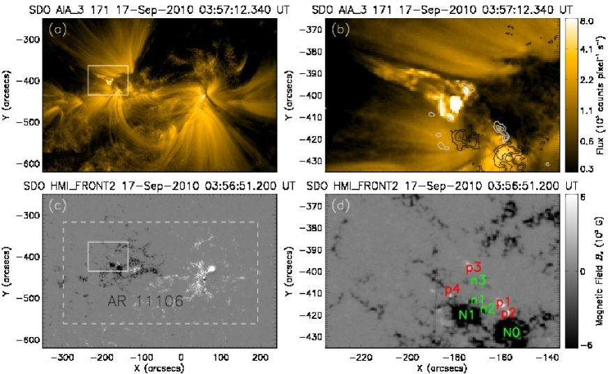
Figure 1: SDO/AIA 171 Å image and SDO/HMI line-of-sight magnetic field. (a) A jet in 171 Å observed by SDO/AIA at 03:57 UT. The solid box indicates the field of view of panels (b) and (d). (b) The same 171 Å image as that in panel (a) but in a smaller field of view. Gray/black lines represent positive/negative polarities of the line-of-sight magnetic field as shown in panels (c) and (d). The contour levels of $B_{\mathrm{LOS}}$ are -1200, -900, -600, 50, 300, and 600 G. (c) Line-of-sight magnetic field of the active region observed by SDO/HMI at 03:56 UT. The solid box is the same as in panel (a). The dashed box indicates the field of view used for removing the 180^∘ ambiguity and the projection effect. (d) The same line-of-sight magnetic field as in panel , but in a smaller field of view. Mixed parasitic polarities are denoted by p1, p2, p3, and p4 for positive polarities and n1, n2, and n3 for negative polarities. N0 and N1 denote the main negative polarities in the following part of the active region.

SDO/AIA provides filtergrams in seven EUV spectral lines and three UV-visible continuums with high cadence (12 s) and high spatial resolution ($1.5^{\prime\prime}$). Each of its four CCD arrays has $4096\times 4096$ pixels and the pixel sampling is $0.6^{\prime\prime}$. The field of view is $41^{\prime}$ x $41^{\prime}$, hence fully including a disk of radius $1.3\,R_{\odot}$. Due to its large spectral coverage, SDO/AIA observes the solar atmosphere over a large temperature range from the cold photosphere at about 5000K (white light and 1700 Å) to the hot active corona at around 10MK (94 Å , 131 Å and $193$ Å).

SDO/HMI observes the polarimetric line profiles at Fe I 6173 Å with a filter and two CCDs on the full disk of the Sun. Each of the two CCDs has $4096\times 4096$ pixels. The spatial resolution is $1^{\prime\prime}$ with a pixel size of $0.5^{\prime\prime}$. As a filtergraph, SDO/HMI scans the spectral line profile at six positions. The full width at half maximum (FWHM) of the filter is 76 mÅ and the spacing of the filter position is 69 mÅ. The two CCDs record two sets of data for computing the line-of-sight and vector magnetic field, respectively. For the first case, only the $I\pm V$ ($I$ and $V$ stands for the Stokes parameters) filtergrams at the six wavelengths are recorded, and the cadence is about 45 s. For the second case, four additional filtergrams ($I\pm Q$ and $I\pm U$, where $Q$ and $U$ stand for the other two Stokes parameters) at each of the six wavelengths are recorded, and the cadence is about 135 s. The Stokes parameters $I,Q,U$ and $V$ are computed from the raw data after necessary calibrations. However, to increase the signal-to-noise ratio, the Stokes parameters are averaged over 12 minutes. The vector magnetic fields are derived using the code very fast inversion of the Stokes vector (VFISV; Borrero et al. 2011).

2.2 EUV jet and line-of-sight magnetic field

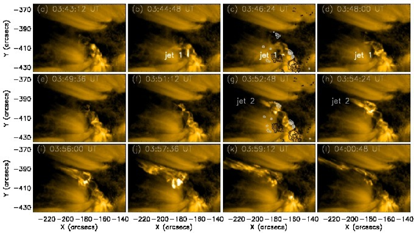
Figure 2: SDO/AIA 171 Å images showing the evolution of two EUV jets. The color scale is the same as in Figure 1. The labels jet 1 and jet 2 denote the two jets close to each other both in time and space. Grey/black lines in panels (c) and (g) represent positive/negative polarities of the line-of-sight magnetic field at 03:56:51 UT. The contour levels of $B_{\mathrm{LOS}}$ are -1200, -900, -600, 50, 300, and 600 G.

Many bright points and jets (around 30) were observed in the eastern and western edges of active region (AR) 11106 on September 17, 2010. We focus our study on the main jets occurring in the following (eastern) polarity of AR 11106, where Guo et al. (2013) studied three major recurring jets, whose SDO/AIA 171 Å flux peaked at 03:17, 03:57 and 04:22 UT, respectively. From Figures 2 and 5 of Guo et al. (2013), they found that the 171 Å flux curve around 03:57 UT shows some smaller peaks before the main peak, while the other two events at 03:17 and 04:22 UT have only one peak. The 03:57-UT jet is labeled Jet 2  in the following while the recurrent jets studied by Guo et al. (2013) are collectively called Jet 1. One of those jets occurs close in space and time to Jet 2, but the parasitic polarities involved in Jet 1 and Jet 2 are different, as we show below. The detailed evolution and magnetic configuration of the peculiar event at 03:57 UT we call Jet 2 have not been studied yet and constitute the object of the present paper. Figure 1a shows large-scale coronal loops connecting the two main polarities in AR 11106 observed with SDO/AIA 171 Å. A coronal jet is present at the east (left) edge of AR 11106. The footpoints of the jet are located at some parasitic positive polarities, as shown in Figure 1b and d.

AR 11106 survived for several solar rotations. It mainly consisted of a dispersed magnetic field on each side of a large filament channel, which can be seen as the dark lane in Figure 1a below the large-scale coronal loops. This active region was observed in August, September, October, and November in 2010. In September, there was still a leading positive polarity spot and the following polarity was mainly formed by intense network polarities of kilo Gauss strength (Figure 1c). Inside the following negative polarity, emerged continuously bipoles. The main emergence occurred on 2010 November 9, when a new active region was formed inside the remnant region. On 2010 September 17, there were two locations of positive polarities in the following negative polarity region in the intra-network (Figure 1c). We focus on the northeast one shown in the solid box of Figure 1c. The polarities correspond to the emergence of bipoles occurring one or two days before. On September 17, the active region was close to the central meridian.

In Figure 1d, we present a small field of view concentrating on the following part of the active region with two main polarities labeled N0 and N1 ($B_{\mathrm{LOS}}>1000$ G). Weaker mixed polarities ($B_{\mathrm{LOS}}$ of about 100 to 600 G) are inside a supergranule identified in the dispersed magnetic field of the active region. It is surrounded by negative polarities (N0 and N1 to the nouth of the supergranule). There are many parasitic polarity regions corresponding to different systems of emerging flux, for example, p1–n1, p2–n2, and p3–n3.

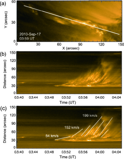
Figure 3: (a) EUV jet observed with the 171 Å filter of SDO/AIA on 17 September 2010. The solid line indicates the slit position along which the jet was ejected. (b) Temporal evolution of the 171 Å image in the slice along the jet. (c) Some linear fitted lines overlaid on the time-slice 171 Å image. As time passes, different components or kernels of the jet were launched from the jet base with increasing speed, reaching 200 km s^-1.

Figure 2 shows the evolution of the EUV jets in 171 Å from 03:43 to 04:00 UT. Only bright points can be seen at 03:43 UT, as shown in Figure 2a. At 03:44 UT, a small curved jet (Figure 2b through d) appeared above the parasitic polarities p1–n1 and p2–n2. We labeled this Jet 1. It extended toward the southeast and lasted until 03:48 UT. At 03:51 UT (Figure 2f), a small jet emanating from p3 began to the north of Jet 1. The jet (Jet 2) extended toward the east with some brightening kernels at its footpoint in the west end (Figure 2g). Later on (Figures 2h, 2i, and 2j), we find many threads along the jet and some brighter kernels at its basis. At 03:59 UT (Figure 2k), the jet was composed of about ten threads with an angle of about 10 to 20 degrees aligned in the direction of the ejection. The global shape of the jet looks like the Eiffel Tower and it consists of different branches with seemingly torsional threads. The number of bright threads decreased at 04:00 UT (Figure 2l) while the remaining long thread still increased in size and speed. Jet 2 disappeared at about 04:08 UT.

Jet 2 was also clearly observed in other filters of SDO/AIA, for example, 304 Å, 193 Å, 221 Å, and 1600 Å. The jet had many thermal components that not completely co-spatial. Between 03:34 to 03: 41 UT, the jet was visible as a dark structure in absorption in the 304 Å filter, which indicates a surge-like behavior. Some brightenings were detected at the jet base in 1600 Å. The jet was also observed in soft X-rays with Hinode/XRT.

2.3 Time-Slice analysis of the EUV jet

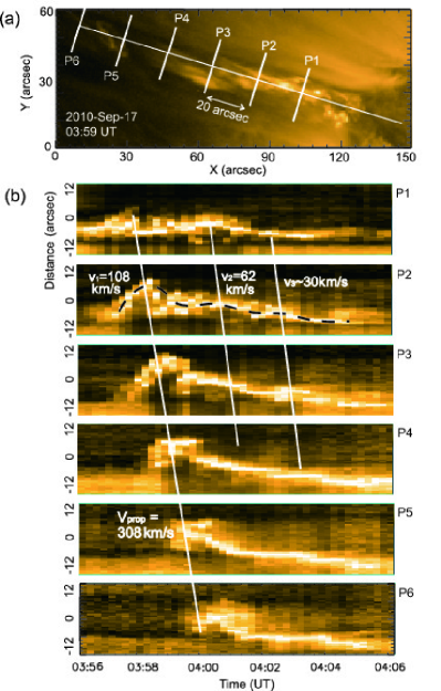
Figure 4: (a) EUV jet observed with the 171 Å filter of SDO/AIA on 17 September 2010. The shorter solid lines indicate the slit positions at six different heights used for (b), which are perpendicular to the longer solid line. The length of the slits is $24^{\prime\prime}$. (b) Time-distance diagram of the 171 Å EUV jet along the slits at the six different heights. The dashed black line shows the oscillation pattern at one height, and the white lines indicate the propagation velocity of the oscillation patterns at different heights.

To quantify the propagation of the jet, we made a time-slice analysis. First, we selected a straight line (called a slit in the following) roughly along the jet on the 171-Å SDO/AIA image, as shown in Figure 3a. Next, we drew the brightness distribution along the slit for successive times with the aim to discern the propagation of features in the jet (Figure 3b, c). In the figure we see that some bright features started to rise at around 03:49 UT with a speed of 54 km s^-1. Presently, a striped pattern of dark and light lines or strands becomes apparent; the pattern extends to higher values of the ordinates as time passes. The pattern suggests the propagation of a wave motion; it would be compatible with the signal left by untwisting field lines carrying the hot material, or, more generally, with an Alfvén wave propagating along twisted field lines. However, some other mechanisms would also account for it, such as intermittent ejections of plasmoids along straight field lines or successive plasma ejections along sheared field lines. Moreover, because the 171 Å emission is optically thin, it is impossible to determine the chirality of any twist of the field lines involved in this emission pattern (see also the discussion in Section 3). As time passes, different components or kernels of the jet are launched from the base with increasing speeds, reaching in projection $200$ km s^-1. They reach a projected length of 100 Mm. This indicates that the EUV jet was becoming more dynamical during this phase of its life, perhaps as a result of the relaxation of a twisted structure. This speed is comparable with the results of other authors (Cirtain et al., 2007; Patsourakos et al., 2008). As said in Sec. 2.2, the jet was also observed with Hinode/XRT (with temperature of around a few million degrees). The spatial resolution is lower and the determination of the jet speed has a large error. Nevertheless, the increase in velocity was also observed.

To study the evolution of the jet plasma that is perpendicular to the propagation direction, we made a fishbone-slit cut as shown in Figure 4a. Six slits were selected perpendicular to the jet propagation direction. The distance between each pair of adjacent slits is $20^{\prime\prime}$. The 171 Å intensity distribution along each of the six slits is arranged as a function of time in Figure 4b, with panels labeled P1 through P6. Any apparent vertical motion in these panels thus corresponds to sideways elongation of the bright features in Figure 4a away from the main axis of the jet. In each of the six slits, we find that the bright features moved basically along the whole length of the P1 - P6 transverse slits. We also discern a time shift between the patterns seen in successive panels, from P1 through P6: we have drawn slanted white straight lines to indicate this shift. Additionally, there is an apparent swing or oscillation in the motion of the main bright feature in panels P1 - P3: we have drawn a solid dashed black curve in P2 to highlight this apparent phase motion. The dashed dark curve seems to indicate a damped oscillation taking place sideways of the main jet axis. We found three periods of oscillation and the numbers above the curve denote the amplitude of the corresponding velocity, namely $108$ km s^-1, $62$ km s^-1, and $30$ km s^-1, respectively, with an error estimated to be around 10 km/s. This may indicate that the oscillation is triggered in the initial phase, slowly decaying thereafter.

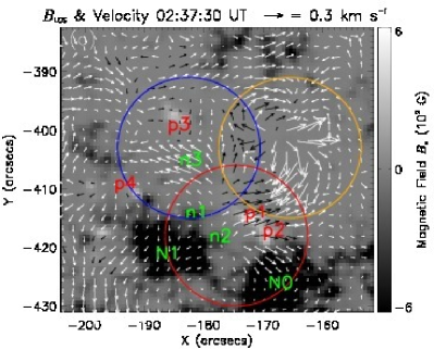
Figure 5: Photospheric transverse velocity derived through LCT analysis of the SDO/HMI magnetograms. The background is the average line-of-sight magnetic field with positive (white) and negative (black) polarities. Arrows represent the transverse velocity, where black/white is located on the positive/negative polarity. The time interval for averaging the line-of-sight magnetic field is 02:25–02:50 UT.

2.4 Evolution of the line-of-sight magnetic field

To study the transverse flows of photospheric magnetic features, we employed the local correlation tracking technique (LCT; November & Simon 1988). A Gaussian tracking window with a full width at half maximum (FWHM) of $5^{\prime\prime}$ was adopted. A time series of 137 SDO/HMI magnetograms starting at 02:00 UT on 2010 September 17 and with a cadence of 45 seconds was used for the analysis. All the magnetograms were aligned with each other prior to the LCT analysis. We refer to Guo et al. (2013) for detailed descriptions on the alignment. Then, the magnetograms were grouped and averaged in $25$-minute series to decrease the noise. The transverse velocity maps were derived by the LCT technique with the averaged magnetograms. They were finally trimmed to include only the area present in all frames.

Figure 5 contains one of the LCT velocity maps obtained in that process. The figure shows strong diverging and converging velocity distributions. We selecedt three regions in the map (indicated with circles in red (bottom), orange (top right), and blue (top left) ) to investigate the flow patterns in detail. In the region enclosed by the red circle, the weak polarities p1–n1 and p2–n2 continuously emerged in the intra-network and moved at a speed of $\sim 0.2$ km s^-1 toward the preexisting main polarities N0 and N1 at the edge of the supergranule. The opposite polarities within each of the pairs p1–n1 and p2–n2 move-away from each other, which suggests they were emerging bipoles. The magnetic polarity p2 moves toward N0. This polarity pattern has been interpreted as an instance of emerging flux causing the jet series called Jet 1 (Guo et al., 2013).

For the region enclosed by the blue circle (top left) toward the center of Figure 5, we see a cluster of negative polarities, which we call n3, moving toward the northeast (upper left), in the direction of polarities p3 and p4. This is the location from which jet 2 is launched.

In the third region, indicated in Figure 5 by an orange circle (top right), a diverging flow pattern with a clockwise rotation is apparent. The velocity vectors are discontinuous in the common area of this circle with either the blue or the red ones. The velocity arrows near the orange-red intersection are directly opposite, and we see in the orange-blue one a rotational shear. We show in Sec. 3.2 that there are bald patches in these intersections and, generally, in the interior of the orange circle; there is also an extended bald patch to the north-east of the blue circle.

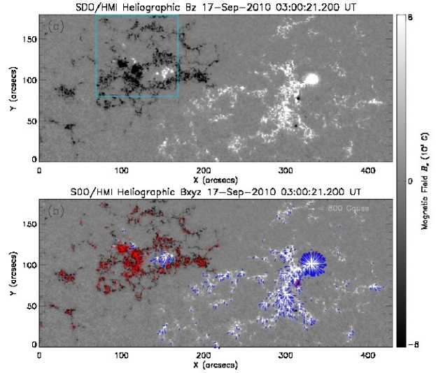
Figure 6: (a) Grayscale map of the vertical component of the vector magnetic field in the domain used for the NLFFF extrapolation (the field strength is indicated in the vertical bar on the right). The field strength shown in the figure is corrected from the projection effects but has not yet been subjected to preprocessing. The solid box marks the region used in later sections to compute the bald patches and to plot magnetic field lines. (b) Vertical and horizontal components of the vector magnetic field. The direction and length of the arrows indicate the direction and strength of the horizontal magnetic field, respectively. For the conversion from arrow length to field strength, a sample arrow is shown in the upper right corner.

3 NLFFF extrapolation and topology analysis

3.1 Vector magnetic field and NLFFF extrapolation

For the extrapolation, we used the photospheric vector magnetic field data obtained through SDO/HMI as described in Section 2.1. For the following analysis we used the data corresponding to 03:00 UT. The transverse components of the vector magnetic field suffer from a $180^{\circ}$ ambiguity, which was removed with the improved version of the minimum-energy method (Metcalf, 1994; Metcalf et al., 2006; Leka et al., 2009). Then, we corrected for the projection effects with the method proposed by Gary & Hagyard (1990). The correction was carried out in two steps. First, the line-of-sight and transverse components of the vector magnetic field were transformed to the heliographic components. Then, these fields were projected from the image plane on to the plane tangential to the solar surface at the center of the selected field of view. In this case, the center is located at $x=-60.0^{\prime\prime}$ and $y=-439.5^{\prime\prime}$ at 03:00 UT. Correction of the projection effects is necessary since the region of interest is located at a relatively high latitude in the southern hemisphere. After the correction, any fake polarities associated with the projection disappear. The corrected vector magnetic field is shown in Figure 6.

To derive the three-dimensional magnetic field configuration, we extrapolated the photospheric boundary data assuming the field to be force-free, that is by solving the equations $\nabla\times\mathbf{B}=\alpha\mathbf{B}$ and $\nabla\cdot\mathbf{B}=0$. The pseudo-scalar $\alpha$ must be constant along individual field lines (as follows from combining the two equations), but otherwise needs not be constant in space. The de-projected vector magnetic field was used as the bottom boundary condition (bc); the boundary conditions on the other boundaries of the cubic box were set by using the results of a potential field extrapolation of the vertical component of the photospheric boundary data. The resulting problem is nonlinear, and we select the optimization method (Wheatland et al., 2000; Wiegelmann, 2004; Wiegelmann & Inhester, 2010) to obtain the solution.

A requirement for successful NLFFF modeling is that the net magnetic flux on the photospheric boundary must be near zero, that is the flux of the positive and negative magnetic patches in the boundary data approximately balance. In practice, this condition requires that the photospheric vector data used for the NLFF modeling include all strong positive and negative magnetic flux concentrations of the AR, and that the latter are sufficiently far from the boundaries of the selected subfield (DeRosa et al., 2009). Only then do the field lines issuing from the strongest flux and electric current concentrations reconnect to the lower boundary of the NLFF model field and one can reasonably assume to have properly captured the magnetic connectivity within the active region. For our de-projected observational boundary data (shown in Figure 6), the flux-balance parameter, which is defined as the absolute value of the ratio of the net signed vertical magnetic flux over the total unsigned vertical magnetic flux, is $0.034$, that is, it is nearly flux balanced.

In addition, the force-free assumption for the magnetic field in a given volume leads to specific conditions for the field on the boundary of the volume related to the Lorentz force itself and to its torque (Aly, 1989); in our case, these conditions are unlikely to be satisfied, not even approximately, by the observational boundary data, -specially because the plasma $\beta$ is not low at the photosphere (Metcalf et al., 1995; Tiwari, 2012). To solve this problem, Wiegelmann et al. (2006) proposed a preprocessing of the boundary data. The method has four input parameters, $\mu_{1},\mu_{2},\mu_{3}$, and $\mu_{4}$, which regulate the quality of the boundary condition resulting from the preprocessing concerning not only the zero-force and -torque conditions, but also the closeness to the observed data and the smoothing. The method leads to a decrease of the dimensionless magnetic force parameter from $0.420$ to $0.001$ before and after the preprocessing, respectively, and of the dimensionless torque parameter from $0.400$ to $0.002$. As noted by Wiegelmann et al. (2006), vector maps with dimensionless force and torque parameters on the order of $10^{-2}$ can validly be used as input for the NLFFF magnetic modeling. The flux balance parameter becomes $0.038$ due to the preprocessing, that is, it remains equally low.

The preprocessed vector magnetic fields were then used as boundary input in the improved optimization method of Wiegelmann & Inhester (2010) to obtain a solution of the NLFFF problem. The improved algorithm relaxes the magnetic field not only in the volume but also in the lower boundary of the cubic computational domain. We followed the prescriptions provided by Wiegelmann et al. (2012) concerning the weighting and injection speed of the lower-boundary data. The extrapolation was performed in a cubic box resolved by $860\times 360\times 680$ grid points. As an indication of the quality of the magnetic field obtained, we mention that the average angle between the magnetic field and the electric current density is about $10.6^{\circ}$.

3.2 Magnetic topology of Jet 2

Coronal jets are widely accepted to be the consequence of magnetic reconnection, which often occurs in magnetic structures with singular topologies, such as null-points with their associated fan-spine configurations (Pontin, 2011). On the other hand, magnetic reconnection is also possible in Quasi-Separatrix-Layers (QSLs), which, in fact, may account for the launching of the jet complex (Jet 1) studied by Guo et al. (2013). QSLs are likely to appear associated with bald patches (as discussed below). To understand the structure of the jet analyzed in the present paper (Jet 2), we therefore aimed at locating the possible null points and bald patches in the area of interest where the jet has its roots.

Magnetic dips are magnetic field lines that are concave in their upper part. The magnetic field at the bottom of magnetic dips fulfills the conditions $\mathbf{B}\cdot\nabla B_{z}>0$ and $B_{z}=0$, with $z$ the upward-pointing vertical coordinate. Bald patches are magnetic dips whose bottom touches the photosphere. With this definition, the bald patches were computed and are shown by the small green circles in Figure 7. They all lie along the polarity inversion line, shown as a thin olive-green line. The small dark-red circles in the figure mark the foot points of the field lines that are tangential to the bald patches. To facilitate identification, we have repeated in the figure the blue circle of Figure 5. To the west (i.e., right) of the blue circle, we see a collection of bald-patch lines associated with the p1 and p2 positive polarities located above the strong negative polarity labeled N0. These bald patches are situated in the interior of the orange circle of Figure 5. The closeness in space of these bald-patch lines and their different orientations reflect how complicated the field line structure is in that region. We traced the magnetic connectivity of these bald patches using the NLFFF extrapolation data. Most of the field lines going through them just end up connecting to the main positive polarity of the active region via simple large-scale loops. However, as one moves in the region toward the north, field lines connecting to the roots of the jet begin to appear. The bald-patch region near the right boundary of (but still inside) the blue circle is particularly interesting: this is the region of high-velocity shear in Figure 5; the field lines traced from that region connect in part to the jet area and in part to the positive AR polarity, with strong field-orientation changes. It is clear that important field-line shear is taking place there.

Back in Figure 7, we see another extended bald-patch line to the north-east (i.e., top-left) of the blue circle. These bald patches are associated with the weak positive polarity p3 (which appears as a small magenta ring within the circle). We show presently that this region has a complicated and interesting topology, with very different large-scale connectivity patterns for neighboring patches, which can also explain part of the reconnection that causes Jet 2.

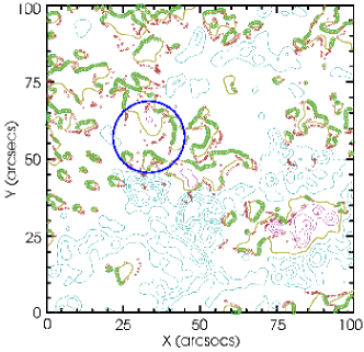
Figure 7: Bald patches (green circles) computed from the NLFFF field model. Dark red circles represent the footpoints of the bald patch field lines. Magenta/cyan solid lines denote the contours of the positive/negative polarity. The olive-green solid line indicates the polarity inversion line, where all the bald patches are located. The blue circle in this figure is the same as shown in Figure 5 and marks the region from where Jet 2 is launched.

  

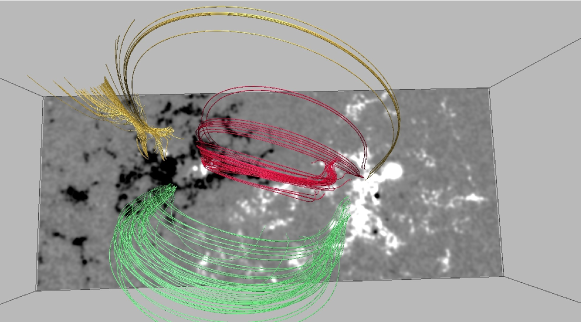
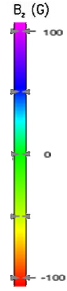
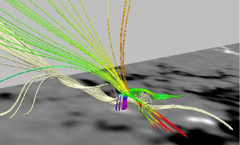
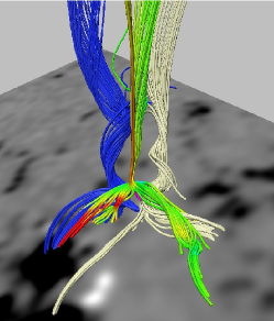
Figure 8: Field line connectivities obtained through the NLFFF extrapolation. Top panel: the green and red field line sets illustrate the general connectivity between the main polarities of AR11106 and resemble structures visible in the SDO/AIA image of Figure 1. The yellow field lines are traced from the region at the base of the jet and clearly reproduce the geometry of the latter. Lower panels: local and remote connectivities of the region around the minor positive polarity p3. One of the field line sets is colored according to the value of $B_{z}$, the colorscale follows the color bar on the left. The ivory and royal-blue field line sets show twisted flux ropes on either side of the central spine.

Figure 8 (top panel) illustrates the large-scale connectivity pattern of various patches on the negative side of the active region, including the supergranule on the north-east (top-left) that contains the positive polarities p1-p2 and p3 (compare this figure with Figure 1; the supergranule is contained in the small rectangle of panels a and c in that figure). The coronal loops drawn in green and red in the top panel of Figure 8 roughly correspond to bright SDO/AIA loops seen to be rooted toward the lower right corner of the rectangle in Figure 1a. On the other hand, at the top-left corner of Figure 8 (still in the top panel) we see a complex field-line connectivity pattern above polarity p3 (yellow field lines) that roughly coincides in location, shape, and orientation with the complex bright structure at the base of jet 2 visible in Figure 1a and b. Closer inspection (Figure 8, bottom-left panel) illustrates some of the topological features of the field above the p3 polarity. The panel shows two sets of field lines; in one of them the color of the line varies with the sign and magnitude of the vertical component of the magnetic field following the rainbow colors, as given in the color bar on the left. Color saturation is reached at $|B_{z}|=100$ G. This set of field lines reveals a singular structure similar to a highly asymmetric null point at a height of some $3.5$ Mm above p3. The incoming field lines include a spine-like axis linking the structure to p3 on the surface (purple field lines descending to the white patch on the surface) and, on the top side, field lines that come from the high levels of the box (colored in pale green or blue). The outgoing field lines are issued almost horizontally and link the structure to the negative polarities at the periphery of the supergranule. At the center of this structure is a deep minimum of the magnetic field strength, which can be identified with a null point within the accuracy of the NLFFF extrapolation. A linear analysis of the magnetic field structure around that point reveals three real eigenvalues of the field gradient matrix, one of which is much lower in absolute value than the other two: this confirms the highly asymmetric character of the null. There are more structures of interest in this domain: the vertical spine axis linking downward to p3 is flanked on its NW and SE sides by two highly inclined (i.e., not far from horizontal) flux ropes. One of them (the one to the NW) is shown in the panel with field lines in ivory: this rope has a left-handed twist. The other flux rope has field lines with a right-handed twist and is located to the SE of the spine; it can be seen (deep-blue field lines) in the bottom-right panel of Figure 8, which shows that site from a different perspective. The two flux ropes extend toward the north-east of the FOV roughly in the direction of Jet 2.

The topological relation of the structures just described in the neighborhood of polarity p3 with the bald patches to the north-east of it is illustrated in Figure 9. The horizontal plane in both panels contains a superposition of the NLFFF magnetogram (as also used in Figure 8) and the diagram of Figure 7, including the blue circle: the two panels contain the same field line sets, viewed from different perspectives. Three field line bunches have been drawn (in yellow, gray and light magenta) that become tangential to the photosphere approximately at the location of different bald patches to the north-east of p3. For better identification with the previous figure, the set of field lines around the singular structure visible in Figure 8 is also repeated here, with the same color-code along them.

Combining the information of Figures 8 and 9, we conclude that Jet 2 is launched from a region at the edge of AR 11106, where strong gradients of connectivity (QSLs) appear: patches connected with the strong positive polarity of the active region sit next to domains which connect with the open field outside of it. Moreover, the intrusion of positive polarities into a supergranule with the predominant polarity of that side of the active region causes a collection of bald patches and a very asymmetric null point to appear. This is clearly a region well suited for reconnection. A simple hypothesis is, then, that Jet 2 is associated with reconnection linked to this topological complexity.

4 Discussion

The observational characteristics of the present jet, combined with its coronal magnetic field environment as derived from the NLFFF extrapolation, pose a real challenge for an interpretation in terms of the classical jet models. In the following we discuss separate aspects of the jet that can provide some guidance in relation to the questions posed in the introduction.

4.1 Reconnection at multiple sites that leads to the jet

The jet studied in this paper seems to be launched from a variety of sites in the boundary area between the large-scale closed active-region loops and the open field outside. The particular region on which we focused our analysis is the supergranule highlighted in the rectangle of Figure 1. The photospheric field in this supergranule is predominantly of negative polarity, but has a number of weaker positive-polarity intrusions in its interior. The result, as shown in Sec. 3.2, is a complicated field line geometry and topology. We located (a) several bald patches with field lines connected with the jet region; (b) a singular point similar to an asymmetric null point that is connected to all important domains in the active region (and in the supergranule itself) and (c) two large, highly-inclined twisted flux ropes located on either side of the lower spine of the null-point structure and with opposite helicity sign. We believe that reconnection associated with these structures is the initial cause for the jet and its various strands.

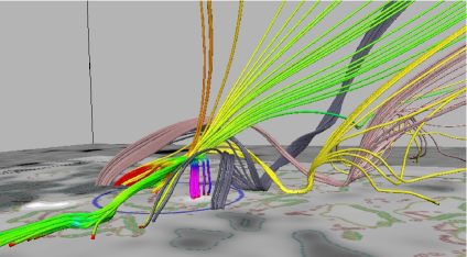
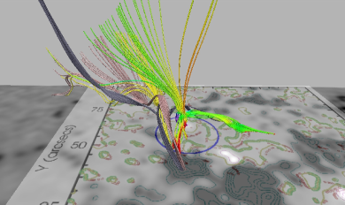
Figure 9: Visualization of three field line sets that go through the bald patches to the north-east of p3 (in dark gray, yellow, and light magenta). The two panels show different perspectives of the same field lines. The bottom plane contains a superposition of the NLFFF magnetogram and the image of Figure 7. To facilitate identification, the field line set visible in the bottom panels of Figure 8 that is colored according to the value of $B_{z}$ is repeated here.

The reason why the NLFFF displays several bald patches is that the sparse photospheric small flux concentrations (p3, p4 and n1, n2) in which the coronal jet is apparently rooted were actually located in the middle of a supergranule, where the ambient vertical flux density was weak. Additionally, a significant part (but not all) of the remote connectivity of the supergranule interior is done with the field in the outskirts of the active region, which has a substantial inclination from the vertical direction here. This roughly horizontal field was stronger in magnitude than that of the small flux concentrations like p3 or p4. The latter, then, cause small perturbations to this ambient field. The p3 positive polarity was strong enough to produce a deep minimum of the field strength above itself, which can be identified with a null point with real eigenvalues. No other singular structures of null-point type were found in the region, there is an abundance of bald patches in it. The remaining remote connectivity of the supergranule interior is with the positive polarity of the active region via tall coronal loops: in fact one sees in neighboring patches a mixture between the two types of remote connectivity (to the AR positive polarity or to the field in the outskirts of the active region, respectively). This is particularly the case of the topology near p3, as shown in Figure 8, bottom-left panel.

Therefore, while we cannot pinpoint any individual separatrix layer at a specific location as directly responsible for the reconnection that leads to the jet, we argue that the appearance of the weaker positive polarities in the supergranule interior and the general horizontal motions in the supergranule, as exemplified in the LCT map of Figure 5, may have generated electric currents at the separatrices (see Low & Wolfson 1988, Billinghurst et al. 1993, Pariat et al. 2009b), until the jet reconnection eventually started, in particular related to the p3 positive polarity with its neighboring bald patches in the north-east and west. The fact that the jet has several components that start at different times and propagate at different velocities (as is clear from the time-slice analysis along the jet in 171 Å) is an indication that different reconnection sites were sequentially activated during the event, probably because several of them were linked by some common field lines. On the other hand, the similarity between the field-line geometry shown in Figures 8 and 9 and the general shape of Jet 2 apparent in Figure 1 supports the assumption that the field-line sets and structures identified in Section 3.2 are directly associated with the jet, in spite of the uncertainty of the magnetic field inversion results used in this study (especially in weak field-regions) and the general limitations of NLFF modeling.

4.2 Conversion of flux ropes into torsional Alfvén waves

Different recent observations of X-ray or EUV jets, referred to in Sect. 1, have revealed the occurrence of (un)twisting motions at high altitude along the jets (the first of which was Patsourakos et al., 2008). These have been interpreted as the propagation of a torsional Alfvén wave generated by the reconnection between large-scale loops and low-lying twisted fields (firstly by Pariat et al. 2009a, then confirmed by Török et al. 2009). Suggestions of MHD waves propagating along jets have also been provided by Nishizuka et al. (2008). But thus far direct evidence of magnetic twist existing before the observed launch of jets has been elusive; a possible exception is the work of Sun et al. (2012), but in their case the twisted coronal field lines actually erupted all together, as in the mini-CME eruptions reported for the violent phase of the blowout jets (as in Moore et al., 2010; Sterling et al., 2010). From the point of view of theory, the eruption of twisted ropes seems to be a natural process occurring in the aftermath of a quiescent jet ejection: twisted ropes created at the base of the jet erupt through a variety of mechanisms, thus bringing twisted field lines to higher levels (Moreno-Insertis & Galsgaard, 2013; Archontis & Hood, 2013), thereby possibly providing an explanation for the blowout-jet phenomenon.

The jet studied in this paper seems to share common elements with both the quiescent and violent phases of the blowout-jet phenomenon. The broad nature of the jet and its transient undulatory transverse motions (as shown in the 171 Å time-slice plots across the jet of Sec. 2.3) are suggestive of the propagation of (possibly torsional) Alfvén waves. The NLFFF extrapolation offers a natural explanation for the generation of these waves. The two highly inclined flux ropes on either side of the positive flux patch p3 discussed in Sec. 3.2 must have been created in relation to the formation of that positive polarity itself (as corresponds to the opposite signs of the helicity in these ropes). The field lines in the ropes are actually rooted in different regions of the supergranule interior; in the other direction, they are part of the outward-going field lines at the AR periphery. The reconnection creating the ropes then must lead to a twist imbalance between the ropes’ low- and high-altitude sections. This will subsequently lead to the upward propagation of a torsional Alfvén wave. Depending on the circumstances, the ropes themselves may erupt, or, alternatively, all or most of their pre-eruptive twist may be carried away with the torsional wave and the ropes do not erupt. This means that this jet may have features corresponding to the two phases of the blowout-jet phenomenon.

Observationally, however, there is no definitive evidence for any of the possibilities just mentioned. On the positive side, the pre-event corona around the footpoints of the jet does show complex 171 Å emission patterns varying on a much smaller spatial scale than where large coronal loops can be seen. But these patterns cannot be indisputably attributed to the presence of a small-scale low-lying flux rope. In addition, we do not see a clear flux-rope-eruption-like signature in the event.

We therefore conjecture that the strength and orientation of the ambient magnetic field in a region where a jet is launched following the appearance of new magnetic polarities has a strong effect on the nature and on the observational characteristics of the jet (as previously shown for a simple configuration by Galsgaard et al. 2007). For instance, if the contrast of orientations between ambient field and emerging flux is high enough and the latter has sufficient field strength and total flux, a coronal null point may result and the jet may be of the type described by the three dimensional numerical models mentioned in the introduction. On the other hand, if the orientation contrast is not too strong and/or the emerging field is too weak, a bald patch may result and the reconnection may be mostly associated with the latter structure, possibly in the lower part of the corona. Also, if a strong-enough horizontal flux rope with sufficient twist is initially present, one can obtain an eruption as in the violent phase of the blowout jets. But if the flux rope is too weak, it will be converted into a torsional wave by reconnection, which will thus result in a classical untwisting jet.

The foregoing results raise a number of questions concerning the generality of the jet-launching mechanisms that lie at the basis of the event analyzed in this paper. From the theoretical point of view, the necessity and mutual influence of flux emergence, organization of the field in bald-patch regions, creation of the flux ropes, etc. in causing the jets can only be understood from a time-evolution analysis of a complex region. Observationally, one can only ascertain the generality of this type of jets as a separate class via a statistical analysis of coronal and photospheric data. These are natural extensions of this work that go beyond the objectives of the current paper.