Innermost Stable Circular Orbits and Epicyclic Frequencies Around a Magnetized Neutron Star

Abstract

A full-relativistic approach is used to compute the radius of the innermost stable circular orbit (ISCO), the Keplerian, frame-dragging, precession and oscillation frequencies of the radial and vertical motions of neutral test particles orbiting the equatorial plane of a magnetized neutron star. The space-time around the star is modelled by the six parametric solution derived by Pachón et al. It is shown that the inclusion of an intense magnetic field, such as the one of a neutron star, have non-negligible effects on the above physical quantities, and therefore, its inclusion is necessary in order to obtain a more accurate and realistic description of the physical processes occurring in the neighbourhood of this kind of objects such as the dynamics of accretion disk. The results discussed here also suggest that the consideration of strong magnetic fields may introduce non-negligible corrections in, e.g., the relativistic precession model and therefore on the predictions made on the mass of neutron stars.

1 Introducction

Stellar models are generally based on the Newtonian universal law of gravitation. However, considering the size, mass or density, there are five classes of stellar configurations where one can recognize significant deviations from the Newtonian theory, namely, white dwarfs, neutron stars, black holes, supermassive stars and relativistic star clusters (Misner et al.,, 1973). In the case of magnetized objects, such as white dwarfs ($\sim 10^{5}~{}$T) or neutron stars ($\sim 10^{10}~{}$T), the Newtonian theory not only fails in describing the gravitational field generated by the matter distribution, but also in accounting for the corrections from the energy stored in the electromagnetic fields.

Despite this fact and due to the sheer complexity of an in-all-detail calculation of the gravitational and electromagnetic fields induced by these astrophysical objects, one usually appeals to approaches based on post-Newtonian corrections (Aliev & Özdemir,, 2002; Preti,, 2004), which may or may not be enough in order to provide a complete and accurate description of the space-time around magnetized astrophysical objects. In particular, these approaches consider, e.g., that the electromagnetic field is weak compared to the gravitational one and therefore, the former does not affect the space-time geometry (Aliev & Özdemir,, 2002; Preti,, 2004; Mirza,, 2005; Bakala et al.,, 2010, 2012). That is, it is assumed that the electromagnetic field does not contribute to the space-time curvature, but that the curvature itself may affect the electromagnetic field. Based on this approximation, the space-time around a stellar source is obtained from a simple solution of the Einstein’s field equations, such as Schwarzschild’s or Kerr’s solution, superimposed with a dipolar magnetic field (Aliev & Özdemir,, 2002; Preti,, 2004; Mirza,, 2005; Bakala et al.,, 2010, 2012). Although, to some extend this model may be reliable for weakly magnetized astrophysical sources, it is well known that in presence of strong magnetic fields, non-negligible contributions to the space-time curvature are expected, and consequently on the physical parameters that describe the physics in the neighbourhood of these objects.

In particular, one expects contributions to the radius of the innermost stable circular orbit (ISCO) (Sanabria-Gómez et al.,, 2010), the Keplerian frequency, frame-dragging frequency, precession and oscillation frequencies of the radial and vertical motions of test particles (Bakala et al.,, 2010, 2012; Stella & Vietri,, 1999), and perhaps to other physical properties such as the angular momentum of the emitted radiation (Tamburini et al.,, 2011), which could reveal some properties of accretion disks and therefore of the compact object (Bocquet et al.,, 1995; Broderick et al.,, 2000; Konno et al.,, 1999; Cardall et al.,, 2001). In other words, to construct a more realistic theoretical description that includes purely relativistic effects such as the modification of the gravitational interaction by electromagnet fields, it is necessary to use a complete solution of the full Einstein-Maxwell field equations that takes into account all the possible characteristics of the compact object. In this paper, we use the six parametric solution derived by Pachón et al., (2006) (hereafter PRS solution), which provides an adequate and accurate description of the exterior field of a rotating magnetized neutron star (Pachón et al.,, 2006, 2012), to calculate the radius of the ISCO, the Keplerian, frame-dragging, precession and oscillation frequencies of neutral test-particles orbiting the equatorial plane of the star. The main purpose of this paper is to show the influence of the magnetic field on these particular quantities.

The paper is organized as follows. In section 2, we briefly describe the physical properties of the PRS solution, the general formulae to calculate the parameters that characterize the dynamics around the star are presented in section 3. Sections 4 and 5 are devoted to the study of the influence of the magnetic field on the ISCO radius and on the Keplerian and epicyclic frequencies, respectively. The effect of the magnetic field on the energy $E$ and the angular momentum $L$ is outlined in section 6. Finally, the conclusions of this paper are given in section 7.

2 Description of the Space-Time Around the Source

According to Papapetrou, (1953), the metric element $ds^{2}$ around a rotating object with stationary and axially symmetric fields can be cast as

$$ds^{2} =-f(dt-\omega d\phi)^{2}+f^{-1}[e^{2\gamma}(d\rho^{2}+dz^{2})+\rho^{2}d\phi^{2}],$$

where $f$, $\gamma$ and $\omega$ are functions of the quasi-clyndrical Weyl-Papapetrou coordinates $(\rho,z)$. The non-zero components of metric tensor, which are related to the metric functions $f$, $\omega$ and $\gamma$, are

$$g_{\phi\phi} =\frac{\rho^{2}}{f(\rho,z)}-f(\rho,z)\omega(\rho,z)^{2},\qquad g_{tt}=-f(\rho,z),$$ (1)

$$g_{t\phi} =f(\rho,z)\omega(\rho,z),\qquad g_{zz}=g_{\rho\rho}=\frac{{\rm e}^{2\gamma(\rho,z)}}{f(\rho,z)}=\frac{1}{g^{zz}}=\frac{1}{g^{\rho\rho}}.$$ (2)

By using the Ernst procedure and the line element in equation (2), it is possible to rewrite the Einstein- Maxwell equations in terms of two complex potentials ${\cal{E}}(\rho,z)$ and $\Phi(\rho,z)$ [see Ernst, (1968) for details]

$$({\rm Re}\,{\cal E}+|\Phi|^{2})\nabla^{2}{\cal E} = (\nabla{\cal E}+2\Phi^{*}\nabla\Phi)\cdot\nabla{\cal E},$$

$$({\rm Re}\,{\cal E}+|\Phi|^{2})\nabla^{2}\Phi = (\nabla{\cal E}+2\Phi^{*}\nabla\Phi)\cdot\nabla\Phi\,,$$ (3)

where ^∗ stands for complex conjugation. The above system of equations can be solved by means of the Sibgatullin integral method (Sibgatullin,, 1991; Manko & Sibgatullin,, 1993), according to which the Ernst potentials can be expressed as

$${\cal E}(z,\rho)=\frac{1}{\pi}\int_{-1}^{1}\frac{e(\xi)\mu(\sigma)d\sigma}{\sqrt{1-\sigma^{2}}},\qquad\Phi(z,\rho)=\frac{1}{\pi}\int_{-1}^{1}\frac{f(\xi)\mu(\sigma)d\sigma}{\sqrt{1-\sigma^{2}}}\,,$$

where $\xi=z+\mathrm{i}\rho\sigma$ and $e(z)={\cal E}(z,\rho=0)$ and $f(z)=\Phi(z,\rho=0)$ are the Ernst potentials on the symmetry axis. As shown below, these potentials contain all information about the multipolar structure of the astrophysical source [see also Pachón & Sanabria-Gómez, (2006) for a discussion on the symmetries of these potentials]. The auxiliary unknown function $\mu(\sigma)$ must satisfy the integral and normalization conditions

$$\mathchoice{{\vbox{\hbox{$\textstyle-$}}\kern-4.86108pt}}{{\vbox{\hbox{$\scriptstyle-$}}\kern-3.25pt}}{{\vbox{\hbox{$\scriptscriptstyle-$}}\kern-2.29166pt}}{{\vbox{\hbox{$\scriptscriptstyle-$}}\kern-1.875pt}}\!\int_{-1}^{1}\frac{\mu(\sigma)[e(\xi)+\tilde{e}(\eta)+2f(\xi)\tilde{f}(\eta)]d\sigma}{(\sigma-\tau)\sqrt{1-\sigma^{2}}}=0,\qquad\int_{-1}^{1}\frac{\mu(\sigma)d\sigma}{\sqrt{1-\sigma^{2}}}=\pi.$$ (4)

Here $\eta=z+i\rho\tau$ and $\sigma,\tau\in[-1,1]$, $\tilde{e}(\eta)=e^{*}(\eta^{*})$, $\tilde{f}(\eta)=f^{*}(\eta^{*})$.

For the PRS solution (Pachón et al.,, 2006), the Ernst potentials were chosen as:

$$e(z)=\frac{z^{3}-z^{2}(m+ia)-kz+is}{z^{3}+z^{2}(m-ia)-kz+is}\,,\qquad f(z)=\frac{qz^{2}+i\mu z}{z^{3}+z^{2}(m-ia)-kz+is}.$$ (5)

The electromagnetic and gravitational multipole moments of the source were calculate by using the Hoenselaers & Perjés method (Hoenselaers & Perjes,, 1990) and are given by (Pachón et al.,, 2006):

$$M_{0} =m,\quad M_{2}=(k-a^{2})m,...\qquad\hskip 11.09654ptS_{1}=a,\quad S_{3}=-m(a^{3}-2ak+s),...$$ (6)

$$Q_{0} =q,\quad Q_{2}=-a^{2}q-a\mu+kq,...\quad B_{1}=\mu+aq,...\quad B_{3}=-a\mu+\mu k-a^{3}q+2akq-qs,...$$ (7)

where the $M_{i}$s denote the moments related to the mass distribution and $S_{i}$s to the current induced by the rotation. Besides, the $Q_{i}$s are the multipoles related to the electric charge distribution and the $B_{i}$s to the magnetic properties. In the previous expressions, $m$ corresponds to the total mass, $a$ to the total angular moment per unit mass ($a$ = $J/M_{0}$, being $J$ the total angular moment), $q$ to the total electric charge. In our analysis, we set the electric charge parameter $q$ to zero because, as it is case of neutron stars, most of the astrophysical objects are electrically neutral. The parameters $k,\ s$ and $\mu$ are related to the mass quadrupole moment, the current octupole, and the magnetic dipole, respectively.

Using Eqs. (2) and (5), the Ernst potentials obtained by Pachón et al., (2006) are

$${\cal E}=\frac{A+B}{A-B}\,,\qquad\Phi=\frac{C}{A-B}\,,$$ (8)

which leads to the following metric functions:

$$f =\frac{A\bar{A}-B\bar{B}+C\bar{C}}{(A-B)(\bar{A}-\bar{B})}\,,\quad e^{2\gamma}=\frac{A\bar{A}-B\bar{B}+C\bar{C}}{\displaystyle{K\bar{K}\prod_{n=1}^{6}r_{n}}}\,,$$ (9)

$$\omega =\frac{{\rm Im}[(A+B)\bar{H}-(\bar{A}+\bar{B})G-C\bar{I}]}{A\bar{A}-B\bar{B}+C\bar{C}}.$$ (10)

The analytic expressions for the functions $A$, $B$, $C$, $H$, $G$, $K$, and $I$ can be found in the original reference (Pachón et al.,, 2006) or in Appendix of Pachón et al., (2012). A Mathematica 8.0 script with the numerical implementation of the solution can be found at http://gfam.udea.edu.co/$\sim$lpachon/scripts/nstars.

3 Characterization of the Dynamics Around the Source

In the framework of general relativity, the dynamics of a particle may be analyzed via the Lagrangian formalism as follows. Let us consider a particle of rest mass $\mathfrak{m}_{0}=1$ moving in a space-time characterized by the metric tensor $g_{\mu\nu}$, thus the Lagrangian of motion of the particle is given by

$${\cal L}=\frac{1}{2}g_{\mu\nu}\dot{x}^{\mu}\dot{x}^{\nu},$$ (11)

where the dot denotes differentiation with respect to the proper time $\tau$, $x^{\mu}(\tau)$ are the coordinates. Since the fields are stationary and axisymmetric, there are two constants of motion related to the time coordinate $t$ and azimuthal coordinate $\phi$ [see Ryan, (1995) for details], these are given by:

$$E=-\frac{\partial{\cal L}}{\partial\dot{t}}=-g_{tt}\bigg{(}\frac{dt}{d\tau}\bigg{)}-g_{t\phi}\bigg{(}\frac{d\phi}{d\tau}\bigg{)},$$ (12)

$$L=\frac{\partial{\cal L}}{\partial\dot{\phi}}=g_{t\phi}\bigg{(}\frac{dt}{d\tau}\bigg{)}+g_{\phi\phi}\bigg{(}\frac{d\phi}{d\tau}\bigg{)},$$ (13)

where $E$ and $L$ are the energy and the canonical angular momentum per unit mass, respectively. For real massive particle, the four velocity is a time-like vector with normalization $g_{\mu\nu}u^{\mu}u^{\nu}=-1$. If the motion takes place in the equatorial plane of the source $z=0$, this normalization condition leads to

$$g_{\rho\rho}\bigg{(}\frac{d\rho}{d\tau}\bigg{)}^{2}=-1+g_{tt}\bigg{(}\frac{dt}{d\tau}\bigg{)}^{2}+g_{\phi\phi}\bigg{(}\frac{d\phi}{d\tau}\bigg{)}^{2}+2g_{t\phi}\bigg{(}\frac{dt}{d\tau}\bigg{)}\bigg{(}\frac{d\phi}{d\tau}\bigg{)}.$$ (14)

From equation (14), one can identify an effective potential that governs the geodesic motion in the equatorial plane [see e.g. Bardeen et al., (1972)]

$$V_{\mathrm{eff}}(\rho)=1-\frac{E^{2}g_{\phi\phi}+2ELg_{t\phi}+L^{2}g_{tt}}{g^{2}_{t\phi}-g_{\phi\phi}g_{tt}}.$$ (15)

For circular orbits, the energy and the angular momentum per unit mass, are determined by the conditions $V_{\mathrm{\mathrm{eff}}}(\rho)=0$ and $dV_{\mathrm{eff}}/d\rho=0$. Based on these conditions, one can obtain expressions for the energy and the angular momentum of a particle that moves in a circular orbit around the star [see e.g. Stute & Camenzind, (2002)], namely,

$$E=\frac{\sqrt{f}}{\sqrt{1-f^{2}\chi^{2}/\rho^{2}}},\qquad L=E(\omega+\chi),$$ (16)

$$\chi=\left\{\rho[-\omega_{,\rho}f^{2}-\sqrt{\omega^{2}_{,\rho}f^{4}+f_{,\rho}\rho(2f-f_{,\rho}\rho)}\right\}/\left[f(2f-f_{,\rho}\rho)\right],$$ (17)

where the colon stands for a partial derivative respect the lower index. The radius of innermost stable circular orbit (ISCO’s radius) is determined by solving numerically for $\rho$ the equation

$$d^{2}V_{\mathrm{eff}}/d\rho^{2}=0,$$

which arising from the marginal stability condition. This condition together with the equations (16) and (17) can be write in terms of the metric functions as [see Stute & Camenzind, (2002)]

$$\omega_{,\rho}\omega_{,\rho\rho}f^{5}\rho(2f-f_{,\rho}\rho)+\omega^{2}_{,\rho}f^{4}\big{[}2f^{2}+(f_{,\rho\rho}f-f_{,\rho})\rho^{2}\big{]}+\omega_{\rho}f^{2}\sqrt{\omega^{2}_{,\rho}f^{4}+f_{,\rho}(2f-f_{,\rho}\rho)}\big{[}2f^{2}-f\rho(4f_{,\rho}+f_{,\rho\rho}\rho)$$

$$+2f^{2}_{,\rho}\big{]}+\rho(2f-f_{,\rho}\rho)\Big{[}3f_{\rho}f^{2}-4f^{2}_{,\rho}f\rho+f^{3}_{,\rho}\rho^{2}+f^{2}\big{[}f_{\rho\rho}\rho-\omega_{,\rho\rho}f\sqrt{\omega^{2}_{,\rho}f^{4}+f_{,\rho}(2f-f_{,\rho}\rho)}\big{]}\Big{]}\ =\ 0.$$ (18)

As is usual in the literature, the physical ISCO radius reported here corresponds to evaluation of $\sqrt{g_{\phi\phi}}$ at the root of equation (3). This equation is solved for fixed total mass of the star $M$, the dimensionless spin parameter $j=J/M^{2}$ (being $J$ the angular momentum), the quadrupole moment $M_{2}$ and the magnetic dipolar moment $\mu$ [see Table VI of Pappas & Apostolatos, (2012)].

3.1 Keplerian, Oscillation and Precession Frequencies

The Keplerian frequency $\Omega_{\mathrm{K}}$ at the ISCO can be obtained from the equation of motion of the radial coordinate $\rho$. This equation is easily obtained by using the Lagrangian (11),

$$g_{\rho\rho}\ddot{\rho}-\frac{1}{2}\Big{[}-g_{\rho\rho,\rho}\dot{\rho}^{2}+g_{\phi\phi,\rho}\dot{\phi}^{2}+g_{tt,\rho}\dot{t}^{2}+g_{t\phi,\rho}\dot{t}\dot{\phi}\Big{]} =0.$$ (19)

By imposing the conditions of circular orbit or constant orbital radius, $d\rho/d\tau=0$ and $d^{2}\rho/d\tau^{2}=0$ and taking into account that $d\phi/d\tau=\Omega_{K}dt/d\tau$, one gets [see e.g. Ryan, (1995)]

$$\Omega_{\mathrm{K}}=\frac{d\phi}{dt}=\frac{-g_{t\phi,\rho}\pm\sqrt{(g_{t\phi,\rho})^{2}-g_{\phi\phi,\rho}g_{tt,\rho}}}{g_{\phi\phi,\rho}},$$ (20)

where “$+$” and “$-$” denotes the Keplerian frequency for corotating and counter-rotating orbits, respectively.

The epicyclic frequencies are related to the oscillations frequencies of the periastron and orbital plane of a circular orbit when we apply a slightly radial and vertical perturbations to it. According to Ryan, (1995), the radial and vertical epicyclic frequencies are given by the expression

$$\nu_{\alpha} =\frac{1}{2\pi}\bigg{\{}-\frac{g^{\alpha\alpha}}{2}\bigg{[}(g_{tt}+g_{t\phi}\Omega_{k})^{2}\bigg{(}\frac{g_{\phi\phi}}{\rho^{2}}\bigg{)}_{,\alpha\alpha}$$

$$-2(g_{tt}+g_{t\phi}\Omega_{k})(g_{t\phi}+g_{\phi\phi}\Omega_{k})\bigg{(}\frac{g_{t\phi}}{\rho^{2}}\bigg{)}_{,\alpha\alpha}+(g_{t\phi}+g_{\phi\phi}\Omega_{k})^{2}\bigg{(}\frac{g_{tt}}{\rho^{2}}\bigg{)}_{,\alpha\alpha}\bigg{]}\bigg{\}},$$

where $\alpha=\{\rho,z\}$. The periastron $\nu_{\rho}^{\mathrm{p}}$ and the nodal $\nu_{z}^{\mathrm{p}}$ frequencies are defined by:

$$\nu^{\mathrm{p}}_{\alpha}=\frac{\Omega_{k}}{2\pi}-\nu_{\alpha},$$ (21)

which are the ones that have an observational interest (Stella & Vietri,, 1999). The radial oscillation frequency vanishes at the ISCO radius and therefore, the radial precession frequency equals to the Keplerian frequency.

Finally, the frame dragging precession frequency or Lense–Thirring frequency $\nu_{\mathrm{LT}}$ is given by [see e.g. Ryan, (1995)]

$$\nu_{\mathrm{LT}}=-\frac{1}{2\pi}\frac{g_{t\phi}}{g_{\phi\phi}}\ .$$ (22)

$\nu_{\mathrm{LT}}$ is related to purely relativistic effects only (Misner et al.,, 1973). In this phenomenon, the astrophysical source drags the test particle into the direction of its rotation angular velocity. In absence of electromagnetic contributions, as in the case of the Kerr solution, the frame dragging comes from the non-vanishing angular momentum of the source. In the presence of electromagnetic contributions in non-rotating sources, it was shown by Herrera et al., (2006) that the non-zero circulation of the Poynting vector is able to induced frame dragging, in which case it is electromagnetically induced. In the cases discussed below, due to the presence of fast rotations and magnetic fields, the frame dragging will be induced by a combination of these two processes.

4 Influence of the Dipolar Magnetic Field in the ISCO Radius.

As it was discussed in the Introduction, contributions from the energy stored in the electromagnetic fields come via equivalence between matter and energy, $E=mc^{2}$. For the particular case of a magnetar ($\sim 10^{10}~{}$T), the electromagnetic energy density is around $4\times 10^{25}~{}$J/m³, with an $E/c^{2}$ mass density $10^{4}$ times larger than that of lead. Hence, the relevant physical quantities should depend upon the magnetic field, and in particular on the magnetic dipole moment $\mu$.

Model	$M_{0}$ [km]	$j$	$M_{2}$ [km3]	$S_{3}$ [km4]
M17	4.120	0.588	-51.8	-210.0
M18	4.139	0.635	-62.6	-279.0
M19	4.160	0.682	-74.9	-365.0
M20	4.167	0.700	-79.8	-401.0

Table 1: Realistic numerical solutions for rotating neutron stars derived by Pappas & Apostolatos, (2012). Here, $M_{0}$ is the total mass of the star, $j$ is the dimensionless spin parameter: $j=J/M_{0}^{2}$ (being $J$ the angular momentum), $M_{2}$ is the quadrupole moment and $S_{3}$ is the current octupole moment [see Table VI of Pappas & Apostolatos, (2012)].

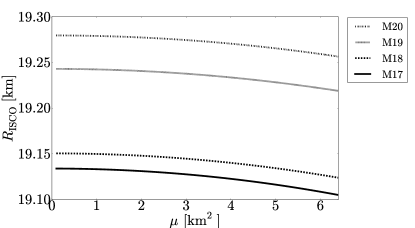
Figure 1: ISCO radius as a function of magnetic dipole parameter $\mu$. The physical parameters for the star correspond to the models M17-M20 listed in Table 1. An increase of $\mu$ leads to a decrease of the ISCO radius.

Figure 1 shows the ISCO radius as a function of the parameter $\mu$ for four particular realistic numerical solutions for rotating neutron stars models derived by Pappas & Apostolatos, (2012). The models used coincide with the models 17,18,19 and 20 of Table VI in that reference and correspond to results for the Equation of State L (see Table 1). The lowest multipole moments of the PRS solution, namely, mass, angular moment and mass quadrupole were fixed to the numerical ones obtained by Pappas & Apostolatos, (2012) (see Table 1). Since the main objective here is to analyze the influence of the magnetic dipole, the current octupole parameter $s$ was set to zero. Note that this does not mean that the current octupole moment vanishes (see in Eq. (6). The parameter $\mu$ was varied between $0$ and $6.4$ km², which corresponds to magnetic fields dipoles around $0$ and $6.3\times 10^{31}$ Am², respectively. In all these cases, the ISCO radius decreases for increasing $\mu$, this can be understood as a result of the dragging of inertial frames induced by the presence of the magnetic dipole, we elaborate more on this below.

5 Keplerian and Epicyclic Frequencies

Some of the predictions from General Relativity (RG) such as the dragging of inertial systems (frame-dragging or Lense-Thirring effect) (Everitt et al.,, 2011), the geodesic precession (geodesic effect or de Sitter precession) (Everitt et al.,, 2011) or the analysis of the periastron precession of the orbits (Lucchesi & Peron,, 2010) have been experimental verified. However, since they have observed in the vicinity of the Earth, these observations represent experimental support to RG only in the weak field limit. Thus, it is fair to say that the RG has not been checked in strong field limit [see e.g. Psaltis, (2008)]. In this sense, the study of compact objects such as black holes, neutron stars, magnetars, etc., is certainly a topic of great interest, mainly, because these objects could be used as remote laboratories to test fundamental physics, in particular, the validity of general relativity in the strong field limit yet (Stella & Vietri,, 1999; Pachón et al.,, 2012).

The relevance of studying the Keplerian, epicyclic and Lense-Thirring frequencies relies on the fact that they are usually used to explain the quasiperiodic oscilation phenomena present in some Low Mass X-ray Binaries (LMXRBs). In this kind of systems a compact object accretes matter form the other one (which is usually a normal star) and the X-ray emissions could be related to the relativistic motion of the accreted matter e.g. rotation, oscillation and precession. Stella & Vietri, (1999) showed that in the slow rotation regime, the periastron precession and the Keplerian frequencies could be related to the phenomena of the kHz quasiperiodic oscillations (QPOs) observed in many accreting neutron stars in LMXRBs (Stella & Vietri,, 1999). This model is known as the Relativistic Precession Model (RPM) (Stella & Vietri,, 1999) and identifies the lower and higher QPOs frequencies with the periastron precession and the keplerian frequencies respectively. The RPM model has been used to predict the values of the mass and angular momentum of the neutron stars in this kind of systems [see e.g. Stella & Vietri, (1999) and Stella et al., (1999), for details].

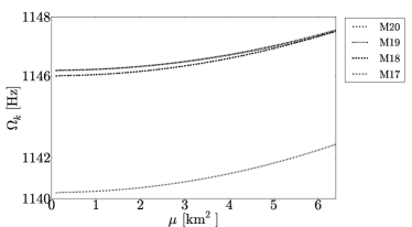
(a)

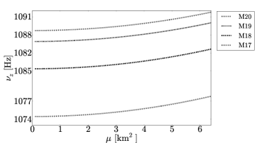
(b)

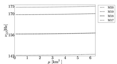
(c)

Figure 2: Keperian frequency (a), nodal precession frequency (b) and, Lense-Thirring frequency (c) as a function of the $\mu$ parameter. All the frequencies increase for increasing $\mu$.

In the framework of the RPM, it is assumed that the motion of the accretion disk is determined by the gravitational field alone and thereby, it is normal to assume that the exterior gravitational field of the neutron star is well described by the Kerr metric. However, most of the neutron stars have (i) quadrupole deformations that significantly differ from Kerr’s quadrupole deformation (Laarakkers & Poisson,, 1999) and (ii) a strong magnetic field. The influence of the non-Kerr deformation was discussed, e.g., by Johannsen & Psaltis, (2010) and Pachón et al., (2012). Based on observational data, it was found that non-Kerr deformations dramatically affect, e.g., predictions on the mass of the observed sources. Below, we consider the influence of the magnetic field and find that it introduces non-negligible corrections in the precession frequencies and therefore, on the predictions made by the Kerr-based RPM model.

In the previous section, it was shown that the magnetic field affects the value of the ISCO radius of a neutral test particle that moves around the exterior of a magnetized neutron star. Below it shown that other physicals quantities such as the Keplerian and epicyclic frequencies, which are used to describe the physics of accretion disk, are also affected. The influence on the Lense-Thirring frequency is also discussed.

Fig. 2 shows the influence of the magnetic field in the Keplerian [Fig. 2(a)], nodal precession [Fig. 2(b)] and Lense-Thirring [Fig. 2(c)] frequencies. In all cases, the frequencies are plotted as a function of the parameter $\mu$ while fixing the others free parameters (mass, angular moment and mass quadrupole) according to the realistic numerical solutions in Table 1. As it expected is for shorter ISCO radius (see previous section), all frequencies increase with increasing $\mu$. The changes in the Lense-Thirring frequency come from the electromagnetic contribution discussed above.

6 Energy and Angular Momentum

In order to understand the results presented above, we consider that it is illustrative to consider first the effect that the magnetic field has on the energy $E$ and the angular momentum $L$ needed to described marginally stable circular orbits [see equations (16) and (17)]. In doing so, we fix the total mass $M_{0}$, the spin parameter $j$ and the quadrupole moment $M_{2}$, according to the values in Table 1. Figures 3(a) and 3(b) show $E$ and $L$ at the ISCO as a function of the dipolar moment $\mu$. By contrast to the case of the Keplerian frequency, an increase of $\mu$ decreases the value of the energy and the angular momentum needed to find an ISCO. Complementarily, in figures 4(a) and 4(b), $E$ and $L$ are depicted as a function of $\rho$ for various values of the dipolar moment. Since the energy and the angular momentum associated to the ISCO correspond to the minima of the curves $E(\rho)$ and $L(\rho)$ (indicated by triangles), the figures show that an increase of the magnetic dipole moment induces a decrease of the ISCO radius (see Fig. 1 above) and simultaneously a decrease of the energy and the angular momentum.

At a first sight, for an increasing magnetic field, it may seem conspicuous that the angular momentum, of co-rotating test particles, decreases [see Fig. 4(b)] whereas the Keplerian frequency increases [see Fig. 2(a)]. However, this same opposite trend is already present in the dynamics around a Kerr source when the angular momentum of the source is increased [cf. equations (2.13) for the angular momentum and (2.16) for the Keplerian frequency in Bardeen et al., (1972)]. In Kerr’s case, the co-rotating test particles are dragged toward the source thus inducing a shorter ISCO radius [cf. equation (2.21) in Bardeen et al., (1972)], and since the leading order in the Keplerian frequency goes as $\sim 1/\rho^{2}$, a larger frequency is expected. By contrast, the contra-rotating test particles are “repelled” by the same effect thus resulting in an increase of the ISCO radius and in a decrease of the Keplerian frequency [see also Fig. 2 in Pachón et al., (2012)].

Having in mind the situation in Kerr’s case and by noting that the frame dragging can be induced by current multipoles of any order (Herrera et al.,, 2006), the goal now is to compare the characteristics of the contributions from the angular momentum and the dipole moment to the Keplerian frequency based on the approximate expansions derived by Sanabria-Gómez et al., (2010) and appeal then the general theory of multipole moments to track the contribution of dipole moment to the current multipole moments. If the expression for the Keplerian frequency [Eq. (21)] and for the angular momentum [Eq. (23)] in Sanabria-Gómez et al., (2010) are analyzed in detail, one finds that the signs of the contributions of the angular momentum and the magnetic dipole of the source coincide, this being said, one could argue that the contribution of the dipole moment is related to an enhancement of the current multipole moment of the source. This remark is confirmed by the general multipole expansion discussed by Sotiriou & Apostolatos, (2004). In particular, the influence of the dipole moment in the higher current-multipole moments is clear from Eq. (23)–(25) of this reference.

Hence, the role of the dipole moment of the source in the dynamics of neutral test particles is qualitatively analogous to the role of the angular momentum, albeit it induces corrections of higher orders in multipole expansion of the effective potential. This is a subject that deserves a detailed discussion and will be explained somewhere else.

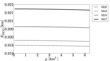
(a)

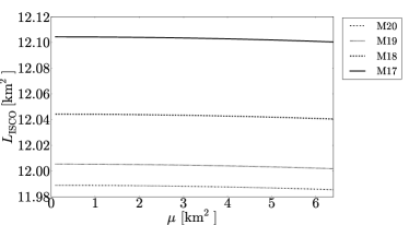
(b)

Figure 3: Energy (a) and angularmomentum (b) of a test particle at the ISCO radius versus magnetic dipole parameter $\mu$ given by the PRS solution. We can see that reduction of the energy and angular momentum of the particle while the the magnetic dipole of the star is increased.

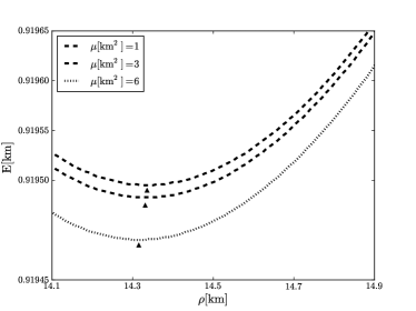
(a)

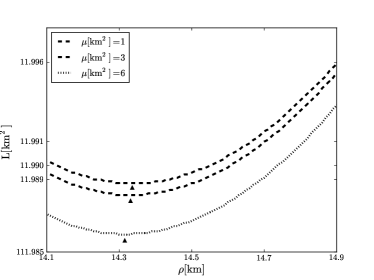
(b)

Figure 4: Energy (a) and angular momentum (b) of a test particle at the ISCO radius versus magnetic dipole parameter $\mu$ given by the PRS solution. We can see that reduction of the energy and angular momentum of the particle while the the magnetic dipole of the star is increased.

7 Concluding Remarks

The influence of weak electromagnetic fields on the dynamics of test particles around astrophysical objects has mainly been studied for the case of orbiting charged particles. Based on a analytic solution of the Einstein-Maxwell field equations, here it is shown that a strong magnetic field, via the energy mass relation, modifies the dynamics of neutral test particles. In particular, it is shown that an intense magnetic field induces corrections in the Keplerian, precession and oscillation frequencies of the radial and vertical motions of the test particles as well as in the dragging of inertial frames.

In particular, it was shown that if the angular momentum and the dipole moment are parallel (note that $j$ and $\mu$ have the same sign), then the ISCO radius of co-rotating orbits decreases for increasing dipole moment, this leads to an increase of the Keplerian, and precession and oscillation frequencies of the radial and vertical motions frequency. The angular momentum and the energy of the ISCO decrease for increasing dipole moment as a consequence of the dragging of inertial frames.

The kind of geodetical analysis performed here is widely used for instance, in the original RPM model (Stella & Vietri,, 1999; Stella et al.,, 1999), and int its subsequent reformulations, of the HF QPOs observed in LMXBs. However, Lin et al., (2011) and Török et al., (2012) have concluded that although these models of HF QPOs, which neglect the influence of strong magnetic fields, are qualitatively satisfactory, they do not provide satisfactory fits to the observational data. Hence, in order to improve (i) the level of physical description of these models and (ii) the fit to observational data, a more detailed analysis on the role of the extremely strong magnetic field in the structure of the spacetime is necessary and will be performed in the future.

8 Acknowledgments

This work was partially supported by Fundación para la Promoción de la Investigación y la Tecnología del Banco la República grant number 2879. C.A.V.-T. is supported by Vicerrectoría de Investigaciones (UniValle) grant number 7859. L.A.P. acknowledges the financial support by the Comité para el Desarrollo de la Investigación –CODI– of Universidad de Antioquia.

References

- Aliev & Özdemir, (2002) Aliev, A. N., & Özdemir, N. 2002. Motion of charged particles around a rotating black hole in a magnetic field. Mon. Not. Roy. Astr. Soc., 336(1), 241–248.
- Bakala et al., (2010) Bakala, P., Šrámková, E., Stuchlík, Z., & Török, G. 2010. On magnetic-field-induced non-geodesic corrections to relativistic orbital and epicyclic frequencies. Class. Quantum Grav., 27(4), 045001.
- Bakala et al., (2012) Bakala, P., Urbanec, M., Šrámková, E., Stuchlík, Z., & Török, G. 2012. On magnetic-field-induced corrections to the orbital and epicyclic frequencies: paper II. Slowly rotating magnetized neutron stars. Class. Quantum Grav., 29(6), 065012.
- Bardeen et al., (1972) Bardeen, J. M., Press, W. H., & Teukolsky, S. A. 1972. Rotating Black Holes: Locally Nonrotating Frames, Energy Extraction, and Scalar Synchrotron Radiation. Astrophys. J., 178, 347–370.
- Bocquet et al., (1995) Bocquet, M., Bonazzola, S., Gourgoulhon, E., & Novak, J. 1995. Rotating neutron star models with a magnetic field. Astron. Astrophys., 301, 757.
- Broderick et al., (2000) Broderick, A., Prakash, M., & Lattimer, J. M. 2000. The Equation of State of Neutron Star Matter in Strong Magnetic Fields. Astrophys. J., 537, 351–367.
- Cardall et al., (2001) Cardall, Christian Y., Prakash, Madappa, & Lattimer, James M. 2001. Effects of strong magnetic fields on neutron star structure. Astrophys. J., 554, 322–339.
- Ernst, (1968) Ernst, Frederick J. 1968. New formulation of the axially symmetric gravitational field problem. II. Phys. rev., 168, 1415–1417.
- Everitt et al., (2011) Everitt, C. W. F., Debra, D. B., Parkinson, B. W., Turneaure, J. P., Conklin, J. W., Heifetz, M. I., Keiser, G. M., Silbergleit, A. S., Holmes, T., Kolodziejczak, J., Al-Meshari, M., Mester, J. C., Muhlfelder, B., Solomonik, V. G., Stahl, K., Worden, Jr., P. W., Bencze, W., Buchman, S., Clarke, B., Al-Jadaan, A., Al-Jibreen, H., Li, J., Lipa, J. A., Lockhart, J. M., Al-Suwaidan, B., Taber, M., & Wang, S. 2011. Gravity Probe B: Final Results of a Space Experiment to Test General Relativity. Phys. Rev. Lett., 106(22), 221101.
- Herrera et al., (2006) Herrera, L., González, G. A., Pachón, L. A., & Rueda, J. A. 2006. Frame dragging, vorticity and electromagnetic fields in axially symmetric stationary spacetimes. Class. Quant. Grav., 23(7), 2395–2408.
- Hoenselaers & Perjes, (1990) Hoenselaers, C., & Perjes, Z. 1990. Multipole moments of axisymmetric electrovacuum spacetimes. Class. Quantum Grav., 7(10), 1819–1825.
- Johannsen & Psaltis, (2010) Johannsen, T., & Psaltis, D. 2010. Testing the No-Hair Theorem with Observations in the Electromagnetic Spectrum: I. Properties of a Quasi-Kerr Spacetime. Astrophys. J., 716, 187–197.
- Konno et al., (1999) Konno, K., Obata, T., & Kojima, Y. 1999. Deformation of relativistic magnetized stars. Astron. Astrophys., 352, 211–216.
- Laarakkers & Poisson, (1999) Laarakkers, W. G., & Poisson, E. 1999. Quadrupole Moments of Rotating Neutron Stars. Astrophys. J., 512(1), 282–287.
- Lin et al., (2011) Lin, Y.-F., Boutelier, M., Barret, D., & Zhang, S.-N. 2011. Studying Frequency Relationships of Kilohertz Quasi-periodic Oscillations for 4U 1636-53 and Sco X-1: Observations Confront Theories. Astrophys. J., 726(74), 1–12.
- Lucchesi & Peron, (2010) Lucchesi, D. M., & Peron, R. 2010. Accurate Measurement in the Field of the Earth of the General-Relativistic Precession of the LAGEOS II Pericenter and New Constraints on Non-Newtonian Gravity. Phys. Rev. Lett., 105(23), 231103.
- Manko & Sibgatullin, (1993) Manko, V. S., & Sibgatullin, N. R. 1993. Construction of exact solutions of the Einstein-Maxwell equations corresponding to a given behaviour of the Ernst potentials on the symmetry axis. Class. Quantum Grav., 10, 1383–1404.
- Mirza, (2005) Mirza, Babur M. 2005. Charged particle dynamics in the field of a slowly rotating compact star. Int. J. Mod. Phys, D14, 609–620.
- Misner et al., (1973) Misner, C.W., Thorne, K.S., & Wheeler, J.A. 1973. Gravitation. San Francisco: W.H. Freeman.
- Pachón & Sanabria-Gómez, (2006) Pachón, L. A., & Sanabria-Gómez, J. D. 2006. Note on reflection symmetry in stationary axisymmetric electrovacuum spacetimes. Class. Quantum Grav., 23, 3251–3254.
- Pachón et al., (2006) Pachón, L. A., Rueda, J. A., & Sanabria-Gómez, J. D. 2006. Realistic exact solution for the exterior field of a rotating neutron star. Phys. Rev. D, 73(10), 104038.
- Pachón et al., (2012) Pachón, L. A., Rueda, J. A., & Valenzuela-Toledo, C. A. 2012. On the Relativistic Precession and Oscillation Frequencies of Test Particles around Rapidly Rotating Compact Stars. Astrophys. J., 756, 82.
- Papapetrou, (1953) Papapetrou, A. 1953. Eine rotationssymmetrische Lösung in der allgemeinen Relativitätstheorie. Annalen der Physik, 447, 309–315.
- Pappas & Apostolatos, (2012) Pappas, George, & Apostolatos, Theocharis A. 2012. Revising the multipole moments of numerical spacetimes, and its consequences. Phys. Rev. Lett., 108, 231104.
- Preti, (2004) Preti, G. 2004. On charged particle orbits in dipole magnetic fields around Schwarzschild black holes. Class. Quantum Grav., 21, 3433.
- Psaltis, (2008) Psaltis, D. 2008. Probes and Tests of Strong-Field Gravity with Observations in the Electromagnetic Spectrum. Living Rev. Relativity , 11(9).
- Ryan, (1995) Ryan, F. D. 1995. Gravitational waves from the inspiral of a compact object into a massive, axisymmetric body with arbitrary multipole moments. Phys. Rev. D, 52(Nov.), 5707–5718.
- Sanabria-Gómez et al., (2010) Sanabria-Gómez, J. D., Hernández-Pastora, J. L., & Dubeibe, F. L. 2010. Innermost stable circular orbits around magnetized rotating massive stars. Phys. Rev. D, 82(12), 124014.
- Sibgatullin, (1991) Sibgatullin, N. R. 1991. Oscillations and Waves in Strong Gravitational and Electromagnetic Fields.
- Sotiriou & Apostolatos, (2004) Sotiriou, T. P., & Apostolatos, T. A. 2004. Corrections and comments on the multipole moments of axisymmetric electrovacuum spacetimes. Class. Quantum Grav., 21, 5727–5733.
- Stella & Vietri, (1999) Stella, L., & Vietri, M. 1999. kHz Quasiperiodic Oscillations in Low-Mass X-Ray Binaries as Probes of General Relativity in the Strong-Field Regime. Phys. Rev. Lett., 82, 17–20.
- Stella et al., (1999) Stella, L., Vietri, M., & Morsink, S. M. 1999. Correlations in the Quasi-periodic Oscillation Frequencies of Low-Mass X-Ray Binaries and the Relativistic Precession Model. Astrophys. J. Lett., 524, L63–L66.
- Stute & Camenzind, (2002) Stute, M., & Camenzind, M. 2002. Towards a self-consistent relativistic model of the exterior gravitational field of rapidly rotating neutron stars. Mon. Not. Roy. Astr. Soc., 336, 831–840.
- Tamburini et al., (2011) Tamburini, Fabrizio, Thide, Bo, Molina-Terriza, Gabriel, & Anzolin, Gabriele. 2011. Twisting of light around rotating black holes. Nature Phys., 7, 195–197.
- Török et al., (2012) Török, G., Bakala, P., Šrámková, E., Stuchlík, Z., Urbanec, M., & Goluchová, K. 2012. Mass-angular-momentum relations implied by models of twin peak quasi-periodic oscillations. Astrophys. J., 760(2), 138.