Contextually Learnt Detection of Unusual Motion-Based Behaviour in Crowded Public Spaces

Abstract

In this paper we are interested in analyzing behaviour in crowded public places at the level of holistic motion. Our aim is to learn, without user input, strong scene priors or labelled data, the scope of “normal behaviour” for a particular scene and thus alert to novelty in unseen footage. The first contribution is a low-level motion model based on what we term tracklet primitives, which are scene-specific elementary motions. We propose a clustering-based algorithm for tracklet estimation from local approximations to tracks of appearance features. This is followed by two methods for motion novelty inference from tracklet primitives: (a) we describe an approach based on a non-hierarchial ensemble of Markov chains as a means of capturing behavioural characteristics at different scales, and (b) a more flexible alternative which exhibits a higher generalizing power by accounting for constraints introduced by intentionality and goal-oriented planning of human motion in a particular scene. Evaluated on a 2h long video of a busy city marketplace, both algorithms are shown to be successful at inferring unusual behaviour, the latter model achieving better performance for novelties at a larger spatial scale.

1 Introduction

In recent years the question of security in public spaces has been attracting an increasing volume of attention. While the use of surveillance equipment has steadily expanded with it so has the range of problems associated with the way vast amounts of collected data are used. The inspection of video recordings by humans is a laborious and slow process, and as a result most surveillance footage is used not preventatively but rather post hoc. Research on automating this process by means of computer vision aided inference has the potential to be of great public benefit and radically change how surveillance is conducted.

Public spaces such as squares and shopping centres are unpredictable and challenging environments for computer vision based inference. Not only are they rich in features, texture and motion, but they also continuously exhibit variation of both high and low frequencies in time: shopping windows change as stores open and close, shadows cast by buildings and other landmarks move, delivery lorries get parked intermittently etc. The focus of primary interest, humans, also undergo extreme appearance changes. Their scale in the image is variable and usually small, full or partial mutual occlusions and occlusions by other objects in the scene are frequent, with further appearance variability due to articulation, viewpoint and illumination.

As evidenced by a substantial corpus of published work, much computer vision work on the modelling and understanding of human behaviour focuses on the recognition of articulated actions [19, 6, 7, 17, 10, 18, 11]. Although the analysis of crowds – including their detection [2], tracking [1] and counting [5] – has started to develop some research momentum, behaviour analysis in crowds on a more global level of holistic motion has not been adequately addressed yet. Most previous work in this area considers scenarios far simpler than we do in this paper – camera viewpoint is often chosen so as to minimize occlusion of objects of interests [4] and only such specific types of scenes are considered which greatly restrict the variability of possible motion patterns [14, 3]. An often considered problem is that of novelty detection in traffic [20, 9, 8], where motion constraints are much tighter. Not only does this greatly reduce the space of possible motions over which learning is performed but it also makes it possible to see in training all possible “normal” motion patterns, largely turning the problem to that of achieving robustness to noise (usually through some form of clustering).

2 Low-level building blocks

The approach we describe in this paper can be broadly described as bottom-up. We first extract trajectories of apparent motion in the image plane. From these a vocabulary of elementary motions is built, which are then used to canonize all observed tracks. Inference is performed on tracks expressed in this fixed vocabulary of motion primitives. In this section we address low-level problems related to motion extraction and its filtering, and the learning of motion primitives vocabulary.

2.1 Motion Extraction

As the foundation for inference at higher levels of abstraction, the extraction of motion in a scene is a challenging task and a potential bottleneck. The key difficulty stems from the need to capture motion at different scales, thus creating the compromise between reliability and permanence of tracking. Generally speaking, the problem can be approached by employing either holistic appearance, or local appearance in the form of local features. Holistic, template based methods capture a greater amount of appearance and geometry, which can be advantageous in preventing tracking failure. On the other hand, in the presence of frequent full and partial occlusions, these methods are difficult to auto-initialize and struggle with the problem of gradual bias drift as the tracked object’s appearance changes due to articulation, variable background and viewpoint, etc. All of these difficulties are very much pronounced in the scenario we consider, motivating the use of local features.

Focusing on computationally efficient approaches, we explored several methods for detecting interest points. Recently proposed Rosten-Drummond fast corner features [15] and Lowe’s popular scale-space maxima [12] were found to be unsuitable due to lack of permanence of their features: for an acceptable total number of features per frame, features that were detected at some point in time remained undetected in more than 80% of frames. Success was achieved by adopting a simple method of tracking small appearance windows, in a manner similar to Lucas and Kanade [13]. Image region corresponding to the window $\mathcal{W}$ in frame $F_{i}$, is localized in subsequent frame $F_{i+1}$ by finding the translation which minimizes the observed error between the two regions:

$$d_{i}^{*}=\text{arg}\min_{d}\int\int_{\mathcal{W}}\left[F_{i+1}(x+\frac{d}{2},y+\frac{d}{2})-F_{i}(x-\frac{d}{2},y-\frac{d}{2})\right]^{2}dx$$ (1)

This criterion is similar to that originally formulated by Lucas and Kanade, with the difference that the expression is symmetrized in time (i.e. with respect to $F_{i}$ and $F_{i+1}$). Further robustness in comparison to the original method is also gained by performing iterative optimization of (1) in a multiscale fashion, whereby $d_{i}^{*}$ is first estimated using smoothed windows and then refined by progressively less smoothing. The best features (windows) to track were selected as those corresponding to the $2\times 2$ gradient matrices with the largest magnitude eigenvalues, as proposed by Shi and Tomasi [16].

2.1.1 Trajectory filtering.

Following the basic extraction of motion trajectories, we filter out uninformative tracks. These are tracks which are too short (either due to low feature permanence or due to occlusion of the tracked region) or which correspond to stationary features (possibly exhibiting small apparent motion in the image plane due to camera disturbances, such as due to wind), as illustrated in Figure 1. We accept a track $\left\{(x_{1},y_{1}),\ldots,(x_{N},y_{N})\right\}$ if $N\geq 30$ (i.e. it lasts for at least 30 frames, or 1.2s at 25fps) and:

$$\frac{1}{N-1}\sum_{i=1}^{N}\left[(x_{i}-\bar{x})^{2}+(y_{i}-\bar{y})^{2}\right]\geq\sigma_{min}^{2},$$ (2)

where $\bar{x}=\sum_{i=1}^{N}x_{i}/N$ and $\bar{y}=\sum_{i=1}^{N}y_{i}/N$.

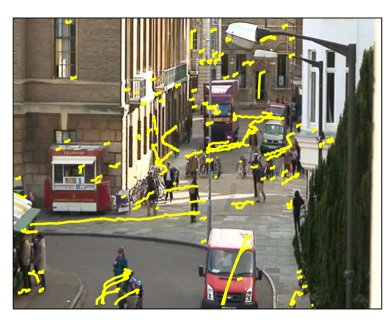
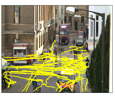
Figure 1: (a) The first 100 feature tracks extracted by our feature tracker. Notice that there are many temporally long tracks with minimal spatial extent due to the apparent motion of stationary features caused by small deflections of the camera by the wind. Filtering using the minimal displacement constraint can be used to reliably detect and discard such tracks. (b) The first 100 feature tracks after filtering.

2.2 Tracklet motion primitives

People’s motion trajectories in a scene can exhibit a wide range variability. However, not all of it is relevant to the problem we address. For example, motion of interest is corrupted by noise and at a short scale modulated by articulation. To reduce the effects of confounding variables on observed motion, we represent all tracks using the same vocabulary of elementary motion primitives, inferred from data, as illustrated conceptually in Figure 2 (a).

2.2.1 Inferring primitives.

We construct the vocabulary of motion primitives by clustering tracklets – local, linear approximations of tracks. We extract a set of tracklets $t_{i}$ from a feature track $T=\left\{(x_{1},y_{1}),\ldots,(x_{N},y_{N})\right\}$ by first dividing the track into overlapping segments $\left\{(x_{s(i)},y_{s(i)}),\ldots,(x_{e(i)},y_{e(i)})\right\}$ such that:

$$\Delta D=\sum_{j=s(i)}^{e(i)-1}\left\|\left(\begin{array}[]{c}x_{j}\\ y_{j}\\ \end{array}\right)-\left(\begin{array}[]{c}x_{j+1}\\ y_{j+1}\\ \end{array}\right)\right\|,$$ (7)

where $\Delta D$ is the characteristic scale parameter of the corresponding tracklet model. The $i$-th tracklet is then defined by a numerical triplet consisting of its location and orientation $t_{i}=(\hat{x}_{i},\hat{y}_{i},\theta_{i})$, where:

$$\hat{x}_{i}=\frac{1}{e(i)-s(i)+1}\sum_{j=s(i)}^{e(i)}x_{j}$$ (8)

$$\hat{y}_{i}=\frac{1}{e(i)-s(i)+1}\sum_{j=s(i)}^{e(i)}y_{j}$$ (9)

$$\hat{\theta}_{i}=\tan^{-1}\frac{y_{e(i)}-y_{s(i)}}{x_{e(i)}-x_{s(i)}}\hskip 10.0pt(\text{mod }\pi)$$ (10)

All tracklets extracted from training data tracks are clustered using an iterative algorithm. In each iteration, a new cluster is initialized with a yet unclustered tracklet as the seed. The cluster is refined further in a nested iteration whereby tracklets are added to the cluster under the constraint of maximal spatial and directional distances, respectively $\Delta Q$ and $\Delta\Theta$, from both the seed and the cluster centre. Cluster centre is then set equal to the mean of the selected tracklets and the procedure repeated until convergence.

Note that the equivalence of directions $\theta$ and $\theta\pm\pi$ introduces some difficulty in the estimation of the cluster centre orientation. Specifically, it is not appropriate to average member directions using modulo $\pi$ arithmetic. First, note that the problem is not always well posed, i.e. that it does not always have a unique solution. Thus, we require that $\forall i.~{}\Delta\hat{\theta}_{i}<\pi/4$, where:

$$\Delta\hat{\theta}_{i}=\min\left\{(\hat{\theta}_{i}-\theta_{c})(\text{mod}~{}\pi),|\hat{\theta}_{i}-\theta_{c}|\right\}.$$ (11)

This condition ensures that the range of directions in a cluster is sufficiently constrained that the mean direction is unambiguously definable. It is sufficient that $\Delta\Theta<\pi/4$ for this to be the case, which is certainly true in this paper, as a directional spread of over $\pi/2$ within a cluster would produce meaningless tracklet groupings. Provided that a unique solution exists, the following pseudo code summarizes the algorithm which correctly updates the cluster centre direction $\theta_{C}$, given a list of directions $\hat{\theta}_{1},\ldots,\hat{\theta}_{N}\in[0,pi)$ of the cluster members:

$\Delta\theta=0$ for $i=1\ldots N$         $\Delta\hat{\theta}_{i}=\hat{\theta}_{i}-\theta_{c}$         if $(\Delta\hat{\theta}_{i}>+\pi/2)$ then $\Delta\hat{\theta}_{i}=\Delta\hat{\theta}_{i}-pi$         if $(\Delta\hat{\theta}_{i}\leq-\pi/2)$ then $\Delta\hat{\theta}_{i}=\Delta\hat{\theta}_{i}+pi$         $\Delta\theta=\Delta\theta+\hat{\theta}_{i}$ end $\theta_{c}=\theta_{c}+\Delta\theta/N$


Figure 2 (b) shows an example of tracklets grouped together and the corresponding cluster centre which becomes a tracklet primitive.

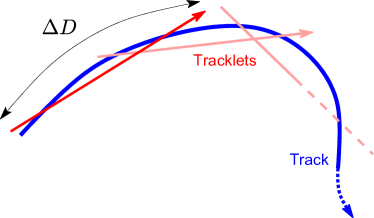
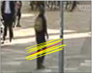
(a)	(b)

Figure 2: (a) By extracting a small set of motion primitives, all tracks can be expressed as sequences of primitives from the same vocabulary. (b) A motion primitive is estimated by clustering fragmented tracks – tracklets – by spatial distance and directional agreement, and computing the mean (location and angle) of each cluster.

2.2.2 Expressing tracks using primitives.

A track is expressed in a particular tracklet model by diving it into overlapping segments, computing the location and direction of each segment as before and, finally, associating each segment $t_{i}=(\hat{x}_{i},\hat{y}_{i},\theta_{i})$ with the most similar tracklet $\mathfrak{T}_{j(i)}=(X_{j(i)},Y_{j(i)},\Theta_{j(i)})$:

$$t_{i}\longrightarrow\mathfrak{T}_{j(i)}:~{}~{}~{}j(i)=\text{arg}\min_{k}\epsilon(\mathfrak{T}_{j},t_{i}),$$ (12)

where:

$$\epsilon(\mathfrak{T}_{j},t_{i})=(X_{j(i)}-\hat{x}_{i})^{2}+(Y_{j(i)}-\hat{y}_{i})^{2}+\left[\frac{\Delta Q}{\tan(\Delta\Theta)}\tan(\Delta\hat{\theta}_{i})\right]^{2}.$$ (13)

This functional form ensures that the angular contribution to distance is infinite for orthogonal tracklets and approximately linear for small $\Delta\hat{\theta}$ (from Taylor’s first order expansion around zero: $\tan\alpha\approx\alpha$), whereas the proportionality factor ensures that relative scaling of spatial and angular distances corresponds to the spread of cluster tracklets.

3 Two tracklet based motion models

In the previous section we described our approach to extraction and representation of motion in a scene. We now turn our attention to the problem of learning a motion model from these low-level representations and applying it to infer novelty in unseen data.

3.1 First order Markov chain ensemble

The first model we introduce in this paper utilizes an ensemble of $K$ complementary first order Markov chains models to learn “normal” behaviour in a scene. The idea is that each model learns behaviour on a different characteristic spatial scale. While this idea is now new, it should be noted that our approach is different in that the ensemble we construct is (in general) not a hierarchial one – states describing behaviour on longer scales do not consist of sequences of lower scale states. Rather, each model is built independently by extracting tracklets and the corresponding motion primitives using different characteristic scales, $\Delta D_{1}<\ldots<\Delta D_{K}$, as proposed in Section 2.2. The $k$-th model thus comprises learnt prior probabilities $P(\mathfrak{T}_{i}^{(k)})$ and transition probabilities $P(\mathfrak{T}_{j}^{(k)}|\mathfrak{T}_{i}^{(k)})$ for tracklet primitives at the corresponding scale.

Consider a particular novel feature track $T=\left\{(x_{1},y_{1}),\ldots,(x_{N},y_{N})\right\}$. In our model, the track is expressed independently in each of the $K$ vocabularies of tracklet primitives:

$$T\longrightarrow\begin{cases}~{}T_{1}=\left\{~{}\mathfrak{T}_{1}^{(1)},~{}\ldots~{},~{}\mathfrak{T}_{M_{1}}^{(1)}~{}\right\}\\ \vspace{-10pt}\\ ~{}T_{2}=\left\{~{}\mathfrak{T}_{1}^{(2)},~{}\ldots~{},~{}\mathfrak{T}_{M_{2}}^{(2)}~{}\right\}\\ ~{}\hskip 35.0pt\vdots\\ ~{}T_{K}=\left\{~{}\mathfrak{T}_{1}^{(K)},~{}\ldots~{},~{}\mathfrak{T}_{M_{k}}^{(K)}~{}\right\}\\ \end{cases}\text{ where \hskip 5.0pt}M_{1}<M_{2}<\ldots M_{K},$$ (14)

where $T_{1}$ corresponds to the smallest scale of interest and $T_{K}$ the largest. Each of the chains can then be used to compute the log-likelihood estimate corresponding to its scale, which we average to normalize for differing track lengths:

$$R_{k}(T)=\frac{1}{M_{k}}\left[\log P(\mathfrak{T}_{1}^{(k)})+\sum_{i=2}^{M_{k}}\log P(~{}\mathfrak{T}_{i}^{(k)}~{}|~{}\mathfrak{T}_{i-1}^{(k)}~{})\right].$$ (15)

Thus, the task of deciding if motion captured by $T$ sufficiently conforms to behaviour seen in training is reduced to inference based on log-likelihoods $R_{1}(T),\linebreak[1]\ldots,\linebreak[1]R_{K}(T)$. This would not be a difficult problem if both positive and negative training data (i.e. both unusual and normal motion patterns) was available, or if log-likelihoods corresponding to different models were directly comparable. However, a representative amount of positive training data is difficult to obtain in this case. Furthermore, although each $R_{i}(T)$ is normalized for track length in (15), the range of variation of its value is dependent on the model’s characteristic scale. This is a consequence of lower entropy (generally) of larger scale models, which have fewer states (tracklet primitives).

To solve this problem, we transform the average log-likelihoods of all models to conform to the same cumulative distribution function of the lowest scale (highest entropy) model:

$$R_{k}\longrightarrow\hat{R}_{k}=\mathcal{C}_{1}^{-1}\left[~{}\mathcal{C}_{k}(R_{k})~{}\right]$$ (16)

where $\mathcal{C}_{k}(R)$ is the cumulative distribution function of the average log-likelihood of the $k$-th Markov chain model, estimated from the training data set:

$$\mathcal{C}_{k}(R)=\int_{-\infty}^{R}p_{k}(r)~{}dr.$$ (17)

We then compute the conformance of the track to the overall multiscale model as the minimal conformance to models over different scales:

$$\rho_{1}(T)=\min_{k}\hat{R}_{k}$$ (18)

3.2 Pursuit-constrained motion model

In the previous section we described an approach to learning the range of normal motion in a scene which treats a feature trajectory as a sequence of states corresponding to extracted tracklet primitives. To make the parameter estimation practically tractable, the sequence of states was modelled as a first order Markov chain which inherently restricts the scope of the model to aggregating single-step behaviour. Progressively less spatially constrained behavioural characteristics were captured by multiple tracklet models, each with a different characteristic scale.

What this approach does not exploit is the structure of observed motion governed by the of intentionality of persons in the scene (whether they are on foot or using a vehicle). While it is certainly the case that if unlimited data was available the described purely statistical model would eventually learn this regularity, this insight can help us achieve a higher degree of generalization from limited data which is available in practice. Our idea is based on the simple observation that people perform motion with the aim of reaching a particular goal and they generally plan their it so as to minimize the invested effort, under the constraints of the scene (such as the locations of boulders and paved areas, or places of interest such as shopping windows). Consequently, we concentrate on learning the distribution of traversed trajectory lengths between two locations in a scene, rather than the exact paths taken between them (a far greater range of possibilities).

Unlike in Section 3.1, we now express a feature track $T$ as a sequence of tracklet primitives only in the vocabulary of the smallest scale of interest:

$$T\longrightarrow T_{1}=\left\{~{}\mathfrak{T}_{1}^{(1)},~{}\ldots~{},~{}\mathfrak{T}_{M_{1}}^{(1)}~{}\right\}.$$ (19)

For each pair of tracklets $\mathfrak{T}_{i}$ and $\mathfrak{T}_{j}$ ($i,j=1,\ldots,M_{1}$) from the sequence we compute the corresponding distance $L_{ij}$ between them along the path. Since the tracklet primitives were estimated using a single scale model with the characteristic scale parameter $\Delta D_{1}$ (see Section 2.2), by construction this distance is given by:

$$L_{ij}=(i-j)~{}\Delta D_{1}/2.$$ (20)

The track is thus decomposed into $M_{1}(M_{1}-1)/2$ triplets $(\mathfrak{T}_{i},\mathfrak{T}_{j},L_{ij})$. We wish to estimate $p(\mathfrak{T}_{i},\mathfrak{T}_{j},L_{ij})$. By expanding the joint probability as:

$$p(\mathfrak{T}_{i},\mathfrak{T}_{j},L_{ij})=P(\mathfrak{T}_{i})~{}~{}P(\mathfrak{T}_{j}~{}|~{}\mathfrak{T}_{i})~{}~{}p(L_{ij}~{}|~{}\mathfrak{T}_{i},\mathfrak{T}_{j}),$$ (21)

we can see that the first two terms – the prior probability of the $i$-th primitive and the probability of $i\rightarrow j$ transition – can be learnt in a similar manner as for the Markov chain based model described previously. On the other hand, the last term corresponding to the distribution of possible path lengths between the $i$-th and $j$-th primitive, is computed by modelling it using a normal distribution:

$$p(\mathfrak{T}_{j}~{}|~{}\mathfrak{T}_{i},L_{ij})=\mathcal{N}(L~{}|~{}\bar{L}_{ij};\sigma_{ij}).$$ (22)

We estimate its parameters – the mean $\bar{L}_{ij}$ and standard deviation $\sigma_{ij}$ – using transitions between primitives observed in the training data set.

Finally, the conformance of a novel track to the learnt motion model is computed as the log of the lowest probability tracklet primitive transition contained within the observed motion:

$$\rho_{2}(T)=\min_{i}\min_{j}\bigg{[}\log p(\mathfrak{T}_{j},\mathfrak{T}_{i},L_{ij})\bigg{]}.$$ (23)

4 Evaluation

Using a stationary camera placed on top of a small building overlooking a busy city marketplace we recorded a video sequence which we used to evaluate the proposed methods. This footage of the total duration of 1h:59m:40s and spatial resolution $720\times 576$ pixels contains all of the challenging aspects used to motivate our work: continuous presence of a large number of moving entities, frequent occlusions, articulation and scale changes, non-static background and large variability in motion patterns. A typical frame is shown in Figure 3 (a) while Figure 3 (b) exemplifies some of the aforementioned difficulties on a magnified subregion.

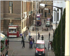
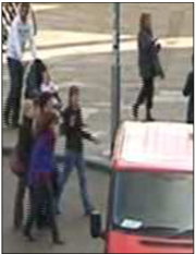
Figure 3: (a) A typical frame extracted from the video footage used in the evaluation of this paper, showing a busy city marketplace, and (b) a magnified image region containing examples of multiple moving objects, mutual occlusion and occlusion by other objects in the scene (car and lamppost), background clutter and shadow patterns which change over time. (c) A synthetic track (green) which our pursuit-constrained motion model based algorithm identifies as unusual, its representation as a sequence of tracklet primitives (yellow) and the pair of primitives (red) corresponding to the most novel behaviour detected in the traversed path.

For the Markov chains ensemble model we used four different characteristic scales, with the corresponding scale parameters $\Delta D_{1}=50,~{}\Delta D_{2}=75,~{}\Delta D_{3}=110,~{}\Delta D_{3}=150$. The lowest scale tracklet model (with $\Delta D_{1}=50$) was used for the pursuit-constrained motion model. The estimation of motion primitives from tracklets was performed using clustering parameters $\Delta Q=25$ and $\Delta\Theta=\pi/16$.

4.1 Results

After training each of the proposed methods using the 113,700 extracted tracks, we computed the corresponding histograms of conformity measures $\rho_{1}$ and $\rho_{2}$. From these we automatically selected thresholds for novelty detection, $R_{1}$ and $R_{2}$, such that 0.05% of training tracks produce lower conformities. An examination of these tracks revealed that the two algorithms generally identified the same tracks as being the least like the rest of the training set with several typical results shown in Figures 5 and 6. A common aspect which can be observed between them is that they correspond to motions which include sharp direction changes at locations in the scene where there is little reason for them. This motion not only novel by the construction of our model but it also conforms to our intuition about what constitutes unusual behaviour. Note the scene-specific, contextual aspect of the learnt motions: many extracted tracks contain sharp turns (e.g. at the end of the row of marketplace stalls or at the corner of the buildings) which are not deemed unusual because the constraints of the scene made such turns (comparatively) frequent in the training data.

Next, to evaluate how our algorithms cope with unseen data, by clicking on the image of the scene we generated a series of synthetic tracks which a human might consider unusual in the context of the marketplace in question. Here, the two methods produced different results. Specifically, consider the examples shown in Figure 4, which the Markov chains ensemble does not classify as novel, unlike the pursuit-constrained motion model. The discrepancy can be explained by observing that in the ensemble approach, a trade-off is made between the precision of motion localization by tracklet primitives and the ability to capture behaviour at a larger scale. Such compromise does not exist in the proposed pursuit-constrained model.

Lastly, since the conformance measure $\rho_{2}$ in (23) is effectively dependent only on a single pair of primitives (those which are explained the worst by the path length model), we visualized these for a series of tracks in which novelty was detected. This is useful as a way of ensuring that the model is capturing meaningful information and potentially in practice as well, by drawing attention not only to a particular behaviour on the whole but a particular feature. This is illustrated with an example in Figure 3 (c) which shows a synthetic track identified as unusual by the pursuit-constrained model, its decomposition into tracklet primitives and the pair of primitives corresponding to the track’s conformance score.

Figure 4: Examples of three synthetic tracks which the Markov chains ensemble model does not classify as novel, and the pursuit-constrained motion model does.

Unusual track 1

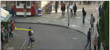
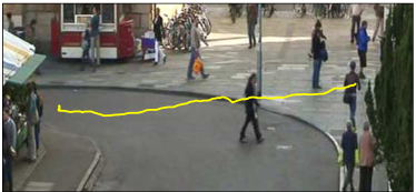
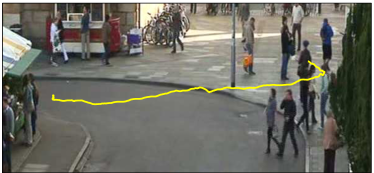
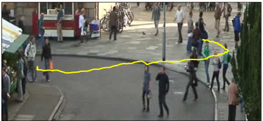
Unusual track 2
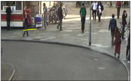
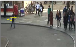
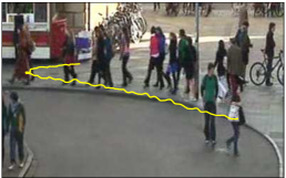
Unusual track 3

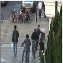
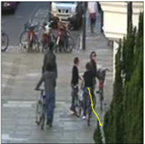
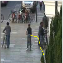
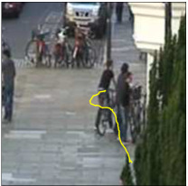
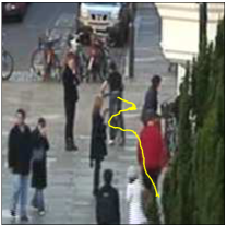
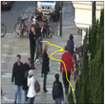
Figure 5: Examples of behaviour detected as unusual by our algorithms. Also see Figure 6.

Unusual track 4

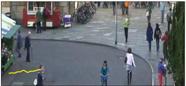
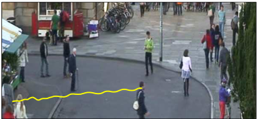
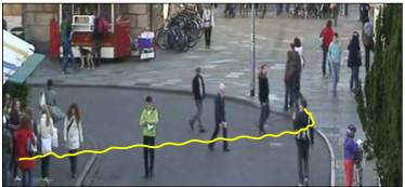
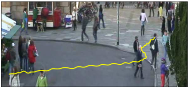
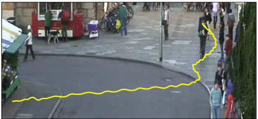
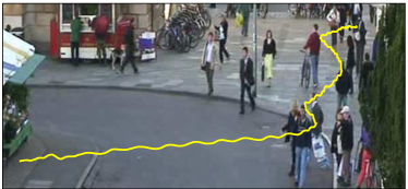
Unusual track 5

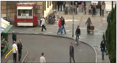
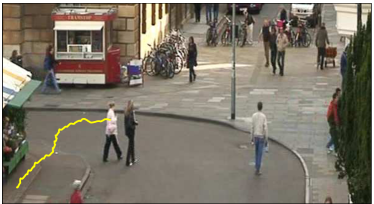
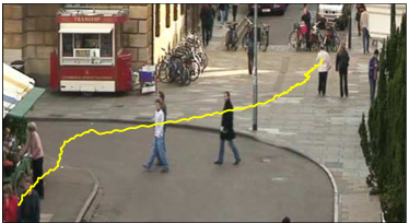
Figure 6: Examples of behaviour detected as unusual by our algorithms. Also see Figure 5.

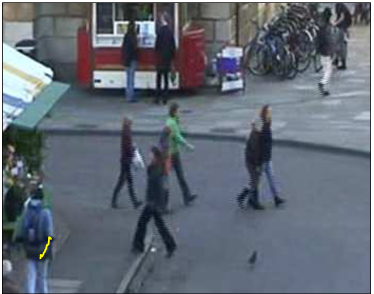
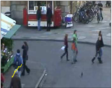
Feature discovery	Successful tracking
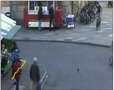
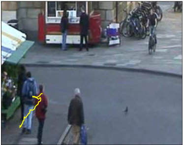
Successful tracking	Incorrect feature matching
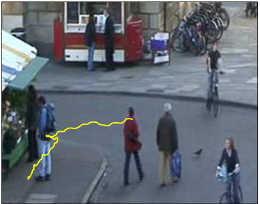
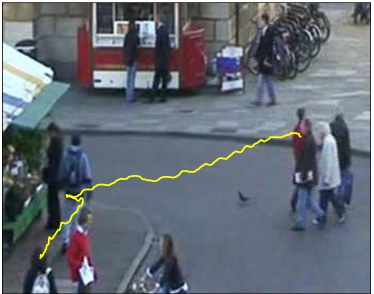
Incorrect feature is tracked	Incorrect feature is tracked

Figure 7: The principal source of errors of our algorithm arises not at the higher level of processing, concerned with how motion is modelled, but rather at the lowest level of motion extraction. Reliable many body tracking in crowded scenes is an outstanding problem.

5 Summary and conclusions

In this paper we addressed the problem of unusual behaviour detection in busy public places by means of novelty detection in holistic body motion. Our general approach is bottom-up. We argued that in the scenario of interest scene motion is best extracted using local features. The obtained feature tracks are segmented into tracklets, which are used to infer scene-specific tracklet primitives using a custom clustering algorithm. Finally, we described two motion models based on tracklet primitives: a multi-scale but non-hierarchial ensemble of Markov chains and an alternative which takes into account human motion planning by learning the distributions of paths lengths between tracklet primitives.

References

- [1] S. Ali and M. Shah. Floor fields for tracking in high density crowd scenes. In Proc. European Conference on Computer Vision (ECCV), II:1–14, 2008.
- [2] O. Arandjelović. Crowd detection from still images. In Proc. IAPR British Machine Vision Conference (BMVC), 1:523–532, September 2008.
- [3] M. Brand and V.M. Kettnaker. Discovery and segmentation of activities in video. IEEE Transactions on Pattern Analysis and Machine Intelligence (TPAMI), 22(8):844–851, 2000.
- [4] G. J. Brostow and R. Cipolla. Unsupervised Bayesian detection of independent motion in crowds. In Proc. IEEE Conference on Computer Vision and Pattern Recognition (CVPR), 1:594–601, 2006.
- [5] A.B. Chan, Z.S.J. Liang, and N. Vasconcelos. Privacy preserving crowd monitoring: Counting people without people models or tracking. In Proc. IEEE Conference on Computer Vision and Pattern Recognition (CVPR), pages 1–7, 2008.
- [6] J.W. Davis and A. Tyagi. Minimal-latency human action recognition using reliable-inference. Image and Vision Computing (IVC), 24(5):455–472, 2006.
- [7] A. Farhadi and M.K. Tabrizi. Learning to recognize activities from the wrong view point. In Proc. European Conference on Computer Vision (ECCV), 1:154–166, 2008.
- [8] W. Hu, X. Xiao, Z. Fu, D. Xie, T. Tan, and S. Maybank. A system for learning statistical motion patterns. IEEE Transactions on Pattern Analysis and Machine Intelligence (TPAMI), 29(9):1618–1626, 2009.
- [9] W. Hu, D. Xie, T. Tan, and S. Maybank. Vector boosting for rotation invariant multi-view face detection. IEEE Transactions on Systems, Man, and Cybernetics – Part B: Cybernetics, 34(3):1618–1626, 2004.
- [10] K.Q. Huang, S. Wang, T.N. Tan, and S.J. Maybank. Multi-frame image restoration and registration. IEEE Transactions on circuits and systems for video technology, 19(12):1830–1840, 2009.
- [11] Y.M. Liang, S.W. Shih, C.C. Shih, H.Y.M. Liao, and C.C. Lin. Learning atomic human actions using variable-length Markov models. IEEE Transactions on Systems, Man, and Cybernetics – Part B: Cybernetics, 39(1):268–280, 2009.
- [12] D. G. Lowe. Distinctive image features from scale-invariant keypoints. International Journal of Computer Vision (IJCV), 60(2):91–110, 2003.
- [13] B.D. Lucas and T. Kanade. An iterative image registration technique with an application to stereo vision. In Proc. International Joint Conference on Artificial Intelligence, I:674–679, 1981.
- [14] N.T. Nguyen, D.Q. Phung, S. Venkatesh, and H.H. Bui. Learning and detecting activities from movement trajectories using the hierarchical hidden Markov models. In Proc. IEEE Conference on Computer Vision and Pattern Recognition (CVPR), 2:955–960, 2005.
- [15] E. Rosten, R. Porter, and T. Drummond. Faster and better: A machine learning approach to corner detection. IEEE Transactions on Pattern Analysis and Machine Intelligence (TPAMI), 2008.
- [16] J. Shi and C. Tomasi. Good features to track. In Proc. IEEE Conference on Computer Vision and Pattern Recognition (CVPR), pages 593–600, 1994.
- [17] D. Tran and A. Sorokin. Human activity recognition with metric learning. In Proc. European Conference on Computer Vision (ECCV), 1:548–561, 2008.
- [18] A. Veeraraghavan, M. Srinivasan, A.K. Roy-Chowdhury, and R. Chellappa. Rate-invariant recognition of humans and their activities. IEEE Transactions on Image Processing, 18(6):1326–1339, 2009.
- [19] A. Yilmaz and M. Shah. A differential geometric approach to representing the human actions. Computer Vision and Image Understanding (CVIU), 109(3):335–351, 2008.
- [20] Z. Zhang, K. Huang, T. Tan, and L. Wang. Trajectory series analysis based event rule induction for visual surveillance. In Proc. IEEE Conference on Computer Vision and Pattern Recognition (CVPR), pages 1–8, 2007.