Excited electronic states from a variational approach based on symmetry-projected Hartree–Fock configurations

Abstract

Recent work from our research group has demonstrated that symmetry-projected Hartree–Fock (HF) methods provide a compact representation of molecular ground state wavefunctions based on a superposition of non-orthogonal Slater determinants. The symmetry-projected ansatz can account for static correlations in a computationally efficient way. Here we present a variational extension of this methodology applicable to excited states of the same symmetry as the ground state. Benchmark calculations on the C₂ dimer with a modest basis set, which allows comparison with full configuration interaction results, indicate that this extension provides a high quality description of the low-lying spectrum for the entire dissociation profile. We apply the same methodology to obtain the full low-lying vertical excitation spectrum of formaldehyde, in good agreement with available theoretical and experimental data, as well as to a challenging model $C_{2v}$ insertion pathway for BeH₂. The variational excited state methodology developed in this work has two remarkable traits: it is fully black-box and will be applicable to fairly large systems thanks to its mean-field computational cost.

I Introduction

The quantum mechanical character of a chemical system is reflected in the discrete spectrum of electronic excitations. From the theoretical point of view, the prediction of geometries and excitation energies provides a means to interpret experimental electronic spectra. In addition, optically forbidden states, which often play an important role in the radiationless relaxation of a molecule, can be accessed.

When the excited state of interest has a different symmetry than the ground state, one can use a ground-state formalism. In the Hartree–Fock (HF) approximation, this approach is usually referred to as the $\Delta$-SCF (self-consistent-field) method. On the other hand, when the excited state of interest has the same symmetry as the ground-state one has to resort to methods explicitly designed to treat excited states.

Quantum chemical methods used to describe excited states can be roughly categorized in two groups Dreuw and Head-Gordon (2005). On the one hand, high-quality wavefunction methods can be used to predict excitation energies and oscillator strengths of low-energy transitions with great accuracy. Among them we find methods based on general multi-configuration SCF (MCSCF) and complete active-space SCF (CASSCF) wavefunctions Werner and Meyer (1981), including the complete active-space second-order perturbation theory (CASPT2) Roos et al. (1996). Equation-of-motion and linear-response coupled-cluster Krylov (2008); Watts (2008), as well as state-universal Li and Paldus (2011) and state-specific Ivanov et al. (2011) multi-reference coupled cluster, approaches can also be used to describe excited state properties. The symmetry-adapted-cluster configuration interaction (SAC CI) Nakatsuji (1979) and Green’s function-based methods Rohlfing (2000) also deserve notice. All these high-quality wavefunction approaches can be used in small systems, although the meaning of “small” has been adapting to the methodological and algorithmic advances seen in recent decades (see, e.g., Ref. Kuś et al., 2009). On the other hand, several prominent methods can be used to access excited states at a reduced computational cost, which permits the description of much larger systems. The time-dependent density functional theory (TD-DFT) Casida and Huix-Rotllant (2012) and configuration-interaction singles (CIS) Foresman et al. (1992) are perhaps the most widely used methods in this category.

In this work, we describe yet another approach to describe excited states of molecular systems by chains of variational calculations based on symmetry-projected configurations. This approach, first proposed by Schmid and co-workers Schmid et al. (1986) has already proved successful in the description of excited states in nuclear systems Schmid (2004). Recently, we have used the same approach to describe ground and excited states of the two-dimensional periodic Hubbard model Rodríguez-Guzmán et al. (2012). In the excited symmetry-projected HF strategy, each state is described by (a set of) symmetry-projected configurations. If the states are of the same symmetry, the orthogonality between the states is enforced by a modification of the ansatz. The advantages of this method are several:

• The method can be regarded as having essentially mean-field computational cost.

• Unlike CIS or TD-DFT, the method can describe two-electron excitations with the same ease as one-electron processes.

• One does not need to compromise between the quality of the ground and excited states as is often done in state-averaged MCSCF approaches.

• Being a wavefunction ansatz, the evaluation of response properties and analytic derivative methods are in principle straightforward.

We show the potential of the method in providing a high-quality low-lying spectrum of molecular systems. In particular, we focus on the dissociation profile of the carbon dimer, which is challenging due to the interaction between two low-lying states of the same symmetry. Additionally, we discuss the application of the method to compute the vertical excitation spectrum of formaldehyde. Due to its simplicity, formaldehyde has been studied using a wide variety of theoretical approaches, which facilitates the comparison with other methods. Lastly, we consider a model of the insertion reaction of Be into H₂, a challenging system commonly used to assess state-of-the-art quantum chemical methods.

This work is organized as follows. In Sec. II we describe in detail the formalism used in terms of symmetry-projected HF configurations. In Sec. III we briefly describe our implementation of the method. We discuss in Sec. IV the application of the method to the description of the dissociation profile of the carbon dimer, the vertical excitation spectrum of formaldehyde, and the insertion reaction of Be into H₂. Sec. V is devoted to concluding remarks.

II Formalism

We present in this section a detailed account of the formalism employed in this work. We begin in Sec. II.1 by describing the symmetry-projected HF ansatz for the ground state of a molecular system with well defined quantum numbers. In Sec. II.2 we set out the excited symmetry-projected HF ansatz for states of the same symmetry as the ground state, an approach introduced by Schmid et al. Schmid et al. (1986). The variational optimization of the considered wavefunctions is discussed in Sec. II.3. Lastly, in Sec. II.4, we describe how one may go about building further correlations in both the ground and excited states Rodríguez-Guzmán et al. (2013), even though this is not something we have carried out in this work.

II.1 Symmetry-projected Hartree–Fock

In a seminal paper, Löwdin Löwdin (1955a) introduced the symmetry-projected HF ansatz for the ground state of a many-body system of fermions. This is expressed as

$$|\Psi\rangle=\hat{P}|\Phi\rangle,$$ (1)

where $\hat{P}$ is a (set of) projection operator(s) that restores the symmetries of a broken symmetry Slater determinant $|\Phi\rangle$. This variational ansatz can account for strong correlations due to spin or orbital degeneracies. It is important to stress that, despite the multi-determinantal character in the wavefunction, the ansatz above does not lose the connection to the single-particle picture: the ansatz is fully determined by the set of molecular orbitals occupied in $|\Phi\rangle$ Löwdin (1966).

In the case of spin projection, Löwdin suggested to use a projection operator of the form

$$\hat{P}^{s}=\prod_{l\neq s}\frac{\hat{S}^{2}-l(l+1)}{s(s+1)-l(l+1)},$$ (2)

where $s$ is used to label the quantum number to be recovered. The projection operator is written as a product of two-body operators rendering it impractical for routine calculations. Following work from the nuclear physics community, we have discussed in Ref. Jiménez-Hoyos et al., 2012a a more convenient form of the projection operators used for spin and point-group symmetry restoration. These are based on the forms introduced by Bayman Bayman (1960) (number) and Villars Villars (1966) (angular momentum). A similar and earlier spin-projection by rotation formalism introduced by Percus and Rotenberg Percus and Rotenberg (1962) has gone largely unnoticed. For spin, we use projection-like operators of the form

$$\hat{P}^{s}_{mk}=\frac{2s+1}{8\pi^{2}}\int d\Omega\,D^{s\ast}_{mk}(\Omega)\,\hat{R}(\Omega),$$ (3)

where $\Omega=(\alpha,\beta,\gamma)$ is the set of Euler angles parametrizing the rotation in spin space, $D^{s}_{mk}(\Omega)\equiv\langle s,m|\hat{R}(\Omega)|s,k\rangle$ is Wigner’s $D$-matrix, and $\hat{R}(\Omega)$ is the spin-rotation operator

$$\hat{R}(\Omega)=\exp\left(-i\alpha\hat{S}_{z}\right)\,\exp\left(-i\beta\hat{S}_{y}\right)\,\exp\left(-i\gamma\hat{S}_{z}\right).$$ (4)

For more details about the form of the projection operators, we refer the reader to Ref. Ring and Schuck, 1980. We note that in Ref. Jiménez-Hoyos et al. (2012a) we incorrectly suggested that if $|\Phi\rangle$ is a UHF-type Slater determinant, the projection operator is simplified. While it is true that matrix elements (norm, Hamiltonian) are simplified (ultimately, a single integration over $\beta$ is required), the projection operator does not change.

In this work, we write the symmetry-projected HF ansatz in the form

$$|\Psi_{j,m}\rangle=\sum_{k}f_{k}\,\hat{P}^{j}_{mk}|\Phi\rangle,$$ (5)

The subscripts $j,m$ in $|\Psi\rangle$ label the irreducible representation and the row of the irrep to recover, respectively . The form above is suitable for arbitrary non-Abelian symmetry groups, including spin. The linear variational coefficients $\{f\}$ are introduced in order to remove unphysical dependencies of the energy with respect to the orientation of the underlying state $|\Phi\rangle$ Schmid et al. (1984); Ring and Schuck (1980).

The energy associated with the symmetry-projected HF state of Eq. 5 is given by

$$E_{j}[\Phi] =\,\frac{\sum_{kk^{\prime}}f_{k}^{\ast}\,f_{k^{\prime}}\,\langle\Phi|\hat{P}_{mk}^{j\dagger}\,\hat{H}\,\hat{P}^{j}_{mk^{\prime}}|\Phi\rangle}{\sum_{kk^{\prime}}f_{k}^{\ast}\,f_{k^{\prime}}\,\langle\Phi|\hat{P}_{mk}^{j\dagger}\,\hat{P}^{j}_{mk^{\prime}}|\Phi\rangle}$$

$$=\,\frac{\sum_{kk^{\prime}}f_{k}^{\ast}\,f_{k^{\prime}}\,\langle\Phi|\hat{H}\,\hat{P}^{j}_{kk^{\prime}}|\Phi\rangle}{\sum_{kk^{\prime}}f_{k}^{\ast}\,f_{k^{\prime}}\,\langle\Phi|\hat{P}^{j}_{kk^{\prime}}|\Phi\rangle},$$ (6)

where we have used the properties of the projection operators Jiménez-Hoyos et al. (2012a) and the fact that they commute with the Hamiltonian. We have emphasized the independence of the energy expression on the row of the irrep selected for non-Abelian groups. We discuss in Appendix A the evaluation of norm and Hamiltonian overlaps between symmetry-projected configurations.

In carrying out the optimization of the wavefunction ansatz of Eq. 5, one can consider two possibilities:

• In a projection-after-variation (PAV) approach, the broken-symmetry mean-field state $|\Phi\rangle$ is optimized variationally. The symmetry-projected energy is then computed in a single-shot evaluation.

• In a variation-after-projection (VAP) approach, the Slater determinant $|\Phi\rangle$ is optimized in the presence of the projection operators.

The PAV approach is appealing for its simplicity. However, it may lead to unphysical behavior: dissociation profiles evaluated with the PAV approach show derivative discontinuities at the point where the broken-symmetry HF solution collapses back to the symmetry-adapted one Schlegel (1986).

The VAP approach is favored not only because it leads to lower energies, but most importantly because the variation is performed for the actual considered ansatz. As it will be shown below, optimizing the state of Eq. 5 in a VAP manner leads to generalized Brillouin-like conditions that characterize the stationary nature of the solution. A self-consistent VAP approach was the basis of the extended Hartree–Fock method proposed by Löwdin Löwdin (1955a). More often than not, EHF has been associated with the use of a spin-projection operator on a reference unrestricted determinant (the so-called spin-projected EHF Mayer (1980)).

Our previous work (Ref. Jiménez-Hoyos et al., 2012a) discussed the self-consistent optimization of the symmetry-projected HF approach. In this work, however, we follow a different strategy to carry out the variational optimization, which we describe in more detail in Sec. II.3.

II.2 The excited symmetry-projected HF approach

Having described the symmetry-projected HF approach for the variational optimization of the ground state of a given symmetry, we now turn our attention to excited states of the same symmetry as the ground state. The excited symmetry-projected HF approach, which relies on a Gram-Schmidt orthogonal construction, was introduced by Schmid et al. Schmid et al. (1986) in the nuclear physics community as the excited VAMP (Variation After Mean-field Projection) strategy.

In order for a given ansatz to constitute a faithful representation of an excited state, it must remain orthogonal to the ground state. In variational strategies, this feature may be accomplished in two alternative ways:

• Use the same ansatz as the one employed in the ground state optimization. The orthogonality with respect to the ground state is enforced as a constraint; that is, one minimizes the Lagrangian

  $$\mathcal{L}[\Psi]=E[\Psi]-\lambda\,\langle\Psi|\Psi_{0}\rangle,$$ (7)

  where $\lambda$ is a Lagrange multiplier and $|\Psi_{0}\rangle$ is the ground state.

• Use an ansatz that is explicitly orthogonal to the ground state wavefunction. This is our preferred approach as the minimization problem remains unconstrained.

Let us assume that the symmetry-projected ground state is already available. This we write as

$$|\Psi^{0}_{j,m}\rangle \equiv\,|\psi^{0}_{j,m}\rangle$$

$$=\,\sum_{k}f^{0}_{k}\,\hat{P}^{j}_{mk}|\Phi^{0}\rangle,$$ (8)

where the $0$ superscript is used to denote the ground state character. Our ansatz for the first excited state is given by

$$|\Psi^{1}_{j,m}\rangle \equiv\,\left(1-\hat{S}^{1}\right)|\psi^{1}_{j,m}\rangle$$

$$=\,\left(1-\hat{S}^{1}\right)\sum_{k}f^{1}_{k}\,\hat{P}^{j}_{mk}|\Phi^{1}\rangle,$$ (9)

written in terms of the projector

$$\hat{S}^{1}=\frac{|\psi^{0}_{j,m}\rangle\,\langle\psi^{0}_{j,m}|}{\langle\psi^{0}_{j,m}|\psi^{0}_{j,m}\rangle},$$ (10)

which guarantees the orthogonality of $|\Psi^{1}_{j,m}\rangle$ with respect to the ground state. Here, the superscript $1$ is used to denote that the first excited state is under consideration. The variational flexibility in the ansatz of Eq. 9 lies in the set of linear variational coefficients $\{f^{1}\}$ and the Slater determinant $|\Phi^{1}\rangle$, which is in general not orthogonal to $|\Phi^{0}\rangle$. Nonetheless, it is important to stress that the actual wavefunction is not a single symmetry-projected configuration but a linear combination.

A similar construction can be used for higher excited states. Having the ground state and $q-1$ excited states already at our disposal, we prepare an ansatz for the $q$-th excited state as

$$|\Psi^{q}_{j,m}\rangle \equiv\,\left(1-\hat{S}^{q}\right)|\psi^{q}_{j,m}\rangle$$

$$=\,\left(1-\hat{S}^{q}\right)\sum_{k}f^{q}_{k}\,\hat{P}^{j}_{mk}|\Phi^{q}\rangle,$$ (11)

with the projector $\hat{S}^{q}$ given by

$$\hat{S}^{q} =\,\sum_{r,s=0}^{q-1}|\psi^{r}_{j,m}\rangle\,\left(A^{-1}\right)_{rs}\,\langle\psi^{s}_{j,m}|,$$ (12)

$$A_{rs} =\,\langle\psi^{r}_{j,m}|\psi^{s}_{j,m}\rangle.$$ (13)

The projector $\hat{S}^{q}$ guarantees orthogonality with respect to the ground state and the $q-1$ excited states previously considered. We note that, along with the linear coefficients $\{f^{q}\}$, a single Slater determinant $|\Phi^{q}\rangle$ determines the full flexibility in the ansatz of Eq. 11. The energy functional associated with the $q$-th excited state wavefunction becomes

$$E^{q}_{j}[\{f^{q}\},|\Phi^{q}\rangle]=\frac{\sum_{kk^{\prime}}f_{k}^{q\ast}\,f_{k^{\prime}}^{q}\,\mathcal{H}^{q}_{kk^{\prime}}}{\sum_{kk^{\prime}}f_{k}^{q\ast}\,f_{k^{\prime}}^{q}\,\mathcal{N}^{q}_{kk^{\prime}}},$$ (14)

where $E^{q}_{j}$ is the energy of the $q$-th excited state. Here, the matrices $\mathcal{N}^{q}$ and $\mathcal{H}^{q}$ are given by

$$\mathcal{N}^{q}_{kk^{\prime}} =\,\langle\Phi^{q}|\hat{P}^{j}_{km}\,\left(1-\hat{S}^{q}\right)\,\hat{P}^{j}_{mk^{\prime}}|\Phi^{q}\rangle,$$ (15a)

$$\mathcal{H}^{q}_{kk^{\prime}} =\,\langle\Phi^{q}|\hat{P}^{j}_{km}\,\left(1-\hat{S}^{q}\right)\,\hat{H}\,\left(1-\hat{S}^{q}\right)\,\hat{P}^{j}_{mk^{\prime}}|\Phi^{q}\rangle.$$ (15b)

We note that even if it may appear otherwise, all matrix elements in the energy functional of Eq. 14 can be evaluated in terms of norm and Hamiltonian overlaps between symmetry-projected configurations (using a single projection operator). For instance,

$$\mathcal{N}^{q}_{kk^{\prime}} =\,\langle\Phi^{q}|\hat{P}^{j}_{km}\,\hat{P}^{j}_{mk^{\prime}}|\Phi^{q}\rangle-\sum_{r,s=0}^{q-1}\sum_{ll^{\prime}}\langle\Phi^{q}|\hat{P}^{j}_{km}\,\hat{P}^{j}_{ml}|\Phi^{r}\rangle\,\left(A^{-1}\right)_{rs}\,\langle\Phi^{s}|\hat{P}^{j}_{l^{\prime}m}\,\hat{P}^{j}_{mk^{\prime}}|\Phi^{q}\rangle\,f_{l}^{r}\,f_{l^{\prime}}^{s\ast}$$

$$=\,\langle\Phi^{q}|\hat{P}^{j}_{kk^{\prime}}|\Phi^{q}\rangle-\sum_{r,s=0}^{q-1}\sum_{ll^{\prime}}\langle\Phi^{q}|\hat{P}^{j}_{kl}|\Phi^{r}\rangle\,\left(A^{-1}\right)_{rs}\,\langle\Phi^{s}|\hat{P}^{j}_{l^{\prime}k^{\prime}}|\Phi^{q}\rangle\,f_{l}^{r}\,f_{l^{\prime}}^{s\ast}.$$

It follows that all states in the irreducible representation $j$ thereby obtained are degenerate. The expressions used to evaluate matrix elements between symmetry-projected configurations are provided in Appendix A. The variational optimization of the energy functional of Eq. 14 is considered in the following subsection.

Let us assume that, through the scheme described above, the ground state and all $q$ excited states have already been obtained. These states, $\{|\Psi^{r}_{j,m}\rangle\,|\,r=0,\ldots,q\}$, are orthogonal among themselves, but they are not necessarily orthogonal through the Hamiltonian. One can therefore carry out a diagonalization of the Hamiltonian in this basis or, equivalently, in the basis of $\{|\psi^{r}_{j,m}\rangle\}$. The eigenvalue equations can be written as

$$B\,g=g\,A\,\varepsilon,$$ (16)

where $g$ is the matrix of eigenvectors, $\varepsilon$ is the diagonal matrix of eigenvalues, $A$ is defined by Eq. 13, and

$$B_{rs}=\langle\psi^{r}_{j,m}|\hat{H}|\psi^{s}_{j,m}\rangle.$$ (17)

In this way, the states $\{|\psi^{r}_{j,m}\rangle\}$ are allowed to interact through the Hamiltonian. The states obtained $\{|\eta^{r}_{j,m}\rangle\,|\,r=0,\ldots,q\}$ through the diagonalization, expressed as

$$|\eta^{r}_{j,m}\rangle =\,\sum_{s=0}^{q}g_{sr}|\psi^{s}_{j,m}\rangle$$

$$=\,\sum_{s=0}^{q}g_{sr}\sum_{k}f^{s}_{k}\,\hat{P}^{j}_{mk}|\Phi^{s}\rangle,$$ (18)

are orthogonal through the Hamiltonian and thus represent a faithful representation of the low-lying spectrum of the considered symmetry. Note also that the final diagonalization of Eq. 16 can account for further correlations in the ground state, that is, beyond those described by the symmetry-projected HF ansatz.

II.3 Variational optimization

We proceed to discuss the strategy we use to variationally optimize wavefunctions based on symmetry-projected configurations. Without loss of generality, we work on the optimization of the $q$-th excited state wavefunction, whose associated energy functional is given by Eq. 14. The ground state optimization can be carried out in a similar fashion. The optimization has to be performed with respect to the set of linear variational coefficients $\{f^{q}\}$ and with respect to the underlying determinant $|\Phi^{q}\rangle$.

The variation of the energy functional (Eq. 14) with respect to $\{f^{q\ast}\}$ leads to the generalized eigenvalue problem

$$\sum_{k^{\prime}}\left(\mathcal{H}^{q}_{kk^{\prime}}-E^{q}_{j}\,\mathcal{N}^{q}_{kk^{\prime}}\right)f^{q}_{k^{\prime}}=0\qquad\forall\qquad k,$$ (19)

which has to be solved subject to the normalization constraint

$$f^{q\dagger}\,\mathcal{N}^{q}\,f^{q}=\mathbf{1}_{d^{\prime}},$$ (20)

where $d^{\prime}\leq d$ and $d$ is the dimension of the irreducible representation recovered by the projection. The Hamiltonian $\mathcal{H}^{q}$ and overlap $\mathcal{N}^{q}$ matrices are given by Eqs. 15b and 15a, respectively. In addition, $E^{q}_{j}$ is the lowest-energy solution to the eigenvalue problem (it constitutes the energy of the $q$-th excited state); all other solutions are discarded at this point.

The variation of the energy functional with respect to the underlying determinant, $|\Phi^{q}\rangle$, is more convoluted. We use a parametrization based on the Thouless theorem, which states that the $N$-electron Slater determinant $|\Phi^{q}\rangle$ can be written in terms of another (reference) $N$-electron Slater determinant $|\Phi\rangle$ as

$$|\Phi^{q}\rangle =\,\eta\,\exp(\hat{Z}^{q})|\Phi\rangle,$$ (21)

$$\hat{Z}^{q} =\,\sum_{ph}Z^{q}_{ph}\,b_{p}^{\dagger}\,b_{h},$$ (22)

as long as $|\Phi^{q}\rangle$ is not orthogonal to $|\Phi\rangle$. Here, $\eta=\langle\Phi^{q}|\Phi\rangle$ is a normalization factor, and the sum in Eq. 22 is over particle and hole operators defined by the orbitals characterizing $|\Phi\rangle$. The coefficients $Z^{q}_{ph}$ are unique.

The Thouless theorem permits an efficient parametrization of the Slater determinant $|\Phi^{q}\rangle$. That is, we use Eq. 21 and treat the coefficients $Z^{q}_{ph}$ as variational parameters. We note that this Thouless parametrization has not been frequently used in chemistry. Mang Mang (1975), among others, suggested its use in the nuclear physics community in the context of a Hartree–Fock–Bogoliubov reference vacuum. Recently, Noga and Šimunek Noga and Šimunek (2010) used a Thouless matrix, in a unitary coupled-cluster singles framework, to carry out the optimization of independent particle model wavefunctions. Their approach is similar in spirit to ours, though the actual algorithm has important differences. A Thouless-based optimization is also closely related to the quadratically-convergent algorithm suggested by Backsay Backsay (1981). We point the interested reader to Refs. Egido et al., 1995; Jiménez-Hoyos, 2013 for a more detailed description of the approach we use.

Using Eq. 21, we can write the energy functional of Eq. 14 as one depending on the coefficients $Z^{q}_{ph}$,

$$E^{q}_{j}[\{f^{q}\},Z^{q}]=\frac{\displaystyle\sum_{kk^{\prime}}f_{k}^{\ast q}\,f_{k^{\prime}}^{q}\,\langle\Phi|\exp(\hat{Z}^{q\dagger})\,\hat{P}^{j}_{km}\,\left(1-\hat{S}^{q}\right)\,\hat{H}\,\left(1-\hat{S}^{q}\right)\,\hat{P}^{j}_{mk^{\prime}}\exp(\hat{Z}^{q})|\Phi\rangle}{\displaystyle\sum_{kk^{\prime}}f_{k}^{\ast q}\,f_{k^{\prime}}^{q}\,\langle\Phi|\exp(\hat{Z}^{q\dagger})\,\hat{P}^{j}_{km}\,\left(1-\hat{S}^{q}\right)\,\hat{P}^{j}_{mk^{\prime}}\exp(\hat{Z}^{q})|\Phi\rangle},$$ (23)

where $|\Phi\rangle$ is an arbitrary reference state used for the minimization.

A stationary point of the energy functional of Eq. 23 is reached when the energy gradient, given by

$$G^{q}_{ph} \equiv\,\frac{\partial}{\partial Z^{q\ast}_{ph}}\,E^{q}_{j}[\{f^{q}\},Z^{q}]$$

$$=\,\frac{\displaystyle\sum_{kk^{\prime}}f_{k}^{\ast q}\,f_{k^{\prime}}^{q}\,\langle\Phi^{q}|b_{h}^{\dagger}\,b_{p}\,\hat{P}^{j}_{km}\,\left(1-\hat{S}^{q}\right)\,\left(\hat{H}-E^{q}_{j}\right)\left(1-\hat{S}^{q}\right)\,\hat{P}^{j}_{mk^{\prime}}|\Phi^{q}\rangle}{\displaystyle\sum_{kk^{\prime}}f_{k}^{\ast q}\,f_{k^{\prime}}^{q}\,\langle\Phi^{q}|\hat{P}^{j}_{km}\,\left(1-\hat{S}^{q}\right)\,\hat{P}^{j}_{mk^{\prime}}|\Phi^{q}\rangle},$$ (24)

vanishes for all elements of $G^{q}$. Here, the HF operators $b_{h}^{\dagger}$ and $b_{p}$ are associated with the determinant $|\Phi\rangle$ (and not $|\Phi^{q}\rangle$). This is sometimes referred to as the global gradient. The local gradient $\mathcal{G}^{q}$ at $|\Phi\rangle=|\Phi^{q}\rangle$, given by

$$\mathcal{G}^{q}_{ph} \equiv\,\left.\frac{\partial}{\partial Z^{q\ast}_{ph}}\,E^{q}_{j}[\{f^{q}\},Z^{q}]\right|_{Z^{q}_{ph}=0}$$

$$=\,\frac{\displaystyle\sum_{kk^{\prime}}f_{k}^{\ast q}\,f_{k^{\prime}}^{q}\,\langle\Phi^{q}|b_{h}^{q\dagger}\,b_{p}^{q}\,\hat{P}^{j}_{km}\,\left(1-\hat{S}^{q}\right)\,\left(\hat{H}-E^{q}_{j}\right)\left(1-\hat{S}^{q}\right)\,\hat{P}^{j}_{mk^{\prime}}|\Phi^{q}\rangle}{\displaystyle\sum_{kk^{\prime}}f_{k}^{\ast q}\,f_{k^{\prime}}^{q}\,\langle\Phi^{q}|\hat{P}^{j}_{km}\,\left(1-\hat{S}^{q}\right)\,\hat{P}^{j}_{mk^{\prime}}|\Phi^{q}\rangle},$$ (25)

in which HF operators associated with $|\Phi^{q}\rangle$ are used, can be related to the global gradient by Jiménez-Hoyos et al. (2012b)

$$G^{q}=\tilde{L}^{\mathsf{T}-1}\,\mathcal{G}^{q}\,L^{\ast-1}.$$ (26)

Here, $\tilde{L}$ and $L$ are $(M-N)\times(M-N)$ and $N\times N$ matrices, respectively, obtained from standard Cholesky decompositions (see Ref. Jiménez-Hoyos et al., 2012b). We note that the local gradient also vanishes at a stationary point of the energy functional.

Once the optimal $|\Phi^{q}\rangle$ has been found, it is convenient to have a unique representation of the molecular orbitals characterizing the Slater determinant (recall that the functional is invariant to unitary transformations among the occupied orbitals). This can be accomplished by diagonalizing the $H^{11}$ sector of the Hamiltonian, whose hole-hole and particle-particle blocks are given by

$$H^{11}_{hh^{\prime}}=\langle\Phi^{q}|b_{h}^{\dagger}\,H\,b_{h^{\prime}}^{\dagger}|\Phi^{q}\rangle-\delta_{hh^{\prime}}\langle\Phi^{q}|\hat{H}|\Phi^{q}\rangle,$$ (27a)

$$H^{11}_{pp^{\prime}}=\langle\Phi^{q}|b_{p}\,H\,b_{p^{\prime}}^{\dagger}|\Phi^{q}\rangle-\delta_{pp^{\prime}}\langle\Phi^{q}|\hat{H}|\Phi^{q}\rangle.$$ (27b)

Note that this is simply a way of finding semi-canonical orbitals, using traditional quantum chemical jargon.

We close this section by listing some of the advantageous features that a variational optimization based on a Thouless parametrization provides:

• The minimization problem is unconstrained, with as many parameters as linearly independent variables. Powerful algorithms (conjugate gradient, quasi-Newton methods) for unconstrained minimization can be used Nocedal and Wright (2006).

• Because of the gradient-based approach used, one is guaranteed that the optimization will either converge to a stationary point within a specified tolerance or the algorithm used will fail.

• The application of the method to symmetry-projected approaches or arbitrary wavefunctions expressed in terms of Slater determinants is straightforward.

• The method does not require one to a priori decide how to occupy the orbitals, which a diagonalization approach requires. For HF, an aufbau occupation leads to the lowest energy solution, but the same need not be true for more general functionals.

II.4 Correlations in the ground and excited states

In the previous sections, we have considered an ansatz for the ground and excited states of a given symmetry. Each state is described by essentially a single symmetry-projected HF configuration. If this description proves insufficient, one can consider a more general ansatz written as a linear combination of symmetry-projected configurations as a trial wavefunction for each state. This approach has been used to describe ground-state correlations of molecular systems in Ref. Jiménez-Hoyos et al., 2013 and in the Hubbard model in Ref. Rodríguez-Guzmán et al., 2013. We briefly describe the idea in this section, even though we do not include results from such multi-component approach in our calculations.

In a multi-component approach, the ground state is expanded as a linear combination of symmetry-projected configurations

$$|\Psi^{0}_{j,m}\rangle \equiv\,|\psi^{0}_{j,m}\rangle$$

$$=\,\sum_{k}\hat{P}^{j}_{mk}\sum_{z=1}^{n_{0}}f^{0}_{z;k}|\Phi^{0}_{z}\rangle.$$ (28)

Here, once again the superscript $0$ denotes the ground state character of the considered ansatz. The trial wavefunction is expanded as a linear combination of $n_{0}$ symmetry-projected configurations, obtained from the corresponding set of (non-orthogonal) Slater determinants $\{|\Phi^{0}_{z}\rangle\,|\,z=1,\ldots,n_{0}\}$.

The ansatz for the $q$-th excited state is similar to that from the single-configuration approach. It is given by

$$|\Psi^{q}_{j,m}\rangle \equiv\,\left(1-\hat{S}^{q}\right)|\psi^{q}_{j,m}\rangle$$

$$=\,\left(1-\hat{S}^{q}\right)\sum_{k}\hat{P}^{j}_{mk}\sum_{z=1}^{n_{q}}f^{q}_{z;k}|\Phi^{q}_{z}\rangle,$$ (29)

with the projector $\hat{S}^{q}$ given by an expression analogous to Eq. 12. (Note, nonetheless, that each state $|\psi^{r}_{j,m}\rangle$ is given by a linear combination of $n_{r}$ symmetry-projected configurations.)

One may now wonder how the variational optimization is performed in this multi-component approach. The two extreme strategies are:

• All the determinants $\{|\Phi^{q}_{z}\rangle\,|\,z=1,\ldots,n_{q}\}$ describing the $q$-th excited state are optimized at once. This is known in the literature as the resonating Hartree–Fock approach (Res HF), first introduced by Fukutome Fukutome (1988).

• A step-wise construction is used in which only the last added determinant is optimized while the previously obtained remain frozen. This is known, in the nuclear physics community, as the few-determinant (FED) approach introduced by Schmid et al. Schmid et al. (1989). In combination with the Gram-Schmidt orthogonal construction used for the excited states, it is referred to as the excited FED VAMP strategy Schmid et al. (1989). We note that a similar approach, even if Slater determinants were used in place of the symmetry-projected configurations, was employed by Koch and Dalgaard Koch and Dalgaard (1993) in ground state optimizations.

We refer the reader to our recent work on the one-dimensional Hubbard Hamiltonian Rodríguez-Guzmán et al. (2013) where the merits of this approach have been discussed.

III Computational details

We have developed a computer program that can optimize symmetry-projected HF states (as well as excited states) using a Thouless parametrization, as described in Sec. II.3. This is different from our original work (see Ref. Jiménez-Hoyos et al., 2012a), which used a diagonalization based approach. A limited-memory Broyden–Fletcher–Goldfarb–Shanno (BFGS) Nocedal (1980); Liu and Nocedal (1989) quasi-Newton method is used as the unconstrained minimization algorithm. The program interfaces with the GAUSSIAN suite Frisch et al. to retrieve one- and two-electron integrals. Our program is parallelized (MPI-based) over the grid to perform the symmetry restoration (spatial and/or spin). We note that if a single symmetry-projected configuration is used to describe each state (as done in this work), the excited method scales linearly with the order of the state described. That is, the optimization of the first excited state is twice as expensive as that of the ground state. Unfortunately, we have not yet implemented the capability of evaluating oscillator strengths of the excited states, but it is straightforward to do so once the appropriate integrals are available. We prepare an initial guess for the broken symmetry determinants by taking the converged HF solution and mixing a few orbitals closest to the Fermi energy using a randomly prepared unitary matrix. A similar strategy has been used in our recent study of the one-dimensional Hubbard model Rodríguez-Guzmán et al. (2013).

IV Results and discussion

We discuss the application of the excited symmetry-projected HF method to three different systems: the dissociation profile of the carbon dimer, the vertical excitation spectrum of formaldehyde, and a model for the insertion reaction of Be in H₂. We consider simple systems in small basis in order to compare with previously reported results. Lastly, we emphasize that, in order to showcase the excited symmetry-projected HF strategy, it has to be applied to systems for which a few excited states of the same symmetry are of interest.

IV.1 Dissociation profile of the carbon dimer

We consider the dissociation profile of the carbon dimer in the 6-31G(d) basis, for which the full CI (FCI) dissociation profile was reported by Abrams and Sherrill in Ref. Abrams and Sherrill (2004). The correct description of the dissociation profile of the carbon dimer is quite challenging from a theoretical point of view: not only is a double-bond being broken, but there is a low-lying excited state of the same-symmetry (${}^{1}\Sigma_{g}^{+}$) as the ground state nearby in energy. In fact, an avoided crossing occurs at $\approx 1.7\,\mathring{\mathrm{A}}$, where the character of the two states is interchanged. In addition, there is also a low-lying ${}^{1}\Delta_{g}$ state that becomes the ground state at large interatomic separation. A further complication arises because, as described by Abrams and Sherrill, within the $D_{2h}$ subgroup available in most quantum chemical packages, the ${}^{1}\Sigma_{g}^{+}$ and the ${}^{1}\Delta_{g}$ states have the same ${}^{1}A_{g}$ symmetry Abrams and Sherrill (2004).

An assessment of the ability of several sophisticated quantum chemical methods to describe the dissociation profile was presented in Refs. Abrams and Sherrill (2004) and Sherrill and Piecuch (2005). Most coupled-cluster approaches fail to provide even a qualitatively correct description of the dissociation profile of the ground state, with its characteristic non-Morse-like behavior due to the avoided crossing. Only multi-reference approaches such as CASPT2 or multi-reference CI Sherrill and Piecuch (2005) can accurately describe the dissociation profile of all three states considered.

The dissociation profile of four low-lying singlet states of C₂ as predicted with the excited $D_{4h}$S-UHF method is shown in Fig. 1. Here, the $D_{4h}$S-UHF notation implies that spin projection (S) and spatial symmetry-restoration (in the $D_{4h}$ point group) have been broken and restored from an underlying determinant of unrestricted HF (UHF) character. The use of the $D_{4h}$ subgroup allows us to distinguish between the ${}^{1}\Sigma_{g}^{+}$ and the ${}^{1}\Delta_{g}$ irreducible representations of the $D_{\infty h}$ group: the ${}^{1}\Delta_{g}$ state transforms as the ${}^{1}B_{1g}$ irreducible representation in the $D_{4h}$ subgroup. For the two ${}^{1}A_{1g}$ states we show the profiles obtained before (top panel) and after (bottom panel) they are allowed to interact through the Hamiltonian in the final diagonalization of Eq. 16.

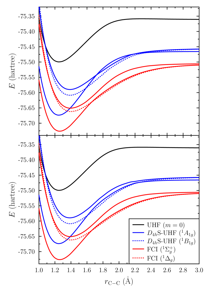
Figure 1: Dissociation profiles for low-lying singlet states of the C₂ molecule computed with the $D_{4h}$S-UHF / 6-31G(d) method. A comparison with FCI curves from Ref. Abrams and Sherrill (2004) is shown. The $D_{4h}$S-UHF profiles for the two ${}^{1}A_{1g}$ states as obtained before (top panel) and after (bottom panel) the final diagonalization (Eq. 16) are displayed. The avoided crossing is correctly described after the two ${}^{1}A_{1g}$ states are allowed to interact through the Hamiltonian.

Several features of the exact dissociation profile are correctly described with our $D_{4h}$S-UHF approximation. In particular, we observe that the $B_{1g}$ state is correctly predicted to be the lowest energy state for $r_{\mathrm{C-C}}>1.6\,\mathring{\mathrm{A}}$. The avoided crossing observed in the FCI profile appears after the two ${}^{1}A_{1g}$ symmetry-projected configurations are allowed to interact. In this way, the dissociation profile predicted for the lowest-lying ${}^{1}A_{1g}$ state correctly displays the characteristic non-Morse-like behavior. One should note, however, that the carbon-carbon distance of closest approach between the two ${}^{1}A_{1g}$ states is slightly larger than in the FCI solution. We finally point out that the curves obtained for the three states for which the FCI solution is available are fairly parallel to the latter. This validates our description of the ground and excited states of C₂ in terms of symmetry-projected configurations. We emphasize that essentially a single symmetry-projected configuration was used for each state: two symmetry-projected configurations were used to describe two states of ${}^{1}A_{1g}$ symmetry.

IV.2 Vertical excitation spectrum of formaldehyde

Formaldehyde is the simplest of the carbonyl compounds and as such it is ubiquitous in nature. The presence of a $\pi$-electron system and the lone pairs of oxygen permit $n\rightarrow\pi^{\ast}$ and $\pi\rightarrow\pi^{\ast}$ valence transitions, making formaldehyde photochemically active. Because of its small size and availability, formaldehyde has been widely studied both experimentally and theoretically.

Some vertical excitation transitions of formaldehyde have been experimentally determined (see Refs Robin (1985) and Taylor et al. (1982)). The vertical excitation spectrum of formaldehyde has been studied theoretically by several authors, both to help in the assignment of the spectrum, as well as to test different theoretical approaches. We refer the reader to the work by Hadad et al. Hadad et al. (1993), Pitarch-Ruiz et al. Pitarch-Ruiz et al. (2003), and references therein. Recently, Schreiber et al. Schreiber et al. (2008) have provided best theoretical estimates for some low-energy valence and Rydberg transitions of formaldehyde.

Our focus here is to test whether our approach can provide reasonable excitation energies. In particular, we focus on the vertical excitation spectrum as we currently lack the ability to optimize the geometries of ground and excited states. We use the ground state $C_{2v}$ geometry from Ref. Hadad et al. (1993) (optimized with MP2/6-31G(d)). The basis set 6-311(2+,2+)G(d,p) we use was also obtained from the same work. The second set of diffuse functions was found necessary in order to correctly describe the Rydberg transitions at the CIS level.

In Fig. 2 we show how six different singlet $A_{1}$ states are obtained by the chain of variational calculations defined in the excited symmetry-projected ($C_{2v}$S-UHF) approach. Here, the notation $C_{2v}$S-UHF implies that spin and spatial symmetry (in the $C_{2v}$ framework) is restored from a broken symmetry UHF-type determinant. Observe that the states are not necessarily obtained in a strict increasing-energy order. In our $C_{2v}$S-UHF calculations for triplet states, we have used an $m_{s}=1$ UHF-type determinant; the use of $m_{s}=0$ determinants would lead to different results . The right-most column shows the resulting set of states after the final diagonalization of Eq. 16. In this particular case, the ground state gains almost no additional correlations as it is well separated from other states energetically. On the other hand, several of the states interact strongly as evidenced by the large differences observed from column 6 to the column labeled as “final”.

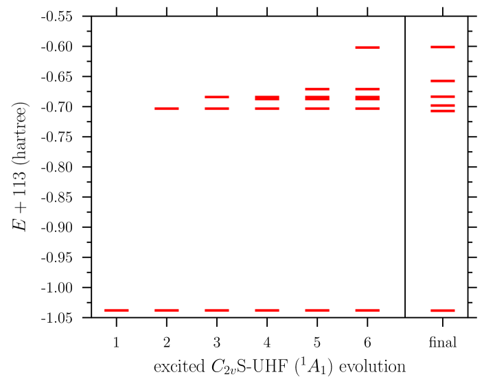
Figure 2: Evolution of the ${}^{1}A_{1}$ spectrum of formaldehyde as computed with the excited $C_{2v}$S-UHF method with increasing number of symmetry-projected configurations. The last column shows the spectrum obtained after the final diagonalization of Eq. 16 is carried out.

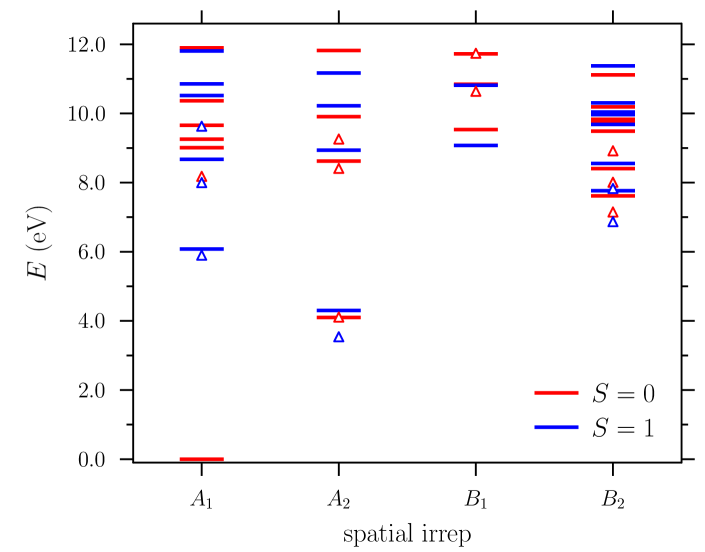
Figure 3: Low-lying singlet and triplet states of the formaldehyde molecule predicted with the $C_{2v}$S-UHF method. The 6-311(2+,2+)G(d,p) basis was used in the calculations. Experimental excitation energies from Refs. Robin, 1985; Taylor et al., 1982; Hadad et al., 1993 are shown as red and blue triangles for singlet and triplet states, respectively.

We show, in Fig. 3 the full low-lying singlet and triplet vertical spectrum of formaldehyde predicted with the $C_{2v}$S-UHF approach. A comparison with experimental results from Refs. Robin, 1985; Taylor et al., 1982 and a few other results compiled in Ref. Hadad et al., 1993 is also provided. As we have used a limited basis set and our treatment of electron correlation is only approximate, we cannot expect perfect agreement with experimental numbers. The agreement between our $C_{2v}$S-UHF and the experimental excitation energies (for both singlet and triplet states) is remarkable, as each of the states obtained is described by essentially a single symmetry-projected configuration. There is no a priori reason to expect that all states should be well approximated by a single symmetry-projected configuration, or that the quality obtained for the different irreducible representations should be comparable. Nevertheless, the agreement with the experimental excitation energies is quite good, with maximum deviations of $\approx 1$ eV for both singlet and triplet states.

We show in Table 1 a comparison of the predicted low-lying vertical excitation of formaldehyde with $C_{2v}$S-UHF and other results available from the literature. In particular, we compare with the CIS and CIS-MP2 results of Ref. Hadad et al. (1993), where the latter includes an electron correlation correction to the CIS energies via perturbation theory through second order, and with the (SC)² multi-reference (MR) CI with singles and doubles (SD) of Ref. Pitarch-Ruiz et al. (2003), which constitute best available theoretical estimates. The (SC)² scheme is a self-consistent dressing procedure that, among other effects, corrects the size-extensivity of MR-CI Daudey et al. (1993). The CIS and CIS-MP2 calculations use the same basis set and geometry that we have used. The MR-CISD calculations use a large atomic natural-orbital-type [$6s5p3d2f/4s3p2d$] basis for C,O/H augmented with a $3s3p3d$ adapted Rydberg series. The latter diffuse functions were placed in the charge center of the ${}^{2}B_{2}$ state of the formaldehyde cation. The ground-state geometry used in MR-CISD calculations was described in Ref. Pitarch-Ruiz et al., 2003; it deviates $\approx 0.01\mathring{\mathrm{A}}$ in bond-lengths and $\approx 1^{\circ}$ in the H-C-H angle with respect to the MP2/6-31G(d) optimized geometry. The states in Table 1 are ordered according to:

• The CIS and CIS-MP2 states are listed in increasing order according to the CIS-MP2 excitation energies.

• Experimental vertical excitations are listed according to the assignment provided in Ref. Hadad et al., 1993 with respect to CIS results.

• MR-CISD results are listed in increasing order, trying to match the assignments provided in Ref. Pitarch-Ruiz et al., 2003 with those in Ref. Hadad et al., 1993.

• The $C_{2v}$S-UHF excitation energies are listed in increasing order as we have not tried to make a formal assignment of the excitation energies. Such an assignment would only provide a guide for interpretation as states of the same symmetry always possess mixed character.

Table 1: Vertical excitation energies (in eV) of formaldehyde as predicted by the excited $C_{2v}$S-UHF, CIS, CIS-MP2, and (SC)²-MR-CISD methods compared to the available experimental data. The states are listed according to their spin and spatial-symmetry labels. (See text for a description of the ordering used in listing the states.)

	singlets						triplets
label	EPHF	CIS	CIS-MP2	MRCI	expt		EPHF	CIS	CIS-MP2	MRCI	expt
$A_{1}$	$9.01$	$9.66$	$8.47$	$8.27$	$8.14$		$6.08$	$4.65$	$6.72$	$6.05$	$5.86$
	$9.25$	$10.88$	$8.75$	$9.31$			$8.67$	$9.31$	$7.78$	$8.15$	$7.96$
	$9.66$	$9.45$	$9.19$	$9.68$			$10.52$	$10.56$	$9.12$	$9.35$	$9.59$
	$10.37$	$11.24$	$9.20$				$10.85$	$10.88$		$9.64$
	$11.90$	$12.09$	$9.99$				$11.81$	$11.89$
$A_{2}$	$4.10$	$4.48$	$4.58$	$4.04$	$4.07$		$4.30$	$3.67$	$4.15$	$3.59$	$3.50$
	$8.62$	$9.78$	$7.83$	$8.36$	$8.37$		$8.94$	$9.72$	$8.16$	$8.41$
	$9.91$	$10.92$	$10.08$	$9.34$	$9.22$		$10.22$	$10.20$	$10.52$	$9.37$
	$11.82$	$12.06$	$10.13$				$11.17$	$11.15$
		$11.37$	$10.49$
		$11.93$	$11.63$
$B_{1}$	$9.53$	$9.66$	$9.97$	$9.33$			$9.07$	$8.37$	$9.18$	$8.52$
	$10.84$	$11.05$	$10.84$		$10.60$		$10.82$	$10.86$		$9.33$
	$11.72$	$11.84$	$11.56$		$11.70$		$13.75$	$11.56$
$B_{2}$	$7.62$	$8.63$	$6.85$	$7.12$	$7.11$		$7.76$	$8.28$	$6.97$	$6.98$	$6.83$
	$8.40$	$9.36$	$7.66$	$7.95$	$7.97$		$8.55$	$9.04$	$7.75$	$7.81$	$7.79$
	$9.49$	$10.61$	$8.46$	$8.96$	$8.88$		$9.68$	$10.33$	$8.67$	$8.83$
	$9.77$	$10.86$	$8.94$	$9.18$			$9.97$	$10.69$		$9.16$
	$9.83$	$10.98$	$8.96$	$9.27$			$10.04$	$10.80$
	$10.19$	$11.17$	$9.19$				$10.30$	$11.07$
	$11.11$						$11.38$

The results shown in Table 1 show a surprisingly good qualitative agreement between our $C_{2v}$S-UHF calculations and the MR-CISD and experimental vertical excitation energies. In particular, the $C_{2v}$S-UHF results significantly improve over CIS for most of the excitations listed in the table. Larger deviations are observed for states with significant Rydberg character, suggesting that the basis set used is still not sufficient to converge such excitation energies. The observed agreement between $C_{2v}$S-UHF excitation energies with best theoretical estimates is encouraging as it showcases the ability of the simple, mean-field excited symmetry-projected HF approach to describe excited states of molecular systems.

IV.3 $C_{2v}$ insertion pathway for BeH₂

The model $C_{2v}$ insertion pathway of Be into H₂ is a known challenging system. It was originally proposed by Purvis et al. Purvis, III et al. (1983) as testing ground for single-reference coupled-cluster methods. It has recently been used as a benchmarking case for novel multi-reference based methods (see Ref. Evangelista et al., 2006 and references therein).

We follow Ref. Evangelista et al., 2006 in the construction of the model pathway: with the beryllium atom placed at the origin, the $y$ coordinates (in bohr) of the hydrogen atoms are related to their $x$ coordinates (in bohr) by the equation

$$y(x)=\pm(2.54-0.46x)\qquad x\in[0,4].$$

At $x=0$, the geometry described corresponds approximately to the BeH₂ equilibrium geometry, while at $x=4$, the geometry corresponds to a hydrogen molecule at equilibrium interacting with a Be atom placed $4$ bohr away. A linear interpolation is used for intermediate geometries; the model insertion pathway has $C_{2v}$ symmetry. In our calculations, we use the same small basis set as that used in Ref. Evangelista et al., 2006, corresponding to the contraction scheme Be($10s3p/3s2p$) and H($4s/2s$).

The BeH₂ model insertion pathway is challenging as the dominant configurations in the FCI expansion change character. At the equilibrium BeH₂ geometry, the dominant configuration is

$$(1\sigma_{g})^{2}\,(2\sigma_{g})^{2}\,(1\sigma_{u})^{2}\qquad\equiv\qquad(1a_{1})^{2}\,(2a_{1})^{2}\,(1b_{2})^{2},$$

where the l.h.s. configuration uses the $D_{\infty h}$ symmetry of the linear molecule and the r.h.s. is its representation in the $C_{2v}$ subgroup. On the other hand, at dissociation, the dominant configuration becomes

$$(1a_{1})^{2}\,(2a_{1})^{2}\,(3a_{1})^{2}.$$

Note hat the latter corresponds to a double excitation with respect to the reference determinant near the BeH₂ equilibrium. Excited state methods based on a particle-hole construction out of a symmetry-adapted reference would therefore fail to provide even a qualitatively correct profile for the first excited state. Single-reference coupled-cluster can correctly describe the ground-state dissociation pathway only when different references are used in different intervals of $x$ Purvis, III et al. (1983); Evangelista et al. (2006); the resulting curve is, nevertheless, discontinuous. We note that different flavors of multi-reference coupled-cluster can correctly describe the model insertion pathway Evangelista et al. (2006).

We show in Fig. 4 the insertion pathways predicted by UHF, $C_{2v}$S-UHF, and $C_{2v}$KS-UHF, as a function of the $x$ coordinate of the hydrogen atoms. In $C_{2v}$S-UHF, the full-spin symmetry and the spatial symmetry ($C_{2v}$) are broken and restored self-consistently; in $C_{2v}$KS-UHF, we additionally break and restore complex conjugation (denoted by K). We also present the ground state FCI curve (obtained from Ref. Evangelista et al., 2006) for comparison purposes.

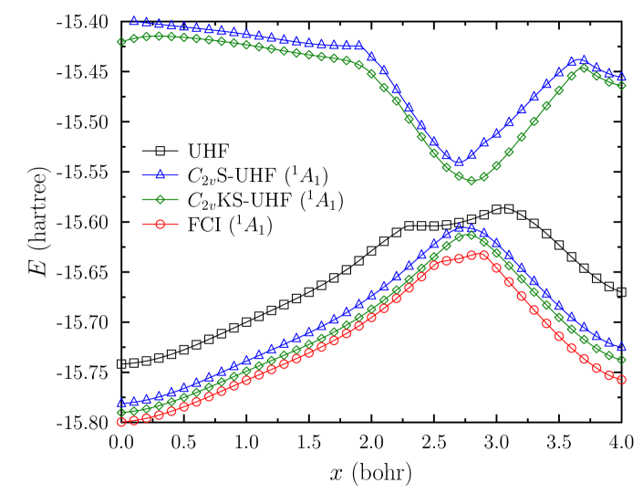
Figure 4: Model $C_{2v}$ insertion pathway of Be into H₂ as a function of the $x$-coordinate of the hydrogen atoms (Be is placed at the origin). The FCI results were obtained from Ref. Evangelista et al., 2006. Note that $C_{2v}$S-UHF and $C_{2v}$KS-UHF predict smooth curves for the two low-lying ${}^{1}A_{1}$ states.

As Fig. 4 shows, both excited symmetry-projected HF approaches provide smooth curves for both the ground state and the first excited state. The obtained curves display the interaction between the lowest ${}^{1}A_{1}$ states in the model reaction pathway. Moreover, the profiles are qualitatively similar to the CASSCF and FCI curves reported in Ref. Purvis, III et al., 1983 for both states. The $C_{2v}$KS-UHF curve lies very close to the FCI curve in the interval $x<2.5$. Near $x\approx 2.7$, where the multi-reference character is expected to be highest as the different configurations interact strongly, both $C_{2v}$S-UHF and $C_{2v}$KS-UHF deviate from the ground state FCI curve. We stress, nevertheless, that our results can be improved by: a) using more symmetry-projected configurations for each state, and b) including more states in the excited symmetry-projected HF approach.

V Conclusions

The spectrum of a molecular system constitutes the fingerprint of its quantum mechanical character. Characterization of the low-lying excited states of a system is of paramount importance in order to understand photochemical and photophysical processes occurring in nature. Accessing an excited state of the same symmetry as the ground state has always been challenging for variational strategies. This is because, if the optimization is carried out using the same formalism as that used for the ground state, a variational collapse is almost inevitable. In the formalism discussed in this work we avoided this collapse by using an ansatz that is explicitly orthogonal to states of the same symmetry previously obtained. We note that the Gram-Schmidt orthogonal construction used in this work in terms of symmetry-projected configurations could be used with other types of wavefunction.

In a nutshell, our formalism uses chain of variational calculations to characterize the low-lying excited states of a system with a given set of quantum numbers in terms of symmetry-projected configurations. The use of the latter implies that the wavefunctions thus obtained have well defined symmetries.

We have applied the excited symmetry-projected HF formalism to describe the dissociation profile of the C₂ molecule, to characterize the low-lying spectrum of formaldehyde, and to explore a model insertion pathway for BeH₂. Several features of the potential energy curve of the carbon dimer were correctly reproduced; in particular, the non-Morse shape of the lowest lying $A_{1}$ state is obtained after the two symmetry-projected configurations are allowed to interact. This constitutes the avoided crossing also observed with other multi-configurational methods such as MRCI or CASPT2. The low-lying singlet and triplet spectrum of formaldehyde was characterized and compared with available experimental adiabatic excitation energies. We have observed a good agreement between our computed spectrum and the experimental one (all excitation energies are correct within a $\approx 1$ eV window). This is remarkable given that each state was essentially described by a single-symmetry projected configuration, that is, we solved for as many states as the amount of symmetry-projected configurations we used.

The methodology here considered can be applied to larger systems as it has mean-field cost. We believe that this method can become a useful tool for the computational chemist. It may be used to fill the void between the high-accuracy methods and the large-scale methods, where the latter typically assume a particle-hole character for the low-lying excited states.

Appendix A Matrix elements between symmetry-projected configurations

In this appendix, we provide explicit expressions for matrix elements required in the evaluation of the energy and the energy gradient of wavefunctions based on symmetry-projected configurations. As shown below, these can be in turn written in terms of matrix elements between (non-orthogonal) rotated Slater determinants. Löwdin Löwdin (1955b) first described the evaluation of arbitrary operator matrix elements between non-orthogonal $N$-electron Slater determinants. An extended Wick’s theorem can be used to evaluate such matrix elements as shown by, e.g., Blaizot and Ripka Blaizot and Ripka (1985).

We begin by describing the notation used. We work with a set of $M$ elementary fermion creation $\{c^{\dagger}\}$ and annihilation $\{c\}$ operators satisfying the standard anti-commutation rules

$$\Big{[}c_{j},c_{k}\Big{]}_{+} =\,0,$$ (30a)

$$\Big{[}c_{j}^{\dagger},c_{k}^{\dagger}\Big{]}_{+} =\,0,$$ (30b)

$$\Big{[}c_{j},c_{k}^{\dagger}\Big{]}_{+} =\,\langle j|k\rangle=\delta_{jk}.$$ (30c)

Note than an orthonormal basis is used. The transformation from the non-orthogonal atomic orbital basis to an orthonormal one is straightforward.

The non-relativistic, Born-Oppenheimer molecular electronic Hamiltonian $\hat{H}$ is expressed in second quantization as

$$\hat{H}=\sum_{ik}\langle i|\hat{h}|k\rangle\,c_{i}^{\dagger}\,c_{k}+\frac{1}{4}\sum_{ijkl}\langle ij|\hat{v}|kl\rangle\,c_{i}^{\dagger}\,c_{j}^{\dagger}\,c_{l}\,c_{k},$$ (31)

where $\langle i|\hat{h}|k\rangle$ are one-electron (core Hamiltonian) integrals and $\langle ij|\hat{v}|kl\rangle$ are anti-symmetrized two-electron (electron repulsion) integrals in Dirac notation.

An arbitrary $N$-electron Slater determinant $|\Phi\rangle$ is constructed as a vacuum to a set of $N$ occupied (hole) HF creation operators $\{b_{h}^{\dagger}\,|\,h=1,\ldots,N\}$ and $M-N$ virtual (particle) HF annihilation operators $\{b_{p}\,|\,p=N+1,\ldots,M\}$. It may be represented as

$$|\Phi\rangle=\prod_{h=1}^{N}b_{h}^{\dagger}|-\rangle,$$ (32)

where $|-\rangle$ is the bare fermion vacuum (annihilated by $\{c\}$). The HF operators are given as linear combinations of the elementary fermion ones, that is,

$$b_{k}^{\dagger}=\sum_{j}D_{jk}^{\ast}\,c_{j}^{\dagger},$$ (33)

where $D$ is the matrix of molecular orbital coefficients. (Note that our choice for the matrix of orbital coefficients is the complex conjugate of the standard one.) As usual, the first $N$ columns in $D$ are used for the occupied molecular orbitals, while the remaining columns describe the virtual orbitals. The above transformation is canonical (it preserves fermion anti-commutation rules) if the matrix $D$ is unitary: $D\,D^{\dagger}=D^{\dagger}\,D=\mathbf{1}$.

In order to provide explicit expressions for the matrix elements, we introduce a generic form of the projection operator $\hat{P}^{j}_{mk}$ (for general non-Abelian groups) given by

$$\hat{P}^{j}_{mk}=\frac{1}{V}\int_{V}d\vartheta\,w^{j}_{mk}(\vartheta)\,\hat{R}(\vartheta).$$ (34)

A state transforming as the $m$-th row of the $j$-th irreducible representation is recovered upon the action of the above projection operator on an arbitrary state. Here, $\vartheta$ labels the elements of the symmetry group; for discrete groups, the integration should be understood as a summation. In addition, $V$ is the volume of integration, $w^{j}_{mk}(\vartheta)$ is an integration weight (character) associated with the symmetries of the state to be recovered, and $\hat{R}(\vartheta)$ is a rotation operator.

For all the cases considered in this work, $\hat{R}(\vartheta)$ is a single-particle rotation operator that transforms the HF operators according to

$$b_{k}^{\dagger}(\vartheta) \equiv\,\hat{R}(\vartheta)\,b_{k}^{\dagger}\,\hat{R}^{-1}(\vartheta)$$

$$=\,\sum_{j}D_{jk}^{\ast}\,\hat{R}(\vartheta)\,c_{j}^{\dagger}\,\hat{R}^{-1}(\vartheta)=\sum_{ji}D_{jk}^{\ast}\,R_{ij}(\vartheta)\,c_{i}^{\dagger},$$ (35)

where $R_{ij}(\vartheta)=\langle i|\hat{R}(\vartheta)|j\rangle$ is an element of the matrix representation of the rotation operator in the single-particle basis.

Using Eq. 34, overlap and Hamiltonian matrix elements between symmetry-projected configurations are expressed in terms of norm and Hamiltonian overlaps between rotated determinants $\hat{R}(\vartheta)|\Phi\rangle$ as

$$\langle\Phi^{r}|\hat{P}^{j}_{kk^{\prime}}|\Phi^{s}\rangle =\,\frac{1}{V}\int_{V}d\vartheta\,w^{j}_{kk^{\prime}}(\vartheta)\,n^{rs}(\vartheta),$$ (36a)

$$\langle\Phi^{r}|\hat{H}\,\hat{P}^{j}_{kk^{\prime}}|\Phi^{s}\rangle =\,\frac{1}{V}\int_{V}d\vartheta\,w^{j}_{kk^{\prime}}(\vartheta)\,n^{rs}(\vartheta)\,h^{rs}(\vartheta),$$ (36b)

where

$$n^{rs}(\vartheta) \equiv\,\langle\Phi^{r}|\hat{R}(\vartheta)|\Phi^{s}\rangle,$$ (37a)

$$h^{rs}(\vartheta) \equiv\,\frac{\langle\Phi^{r}|\hat{H}\,\hat{R}(\vartheta)|\Phi^{s}\rangle}{\langle\Phi^{r}|\hat{R}(\vartheta)|\Phi^{s}\rangle}.$$ (37b)

The norm overlaps of Eq. 37a can be evaluated by applying Wick’s theorem on the bare fermion vacuum. This leads to

$$n^{rs}(\vartheta) =\,\mathrm{det}_{N}\,X^{rs}(\vartheta),$$ (38)

$$X^{rs}(\vartheta) =\,D^{r\mathsf{T}}\,R(\vartheta)\,D^{s\ast}.$$ (39)

Here, $D^{k}$ is the (rectangular) matrix of occupied orbital coefficients associated with the determinant $|\Phi^{k}\rangle$ and $R(\vartheta)$ is the matrix representation of the rotation operator in the single-particle basis. The notation $\mathrm{det}_{N}$ is used to emphasize that the determinant should be evaluated over the $N\times N$ block of $X^{rs}(\vartheta)$ defined by the occupied states in $|\Phi^{r}\rangle$ and $|\Phi^{s}\rangle$.

The Hamiltonian overlaps of Eq. 37b can be evaluated by using an extended Wick’s theorem Blaizot and Ripka (1985) when $|\Phi^{r}\rangle$ and $|\Phi^{s}\rangle$ are not orthogonal. They are given by

$$h^{rs}(\vartheta) =\,\sum_{ik}\left[\langle i|\hat{h}|k\rangle+\frac{1}{2}\,\Gamma^{rs}_{ik}(\vartheta)\right]\rho^{rs}_{ki}(\vartheta),$$ (40)

$$\Gamma^{rs}_{ik}(\vartheta) =\,\sum_{jl}\langle ij|\hat{v}|kl\rangle\,\rho^{rs}_{lj}(\vartheta).$$ (41)

The Hamiltonian overlaps are expressed in terms of the transition density matrix $\rho^{rs}(\vartheta)$, with elements defined by

$$\rho^{rs}_{ki}(\vartheta)\equiv\frac{\langle\Phi^{r}|c_{i}^{\dagger}\,c_{k}\,\hat{R}(\vartheta)|\Phi^{s}\rangle}{\langle\Phi^{r}|\hat{R}(\vartheta)|\Phi^{s}\rangle}.$$ (42)

The transition density matrix of Eq. 42 is built according to Löwdin (1955b)

$$\rho^{rs}(\vartheta)=R(\vartheta)\,D^{s\ast}\,\left[X^{rs}(\vartheta)\right]^{-1}\,D^{r\mathsf{T}}.$$ (43)

Here, the inverse of $X^{rs}(\vartheta)$ (defined in Eq. 39) should be evaluated over the $N\times N$ block of occupied states in both determinants. Accordingly, only the occupied orbitals in $D^{r}$ and $D^{s}$ should be used in computing the matrix product above.

Matrix elements appearing in contributions to the energy gradient can also be expressed in terms of overlaps between rotated determinants:

$$\langle\Phi^{r}|b_{h}^{r\dagger}\,b_{p}^{r}\,\hat{P}^{j}_{kk^{\prime}}|\Phi^{s}\rangle =\,\frac{1}{V}\int_{V}d\vartheta\,w^{j}_{kk^{\prime}}(\vartheta)\,n^{rs}(\vartheta)\,N^{rs}_{ph}(\vartheta),$$ (44a)

$$\langle\Phi^{r}|b_{h}^{r\dagger}\,b_{p}^{r}\,\hat{H}\,\hat{P}^{j}_{kk^{\prime}}|\Phi^{s}\rangle =\,\frac{1}{V}\int_{V}d\vartheta\,w^{j}_{kk^{\prime}}(\vartheta)\,n^{rs}(\vartheta)\,H^{rs}_{ph}(\vartheta),$$ (44b)

where we have appended a superscript to the HF operators to label the determinant to which they are associated. Here,

$$N^{rs}_{ph}(\vartheta) \equiv\,\frac{\langle\Phi^{r}|b_{h}^{r\dagger}\,b_{p}^{r}\,\hat{R}(\vartheta)|\Phi^{s}\rangle}{\langle\Phi^{r}|\hat{R}(\vartheta)|\Phi^{s}\rangle},$$ (45a)

$$H^{rs}_{ph}(\vartheta) \equiv\,\frac{\langle\Phi^{r}|b_{h}^{r\dagger}\,b_{p}^{r}\,\hat{H}\,\hat{R}(\vartheta)|\Phi^{s}\rangle}{\langle\Phi^{r}|\hat{R}(\vartheta)|\Phi^{s}\rangle}.$$ (45b)

The matrix elements of Eq. 45 can be evaluated using an extended Wick’s theorem when $|\Phi^{r}\rangle$ and $|\Phi^{s}\rangle$ are not orthogonal. They are given by

$$N^{rs}_{ph}(\vartheta) =\,\left[D^{r\mathsf{T}}\,\rho^{rs}(\vartheta)\,D^{r\ast}\right]_{ph},$$ (46a)

$$H^{rs}_{ph}(\vartheta) =\,h^{rs}(\vartheta)\left[D^{r\mathsf{T}}\,\rho^{rs}(\vartheta)\,D^{r\ast}\right]_{ph}$$

$$+\,\left[D^{r\mathsf{T}}\,\left(\mathbf{1}-\rho^{rs}(\vartheta)\right)\,f^{rs}(\vartheta)\,\rho^{rs}(\vartheta)\,D^{r\ast}\right]_{ph},$$ (46b)

where we have set $f^{rs}_{ik}(\vartheta)=\langle i|\hat{h}|k\rangle+\Gamma^{rs}_{ik}(\vartheta)$.

References

- Dreuw and Head-Gordon (2005) A. Dreuw and M. Head-Gordon, Chem. Rev. 105, 4009 (2005).
- Werner and Meyer (1981) H.-J. Werner and W. Meyer, J. Chem. Phys. 74, 5794 (1981).
- Roos et al. (1996) B. O. Roos, K. Andersson, M. P. Fülscher, P. Å. Malmqvist, L. Serrano-Andrés, K. Pierloot, and M. Merchán, in Advances in Chemical Physics: New Methods in Computational Quantum Mechanics, Vol. 93, edited by I. Prigogine and S. A. Rice (Wiley, New York, 1996) pp. 219–231.
- Krylov (2008) A. I. Krylov, Annu. Rev. Phys. Chem. 59, 433 (2008).
- Watts (2008) J. D. Watts, in Radiation Induced Molecular Phenomena in Nucleic Acids: A Comprehensive Theoretical and Experimental Analysis, edited by M. K. Shukla and J. Leszczynski (Springer, 2008) pp. 65–92.
- Li and Paldus (2011) X. Li and J. Paldus, J. Chem. Phys. 134, 214118 (2011).
- Ivanov et al. (2011) V. V. Ivanov, D. I. Lyakh, and L. Adamowicz, Annu. Rep. Prog. Chem., Sect. C: Phys. Chem. 107, 169 (2011).
- Nakatsuji (1979) H. Nakatsuji, Chem. Phys. Lett. 67, 329 (1979).
- Rohlfing (2000) M. Rohlfing, Int. J. Quantum Chem. 80, 807 (2000).
- Kuś et al. (2009) T. Kuś, V. F. Lotrich, and R. J. Bartlett, J. Chem. Phys. 130, 124122 (2009).
- Casida and Huix-Rotllant (2012) M. E. Casida and M. Huix-Rotllant, Annu. Rev. Phys. Chem. 63, 287 (2012).
- Foresman et al. (1992) J. B. Foresman, M. Head-Gordon, J. A. Pople, and M. J. Frisch, J. Phys. Chem. 96, 135 (1992).
- Schmid et al. (1986) K. W. Schmid, F. Grümmer, M. Kyotoku, and A. Faessler, Nucl. Phys. A 452, 493 (1986).
- Schmid (2004) K. W. Schmid, Prog. Part. Nucl. Phys. 52, 565 (2004).
- Rodríguez-Guzmán et al. (2012) R. Rodríguez-Guzmán, K. W. Schmid, C. A. Jiménez-Hoyos, and G. E. Scuseria, Phys. Rev. B , 245130 (2012).
- Rodríguez-Guzmán et al. (2013) R. Rodríguez-Guzmán, C. A. Jiménez-Hoyos, R. Schutski, and G. E. Scuseria, Phys. Rev. B 87, 235129 (2013).
- Löwdin (1955a) P.-O. Löwdin, Phys. Rev. 97, 1509 (1955a).
- Löwdin (1966) P.-O. Löwdin, in Quantum Theory of Atoms, Molecules, and the Solid State: A Tribute to John C. Slater, edited by P.-O. Löwdin (Academic Press, New York, 1966) pp. 601–623.
- Jiménez-Hoyos et al. (2012a) C. A. Jiménez-Hoyos, T. M. Henderson, T. Tsuchimochi, and G. E. Scuseria, J. Chem. Phys. 136, 164109 (2012a).
- Bayman (1960) B. F. Bayman, Nucl. Phys. 15, 33 (1960).
- Villars (1966) F. Villars, in Varenna Lectures, Vol. 36, edited by C. Bloch (Academic Press, New York, 1966) p. 1.
- Percus and Rotenberg (1962) J. K. Percus and A. Rotenberg, J. Math. Phys. 3, 928 (1962).
- Ring and Schuck (1980) P. Ring and P. Schuck, The Nuclear Many-Body Problem (Springer-Verlag, Berlin, 1980).
- Note (1) Here, may stand for a product of projection operators for say, spin and point group restoration.
- Schmid et al. (1984) K. W. Schmid, F. Grümmer, and A. Faessler, Phys. Rev. C 29, 291 (1984).
- Schlegel (1986) H. B. Schlegel, J. Chem. Phys. 84, 4530 (1986).
- Mayer (1980) I. Mayer, Adv. Quantum Chem. 12, 189 (1980).
- Mang (1975) H. J. Mang, Phys. Rep. 18, 325 (1975).
- Noga and Šimunek (2010) J. Noga and J. Šimunek, J. Chem. Theory Comput. 6, 2706 (2010).
- Backsay (1981) G. B. Backsay, Chem. Phys. 61, 385 (1981).
- Egido et al. (1995) J. L. Egido, J. Lessing, V. Martin, and L. M. Robledo, Nucl. Phys. A 594, 70 (1995).
- Jiménez-Hoyos (2013) C. A. Jiménez-Hoyos, Variational approaches to the molecular electronic structure problem based on symmetry-projected Hartree–Fock configurations, Ph.D. thesis, Rice University (2013).
- Jiménez-Hoyos et al. (2012b) C. A. Jiménez-Hoyos, R. Rodríguez-Guzmán, and G. E. Scuseria, Phys. Rev. A 86, 052102 (2012b).
- Nocedal and Wright (2006) J. Nocedal and S. J. Wright, Numerical Optimization, 2nd ed., Springer Series in Operations Research and Financial Engineering (Springer, New York, 2006).
- Jiménez-Hoyos et al. (2013) C. A. Jiménez-Hoyos, R. Rodríguez-Guzmán, and G. E. Scuseria, J. Chem. Phys. (2013), submitted.
- Fukutome (1988) H. Fukutome, Prog. Theor. Phys. 80, 417 (1988).
- Schmid et al. (1989) K. W. Schmid, Z. Ren-Rong, F. Grümmer, and A. Faessler, Nucl. Phys. A 499, 63 (1989).
- Koch and Dalgaard (1993) H. Koch and E. Dalgaard, Chem. Phys. Lett. 212, 193 (1993).
- Nocedal (1980) J. Nocedal, Math. Comput. 35, 773 (1980).
- Liu and Nocedal (1989) D. C. Liu and J. Nocedal, Math. Program. 45, 503 (1989).
- (41) M. J. Frisch, G. W. Trucks, H. B. Schlegel, G. E. Scuseria, M. A. Robb, J. R. Cheeseman, G. Scalmani, V. Barone, B. Mennucci, G. A. Petersson, H. Nakatsuji, M. Caricato, X. Li, H. P. Hratchian, A. F. Izmaylov, J. Bloino, G. Zheng, J. L. Sonnenberg, M. Hada, M. Ehara, K. Toyota, R. Fukuda, J. Hasegawa, M. Ishida, T. Nakajima, Y. Honda, O. Kitao, H. Nakai, T. Vreven, J. A. Montgomery, Jr., J. E. Peralta, F. Ogliaro, M. Bearpark, J. J. Heyd, E. Brothers, K. N. Kudin, V. N. Staroverov, R. Kobayashi, J. Normand, K. Raghavachari, A. Rendell, J. C. Burant, S. S. Iyengar, J. Tomasi, M. Cossi, N. Rega, J. M. Millam, M. Klene, J. E. Knox, J. B. Cross, V. Bakken, C. Adamo, J. Jaramillo, R. Gomperts, R. E. Stratmann, O. Yazyev, A. J. Austin, R. Cammi, C. Pomelli, J. W. Ochterski, R. L. Martin, K. Morokuma, V. G. Zakrzewski, G. A. Voth, P. Salvador, J. J. Dannenberg, S. Dapprich, A. D. Daniels, Ã. Farkas, J. B. Foresman, J. V. Ortiz, J. Cioslowski, and D. J. Fox, Gaussian Development Version, Revision H.1, Gaussian Inc., Wallingford, CT, 2009.
- Abrams and Sherrill (2004) M. L. Abrams and C. D. Sherrill, J. Chem. Phys. 121, 9211 (2004).
- Sherrill and Piecuch (2005) C. D. Sherrill and P. Piecuch, J. Chem. Phys. 122, 124104 (2005).
- Robin (1985) M. B. Robin, Higher Excited States of Polyatomic Molecules, Vol. 3 (Academic Press, New York, 1985).
- Taylor et al. (1982) S. Taylor, D. G. Wilden, and J. Comer, Chem. Phys. 70, 291 (1982).
- Hadad et al. (1993) C. M. Hadad, J. B. Foresman, and K. B. Wiberg, J. Phys. Chem. 97, 4293 (1993).
- Pitarch-Ruiz et al. (2003) J. Pitarch-Ruiz, J. Sánchez-Marín, A. Sánchez de Meras, and D. Maynau, Mol. Phys. 101, 483 (2003).
- Schreiber et al. (2008) M. Schreiber, M. R. Silva-Junior, S. P. A. Sauber, and W. Thiel, J. Chem. Phys. 128, 134110 (2008).
- Note (2) This, however, does not imply that all the triplet components in a symmetry-projected construction are not degenerate. If a UHF-type determinant has , then all states of the form , with , are degenerate.
- Daudey et al. (1993) J.-P. Daudey, J.-L. Heully, and J.-P. Malrieu, J. Chem. Phys. 99, 1240 (1993).
- Purvis, III et al. (1983) G. D. Purvis, III, R. Shepard, F. B. Brown, and R. J. Bartlett, Int. J. Quantum Chem. 23, 835 (1983).
- Evangelista et al. (2006) F. A. Evangelista, W. D. Allen, and H. F. Schaefer, III, J. Chem. Phys. 125, 154113 (2006).
- Löwdin (1955b) P.-O. Löwdin, Phys. Rev. 97, 1490 (1955b).
- Blaizot and Ripka (1985) J.-P. Blaizot and G. Ripka, Quantum Theory of Finite Systems (The MIT Press, Cambridge, MA, 1985).