To Stack or Not to Stack:
Spectral Energy Distribution Properties of Ly$\alpha$-Emitting Galaxies at $z$ $=$ 2.1

Abstract

We use the Cosmic Assembly Near-Infrared Deep Extragalactic Legacy Survey (CANDELS) GOODS-S multi-wavelength catalog to identify counterparts for 20 Ly$\alpha$ Emitting (LAE) galaxies at $z=2.1$. We build several types of stacked Spectral Energy Distributions (SEDs) of these objects. We combine photometry to form average and median flux-stacked SEDs, and postage stamp images to form average and median image-stacked SEDs. We also introduce scaled flux stacks that eliminate the influence of variation in overall brightness. We use the SED fitting code SpeedyMC to constrain the physical properties of individual objects and stacks. Our LAEs at $z=2.1$ have stellar masses ranging from $2\times 10^{7}$ $M_{\odot}$ - $8\times 10^{9}$ $M_{\odot}$ (median $=3\times 10^{8}M_{\odot}$), ages ranging from 4 Myr to 500 Myr (median =100 Myr), and E(B-V) between 0.02 and 0.24 (median = 0.12). We do not observe strong correlations between Ly$\alpha$ equivalent width (EW) and stellar mass, age, or E(B-V). The Ly$\alpha$ radiative transfer ($q$) factors of our sample are predominantly close to one and do not correlate strongly with EW or E(B-V), implying that Ly$\alpha$ radiative transfer prevents Ly$\alpha$ photons from resonantly scattering in dusty regions. The SED parameters of the flux stacks match the average and median values of the individual objects, with the flux-scaled median SED performing best with reduced uncertainties. Median image-stacked SEDs provide a poor representation of the median individual object, and none of the stacking methods captures the large dispersion of LAE properties.

1. Introduction

Lyman Alpha Emitting (LAE) galaxies at $2<z<3$ are thought to be building blocks of present-day galaxies like our own Milky Way (Gawiser et al., 2007; Guaita et al., 2011). These galaxies are easy to detect thanks to the strength of the Lyman-$\alpha$ (Ly$\alpha$) line, but they usually have low stellar masses and are therefore dim in the continuum. As a result, it has been a common procedure to stack multiple photometric data points of LAEs in order to enhance their signal-to-noise ratio (Gawiser et al., 2006a, 2007; Nilsson et al., 2007; Pirzkal et al., 2007; Finkelstein et al., 2007; Lai et al., 2008; Pentericci et al., 2008; Ono et al., 2010b, a; Ouchi et al., 2010; Nilsson et al., 2011; Guaita et al., 2011; Finkelstein et al., 2011a; Acquaviva et al., 2011, 2012b).

The nature of radiation emitted from astrophysical sources offers insights into their physical properties. Ly$\alpha$ photons are emitted when a neutral hydrogen atom undergoes a transition from the first excited state to the ground state. An immense number of Ly$\alpha$ photons are emitted at 1216 $\AA$ rest frame from HII regions surrounding young, massive stars. The large luminosity of the Ly$\alpha$ emission line makes it easily identified even over vast distances and thus it is widely used in research in extragalactic astronomy. LAEs are typically discovered using the narrow-band filter technique (Cowie & Hu, 1998; Rhoads et al., 2000), in which a detection of an LAE is made by finding greater signal to noise ratios in a narrow-band filter image than in images obtained with adjacent broad-band filters.

Inconsistencies in the literature, particularly in estimating ages and sample diversity, motivate a study of the validity of the stacking method for analyzing the Spectral Energy Distributions (SEDs) of dim LAEs. To date, most SED studies of high-redshift LAEs have been done by stacking the catalog fluxes or ground-based postage stamp images of galaxies too faint to study individually. By stacking numerous faint objects (via average or median) we increase the signal to noise significantly. It is believed that a study of these images will represent the characteristics of a sample of galaxies on the average. However, this interpretation of median as typical relies on the assumption that the best fit SED parameters of the stacked galaxies have similar physical properties. An additional key assumption is that the median (average) SEDs will match the median (average) physical properties of individual galaxy SEDs. This assumption appears reasonable for stellar mass if the mass to light ratio of the stellar populations of different LAEs is similar, but it is not guaranteed for other parameters like age or dust. In conjunction with this study, a study by Hagen, A., et al. (2013, in prep.), in which LAEs identified by the Hobby-Eberly Telescope Dark Energy eXperiment (HETDEX) pilot survey are studied individually through SED fitting, could shed more light on these inconsistencies.

Results from the analysis of stacked samples of LAEs indicate a large spread in the properties of these galaxies and introduce further concern about the validity of the stacking technique. A recent study of median image-stacked LAEs at z = 3.1 found them to be older than median flux-stacked LAEs at z = 2.1 (Acquaviva et al., 2012a); this puzzling result would imply that LAEs grow younger as cosmic time progresses. However, it might instead result from the failure of image and/or flux stacking to accurately measure the SED characteristics of individual galaxies, and from systematic differences between image-stacking and flux-stacking. Additionally, a previous study of individual LAEs at $z=4.5$ (Finkelstein et al., 2009) found a wide range of physical properties, including many LAEs which appeared dusty, something that would not have been expected given the earlier results at $z=3.1$ from Gawiser et al. (2006b) which implied, via a stacking analysis, that LAEs were dust free.

In this paper, we perform SED fitting on 20 LAEs at $z=2.1$ as well as on their flux- and image-stacked SEDs, in order to clarify whether these discrepancies are attributable to the failure of one or all stacking methods. The use of deep HST and Spitzer IRAC data gives us the opportunity, for the first time, to study rest-frame ultra-violet and optical properties of individual objects, which is crucial for accurate constraints on age and stellar mass. We use the Markov Chain Monte Carlo (MCMC) algorithm ¡ÈSpeedyMC¡É (Acquaviva et al., 2012a) to analyze the SED properties of our sample. SpeedyMC is a streamlined implementation of GalMC (Acquaviva et al., 2011) designed to handle large samples of SEDs. This code utilizes Bayesian statistics to determine the expectation values of SED parameters and provide estimates of the uncertainties associate to their measurements. All SED fitting calculations assume a WMAP-based cosmology including $H_{0}=73$ km s^-1 Mpc^-1

2. Data

The starting point for our analysis was the sample of 216 LAE candidates at $z=2.1$ discovered in deep 3727 Å narrow-band images of the 30^′ $\times$ 30^′ Extended Chandra Deep Field-South (ECDF-S) by Guaita et al. (2010) as refined by Bond et al. (2012), who excluded 34 additional LAE candidates that appear to be low-redshift contaminants due to extended morphology in HST images. These objects typically have low signal to noise ratios in ground-based broad-band images, with a median magnitude of $R\sim 25.5$ and are unresolved at 0.1 arcseconds. Thus, the addition of deep HST imaging is crucial.

CANDELS has produced a deep H-band-selected multiwavelength catalog of the GOODS-S field, which encompasses the central $16^{\prime}\times 10^{\prime}$ of ECDF-S (Guo et al., 2013). The observations are 10 epochs deep in H band, which corresponds to roughly six HST orbits. The catalog contains photometry from $U$-band images from CTIO and VIMOS, ACS ($BViz$) images from the GOODS survey (Giavalisco et al., 2004), CANDELS WFC3 images (F098M,$YJH$), $K$-band images from Hawk-I and ISAAC, and Spitzer Space Telescope Infrared Array Camera (IRAC; Fazio et al. 2004) 3.6, 4.5 $\mu$m images from SEDS (Ashby et al., 2013) and 5.8, 8.0 $\mu$m images from GOODS (Dickinson et al., 2003). For SED fitting, we excluded both U bands due to expected Ly$\alpha$ contamination at this redshift, F098M due to having coverage in a minority of our sample, and both K-bands due to incomplete coverage and shallower photometry. All of our analysis made use of imaging and photometry from the remaining 11 space-based bands.

We match the positions of our catalog of known LAEs at z=2.1 to the positions of objects contained within the version of the CANDELS Multi-wavelength catalog presented in Guo et al. (2013). Objects within a distance of $0.5$ arcseconds were recorded as a match, and their CANDELS SEDs were used in our analysis. Only two objects showed multiple possible counterparts within this tolerance, and they were discarded due to the strong likelihood of neighboring object contamination. In total, we found 20 LAE counterparts in the CANDELS Multi-wavelength catalog. We note that only 30 of the original 216 LAEs are within the GOODS-S field, and the 10 “missing” objects were probably too dim to have been detected at the 5$\sigma$ level in H band, and were thus excluded from the CANDELS catalog.

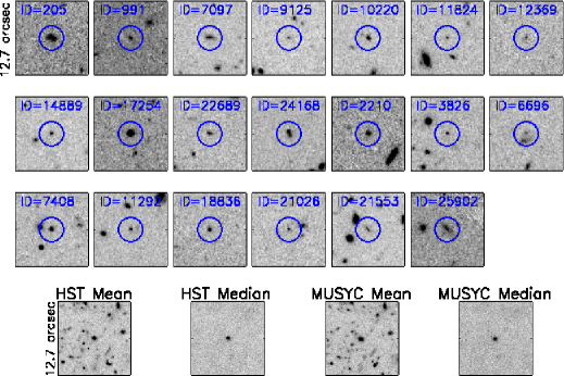
Figure 1.— HST F160W filter postage stamp images of the 20 individual objects and image stacks in our sample. HST stacks are obtained from centroiding on the CANDELS object positions, while NB-centered stacks are obtained from centroiding on the MUSYC NB positions. The blue circles highlight the objects to aid the eye. In these stamps, North points to the top of the page, and East points to the right. All Stamp images are square of side length $12.7\arcsec$.

The main objective of this paper is the comparison of the SED fitting properties of individual objects and stacks. The SEDs of the stacks can be obtained via two different procedures: by combining the cataloged fluxes of the individual objects, or by stacking the postage-stamp images of the 20 individual objects at each wavelength and then performing photometry on the combined images. We refer to the SEDs obtained via these two methods as “flux-stacked” and “image-stacked” respectively. We took the median and average of the flux densities in each band of all 20 $z=2.1$ LAEs with CANDELS counterparts and will henceforth refer to these as the median and average flux stacks respectively.

To create the image-stacked SED, we performed both average and median stacking from cutout images centered around each of our 20 LAEs. The extracted HST cutouts measured 211 pixels on a side, while the IRAC cutouts measured 21 pixels. As the processed HST image pixels measure 0.06^′′ and the processed IRAC image pixels measure 0.6^′′, the cutouts in all bands had approximately the same size of 12.6^′′ on a side. We note that of the 20 objects, 6 of them were located in the northern $\sim$25% of the GOODS-S field, which has WFC3 data from the WFC3 Early Release Science program (ERS; Windhorst et al. 2011). While these images were obtained prior to the CANDELS data, they were reprocessed alongside the CANDELS data to make a single mosaic which was used to extract the cutouts. Along with the science images, we also extracted cutouts from the r.m.s. images for use with Source Extractor (Bertin & Arnouts 1996, see Koekemoer et al. 2011 for details on the science and r.m.s. mosaic construction).

To create our image stacks, we created median and average images by taking the median/average value for each pixel from all of the cutout images for a given band, excluding pixels with r.m.s. values $>$ 10; a very high value, indicative of a problem with the given pixel in that image. We then measured photometry on the image stacks using Source Extractor in dual-image mode, with the F160W stack as the detection image for the HST bands and the 3.6 $\mu$m image as the detection band for the IRAC images. We measured photometry using Kron-style elliptical apertures, denoted by MAG_AUTO within Source Extractor. For the HST bands, we measured colors in small Kron apertures (with the parameter PHOT_AUTOPARAMS set to 1.2, 1.7), with the fluxes corrected to total using an aperture correction derived by the ratio of the default MAG_AUTO flux value to our smaller Kron flux (this procedure has been optimized for faint, high-redshift sources; see Finkelstein et al. 2010 for details). For the IRAC stacks, we simply measured photometry in the larger Kron aperture, which is designed to approximate a total flux. The photometry for the individual objects was also performed in the same way.

To further our analysis we also introduce an additional set of image stacks centered on the object positions found in the MUSYC narrow-band (NB) catalog of LAEs. Comparison of the primary HST-centered image stacks with these NB-centered stacked images will illustrate any improvement that results from eliminating the $\sim 0.1^{\prime\prime}$ narrow-band centroiding errors (Guaita et al., 2010) and any astrometric offsets between ground-based and space-based coordinates. Figure 1 shows F106W filter postage stamp images of each galaxy in our sample and those of the HST and NB-centered image stacks. In order to explore the effects of potential IRAC contamination, we introduce IRAC-clean image stacks. These stacks were comprised of ten individual objects visually deemed clean in the IRAC 3.6$\mu m$ band. The IRAC-clean stack postage stamp images are compared to those of the entire sample in Figure 2. A slight loss of S/N in the clean sample is apparent due to the reduced sample size. Figure 3 shows the SEDs of all individual objects and all stacks overlaid atop one-another for comparison. We also introduce a subsample of our 20 LAEs that were visually deemed “clean”, or free of nearby sources in the IRAC $3.6\mu m$ band. Of the original 20 LAEs in our sample, 11 of them comprise the IRAC-clean sample.

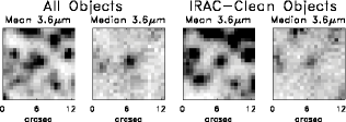
Figure 2.— Average and median postage stamp images for the entire sample and the sample deemed clean in the IRAC $3.6\mu m$ band. Note the reduced signal to noise in the clean median image; an effect of its lower sample size.

2.1. Error estimation

The uncertainty in the fluxes for individual objects’ SEDs include both a photometric error and a zero-point error arising from the combination of calibration and zero-point errors; these are added in quadrature. We assume the calibration error to be 3% in HST bands and 8% for the IRAC bands (CANDELS team, private communication).

Errors on the flux-stacked photometry are determined by a bootstrap procedure, as in Guaita et al. (2011) and Acquaviva et al. (2011). This accounts for both the photometric error and the sample variance resulting from the spread in the SEDs of different galaxies; for our sample, the latter is the dominant source of uncertainty. The same calibration uncertainty used for the individual objects’ SED is added in quadrature to the bootstrap error in both the average and median flux stacked SED. For image-stacked SEDs, we adopt a conservative error estimate in each band by taking the larger of the photometric error indicated by SExtractor and the bootstrap error, and adding it in quadrature to the calibration error.

2.2. Stacking Simulations

In order to determine the expected impact of flux- and image-stacking on photometry in a given band, we conducted a series of Monte Carlo simulations. We modeled the behavior in WFC3 NIR images, with 0.06$"$ pixels sampling a 0.18$"$ PSF. A realistic power-law flux distribution was assigned, with fluxes ranging over a factor of 30 distributed uniformly in log(flux). The median of this distribution is only 63% of its average. We then varied the relative level of errors in centroiding, background subtraction, and photometry to check their influence on the resulting average- and median-stacked fluxes. The typical circular aperture used for photometry recovers 71% of the input flux, and we assume hereafter that this can be corrected to produce an unbiased estimate of total flux. Doing so, without any sources of error, both flux stacks and HST-centered image stacks are unbiased in their estimations of median and average flux. Adding a low level of photometric error so that the median object is detected at $S/N\sim 10$ makes no significant difference; this is realistic for H-band where the catalog was detected.

However, centroiding errors are inevitable; for CANDELS objects detected at $S/N>5$, these errors should be at most a single pixel (Koekemoer et al., 2012). When we simulate 1 pixel r.m.s. centroiding errors but no additional sources of error, the average flux and average HST-centered image stacks lose 24% of the flux, the median flux stack loses 29% and the median HST-centered image stack loses 43% of the flux. Adding realistic levels of photometric and background subtraction errors makes no significant difference in these results. The larger flux loss in median image stacks may explain why these are the dimmest stacked SEDs at wavelengths imaged by HST, as seen in Figure 3.

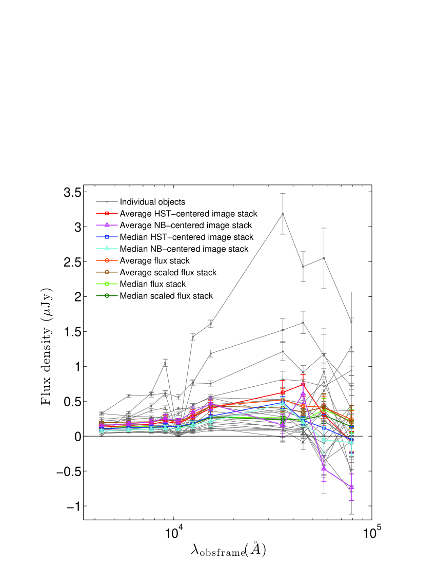
Figure 3.— Above, the SEDs of each individual object (gray) are plotted with all of the stacked SEDs in our analysis. Red is the average HST image stack, blue is the median HST image stack, magenta is the average NB-centered image stack, cyan is the median NB-centered image stack, green is the median flux stack, orange is the average flux stack, brown is the average scaled flux stack, and dark green is the median scaled flux stack. One can observe the median flux stack’s robustness to outlying sources, especially in the Spitzer IRAC bands.

The overall stacking behavior is similar at the much larger pixel scale of IRAC bands (e.g., 1.2$"$ pixels sampling a 1.8$"$ PSF at 3.6 microns), where we continued to assume that the centroiding errors were no larger than 0.06$"$ given the usage of CANDELS H-band catalog positions for the HST-centered image stacks and for TFIT photometry on IRAC images used to make the multiwavelength catalog inputs for flux-stacking. These centroiding errors cause no measurable loss in flux at IRAC resolution. However, this could create a mild color bias in the stacks since, as noted above, 24-43% of the flux is being lost to centroiding errors in HST bands. The worst effect is expected in the median HST-centered image stack, which does exhibit a red $H-$[3.6] color in Fig. 3. It should be noted that our simulations do not include the non-Gaussian PSF wings typical in IRAC bands or any attempt to account for the contamination by neighboring objects that results from them.

We also simulated the NB-centered image stacks where the ground-based MUSYC narrow-band-detected LAE positions were adopted, causing 0.1$"$ centroid errors. If we had used $\sim$FWHM diameter apertures, which are formally optimal for point sources, in the HST images, the NB-centered average (median) stacks would underestimate HST-band fluxes by a factor of 2 (6). However, the larger apertures used in $H$-band to determine aperture corrections are big enough to correct this bias for the average NB-centered image stack, which is well worth the loss of S/N.

It is important to note that no matter what aperture size is used, our simulations show that median image stack photometry is biased low by a large factor whenever centroiding errors are significant compared to the PSF. This occurs because the various objects exhibit only partial overlap, leading median image values to be dominated by image background rather than objects. This provides a significant note of caution about the usage of median image stacks, although the effect appears to be modest for our NB-centered median image stack and should be negligible for our HST-centered median image stack due to the small expected centroiding errors.

3. SED Fitting Methodology

Information about the physical properties of galaxies, including redshift, stellar mass, age, dust content, and metallicity, can be determined by fitting their SEDs. The algorithm that was used for this analysis, SpeedyMC, is a faster version of GalMC introduced in Acquaviva et al. (2012a). Rather than using GALAXEV to generate the model SED at each point, a template library on a grid of locations encompassing the entire parameter space is generated beforehand. The exploration of parameter space is then carried out using the same MCMC algorithm, but at each location, multi-linear interpolation between the pre-computed spectra is used to calculate the model SED and its corresponding $\chi^{2}$ value. The use of SpeedyMC method allows us to fit the SEDs of galaxies at a rate 20,000 times faster than GalMC, and corresponding to about one second per galaxy on a 2.2GHz MacBook Pro laptop.

In our analysis, the parameter space consisted of stellar mass, age, and dust reddening defined by excess color E(B-V). We assumed a constant star formation history, and fixed the metallicity, $Z$, at the value of 0.2$Z_{\odot}$ as indicated by both spectroscopic analysis and SED fitting results (Acquaviva et al., 2011; Finkelstein et al., 2011b). We used the stellar population synthesis models of Bruzual & Charlot (2003) (hereafter BC03) and Charlot & Bruzual (2007, Private Comm.) (hereafter CB07), and included nebular emission according to the procedure described in Acquaviva et al. (2011). Galactic absorption was taken into account using the Calzetti law (Calzetti et al., 1994), with a value $R_{V}=4.05$, and starlight absorption by the IGM using the prescription from Madau (1995). We used the Salpeter initial mass function for consistency with the previous literature on this subject, and assumed a WMAP cosmology. Our reference grid contained 100 values of both age and E(B-V) (the stellar mass is a free normalization parameter which can be varied without the need to build extra models in the grid). The number of values in the grid was chosen by refining the resolution of the grid until the resulting probability distributions obtained from GalMC and SpeedyMC were virtually identical, a sign that the linear interpolation between reference SED was working correctly. We limit the size of the grid in age to be between $10^{6}$ and $3.2\times 10^{9}$ years, as the universe at $z=2.1$ is $3.2\times 10^{9}$ years old. In mass, we limit the grid to range $10^{4}$ and $10^{15}$ $M_{\odot}$, and in E(B-V) we range $0$ to $1$. We ran six chains on each object, using $100,000$ steps for each and starting from six different locations to ensure sampling of the entirety of parameter space and minimize “chain locking” in local minima. The “GetDist” software from Lewis & Bridle (2002) was used to analyze the chains and to make sure that the distribution inferred from the chains had converged to the true one. In the left panel of Figure 4, we plot the observed SED of CANDELS object 3826 overlaid with its best-fitting model produced by SpeedyMC. A similar plot for the median flux stacked SED is included as the right panel of Figure 4. We plot the observed U-band data points in this figure as an illustration of possible Ly$\alpha$ contamination in that band.

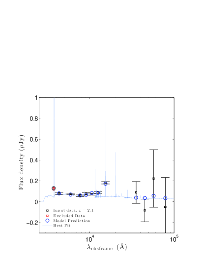
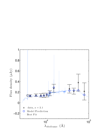
Figure 4.— Top panel:A plot of the SED of individual object 3826 overlaid with its MCMC best fit SED template. These templates correspond to the model SED which produces the lowest $\chi^{2}$ value by SpeedyMC. Note the $U$-band data is affected by Ly$\alpha$ emission and that the emission-line contribution is, in this case, predicted extremely well by the best-fit model to the 11 space-based bands used for SED fitting. Bottom panel: A similar plot for the median flux stack.

4. Results

The BC03 stellar population synthesis models performed better than the CB07 ones, resulting in smaller $\chi^{2}$ values on average. This behavior is in agreement with results in the recent literature that seemed to favor a low contribution of thermally pulsating asymptotic giant branch stars (e.g., Kriek et al. 2010, Meidt et al. 2013, Zibetti et al. 2013). For these reasons, we show the parameters obtained by using the BC03 models in Table 1 and the figures. Individual LAEs at $z=2.1$ are found to have stellar masses ranging from $2.3\times 10^{7}$ $M_{\odot}$ to $8.5\times 10^{9}$ $M_{\odot}$, ages ranging from $0.004$ Gyr to $0.47$ Gyr, and E(B-V) between $0.02$ and $0.24$.

Figure 5 shows the relationships between parameters of age, stellar mass, and E(B-V). In our analyses of parameters which may have statistically significant correlations with other parameters, we use both the Pearson product-moment correlation coefficient and the Spearman rank correlation coefficient. The Pearson and Spearman correlation coefficients ($\rho$) describe the strength and direction of the correlation and range from $-1$ to $1$. We define $1-p$ as the confidence with which one can reject the null hypothesis of no correlation. In order for two parameters to be correlated at 95% confidence, their $p_{Spearman}$ value must be less than $0.05$. Because the intrinsic distribution of parameters is not well known, we adopt the Spearman $p$ values. We see a correlation of age with stellar mass, as expected. The assumption of a constant star formation history forces older galaxies to be more massive, and thus, we see a correlation between age and stellar mass. No correlation is found between E(B-V) and stellar mass. Also, there is an observed correlation between age and E(B-V), implying that older LAEs generally host more dust.

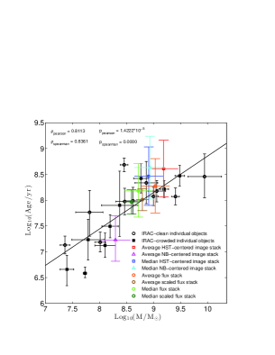
(a)

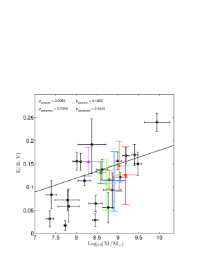
(b)

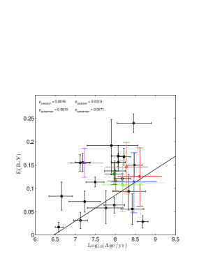
(c)

Figure 5.— These plots show the relationships between (a) stellar mass and age, (b) stellar mass and E(B-V), and (c) age and E(B-V) of the sample. The black points represent the best fitting parameter values for the individual objects, and the remaining color scheme is retained from Figure 3. The error bars plotted are those output by SpeedyMC and are asymmetrical.

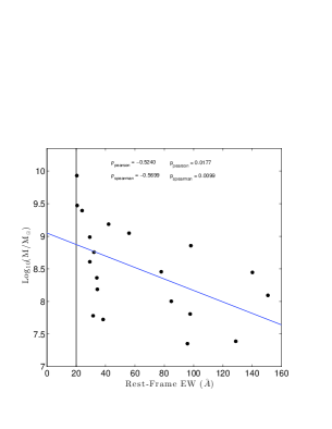
(a)

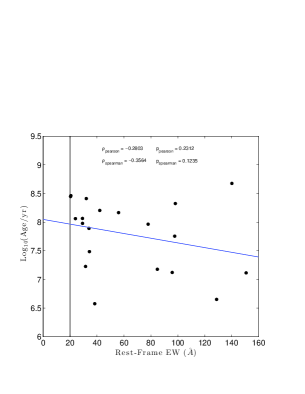
(b)

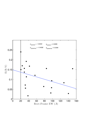
(c)

Figure 6.— These plots show the relationships between (a) stellar mass and Ly$\alpha$ EW, (b) age and Ly$\alpha$ EW, and (c) E(B-V) and Ly$\alpha$ EW of the individual objects.

4.1. Correlations with Equivalent Width

The first panel of Figure 6 shows stellar mass versus the rest-frame Ly$\alpha$ equivalent width (EW). There is a rough upper envelope on the points such that no objects exhibit rest-frame $EW>60$ Angstroms and stellar mass$>10^{9}M_{\odot}$. Because EW was measured via narrow-band $3727\AA$ and broad-band U,B photometry (Guaita et al., 2010), there is no direct selection effect on stellar mass. Hence the lack of high-stellar-mass, high-EW objects implies that galaxies with high stellar mass also have high rest-UV luminosity. This should be reflected via a related dearth of objects with high stellar mass and low SFR i.e. low specific SFRs.

The second panel of Figure 6 shows stellar population ages versus rest-frame EW. Here, one might expect to see a strong correlation, as the Ly$\alpha$ EW of a starburst is a strongly decreasing function of age, and for continuous star formation rate the correlation remains strong (Shapley et al., 2003). The observed lack of correlation implies that Ly$\alpha$ radiative transfer is not trivial; however, it could also be produced by a disconnect between our measured ages and the true age of the starbursting population caused by our assumption of a single stellar population with constant SFR.

The third panel of Figure 6 shows dust reddening, E(B-V), versus rest-frame EW. Though statistically correlated, the correlation is weak. One could expect that dustier galaxies would more effectively quench Ly$\alpha$ photons to produce lower EWs. The lack of strong correlation therefore implies that Ly$\alpha$ radiative transfer is working to prevent Ly$\alpha$ photons from repeated resonant scatters and hence prevents E(B-V) from strongly affecting the resulting Ly$\alpha$ luminosity. This is a particularly interesting point due to the fact that this effect is not seen in other recent LAE studies, but is seen in some local group studies, such as Giavalisco et al. (1996).

(a)

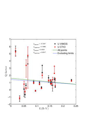
(b)

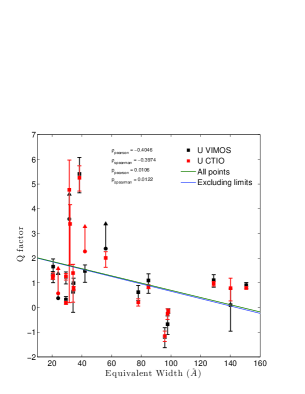
(c)

Figure 7.— These plots show (a) the distribution of Ly$\alpha$ $q$ factors for each of the individual objects, (b) the $q$ factor - E(B-V) relation, and (c) $q$ factor - Ly$\alpha$ EW relation for the individual objects.

4.2. The Ly$\alpha$ q Factor

As mentioned above, we excluded the U-band data from SED-fitting due to this likelihood of Ly$\alpha$ emission making a significant contribution to this broad-band photometry and the impossibility of properly accounting for Ly$\alpha$ radiative transfer in our SED templates. However, this makes the U-band data ideal for an estimation of Ly$\alpha$ $q$ factors, which represent the extent to which Ly$\alpha$ emission from a galaxy has been enhanced ($q>1$) or quenched ($q<1$) along the line-of-sight to Earth. As was first done by Finkelstein et al. (2008), we define $q=\tau_{Ly\alpha}/\tau_{\lambda=1216}$, where $\tau_{\lambda}=k_{\lambda}E(B-V)/1.086$ and $k_{\lambda}$ follows a Calzetti et al. (2000) dust attenuation law. The $q$ factor has typically been measured from the same narrow-band imaging used to select LAEs, leading to a selection against low values of $q$. The deep U-band data in the CANDELS catalog allows us to make a measurement of $q$ from broad-band imaging sensitive to Ly$\alpha$ that is uncorrelated with the original selection of the LAE sample. A $q$ factor of unity implies that Ly$\alpha$ photons see the same dust column as UV continuum photons, whereas a $q$ factor of zero points to Ly$\alpha$ photons seeing no dust extinction whatsoever. A negative $q$ factor would imply Ly$\alpha$ enhancement by a top-heavy IMF, clumpy dust, or anisotropic radiative transfer.

Panel (a) of Figure 7 shows that most objects have $q$ factors between zero and one, as expected. In a few of our objects, noise in the U-band photometry results in very low, even negative, values of $q$. There is no statistically significant correlation with E(B-V) in panel (b), but panel (c) shows a correlation with EW in the expected direction.

4.3. Are LAEs on the SFR-$M_{*}$ “Main Sequence”?

Lastly, in Figure 8, we explore the behavior of the individual object LAEs in the SFR - stellar mass relation. Our individual object LAEs appear to lie systematically above the galaxy main sequence (MS), implying larger star formation rates than expected for galaxies of their mass. Interestingly, the scatter seems to increase toward faint masses. This could happen because a star formation episode of a few $M_{\odot}/yr$ will disturb a lower mass galaxy much more than a higher mass galaxy. In the analysis done in Ibar et al. (2013) and seen in their Figure 8, H$\alpha$ emitters at $z=1.47$ also fall above the Main Sequence, though that study probes much higher masses. One should note that all other studies shown on this plot used the same (Salpeter) IMF, BC03 models, and constant star formation histories as used in this study, ruling out a systematic offset in SFR or $M_{*}$ due to varying assumptions.

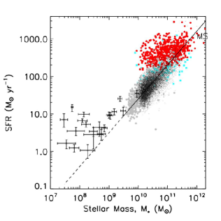
Figure 8.— LAEs at z = 2.1 compared to the galaxy main sequence. Star Formation Rate (SFR) vs. stellar mass (M_∗) for the LAE sample are shown as black points, with error bars. For comparison, the SFR-M_∗ relation at $1.5<z<2.5$ (galaxy main sequence, MS) is illustrated as the solid, black line (Daddi et al. 2007). Individual galaxy measurements reported in Rodighiero et al. (2011) are also shown: Herschel-PACS data for the COSMOS field (red circles) and GOODS-S (cyan squares), BzK-GOODS galaxies (black circles) and BzK-COSMOS galaxies (black points).

4.4. Stacking Results

In order to better discuss how well the individual object SED fitting parameters agree with that of the various stacking techniques, three rows were added to Table 1, containing the average, median, and $1-\sigma$ scatter of the individual object parameters. For simplicity, we define the failure of a stacking technique in a particular parameter to be when the average (median) of the individual results resides outside of the stacked parameter’s error region. Using this definition, the median HST image stack fails in stellar mass, the average NB image stack fails in all three parameters, and the median NB image stack fails in stellar mass. The average flux stack, median flux stack, and average HST image stack match the individual object results in all three SED fitting parameters. It should be stressed that we do not make direct comparisons between median stacks and average parameter values (or vice versa). The spread of individual object and stacked parameters can be seen in Figure 5. While it is not entirely surprising that the NB-centered image stacks perform less well than the HST- centered image stacks, failure of any HST-centered stacking results is striking, since stacking using the CANDELS established positions for the individual objects is a best-case scenario for stacking accuracy. Lower precision position estimates would provide a substantial amount of error in any stacking analysis. It is possible that this discrepancy in the median image stack could be due to a majority of objects receiving contaminating flux from nearby objects in the IRAC infrared bands.

Table 1

CANDELS ID	M∗ ($10^{9}$ M/M⊙)	Age (Gyr)	E(B-V)	best fit $\chi^{2}$/d.o.f
205 (Clean)	$2.474^{+0.328}_{-0.446}$	$0.115^{+0.032}_{-0.035}$	$0.169^{+0.014}_{-0.012}$	81.9/8
991 (Clean)	$0.407^{+0.353}_{-0.118}$	$0.095^{+0.259}_{-0.041}$	$0.137^{+0.018}_{-0.060}$	18.2/8
7097 (Clean)	$0.971^{+0.250}_{-0.158}$	$0.116^{+0.070}_{-0.032}$	$0.156^{+0.013}_{-0.022}$	111.3/8
9125 (Clean)	$0.280^{+0.052}_{-0.176}$	$0.473^{+0.138}_{-0.394}$	$0.029^{+0.059}_{-0.011}$	20.1/8
10220 (Clean)	$0.717^{+0.154}_{-0.164}$	$0.211^{+0.100}_{-0.083}$	$0.094^{+0.020}_{-0.019}$	151.0/8
11824 (Clean)	$0.023^{+0.050}_{-0.005}$	$0.013^{+0.052}_{-0.004}$	$0.031^{+0.022}_{-0.018}$	14.0/8
12369 (Clean)	$0.064^{+0.030}_{-0.020}$	$0.057^{+0.051}_{-0.024}$	$0.058^{+0.013}_{-0.022}$	13.4/8
14889 (Clean)	$0.101^{+0.078}_{-0.016}$	$0.015^{+0.017}_{-0.003}$	$0.156^{+0.011}_{-0.010}$	13.8/8
17254 (Clean)	$8.518^{+2.021}_{-0.893}$	$0.280^{+0.182}_{-0.063}$	$0.240^{+0.016}_{-0.029}$	189.3/8
22689 (Clean)	$0.286^{+0.118}_{-0.073}$	$0.092^{+0.093}_{-0.036}$	$0.064^{+0.015}_{-0.029}$	5.0/8
24168 (Clean)	$1.116^{+0.229}_{-0.219}$	$0.147^{+0.070}_{-0.051}$	$0.121^{+0.019}_{-0.019}$	61.0/8
2210	$1.533^{+0.289}_{-0.281}$	$0.160^{+0.069}_{-0.052}$	$0.168^{+0.018}_{-0.019}$	28.0/8
3826	$0.024^{+0.014}_{-0.003}$	$0.004^{+0.004}_{-0.002}$	$0.083^{+0.034}_{-0.026}$	4.2/8
6696	$0.231^{+0.415}_{-0.095}$	$0.078^{+0.581}_{-0.042}$	$0.192^{+0.025}_{-0.094}$	11.3/8
7408	$0.053^{+0.006}_{-0.002}$	$0.004^{+0.001}_{-0.001}$	$0.017^{+0.011}_{-0.010}$	40.4/8
11292	$0.154^{+0.080}_{-0.038}$	$0.031^{+0.027}_{-0.010}$	$0.113^{+0.007}_{-0.014}$	14.1/8
18836	$0.124^{+0.089}_{-0.035}$	$0.013^{+0.013}_{-0.004}$	$0.155^{+0.017}_{-0.019}$	24.0/8
21026	$0.060^{+0.086}_{-0.023}$	$0.017^{+0.041}_{-0.007}$	$0.072^{+0.016}_{-0.029}$	4.9/8
21553	$0.572^{+0.184}_{-0.169}$	$0.258^{+0.203}_{-0.134}$	$0.056^{+0.035}_{-0.031}$	6.1/8
25902	$2.966^{+0.807}_{-0.454}$	$0.290^{+0.212}_{-0.090}$	$0.150^{+0.020}_{-0.030}$	94.0/8
Average of Individual Results	1.03	0.123	0.113
Median of Individual Results	0.283	0.094	0.117
Scatter of Individual Results	1.896	0.121	0.059
Average Flux Stack	$1.050^{+0.796}_{-0.487}$	$0.184^{+0.471}_{-0.126}$	$0.146^{+0.042}_{-0.066}$	3.6/8
Median Flux Stack	$0.511^{+0.347}_{-0.237}$	$0.148^{+0.335}_{-0.104}$	$0.108^{+0.048}_{-0.062}$	1.7/8
Average HST Image Stack	$1.192^{+1.262}_{-0.448}$	$0.309^{+0.873}_{-0.214}$	$0.124^{+0.066}_{-0.059}$	22.5/8
Median HST Image Stack	$0.810^{+0.451}_{-0.428}$	$0.305^{+0.509}_{-0.245}$	$0.108^{+0.075}_{-0.053}$	11.8/8
Average NB Image Stack	$0.222^{+0.180}_{-0.106}$	$0.018^{+0.044}_{-0.010}$	$0.165^{+0.006}_{-0.057}$	43.5/8
Median NB Image Stack	$0.828^{+0.396}_{-0.489}$	$0.462^{+0.559}_{-0.401}$	$0.101^{+0.103}_{-0.042}$	16.9/8
Scaled Average Flux Stack	$0.525^{+0.280}_{-0.043}$	$0.084^{+0.093}_{-0.017}$	$0.105^{+0.025}_{-0.014}$	48.2/8
Scaled Median Flux Stack	$0.382^{+0.165}_{-0.074}$	$0.091^{+0.096}_{-0.028}$	$0.131^{+0.013}_{-0.030}$	3.31/8
Clean Average Flux Stack	$1.314^{+1.124}_{-0.753}$	$0.206^{+0.635}_{-0.163}$	$0.160^{+0.057}_{-0.076}$	4.6/8
Clean Median Flux Stack	$0.639^{+0.182}_{-0.526}$	$0.348^{+0.098}_{-0.331}$	$0.048^{+0.104}_{-0.016}$	3.7/8
Clean Average HST Image Stack	$0.088^{+0.140}_{-0.031}$	$0.008^{+0.035}_{-0.004}$	$0.140^{+0.028}_{-0.069}$	20.9/8
Clean Median HST Image Stack	$0.049^{+0.309}_{-0.009}$	$0.009^{+0.177}_{-0.004}$	$0.089^{+0.062}_{-0.058}$	23.2/8
Clean Average NB Image Stack	$0.095^{+0.126}_{-0.035}$	$0.007^{+0.029}_{-0.004}$	$0.150^{+0.023}_{-0.072}$	15.8/8
Clean Median NB Image Stack	$0.079^{+0.214}_{-0.049}$	$0.016^{+0.170}_{-0.012}$	$0.131^{+0.042}_{-0.098}$	10.4/8

The average NB image stack is poor at estimating the average parameters for the sample, but other stacking techniques are relatively reasonable. While the error bars for the stacks shown in Figure 3 include sample variance, the large dispersion of properties is still not captured by any stacking method. As can be seen in Table 1 and Figure 5, there is a large dispersion in the values of mass, age and E(B-V) measured from individual objects, and this dispersion is far larger than the measurement uncertainties. As typically implemented, the stacking approach misses this dispersion, and this is a significant weakness versus fitting individual object SEDs. In circumstances where stacking must be used, however, there are statistical methods that can be used to infer the scatter in properties within the population. An upper limit to the uncertainty in the parameters inferred for the stacked population can be obtained by assuming that the dispersion in properties of the underlying population is much larger than the photometric errors (although one should then interpret a median stack carefully because there may not exist a ”typical object”). In this case, the scatter in the parameters for a population of $N$ objects could be quantified as $\sqrt{N}$ times the uncertainty found for their average-stacked SED; this effectively turns the standard deviation of the average back into the standard deviation of the population. We do find that the sample variance found during our bootstrap resampling dominates the flux uncertainties on the stacked SED in most wavebands. However, applying this method to the average flux stack values in Figure 1 would significantly overestimate the observed scatter in individual object properties. A more sophisticated approach would be to use jacknife techniques (Lupton, 1993) where stacks are made from each set of $N-1$ galaxies and the resulting variance in best-fit parameters is turned into an estimate of the scatter of the population.

4.5. Scaled Flux Stacks

While straightforward calculations of average (median) stacks have been standard in the literature, it is also possible to scale all input fluxes (or images) to a common brightness e.g., in H-band, before stacking. This eliminates the influence of variation in overall brightness and focuses the stacking on determining an average (median) SED shape. To test the efficacy of this approach, we introduce scaled average and scaled median flux stacks. The scaled average (median) flux stack was created by determining the average (median) H-band flux and then multiplying each individual input SED and its uncertainties by the factor needed to match that value. As with other stacks, we include uncertainties due to sample variance by following the identical procedure in bootstrap simulations. By their definition, these new scaled average (median) stacked SEDs have the same average (median) as the corresponding flux-stacked SEDs. Their shapes turn out to be similar. Nonetheless, there is significantly less variance among the bootstrap samples due to having removed the impact of brightness variations, and the scaled flux stacks have significantly smaller uncertainties as a result. In Figure 5, we see that these scaled flux stacks perform quite well in tracing the properties of the sample, at least as well as the simple flux-stacked SEDs but with significantly reduced parameter uncertainties due to the reduced uncertainties in the SED. We conclude that scaling is a superior method for producing stacked SEDs and recommend its use in future studies.

4.6. Clean Stacks

As briefly discussed above, in an attempt to test whether or not IRAC contamination could be a strong source of error, we compiled an additional set of stacks using only the ten individual objects whose CANDELS images were free of nearby sources of flux. This was determined by a visual inspection of the photometric images of each object. If an object’s image contained nearby extraneous sources it was not included in these “clean” stacks. Our parallel analysis with these clean stacks produced results similar to the original stacks. So, there is no evidence that IRAC contamination can account for the discrepancies of our results. However, the clean stack analysis lowers the sample size of an already sparse set of objects, so our clean stacking analysis might suffer from significant information loss. Clean stack results are included in Table 1.

The amount gained in a clean versus crowded analysis is questionable. Figure 2 shows the average and median stacked images for the entire sample and the clean sample. Inspection of the rightmost panel shows that a clean sample of 10 objects produces a less reliable median. Rather than excluding crowded regions, the CANDELS catalog photometry used to create our flux stacks utilizes TFIT (Laidler et al., 2007), which seems to perform better than careful qualitative crowdedness assessments by eye. This could cause the flux stacks to be more accurate than image stacks.

5. Discussion & Conclusions

Stacking techniques have been employed for studying low signal to noise objects. However, some stacking methods may be more accurate at modeling the parameters of a sample than others. Through fitting individual SEDs of 20 LAEs at redshift 2.1 individually, and then fitting 6 types of stacked SEDs comprised of the same 20 objects, we have tested the validity of these methods. We find that median flux stacking and average HST-centered image stacking techniques correctly represent the age and stellar mass of a sample, while the median HST-centered image stack performs less adequately. This is a stark result, since our analysis serves as a best-case scenario for stacking. Stacking objects with CANDELS defined coordinates maximizes the accuracy of our stacking sample. We further investigated this result by establishing a set of clean stacks, which are comprised of objects free of nearby sources of flux, and with simulations. The clean stacking analysis sheds little light on the underlying reason for the discrepancies in image-stacked parameter estimates of a sample of individual objects. Future stacking analyses should be wary of disparities in analyses due to errors possibly brought on by the stacking method itself. The simulations show that median image stack photometry is biased considerably low when centroiding errors are significant compared to the PSF. Though this effect is not, in practice, catastrophic for either the NB or HST- centered image stacks, it provides a note of caution. We caution the reader of inconsistencies any stacking analysis may bring forth, and recommend the use of a scaled stacking method where stacking is absolutely necessary.

Our main conclusions are the following:

• A lack of correlation between Ly$\alpha$ EW and age implies either complicated radiative transfer mechanisms, or an inappropriate assumption of a constant SFR in a starbursting sample.

• The narrow distribution of $q$ values peaking near one and lack of correlation between $q$, and E(B-V) implies that radiative transfer mechanisms seem to be working to prevent Ly$\alpha$ photons from resonantly scattering in dusty regions.

• Our sample of LAEs lies systematically above the SFR-stellar mass relation galaxy “main sequence” and shows an increase in scatter above this relation at low mass. This may be caused by ongoing starbursts in these galaxies causing a greater excursion in their specific star formation rates.

• Though some types of stacking represent the average and median properties of a sample well, the large dispersion of individual object properties is obscured by stacking. We recommend a new approach using an H-band scaled median or average flux stack, which reduces uncertainties significantly.

References

- Acquaviva et al. (2011) Acquaviva, V., Gawiser, E., & Guaita, L. 2011, ApJ, 737, 47
- Acquaviva et al. (2012a) Acquaviva, V., Gawiser, E., & Guaita, L. 2012a, in IAU Symposium, Vol. 284, IAU Symposium, ed. R. J. Tuffs & C. C. Popescu, 42–45
- Acquaviva et al. (2012b) Acquaviva, V., Vargas, C., Gawiser, E., & Guaita, L. 2012b, ApJ, 751, L26
- Ashby et al. (2013) Ashby, M. L. N., Willner, S. P., Fazio, G. G., et al. 2013, ApJ, 769, 80
- Bertin & Arnouts (1996) Bertin, E., & Arnouts, S. 1996, A&AS, 117, 393
- Bond et al. (2012) Bond, N. A., Gawiser, E., Guaita, L., et al. 2012, ApJ, 753, 95
- Bruzual & Charlot (2003) Bruzual, G., & Charlot, S. 2003, MNRAS, 344, 1000
- Calzetti et al. (2000) Calzetti, D., Armus, L., Bohlin, R. C., et al. 2000, ApJ, 533, 682
- Calzetti et al. (1994) Calzetti, D., Kinney, A. L., & Storchi-Bergmann, T. 1994, ApJ, 429, 582
- Cowie & Hu (1998) Cowie, L. L., & Hu, E. M. 1998, AJ, 115, 1319
- Dickinson et al. (2003) Dickinson, M., Giavalisco, M., & The Goods Team. 2003, in The Mass of Galaxies at Low and High Redshift, 324
- Fazio et al. (2004) Fazio, G. G., Hora, J. L., Allen, L. E., et al. 2004, ApJS, 154, 10
- Finkelstein et al. (2011a) Finkelstein, S. L., Cohen, S. H., Moustakas, J., et al. 2011a, ApJ, 733, 117
- Finkelstein et al. (2010) Finkelstein, S. L., Papovich, C., Giavalisco, M., et al. 2010, ApJ, 719, 1250
- Finkelstein et al. (2009) Finkelstein, S. L., Rhoads, J. E., Malhotra, S., & Grogin, N. 2009, ApJ, 691, 465
- Finkelstein et al. (2008) Finkelstein, S. L., Rhoads, J. E., Malhotra, S., Grogin, N., & Wang, J. 2008, ApJ, 678, 655
- Finkelstein et al. (2007) Finkelstein, S. L., Rhoads, J. E., Malhotra, S., Pirzkal, N., & Wang, J. 2007, ApJ, 660, 1023
- Finkelstein et al. (2011b) Finkelstein, S. L., Hill, G. J., Gebhardt, K., et al. 2011b, ApJ, 729, 140
- Gawiser et al. (2006a) Gawiser, E., et al. 2006a, ApJ, 642, L13
- Gawiser et al. (2006b) —. 2006b, ApJS, 162, 1
- Gawiser et al. (2007) —. 2007, ApJ, 671, 278
- Giavalisco et al. (1996) Giavalisco, M., Koratkar, A., & Calzetti, D. 1996, ApJ, 466, 831
- Giavalisco et al. (2004) Giavalisco, M., et al. 2004, ApJ, 600, L93
- Guaita et al. (2010) Guaita, L., Gawiser, E., Padilla, N., et al. 2010, ApJ, 714, 255
- Guaita et al. (2011) Guaita, L., Acquaviva, V., Padilla, N., et al. 2011, ApJ, 733, 114
- Guo et al. (2013) Guo, Y., Ferguson, H. C., Giavalisco, M., et al. 2013, ApJS, 207, 24
- Hagen, A., et al. (2013, in prep.) Hagen, A., et al. 2013, in prep.
- Ibar et al. (2013) Ibar, E., Sobral, D., Best, P. N., et al. 2013, ArXiv e-prints, arXiv:1307.3556
- Koekemoer et al. (2011) Koekemoer, A. M., Faber, S. M., Ferguson, H. C., et al. 2011, ApJS, 197, 36
- Koekemoer et al. (2012) Koekemoer, A. M., Ellis, R. S., McLure, R. J., et al. 2012, ArXiv e-prints, arXiv:1212.1448
- Kriek et al. (2010) Kriek, M., Labbé, I., Conroy, C., et al. 2010, ApJ, 722, L64
- Lai et al. (2008) Lai, K., et al. 2008, ApJ, 674, 70
- Laidler et al. (2007) Laidler, V. G., Papovich, C., Grogin, N. A., et al. 2007, PASP, 119, 1325
- Lewis & Bridle (2002) Lewis, A., & Bridle, S. 2002, Phys. Rev. D, 66, 103511
- Lupton (1993) Lupton, R. 1993, Statistics in Theory and Practice (Princeton University Press)
- Madau (1995) Madau, P. 1995, ApJ, 441, 18
- Meidt et al. (2013) Meidt, S., Schinnerer, E., Hughes, A., et al. 2013, in American Astronomical Society Meeting Abstracts, Vol. 221, American Astronomical Society Meeting Abstracts, 349.17
- Nilsson et al. (2011) Nilsson, K. K., Östlin, G., Møller, P., et al. 2011, A&A, 529, A9
- Nilsson et al. (2007) Nilsson, K. K., et al. 2007, A&A, 471, 71
- Ono et al. (2010a) Ono, Y., Ouchi, M., Shimasaku, K., et al. 2010a, ApJ, 724, 1524
- Ono et al. (2010b) —. 2010b, MNRAS, 402, 1580
- Ouchi et al. (2010) Ouchi, M., Shimasaku, K., Furusawa, H., et al. 2010, ApJ, 723, 869
- Pentericci et al. (2008) Pentericci, L., Grazian, A., Fontana, A., et al. 2008, A&A, in press, arXiv:0811.1861, arXiv:0811.1861
- Pirzkal et al. (2007) Pirzkal, N., Malhotra, S., Rhoads, J. E., & Xu, C. 2007, ApJ, 667, 49
- Rhoads et al. (2000) Rhoads, J. E., Malhotra, S., Dey, A., et al. 2000, ApJ, 545, L85
- Shapley et al. (2003) Shapley, A. E., Steidel, C. C., Pettini, M., & Adelberger, K. L. 2003, ApJ, 588, 65
- Windhorst et al. (2011) Windhorst, R. A., Cohen, S. H., Hathi, N. P., et al. 2011, ApJS, 193, 27
- Zibetti et al. (2013) Zibetti, S., Gallazzi, A., Charlot, S., Pierini, D., & Pasquali, A. 2013, MNRAS, 428, 1479