Propagation of Phonons in a Curved Space Induced by Strain Fields Instantons

Abstract

We show that for a multiple-connected space the low energy strain fields excitations are given by instantons. Dirac fermions with a chiral mass and a pairing field propagates effectively in a multiple conected space. When the elastic strain field response is probed one finds that it is given by the Pointriagin characteristic. As a result the space time metric is modified. Applying an external stress field we observe that the phonon path bends in the transverse direction to the initial direction.

I- Introduction

Gauge theories and their applications to gravity and elasticity are important tools in modern physics Kleinert ; Kleinertnew . In gauge theories the gauge potential is fundamental and determines the field strength. The same approach is used in gravity where the vierbein (the transformation matrix of the coordinates ) determines the spin-connection and the curvature Nieh ; Kleinert . The similarity between the theory of gravity and elasticity has been pointed out by Kleinert Kleinert . The classical theory of elasticity Lifshitz is based on the formalism of coordinates transformations between the perfect and the deformed crystal. As a result the space derrivatives are replaced by covariant derivatives which introduce the concept of spin-connection. The disclinations density have been described by the spatial part of the Einstein tensor and the dislocation density are given by the torsion tensor Katanev ; Kleinert . The spin-connection might play a the same fundamental role in elasticity as the gauge fields in gauge theories. This suggests the possibility of instantons in elasticity. This possibility follows from Volterra’s work Volterra , which used the homotopy method to describe disclinations and dislocations . The Saint Venat compatibility conditions imply that the torsion and curvature must vanish Volterra ; Kleinert . Volterra concluded that the equilibrium state of a simply connected elastic body is a state with zero strain, while the equilibrium state of a multiple-connected one could have non-vanishing kinetic energy with non-vanishing strain Delphenich . Such a state corresponds to the existence of quantum instantons, similar to the metastable states for two dimensional isotropic ferromagnet and four dimensional Yang-Mills fields Yang-Mills . In order to realize the physics of instantons in elasticity, one needs a multiple-connected space. For example when the Dirac Hamiltonian contains a chiral mass $\gamma_{5}m$, the model will have zero modes and therefore is topological non-trivial. If instead of probing the Dirac Hamiltonian with an external electromagnetic field one probes the system with a strain field the response will generates the Pointriagin characteristic Nakahara . This response is similar to the one in electromagnetism where the Dirac Hamiltonian with a chiral mass $\gamma_{5}m$ modifies the Maxwell’s equation by the term $\delta H\propto\theta\vec{E}\cdot\vec{B}$ ( $\theta$ represents the axion field Wilczek ). Such a term gives rise to the Faraday and Kerr rotation Karch ; Tse ; Obukhov ; davidM .

Inspired by the analogy between the gauge theory and the theory of elasticity Kleinert ; Nieh we expect an elastic analog to the magnetoelectic effect. In elasticity the phonon replaces the photon therefore, an analog to the Farady effect is expected. This suggests that a medium which is described by an elastic topological invariant will affect the phonon propagation and polarization. In elasticity a local crystal deformation induces a spin-connection which has curvature (disclinations) and an elastic Pointriagin invariant. For a Dirac Hamiltonian with a chiral mass term $\gamma_{5}m$ and a pairing field one obtains a topological superconductor. For such a case we can use the elastic response to identify the topological superconductor. The topological invariants in elasticity are given by their analog in gravity, the Pointriagin and the Euler characteristic (see eqs.$(3,4)$ in ref.Yang-Mills ). For the Yang-Mills gauge theory YGGR the Pointriagin electromagnetic characteristics YGGR are known to give rise to the Yang-Mills instantons excitations.

In the continuum theory of elasticity the equilibrium position of the atoms in a solid Lifshitz is given by the coordinate $\vec{r}$ . A small crystal perturbation is described by the elastic field $u^{a}(\vec{r},t)$ ($a=1,2,3$ represents the Cartesian coordinates). Due to the periodicity of the elastic field, the deviation from equilibrium $u^{a}(\vec{r},t)$ and $u^{a}(\vec{r}+\vec{a},t)$ describes the same physical excitation ($\vec{a}$ represents the crystal Bravais lattice) Kleinert . Due to the presence of the electron lattice coupling one expects that the lattice strain field $u^{a}(\vec{r},t)$ defined in the absence of superconductivity will be modified once superconductivity is switched on . As a result the coordinate $\vec{r}$ must be replaced by a new lattice coordinate, $\vec{r}\rightarrow\vec{r}+\vec{e}(\vec{r},t)$. When the lattice coordinates are modified the displacement field $u^{a}(\vec{r},t)$ is replaced by the field $u^{a}(\vec{e}(\vec{r},t))$ which induces new strain fields. Following ref. Nieh ; Kleinert the derivatives with respect the Lorentz coordinates $\mu=t,x,y,z$ Kleinert are replaced by the covariant derivative $\nabla_{\mu}$ with the spin-connection $A^{a,b}=A^{a,b}_{\mu}dx^{\mu}$. The covariant derivative of the elastic field $u^{a}(\vec{r},t)$ and the electronic spinor $\Psi$ are given by : $\nabla_{\mu}u^{a}(\vec{r},t)=\partial_{\mu}u^{a}(\vec{r},t)+A^{a,b}_{\mu}u^{b}(\vec{r},t)$ and $\nabla_{\mu}\Psi(\vec{r},t)=\partial_{\mu}\Psi(\vec{r},t)+\frac{1}{4}A_{\mu}^{a,b}[\gamma^{a},\gamma^{b}]\Psi$ where $a=0,1,2,3$ and $\gamma^{a}$ are the Dirac matrices .

The integration of the Dirac fermion in the presence of the term $\gamma_{5}m$ induces the Pointriagin characteristic Richter ; Egouchi ; Freund $\int d^{4}x\sqrt{-g}[\frac{1}{768\pi^{2}}\epsilon^{\mu,\nu,\alpha,\beta}F^{a}_{\alpha,\beta,b}F^{a}_{\mu,\nu,b}]$ given in terms of the metric tensor $g_{\mu,\nu}$ and elastic field strength $F_{\mu,\nu,b}^{a}=\partial_{\mu}A_{\nu}^{a,b}-\partial_{\nu}A_{\mu}^{a,b}+[A_{\mu},A_{\mu}]^{a}_{b}$. From the work of Katanev we learn that the elastic deformations which describe the topological defects is given by a term which is similar to the Hilbert-Einstein action (see eq.$(30)$ in ref. Katanev . The variation of the elastic action is satisfied for elastic field strengths which satisfy the duality or anti-duality conditions $\tilde{A}^{a,b}=\pm A^{a,b}$ From the analogy with the Yang-Mills gauge fields we learn that the instanton field obeys the duality or anti-duality conditions $\tilde{F}_{\mu,\nu}^{a,b}=\pm F_{\mu,\nu}^{a,b}$ , $\tilde{F}_{\mu,\nu,b}^{a,b}\equiv\frac{1}{2}\sum_{c=0,d=0}^{c=3,d=3}\epsilon_{abcd}F_{\mu,\nu}^{c,d}$. Each solution is satisfied for an arbitrary integration constant $\Lambda$. For each $\Lambda$ the Pointriagin action gives the instanton weight, $e^{-\frac{\Lambda^{2}}{const}}$ in agreement Egouchi ; Freund .( As a result the metric satisfy at long distances the conditions $g_{\mu,\nu}\rightarrow 0$ with the field strength $F^{\alpha}_{\beta,\mu,\nu}$ and the Ricci curvature $F_{\mu,\nu}$ obey:$F^{\alpha}_{\beta,\mu,\nu}\rightarrow 0$ , $F_{\mu,\nu}\rightarrow 0$ . Only the scalar curvature $g^{\mu,\mu}F_{\mu,\mu}$ is finite Egouchi .)

The purpose of this paper is to investigate the propagation of the phonon field in a space controlled by the metric tensor $g_{\mu,\nu}$ induced by the instantons. Using the Euclidean version sound of the Lorentz transformation we describe the unperturbed crystal which as $S^{3}$ Euclidean space. The effective action of the crystal is given by the elasticity action Katanev ; Kleinert which is similar to the gravitation Einstein action. A topological superconductor for a Dirac Hamiltonian with pairing interaction which is controlled by the crystal deformation, the presence of a term of the form $\gamma_{5}$ coupled to the order parameter of the Superconductor Superconductor gives rise to the Pointriagin action. controlled by the saddle point of the Superconducting order parameter. (The elastic deformed crystal affects the electronic action by generating an elastic term which given by the Pointriagin characteristic in elasticity Richter ; YGGR ). The possible elastic deformation of the Euclidean $S^{3}$ sphere which obey the elastic version of the Hilbert-Einstein action Katanev satisfies the duality or anti-duality relations. Each deformation of the crystal corresponds to a metric solution with a different integration factors $\Lambda$. For each $\Lambda$ we have an instanton contribution to the action $e^{-\frac{\Lambda^{2}}{const}}$. The maximum contribution to the action comes from the unperturbed crystal with $\Lambda=0$. The propagation of the phonon is affected by the metric tensor. For each value $\Lambda$ we have a different metric which will affect the phonon propagation. Therefore the phonon propagation is obtained after we add all the contributions. In order to enhance the statistical weight for values of $\Lambda\neq 0$ we can bend the crystal in the superconducting phase. As a concrete example we compute the metric tensor for a fixed value of $\Lambda$ . Using the computed metric tensor we compute numerically the propagation of the phonon at long distances and find a bended path .

The plan of this paper is as follows. In Sec. $II$ we introduce the Pointriagin index in gravity and propose that such an index emerges also in elasticity under certain conditions. Sec.$III$ presents the emergence of the Pointriagin index in elasticity. In addition the elastic energy of the crystal gives rise to a term similar to the Einstein curvature or density. In Sec.$IV$ we show that the Green’s function of the lattice is a function of the metric. Therefore the propagation of the elastic waves is obtained after performing a statistical average over the metric. Sec.$V$ is devoted to computation of the metrics. The spin connection needs to satisfy self duality conditions. As a result one find that at long distance a metric characterized by the integration factor $\Lambda$. In Sec.$VI$ we consider a simplified version of the problem and show that for a single value of $\Lambda\neq 0$ we obtain at long distances a bended path for the propagating phonon.

II-The Pointriagin index in electromagnetism and gravity

The Pointriagin index $\nu$ measures the difference between the vanishing eigenvalues of positive and negative chirality of the Euclidean Dirac operator $\gamma^{\mu}D_{\mu}[\vec{A}]$ (in the presence of the electromagnetic field $\vec{A}$) with eigenvalues $\gamma_{5}=\pm 1$ Nakahara .

$$I_{P}=\nu\equiv n_{+}-n_{-}=\frac{1}{16\pi^{2}}\int d^{4}xTr[\tilde{F}_{\mu,\nu}F^{\mu,\nu}]=-\frac{1}{14\pi^{2}}\int d^{4}x[\vec{E}\cdot\vec{B}]$$ (1)

$\tilde{F}_{\mu,\nu}$ is the dual strength field ($\vec{B}$) of $F^{\mu,\nu}$ (the field $\vec{E}$). The Pointriagin index has been defined in gravity Egouchi ; Richter and also used for Topological Superconductors Ludwig ; Wang where $A^{a,b}_{\mu}$ is the spin- connection .

$$I_{p,el.}=\nu\equiv n_{+}-n_{-}=-\int d^{4}x\sqrt{-g}[\frac{1}{768\pi^{2}}\epsilon^{\mu,\nu,\alpha,\beta}F^{a}_{\alpha,\beta,b}F^{a}_{\mu,\nu,b}];\hskip 7.22743ptg\equiv det[g_{\mu,\nu}]$$ (2)

We will show in the next section that the effect of strain fields in elasticity coupled to a pairing field generates a Pointriagin term as encountered in gravity. Katanev . In a crystal the presence of an external stress or defects such as dislocations or disclinations induce a strain field Katanev . The strain field gives rise to a spin-connection $A^{a,b}_{\mu}$ with the elastic field strength $F^{a}_{\alpha,\beta,b}$ Katanev ; Kleinert .

III- Construction of the effective action for a Dirac Hamiltonian with a pairing interaction coupled to elasticity

The Pointriagin index in elasticity is obtained for a Dirac Hamiltonian with a pairing interaction coupled to the crystal strain field in the superconducting phase. The Dirac Hamiltonian Chamon with a paring interaction $\varphi$ and $\varphi^{*}$ is a function crystal field $\vec{u}(\vec{r},t)$.

$$H^{s.c}=\int_{-\infty}^{\infty}\,dt\int d^{3}r\Big{[}[\psi^{\dagger}_{\uparrow}(\vec{r},t),\psi^{\dagger}_{\downarrow}(\vec{r},t)]^{T}(\sigma^{1}(-i)\partial_{1}+\sigma^{2}(-i)\partial_{2})[\psi_{\uparrow}(\vec{r},t),\psi_{\downarrow}(\vec{r},t)]$$

$$+\varphi(\vec{r},t)\psi^{\dagger}_{\uparrow}(\vec{r},t)\psi^{\dagger}_{\downarrow}(\vec{r},t)+\varphi^{*}(\vec{r},t)\psi_{\downarrow}(\vec{r},t)\psi_{\uparrow}(\vec{r},t)\Big{]}-\int_{-\infty}^{\infty}dt\int d^{3}r\varphi^{*}(\vec{r},t)\varphi(\vec{r},t)$$

We introduce a four component spinor

$$\Psi\equiv[\psi_{\uparrow},\psi_{\downarrow},\psi^{*}_{\downarrow},-\psi^{*}_{\uparrow}]^{T}$$ (4)

The spinor $\Psi$ obeys : $\Psi_{C}=C\Psi^{*}=\Psi$;     $C=i\sigma^{2}\times\tau_{2}$ where $\sigma^{2}$ is the spin Pauli matrix and $C=i\sigma^{2}\times\tau_{2}$ is charge conjugation matrix. Using the constrained spinor $\Psi=C\Psi^{*}$ we obtain the Dirac Hamiltonian with pairing interaction Chamon .

$$S[\bar{\Psi},\Psi,\varphi,\vec{u}(\vec{r},t)]=\int_{-\infty}^{\infty}dt\int d^{3}r\Big{[}\bar{\Psi}(\vec{r},t)[i\gamma^{0}\partial_{t}+i\gamma^{1}\partial_{1}+i\gamma^{2}\partial_{2}+i\gamma^{3}\partial_{3}+\varphi_{r}+i\gamma^{5}\varphi_{I}]\Psi(\vec{r},t)\Big{]}$$

$$-\frac{1}{2}\int_{-\infty}^{\infty}dt\int d^{3}r(\varphi^{2}_{r}(\vec{r},t)+\varphi^{2}_{I}(\vec{r},t))+\int_{-\infty}^{\infty}dt\int d^{3}r\frac{1}{2}[\partial_{t}(u^{a}(\vec{r},t))^{2}-\lambda_{c,a,d,b}\partial_{c}(u^{a}(\vec{r},t))\partial_{d}(u^{b}(\vec{r},t))]$$

$\varphi_{r}$ and $\varphi_{I}$ are the real and imaginary pairing field. We have included in eq.$(5)$ ( the last term) the crystal action in the $harmonic$ approximation Lifshitz with the Lame coefficients $\lambda_{\mu,a,\nu,b}$ Lifshitz , $\lambda_{c,a,d,b}=(K-\frac{2}{3}\mu)\delta_{c,a}\delta_{d,b}+G(\delta_{c,d}\delta_{a,b}+\delta_{c,b}\delta_{a,d})$. $K$ is the compressibility and $\mu$ is the shear modulus of the crystal. When the pairing field vanish $\varphi=0$, $\varphi^{*}=0$ the Green’s function for the lattice field $u^{a}(\vec{r},t)$ is given by: $G^{a,b}(\vec{r},\vec{r^{\prime}};t-t^{\prime})=-i\langle 0|T\Big{[}u^{a}(\vec{r},t)u^{b}(\vec{r^{\prime}},t^{\prime})\Big{]}|0\rangle$. Where $|0\rangle$ is the unperturbed crystal and $T$ is the time order operator Kleinert . When $\varphi=\varphi^{*}=0$ the crystal is described by the coordinate $t$ and $\vec{r}$ which satisfy the sound Lorentz transformation, $ds^{2}=-c^{2}dt^{2}+dx^{2}+dy^{2}+dz^{2}$, $c=1$ is the speed of sound (transversal or longitudinal). In the superconducting phase the pairing fields $\varphi\equiv\varphi(\vec{u}(\vec{r},t))$ , $\varphi^{*}(\vec{u}(\vec{r},t))$ generates the mass term $\gamma_{5}m$ ($m\equiv<\varphi_{r}>=<\varphi+\varphi^{*}>$) responsible for the Pointriagin term. These terms are function of the crystal strain field $u^{a}(\vec{r},t)$ and the external stress . In particular when external defects such as dislocations or disclination Kleinert ; Katanev ; davidNJP are introduced in the superconducting phase the new coordinates will be given by $\vec{W}(\vec{r},t)$. The deformed coordinates induced by the elastic deformations obeys the sound Lorentz transformation, with the new coordinates $[t^{\prime}(\vec{r},t),\vec{W}(\vec{r},t)]\equiv[t^{\prime}(\vec{r},t),\vec{r}+\vec{e}(\vec{r},t)]$. This transformation replaces crystal displacement field $\vec{u}(\vec{r},t)$ by $\vec{u}(\vec{W}(\vec{r},t))$.

Following Cartan formalism Nieh we incorporate the coordinate transformations with the help of the vierbein matrix $e^{a}_{\mu}(\vec{r},t)\equiv\partial_{\mu}W^{a}(\vec{r},t)$ and the metric tensor $g_{\mu,\nu}$.

$$e^{a}_{\mu}(\vec{r},t)\equiv\partial_{\mu}W^{a}(\vec{r},t);a=0,1,2,3;\mu=t,x,y,z$$

$$g_{\mu,\nu}=\sum_{a=0}^{3}e^{a}_{\mu}e^{a}_{\nu}$$

$$\sum_{\mu}e^{a}_{\mu}e^{\mu}_{b}=\eta_{a,b}$$

$\eta_{a,b}=(-1,1,1,1)$, for the Euclidean case $\eta_{a,b}$ is replaced by $\delta_{a,b}$ Using the matrix $e^{a}_{\mu}$ we describe the transformation from $local$ orthonormal coordinates $a=0,1,2,3$ to the fixed Cartesian frame (given by the Greek letters) $\mu=t,x,y,z$. Following ref. Nieh ; davidNJP we obtain the elastic spin-connection $A^{a,b}_{\mu}$

$$A_{\mu}^{a,b}=\frac{1}{2}[e^{\nu,a}(\partial_{\mu}.e^{b}_{\nu}-\partial_{\nu}e^{b}_{\mu})-e^{\nu,b}(\partial_{\mu}e^{a}_{\nu}-\partial_{\nu}e^{a}_{\mu})-e^{\rho,a}e^{\sigma,a}(\partial_{\rho}e_{\sigma,a}-\partial_{\sigma}e_{\rho,c})e^{c}_{\nu}]$$

$$e^{a,\nu}\equiv e^{a}_{\sigma}g^{\sigma,\nu}$$

The covariant derivative of the spinor $\Psi$ with the four components $\Psi^{a}(\vec{r},t)$, $a=0,2,3,4$ is given by:

$$\nabla_{\mu}\Psi(\vec{r},t)=\partial_{\mu}\Psi(\vec{r},t)+\frac{1}{4}A_{\mu}^{a,b}[\gamma^{a},\gamma^{b}]\Psi$$

where $\gamma^{0}=I\times\tau_{3}$ and $\gamma^{a}=\sigma^{a}\times i\tau_{2}$ for $a=1,2,3$. $\tau$ the denotes the Pauli matrix in the $orbital$ or $chiral$ space and $I$, $\sigma^{a}$ represents the Pauli matrix in the $SU(2)$ spin space . Due to the elastic strain field the derivative of the elastic field $\vec{u}(\vec{r},t)$ is replaced by the covariant derivative $\nabla_{\mu}$ given in terms of the the same spin-connection A${}^{a,b}_{\nu}(\vec{r},t)$ which determine the covariant derivative of the fermion spinor.

$$\nabla_{\mu}u^{a}(\vec{r},t)=\partial_{\mu}u^{a}(\vec{r},t)+A^{a,b}_{\mu}u^{b}(\vec{r},t)$$ (9)

As a result the strength field $F_{\mu,\nu,b}^{a}$ given in terms of the spin-connection $A_{\mu}^{a,b}$.

$$F_{\mu,\nu,b}^{a}=\partial_{\mu}A_{\nu}^{a,b}-\partial_{\nu}A_{\nu}^{a,b}+[A_{\mu},A_{\mu}]^{a}_{b}$$ (10)

The curvature tensor $R_{\mu,\nu}^{\sigma,\tau}$, the Ricci tensor $R_{\mu,\nu}$ and the scalar curvature $R$ are given with the help of the spin-connection $A_{\mu}^{a,b}$ and the vierbein matrix $e^{a}_{\mu}(\vec{r},t)$:

$$R_{\mu,\nu}^{\lambda,\sigma}=e^{\lambda}_{a}e^{\sigma}_{b}F_{\mu,\nu}^{a,b}$$

$$F_{\mu,\nu,b}^{a}=e^{a}_{\sigma}e^{\tau}_{b}R_{\mu,\nu}^{\sigma,\tau}$$

$$R_{\mu,\nu}=R_{\mu,\lambda,\nu}^{\lambda}=e^{\lambda}_{a}e^{b}_{\lambda}F_{\mu,b,\nu}^{a}=\eta^{b}_{a}F_{\mu,b,\nu}^{a}=\epsilon_{\mu\alpha\beta}\epsilon_{\nu\rho\sigma}\partial_{\alpha}\partial_{\beta}\partial_{\rho}W_{\sigma}(\vec{r},t)$$

$$R=g^{\nu,\mu}R_{\nu,\mu}=\eta^{b}_{a}F_{\mu,b,\nu}^{a}$$

The the vierbein will determine the spin-connection the field strength,curvature, Ricci tensor , scalar curvature and the behavior of the fields $\Psi(\vec{r},t)$ and $\vec{u}(\vec{r},t)$.

and they affect the spinor field $\Psi(\vec{r},t)$ and the elastic field $\vec{u}(\vec{r},t)$.

The action for the electrons and lattice in the harmonic representation $S[\bar{\Psi},\Psi,\varphi,\vec{u}]$ will be replaced by the spin-connection and vierbein:

$$S[\bar{\Psi},\Psi,\varphi,\vec{u}]\rightarrow\hat{S}[\bar{\Psi},\Psi,\varphi;e^{a}_{\mu},A^{a,b}_{\mu},\vec{u}]$$ (12)

As a result the partition function will be given by :

$$Z=\int\,D\bar{\Psi}D\Psi D\varphi DuDe^{a}_{\mu}DA^{a,b}_{\mu}e^{i\hat{S}[\bar{\Psi},\Psi,\varphi;e^{a}_{\mu},A^{a,b}_{\nu},\vec{u}]}$$ (13)

The integration measure $De^{a}_{\mu}DA^{a,b}_{\mu}$ described all the possible elastic deformation which can be generated by the configuration $\vec{W}(\vec{r},t)$. The integration measure $Du$ describes the small deviation in the harmonic approximation for different crystal configurations $\vec{W}(\vec{r},t)$. The explicit form of the action for the deformed crystal will be :

$$\hat{S}[\bar{\Psi},\Psi,\varphi;e^{a}_{\mu},A^{a,b}_{\nu},\vec{u}]=\int_{-\infty}^{\infty}dt\int-d^{3}r\sqrt{det[g_{\mu,\nu}]}\Big{[}\bar{\Psi}(\vec{r},t)[i\gamma^{0}e^{\mu}_{0}(\partial_{\mu}+\frac{1}{8}A_{\mu}^{a,b}[\gamma^{a},\gamma^{b}])$$

$$+i\gamma^{1}e^{\mu}_{1}(\partial_{\mu}+\frac{1}{8}A_{\mu}^{a,b}+i\gamma^{2}e^{\mu}_{2}(\partial_{2}+\frac{1}{8}A_{\mu}^{a,b}[\gamma^{a},\gamma^{b}])+i\gamma^{3}e^{\mu}_{3}(\partial_{\mu}+\frac{1}{8}A_{\mu}^{a,b}[\gamma^{a},\gamma^{b}])+\varphi_{r}(\vec{r},t)$$

$$+i\gamma^{5}\varphi_{I}(\vec{r},t)]\Psi(\vec{r},t)\Big{]}-\frac{1}{2}\int_{-\infty}^{\infty}dt\int d^{3}r\sqrt{-det[g_{\mu,\nu}]}(\varphi_{r}^{2}(\vec{r},t)+\varphi_{I}^{2}(\vec{r},t))$$

$$+\int_{-\infty}^{\infty}dt\int d^{3}r\sqrt{-det[g_{\mu,\nu}]}\frac{1}{2}\Big{[}e^{\mu}_{0}\nabla_{\mu}(u^{a}(\vec{r},t))^{2}-\lambda_{c,a,d,b}e^{\mu}_{c}\nabla_{\mu}(u^{a}(\vec{r},t))e^{\nu}_{d}\nabla_{\nu}(u^{b}(\vec{r},t))\Big{]}$$

We perform the chiral transformation and observe that the integration measure is not invariant Fujikawa . We integrate the Dirac Fermions action in the presence of the chiral pairing field $i\gamma^{5}\varphi_{I}(\vec{r},t)$ and compute the sadle point with respect $\varphi_{r}$ davidM and find in agreement with Egouchi ; Richter .

$$\hat{S}_{eff.}[e^{a}_{\mu},A^{a,b}_{\nu},\vec{u}]=\int_{-\infty}^{\infty}\sqrt{-det[g_{\mu,\nu}]}\,dt\int_{-\infty}^{\infty}\,d^{3}r\Big{[}(\frac{\theta}{1536\pi^{2}})\epsilon^{\mu,\nu,\alpha,\beta}F^{a}_{\alpha,\beta,b}F^{a}_{\mu,\nu,b}-\mathbf{E}(g,|\varphi|)\Big{]}$$

$$+\int_{-\infty}^{\infty}\,dt\int_{-\infty}^{\infty}\,d^{3}r\sqrt{-det[g_{\mu,\nu}]}\frac{1}{2}\Big{[}e^{\mu}_{0}\nabla_{\mu}(u^{a}(\vec{r},t))^{2}-\lambda_{c,a,d,b}e^{\mu}_{c}e^{\nu}_{d}\nabla_{\mu}(u^{a}(\vec{r},t))\nabla_{\nu}(u^{b}(\vec{r},t))\Big{]}$$

$$\theta=\frac{1}{2}tan^{-1}(\frac{\varphi_{I}}{\varphi_{r}})$$

The value of the $\theta$ term is determined by the saddle point value for the pairing field $\varphi$ as in ref. davidM . The the first term of the action $\hat{S}_{eff.}$ is proportional to the Pointriagin index $I_{p.el.}$ in eq. $(2)$ . This term gives rise to $instantons$ excitations similar to the one obtained for the Yang Mills action Egouchi ; Yang-Mills ; YGGR . The second term in equation $(16)$ represents the change in the electronic energy due to the the superconductor $\mathbf{E}(g,|\varphi|)\equiv\mathbf{E}(g)-c_{0}\varphi^{2}>0$: $\mathbf{E}(g)$ represents the energy of the free Dirac Hamiltonian in the non-superconducting phase . For the superconducting case the electronic energy is lowered by the pairing energy $-c_{0}\varphi^{2}$. We observe that the spin connection which determines the Pointriagin action (the first term in equation $(16)$ affects also the equation of motion for the elastic field $u^{a}(\vec{r},t)$. The variation of the elastic action with respect the elastic strain field $u^{a}(\vec{r},t)$, $\frac{\delta S_{el.}}{\delta u^{a}(\vec{r},t)}=0$ gives the equation of motion for the sound waves in the deformed space. It is possible to decompose $u^{a}(\vec{r},t)$ into the transversal field $u^{a}_{T}(\vec{r},t)$ and the longitudinal one $u^{a}_{L}(\vec{r},t)$:

$$u^{a}(\vec{r},t)=u^{a}_{T}(\vec{r},t)+u^{a}_{L}(\vec{r},t)$$ (16)

The transversal and longitudinal fields propagate with the sound velocities $c_{T}=\sqrt{\frac{\mu}{\rho}}$ (transversal) and $c_{L}=\sqrt{\frac{\lambda+2\mu}{\rho}}$ (longitudinal) . The effective action for the metric $g_{\mu,\nu}$ is obtained as a result the integration of the field $u^{a}(\vec{r},t)$. For simplicity we will approximate the dynamics of the crystal by two scalar fields $u_{s}(\vec{r},t)$ where $s=T,L$ this will allow to replace the action by a scalar action :

$$\hat{S}_{eff.}[e^{a}_{\mu},A^{a,b}_{\nu},\vec{u}]=\int_{-\infty}^{\infty}\sqrt{-det[g_{\mu,\nu}]}\,dt\int_{-\infty}^{\infty}\,d^{3}r\Big{[}(\frac{\theta}{1536\pi^{2}})\epsilon^{\mu,\nu,\alpha,\beta}F^{a}_{\alpha,\beta,b}F^{a}_{\mu,\nu,b}-\mathbf{E}(g,|\varphi|)\Big{]}$$

$$+\int_{-\infty}^{\infty}\,dt\int_{-\infty}^{\infty}\,d^{3}r\sqrt{-det[g_{\mu,\nu}]}\frac{1}{2}\Big{[}g^{\mu,\nu}\partial_{\mu}u_{s}(\vec{r},t)\partial_{\nu}u_{s}(\vec{r},t)+J_{s}(\vec{r},t)u_{s}(\vec{r},t)\Big{]}$$

$$\theta=\frac{1}{2}tan^{-1}(\frac{\varphi_{I}}{\varphi_{r}})$$

$J_{s}(\vec{r},t)$ is the external current used to compute the Green’s function. Using the scalar approximation we perform the integration over the field $u_{s}(\vec{r},t)$ and find the effective action. The elasticity contribution to the effective action for a scalar field was given in ref. Christensen and more recently in elasticity Katanev . There are two contributions ; $\kappa$ a constant shift in the ground state energy and a term $B(\mu)R$ with $B(\mu)$ being proportional to the shear modulus $\mu$ of the crystal and $R$ the scalar curvature.

$$S_{eff.}[e^{a}_{\mu},A^{a,b}_{\mu};J_{s}]\equiv S_{eff.}[e^{a}_{\mu},A^{a,b}_{\mu}]+\int_{-\infty}^{\infty}\,dt\int d^{3}r\int_{-\infty}^{\infty}\,dt^{\prime}\int d^{3}r^{\prime}\Big{[}J_{s}(\vec{r},t)g_{s}(\vec{r},\vec{r}^{\prime};t-t^{\prime})J_{s}(\vec{r}^{\prime},t^{\prime})\Big{]}$$

$$S_{eff.}[e^{a}_{\mu},A^{a,b}_{\mu}]=\int_{-\infty}^{\infty}\,dt^{\prime}L_{eff.}[e^{a}_{\mu}(\vec{r},t^{\prime}),A^{a,b}_{\mu}(\vec{r},t^{\prime})]$$

$$\approx\int\,dt\int d^{3}r\sqrt{-det[g_{\mu,\nu}]}\Big{[}(\frac{\theta}{1536\pi^{2}})\frac{1}{2}\epsilon^{\mu,\nu,\alpha,\beta}F^{a}_{\alpha,\beta,b}F^{a}_{\mu,\nu,b}+e_{a,\alpha}e^{\alpha}_{b}F^{a,b}_{\mu,\nu}B(\mu)-\kappa_{eff.}\Big{]}$$

$$\kappa_{eff.}=\kappa+\mathbf{E}(g,|\varphi|)\approx 0$$

The second term in the first equation gives the Green’s functions $g_{s}(\vec{r},\vec{r}^{\prime};t-t^{\prime})$ which is related to the Green’s $\hat{G}_{s}(\vec{r},\vec{r}^{\prime};t-t^{\prime};g^{\mu,\nu})$ computed for the metric $g^{\mu,\nu}$.

$$\hat{G}_{s}(\vec{r},\vec{r}^{\prime};t-t^{\prime};g^{\mu,\nu})=-i\langle 0|T\Big{[}u_{s}(\vec{r},t)u_{s}(\vec{r}^{\prime},t^{\prime})\Big{]}|0\rangle$$ (19)

The Green’s function $\hat{G}_{s}(\vec{r},\vec{r}^{\prime};t-t^{\prime};g^{\mu,\nu})$ obeys a differential equation which depends explicitly on the metric tensor.

$$\frac{1}{\sqrt{|det[g_{\mu,\nu}|}}\partial_{\mu}\Big{[}\sqrt{|det[g_{\mu,\nu}|}g^{\mu,\nu}\partial_{\nu}\Big{]}\hat{G}_{s}(\vec{r},\vec{r}^{\prime};t-t^{\prime};g^{\mu,\nu})=-\delta[\vec{r}-\vec{r}^{\prime}]\delta[t-t^{\prime}]$$ (20)

When the the external current $J_{s}(\vec{r},t)$ vanishes we can analyze the effective action. We observe that the virbein $\vec{e}$ and the field strength $F^{a,b}_{\mu,\nu}$ gives rise to the scalar curvature $R$, $R=e_{a,\alpha}e^{\alpha}_{b}F^{a,b}_{\mu,\nu}$. We note that the first term $\sqrt{-det[g_{\mu,\nu}]}(\frac{\theta}{1536\pi^{2}})\frac{1}{2}\epsilon^{\mu,\nu,\alpha,\beta}F^{a}_{\alpha,\beta,b}F^{a}_{\mu,\nu,b}$ is a total divergence and therefore as expected does not affect the equation of motion $\frac{\delta S_{eff.}}{\delta g_{\mu,\nu}}=0$. The variation of the second term $\sqrt{-det[g_{\mu,\nu}]}\Big{[}e_{a,\alpha}e^{\alpha}_{b}F^{a,b}_{\mu,\nu}B(\mu)-\kappa_{eff.}\Big{]}$ gives :

$$(R_{\mu,\nu}-\frac{1}{2}Rg_{\mu,\nu})B(\mu)+\kappa_{eff.}g_{\mu,\nu}=0;\hskip 7.22743pt\kappa_{eff.}\approx 0$$ (21)

The term $G_{\mu,\nu}\equiv R_{\mu,\nu}-\frac{1}{2}Rg_{\mu,\nu}$ represents the Einstein curvature in elasticity which coincide with the disclination density $\Theta_{\mu,\nu}=G_{\mu,\nu}$ (for the spatial coordinates ) Kleinert .

IV-The effect of the elastic action given by equation $(18)$ on the elastic field $\vec{u}(\vec{r},t)$

The Green’s function given by equation $(19)$ must be averaged with respect all the possible metrics. The averaged Green’s function with respect all the possible metrics The Green’s function $g_{s}(\vec{r},\vec{r^{\prime}};t-t^{\prime})$ can be obtained from $\hat{G}_{s}(\vec{r},\vec{r^{\prime}};t-t^{\prime};g^{\mu,\nu})$ after performing the statistical average with respect the metric $g^{\mu,\nu}$.

$$g_{s}(\vec{r},\vec{r^{\prime}};t-t^{\prime})=\int De^{a}_{\mu}DA^{a,b}_{\mu}e^{-i\int_{-\infty}^{\infty}\,dt^{\prime}L_{eff.}[e^{a}_{\mu}(\vec{r},t^{\prime}),A^{a,b}_{\mu}(\vec{r},t^{\prime})]}\hat{G}_{s}(\vec{r},\vec{r^{\prime}};t-t^{\prime};g^{\mu,\nu})$$

Therefore one has to obtain the equation of motion for all the possible metrics and to sum the contributions according to their statistical weight $e^{-i\int_{-\infty}^{\infty}\,dt^{\prime}L_{eff.}[e^{a}_{\mu}(\vec{r},t^{\prime}),A^{a,b}_{\mu}(\vec{r},t^{\prime})]}$.

V-The metric solution for the elasticity instantons

In this section we will compute the metric tensor which emerges from the action $\int_{-\infty}^{\infty}\,dt^{\prime}L_{eff.}[e^{a}_{\mu}(\vec{r},t^{\prime}),A^{a,b}_{\mu}(\vec{r},t^{\prime})]$. (In the long wave limit the term $\kappa_{eff.}g_{\mu,\nu}$ is replaced by a constant term $\kappa_{eff.}\approx 0$, which will give rise to a constant correction to the free energy of the crystal.) The effective action contains two terms: the first term $\sqrt{-det[g_{\mu,\nu}]}(\frac{\theta}{1536\pi^{2}})\frac{1}{2}\epsilon^{\mu,\nu,\alpha,\beta}F^{a}_{\alpha,\beta,b}F^{a}_{\mu,\nu,b}$ which is a total divergence and does not affect the equation of motion; the second term is given by $\sqrt{-det[g_{\mu,\nu}]}e_{a,\alpha}e^{\alpha}_{b}F^{a,b}_{\mu,\nu}B(\mu)$, the variation of this term generates the equation of motion obtained in eq. $(20)$. The saddle point solution $(R_{\mu,\nu}-\frac{1}{2}Rg_{\mu,\nu})=0$ is satisfied for solution which obey the self dual or anti-dual conditions for the spin connection and curvature Egouchi :

$$\tilde{A}^{a,b}=\pm A^{a,b};\hskip 14.45377pt\tilde{R}^{a}_{b}=\pm R^{a}_{b};\hskip 14.45377pt\tilde{A}^{a,b}=\frac{1}{2}\sum_{c=0,d=0}^{c=3,d=3}\epsilon_{abcd}A^{c,d};\hskip 14.45377pt\tilde{R}^{a}_{b}=\frac{1}{2}\sum_{c=0,d=0}^{c=3,d=3}\epsilon_{abcd}R^{c}_{d}$$ (23)

Following refs. Egouchi ; Freund we find that $\sqrt{-det[g_{\mu,\nu}]}\Big{[}(\frac{\theta}{1536\pi^{2}})\frac{1}{2}\epsilon^{\mu,\nu,\alpha,\beta}F^{a}_{\alpha,\beta,b}F^{a}_{\mu,\nu,b}+e_{a,\alpha}e^{\alpha}_{b}F^{a,b}_{\mu,\nu}B(\mu)\Big{]}$ admits infinite number of instantons solutions with different instantons winding number. The duality equation are characterized by an integration factor $\Lambda$. For each $Lambda$ the contribution to the ground state is given by $e^{\frac{-\Lambda^{2}}{const}}$. Therefore, the actual green’s function for lattice dynamics will involve a summation over solutions with different $\Lambda$. Clearly the dominant solutions occurs for $\Lambda=0$ which corresponds to an undeformed crystal.

For the remaining part we will follow refs. Freund ; Egouchi and solve the duality equations to compute the metric. For an undeformed crystal the Lorentz transformation with the speed of sound $c=1$ (transversal or longitudinal) is given by: $ds^{2}=-c^{2}dt^{2}+dx^{2}+dy^{2}+dz^{2}$. Following ref. Freund we introduce the four Euclidean space coordinates ($\tau\rightarrow it$) : $ds^{2}=d\tau^{2}+dx^{2}+dy^{2}+dz^{2}$. Using the polar coordinates for a $S^{3}$ sphere of radius $R^{2}=\tau^{2}+x^{2}+y^{2}+z^{2}\equiv\tau^{2}+r^{2}$ ($r$ is the space radius for the $S^{2}$ sphere). We parametrize the $S^{3}$ sphere in terms of the space-time polar coordinates $\psi$, $\theta$ ,$\phi$ and radius $R$:

$$x=R\sin[\psi]\sin[\theta]\cos[\phi];y=R\sin[\psi]sin[\theta]sin[\phi];z=R\sin[\psi]\sin[\theta];\tau=R\cos[\psi]$$

$$0\leq\theta\leq\pi;0\leq\phi\leq 2\pi;0\leq\psi\leq 4\pi$$

The metric tensor for the four dimensional space is given by the orthonormal vierbein basis by $\Theta^{a}$, $a=0,1,2,3$:

$$ds^{2}=d\tau^{2}+dx^{2}+dy^{2}+dz^{2}=dR^{2}+R^{2}\Big{[}d\psi^{2}+sin^{2}[\psi](d\theta^{2}+\sin^{2}[\theta]d\phi^{2})\Big{]}\equiv\sum_{a=0}^{3}(\Theta^{a})^{2}$$

$$\Theta^{0}=dR$$

$$\Theta^{1}=R\Big{[}\sin[\psi]d\theta-\sin[\theta]\cos[\psi]d\phi\Big{]}$$

$$\Theta^{2}=R\Big{[}-\cos[\psi]d\theta-\sin[\theta]\sin[\psi]d\phi\Big{]}$$

$$\Theta^{3}=R\Big{[}d\psi+\cos[\theta]d\phi\Big{]}$$

The effect of the crystal deformation $\vec{W}(\vec{r},t)$ replaces on the $S^{3}$ sphere the vierbein $\Theta^{a}(R,\psi,\theta,\phi)$ by the deformed crystal vierbein $e^{a}(R,\psi,\theta,\phi)$

$$e^{0}(R,\psi,\theta,\phi)=f(R)\Theta^{0}$$

$$e^{1}(R,\psi,\theta,\phi)=g(R)\Theta^{1}$$

$$e^{2}(R,\psi,\theta,\phi)=g(R)\Theta^{2}$$

$$e^{3}(R,\psi,\theta,\phi)=f(R)\Theta^{3}$$

The functions $f(R)$ and $g(R)$ are determined with the help of the duality relations for the spin connections and Ricci curvature Egouchi ; Freund . For the anti-duality condition we have : $\tilde{A}^{a,b}=-A^{a,b}$ , $\tilde{F}^{a}_{b}=-F^{a}_{b}$ ( see table $1$ of ref. Freund ). The spin connection $A^{a,b}$ is obtained from the exterior derivative $d(e^{a})$ using the vanishing torsion condition,$d(e^{a})+A^{a}_{b}\wedge e^{b}=0$, $A^{a}_{b}=\delta^{b}_{c}A^{a,c}$ . The curvature $R^{a}_{b}$is obtained from the exterior derivative of the spin connection, $F^{a}_{b}=d(A^{a}_{b})+A^{a}_{c}\wedge A^{c}_{b}$, where $\wedge$ is the wedge product Nakahara . The anti- duality equations determines the functions $f(R)$ and $g(R)$ with an arbitrary integration constant $\Lambda$.

$$ds^{2}=f^{2}(R)\Big{[}(\Theta^{0})^{2}+(\Theta^{3})^{2}\Big{]}+\Big{[}(\Theta^{1})^{2}+(\Theta^{2})^{2}\Big{]}g(R)$$

$$f^{2}(R)=(1+\frac{\Lambda R^{2}}{6})^{-2}$$

$$g(R)=f(R)=(1+\frac{\Lambda R^{2}}{6})^{-1}$$

$$R^{2}=\tau^{2}+x^{2}+y^{2}+z^{2}\equiv\tau^{2}+r^{2}$$

The solution with $\Lambda=0$ corresponds to the undeformed crystal. Next we change the variables:

$$U=\frac{1}{R}\equiv\frac{1}{\sqrt{r^{2}+\tau^{2}}}$$ (28)

The limit $U\rightarrow 0$ corresponds to the physics at long distances. In the new variables the metric is given by:

$$ds^{2}=(U^{2}+\frac{\Lambda}{6})^{-2}\Big{[}dU^{2}+\frac{1}{4}U^{2}(d\psi^{2}+cos[\theta]d\phi^{2})\Big{]}+(U^{2}+\frac{\Lambda}{6})^{-1}\frac{1}{4}\Big{[}d\theta^{2}+sin^{2}[\theta]d\phi^{2}\Big{]}$$ (29)

We observe that the singularity for $U\rightarrow 0$ is removable . For fixed values $\theta$ and $\phi$ and $U\rightarrow 0$ the metric becomes $ds^{2}\approx(\frac{\Lambda}{6})^{-2}[dU^{2}+\frac{1}{4}U^{2}d\psi^{2}]$ and is equivalent to the two dimensional metric. We perform a change of variable $\hat{V}=U(\frac{\Lambda}{6})^{-1}$ and $\varphi=\frac{\psi}{2}$. As a result the metric becomes $ds^{2}=[d\hat{V}^{2}+\hat{V}^{2}d\varphi^{2}]$. We observe that the singularity $\hat{V}\rightarrow 0$ is removed if $\varphi$ is restricted to $0<\varphi<2\pi$. This implies that the value of $\psi=4\pi$ is excluded, $0<\psi<4\pi$. Following Kleinert we observe that the metric describes a disclination for the space time variables $[U,\psi]$.

The metric in eq.$(29)$ can be written in terms of the Euclidean time $\tau$ and space coordinate $r$ :

$$\left(\begin{array}[]{cc}dU\\ d\psi\end{array}\right)=\left[\begin{array}[]{rrr}-U^{3}\tau,&-U^{3}r\\ -U^{2}r,&+U^{2}\tau\\ \end{array}\right]\left(\begin{array}[]{cc}d\tau\\ dr\end{array}\right)$$ (30)

In the next step we map the Euclidean metric back to the Lorentz metric $\tau\rightarrow it$. We replace $U^{2}=\frac{1}{r^{2}+\tau^{2}}\rightarrow\frac{1}{r^{2}-t^{2}}$. In order to capture the effect of the disclination we will study the large scale limit, $U^{2}\rightarrow 0$ and have two different regions $r^{2}<t^{2}$ or $r^{2}>t^{2}$:

a) For $t^{2}>r^{2}$ we use the set of variables $V$, $\chi$ :

$$V=\frac{1}{\sqrt{-r^{2}+t^{2}}};\hskip 7.22743ptr=\frac{1}{V}\sinh[\chi];\hskip 7.22743ptt=\frac{1}{V}\cosh[\chi]$$ (31)

and find the metric :

$$ds^{2}=(V^{2}+\frac{\Lambda}{6})^{-2}\Big{[}a^{2}_{V}dV^{2}-a^{2}_{\chi}V^{2}d\chi^{2}\Big{]}+(V^{2}+\frac{\Lambda}{6})^{-1}\frac{1}{4}\Big{[}d\theta^{2}+sin^{2}[\theta]d\phi^{2}\Big{]}$$

$$a^{2}_{V}=\frac{1}{4}e^{-2\chi};a^{2}_{\chi}=\frac{1}{4}(\frac{5}{2}e^{2\chi}+\frac{3}{2}e^{-2\chi})$$

b) For $t^{2}<r^{2}$ we use a second set of variables $Z$,$\eta$ :

$$Z=\frac{1}{\sqrt{r^{2}-t^{2}}};\hskip 7.22743ptr=\frac{1}{Z}\cosh[\eta];\hskip 7.22743ptt=\frac{1}{Z}\sinh[\eta]$$ (33)

and find the metric:

$$ds^{2}=(Z^{2}+\frac{\Lambda}{6})^{-2}\Big{[}-a^{2}_{Z}dZ^{2}-a^{2}_{\eta}Z^{2}d\eta^{2}\Big{]}+(Z^{2}+\frac{\Lambda}{6})^{-1}\frac{1}{4}\Big{[}d\theta^{2}+sin^{2}[\theta]d\phi^{2}\Big{]}$$

$$a^{2}_{Z}=\frac{5}{8}e^{2\eta}+\frac{3}{8}e^{-2\eta};a^{2}_{\eta}=\frac{5}{8}e^{-2\eta}+\frac{3}{8}e^{2\eta}$$

To conclude this section we observe that the instantons provide a metric for different values of the integration constant $\Lambda$ given in equation $(27)$ . For each value $\Lambda$ the instanton weight function is given by $e^{\frac{-\Lambda^{2}}{const}}$. For each value of $\Lambda$ we compute the metric tensor which affect the propagation of the phonons. To compute the propagation of the phonons we need to sum up the propagations for different values of $\Lambda$ according to their weight.

VI-Bending of Sound waves as a probe for Topological Superconductors

In this section we will consider a simplified solution for the phonon propagation. We will not sum up all the contributions (for different $\Lambda$), instead we will consider a fixed value of $\Lambda\neq 0$. We will derive the phonon propagation at long distances using the metric given in eq.$(34)$.

$$ds^{2}=(Z^{2}+\frac{\Lambda}{6})^{-2}\Big{[}-a^{2}_{Z}dZ^{2}-a^{2}_{\eta}Z^{2}d\eta^{2}\Big{]}+(Z^{2}+\frac{\Lambda}{6})^{-1}\frac{1}{4}\Big{[}d\theta^{2}+sin^{2}[\theta]d\phi^{2}\Big{]}\equiv g_{\mu,\nu}dx^{\mu}dx^{\nu}$$ (35)

When an external stress is applied a phonon $\vec{u}_{ext.}(\vec{r},t)$ is excited in the crystal. The action for this excitation is given by :

$$L_{waves}=g^{\mu,\nu}\partial_{\mu}u_{ext.}^{a}(\vec{r},t)\partial_{\nu}u_{ext.}^{b}(\vec{r},t)\lambda_{\mu,a,\nu,b}$$ (36)

Here $\lambda_{\mu,a,\nu,b}$ is given by the elastic tensor given in equation $(5)$. We will use the Eikonal approximation and consider phonons instead of sound waves. In the Eikonal approximation $\partial_{\mu}u_{ext.}^{a}$ is replaced by the four momenta $k^{\mu}$ and polarization $k^{\mu}_{a}\rightarrow\frac{dx^{\mu}_{a}}{ds}$. A further simplification is obtained for scalar waves. The Lagrangian in the Eikonal scalar approximation is replaced by

$$L_{Eikonal-scalar}=g_{\mu,\nu}\frac{dx^{\mu}}{ds}\frac{dx^{\nu}}{ds}$$ (37)

The variation of the Lagrangian $L_{scalar-Eikonal}$ in eq. $(37)$ gives the equations of motion :

$\frac{d^{2}x^{\mu}}{ds^{2}}+\Gamma^{\mu}_{\nu,\gamma}\frac{dx^{\nu}}{ds}\frac{dx^{\gamma}}{ds}=0$ where $\Gamma^{\mu}_{\nu,\gamma}=\frac{1}{2}g^{\mu,\sigma}\Big{[}\partial_{\gamma}g_{,\nu}+\partial_{\nu}g_{\sigma,\gamma}-\partial_{\sigma}g_{\nu,\gamma}\Big{]}$ is the Christofel tensor. The equations of motion in the large limit $r^{2}>t^{2}$,$r>>1$ are given by equation $(38)$ for the components ,$\eta$, $Z$, $\phi$ and $\theta$

$$\frac{d^{2}x^{\mu}}{ds^{2}}+\Gamma^{\mu}_{\nu,\gamma}\frac{dx^{\nu}}{ds}\frac{dx^{\gamma}}{ds}=0$$

$$\frac{d^{2}\eta}{ds^{2}}+\frac{2}{Z}g(Z)\frac{d\eta}{ds}\frac{d\eta}{ds}=0;\frac{d^{2}Z}{ds^{2}}+Zf(z)\frac{d\eta}{ds}\frac{dZ}{ds}=0$$

$$g(Z)=1-\frac{2Z^{2}}{Z^{2}+\frac{\Lambda}{6}};f(z)=\frac{a^{2}_{\eta}}{a^{2}_{Z}}g(Z)$$

$$\frac{d^{2}\phi}{ds^{2}}+\frac{2}{\tan(\theta)}(\frac{d\theta}{ds}+\frac{d\phi}{ds})=0;\frac{d^{2}\theta}{ds^{2}}+\frac{sin(2\theta)}{2}\frac{d\phi}{ds}\frac{d\phi}{ds}=0$$

Phonons will travel along null geodesics Visser . The space-time symmetry of the metric allows to identify the Killing vectors Visser , the directions where the metric is invariant . We find from the metric in equation $(35)$ that we have two such Killing vectors, $\phi$ and the temporal coordinate $\eta$. We consider the two Killing vectors and introduce the integration of motion $k_{\phi}$ (related to the energy) and $k_{\eta}$ (the angular momentum $L_{z}$).

$$g_{\eta,\eta}\frac{d\eta}{ds}=k_{\eta};\hskip 14.45377ptg_{\phi,\phi}\frac{d\phi}{ds}=k_{\phi}$$ (39)

with the metric $g_{\eta,\eta}=\frac{-Z^{2}}{(Z^{2}+\frac{\Lambda}{6})^{2}}$; $g_{\phi,\phi}=\frac{1}{4(Z^{2}+\frac{\Lambda}{6})}sin^{2}(\theta)$. We take the ratio of the two functions in eq.$(39)$ and find an equation as a function of the time $\eta$ given by the first expression in eq.$(40)$. From eq.$(38)$ we find the second and third expressions in eq.$(40)$. From the null geodesic condition $g_{\mu,\nu}\frac{dx^{\mu}}{d\eta}\frac{dx^{\nu}}{d\eta}=0$ we find the last formula in eq.$(40)$.

$$\frac{d\phi}{d\eta}=-\frac{4\kappa(Z^{2}(\eta)+\frac{\Lambda}{6})}{Z^{2}(\eta)sin^{2}(\theta)};\kappa\equiv\frac{k_{\phi}}{k_{\eta}}$$

$$\frac{dLn[\frac{d\eta}{ds}]}{d\eta}\frac{dZ(\eta)}{d\eta}+\frac{d^{2}Z(\eta)}{d\eta^{2}}+Z(\eta)f(Z[\eta])=0;f(Z[\eta])=\frac{a^{2}_{\eta}}{a^{2}_{Z}}g(Z[\eta])$$

$$\frac{dLn[\frac{d\eta}{ds}]}{d\eta}+2g(Z[\eta])\frac{dLn[Z(\eta)]}{d\eta}=0;g(Z[\eta])=1-\frac{2Z^{2}}{Z^{2}+\frac{\Lambda}{6}}$$

$$-\frac{4}{Z^{2}(\eta)+\frac{\Lambda}{6}}\Big{[}(\frac{dZ(\eta)}{d\eta})^{2}+Z^{2}(\eta)\Big{]}+\Big{[}(\frac{d\theta}{d\eta})^{2}+sin^{2}(\theta)(\frac{d\phi}{d\eta})^{2}\Big{]}=0$$

Using the first expression in eq.$(40)$ we obtain the differential equation for $\phi$ given in eq. $(41)$. Using the second and third expression in eq.$(40)$ allows to identify eq. $(41)$ for $Z$. From the last expression in eq.$(40)$ we identify eq.$(41)$ for $\theta$.

$$\frac{d\phi}{d\eta}=-\frac{4\kappa(Z^{2}(\eta)+\frac{\Lambda}{6})}{Z^{2}(\eta)sin^{2}(\theta)}$$

$$\frac{d^{2}Z}{d\eta^{2}}-2g(Z[\eta])\frac{dLn[Z(\eta)]}{d\eta}+Z(\eta)f(Z[\eta])=0$$

$$\frac{d\theta}{d\eta}-\sqrt{\frac{4}{Z^{2}(\eta)+\frac{\Lambda}{6}}[(\frac{dZ(\eta)}{d\eta})^{2}+Z^{2}(\eta))]-(\frac{(4\kappa(Z^{2}(\eta)+\frac{\Lambda}{6}))^{2}}{Z^{2}(\eta)sin^{2}(\theta)}}=0$$

Numerical solution of eq. $(41)$ for short times and large values of $r$. We consider the initial conditions for the phonon field at $t=0$. We assume that an external stress is applied at a location $x>1$ ( given in dimensionless units) and $y=z=0$ , $[x=r(0)>1,y=0,z=0]$. The initial propagation velocity of the phonon is taken to be in the $y$ direction and is given by the sound velocity $c=1$ . Using the relations $dy=xd\phi$,$dy\approx dr=\frac{1}{Z(0)}d\eta$ we find $\frac{d\phi}{d\eta}|_{\eta=0}=1$ which gives $\kappa=1$. In addition we have the initial condition for $Z(0)$ , $Z(0)=\frac{1}{x(0)}<1$ and the velocity $\frac{dZ}{d\eta}|_{\eta=0}=-\frac{1}{Z(0)}$. The initial condition for the polar angles are: $\theta(0)=\frac{\pi}{2}$ , $\phi(0)=0$.

The numerical solution for short times with the initial conditions $x(0)>1$ , initial velocity $v_{y}(0)=1$ and $\frac{\Lambda}{6}<0.1$: Figures $1-5$ shows the phonon path for the given initial conditions, the full lines describes the bended path and the dashed lines describes the free phonon propagation ($\Lambda=0$). We observe that the phonon bends in the transversal direction to the initial propagation direction. Figure $3$ represents the two dimensional $x-y$ view. The dashed line shows the propagation of the free phonon for a positive velocity in the $y$ direction. The propagation of the phonon in the curved space are given by a phonon full lines . Since the bending occurs in the $x-z$ and $y-z$ space the two dimensional x-y view doesn’t show the path for the bended path. Figure $4$ shows the two dimensional $y-z$ view . Here we see both the free phonon propagation given by the dashed line in the $y$ direction, the full line shows the phonon propagation in the curved space which is mostly in the $-z$ direction. Figure $5$ shows the two dimensional $x-z$ view. In this view the dashed free phonon is not seen ( the $y$ direction is not seen ), we clearly observe the full line which describes the bended path for the curved space. Figures $1-2$ show the three dimensional view for the bended phonon path ( full line) and free phonon propagation (dashed line). In figure $1$ we observe the bended path in the three dimensions for the x-y view. Similarly fig.$(2)$ shows the free phonon and the propagating phonon in the curved space in three dimensions for the $y-z$ view.

Conclusions

The response of the Topological Superconductors has been studied with the help of an external stress . Due to the elastic instantons the metric for the phonon propagation is modified. When one applies an external stress the path of the phonon bends in the transversal direction to the initial propagation . Observing the propagation of the phonon will allow to identify the topological superconductor. This results have been obtained using a particular metric with $\Lambda\neq 0$, an exact solution for this problem might involve the sum over different values for $\Lambda$. Since the solutions are dominated by the contributions with $\Lambda=0$ a possible way to measure the bending of the phonons in a Topological superconductor is to use external stresses to bend the crystal such that the statistical weights with $\Lambda\neq 0$ will dominate the partion function.

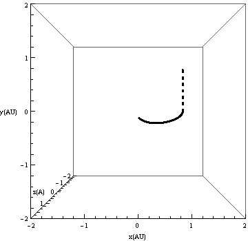
Figure 1: x-y view: The dashed line represents the l propagation of the phonon in the $y$ direction for a flat metric. The initial conditions are $x(0)>1$ and the velocity is $v_{y}(0)=1$. The full line represents the phonon bending in the $x<0$ .

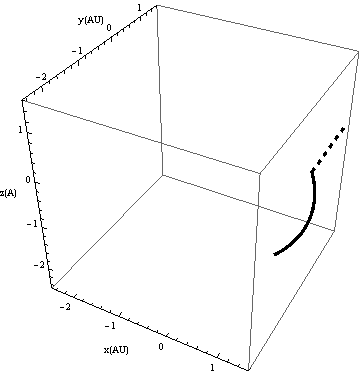
Figure 2: y-z view:The dashed line represents the propagation of the phonon in the $y$ direction for a flat metric. The initial conditions are $x(0)>1$ and the velocity is $v_{y}(0)=1$. The full line represents the phonon bending in the $z<0$ direction .

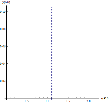
Figure 3: Two dimensional y-x view: Only the propagation for the flat metric in the $y$ direction is seen.

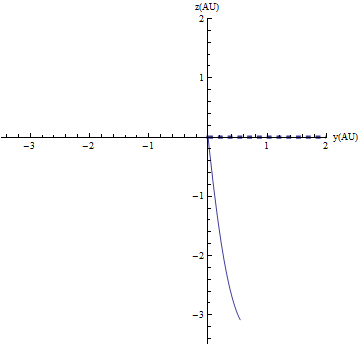
Figure 4: Two dimensional y-z view: The dashed line shows the propagation for a flat metric and the full line shows the phonon bending due to the metric

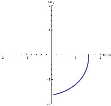
Figure 5: Two dimensional x-z view: The propagation for the flat metric in the $y$ direction is not seen, only the bending of the phonon due to the metric is shown.