Phase diagram and pair Tomonaga-Luttinger liquid
in a Bose-Hubbard model with flat bands

Abstract

To explore superfluidity in flat-band systems, we consider a Bose-Hubbard model on a cross-linked ladder with $\pi$ flux, which has a flat band with a gap between the other band for noninteracting particles, where we study the effect of the on-site repulsion nonperturbatively. For low densities, we find exact degenerate ground states, each of which is a Wigner solid with nonoverlapping Wannier states on the flat band. At higher densities, the many-body system, when projected onto the lower flat band, can be mapped to a spin-chain model. This mapping enables us to reveal the existence of a Tomonaga-Luttinger liquid comprising pairs of bosons. Interestingly, the high- and low- density regions have an overlap, where the two phases coexist.

I Introduction

The macroscopically degenerate manifolds of single-particle states on a flat band provide a unique playground, especially for studying non-perturbative aspects of electron correlations in fermionic lattice models. For example, Lieb, and subsequently Mielke and Tasaki, have shown rigorously that repulsive Hubbard interaction provokes ferri- or ferro-magnetism Lieb89 ; Mielke91 ; Tasaki92 , and localized magnons are discussed in frustrated antiferromagnets Schulenburg02 ; Zhitomirsky04 . In a much wider context, flat-band systems have attracted a renewed attention in terms of topological insulators Hasan10 ; Qi11 , where several constructions were proposed for exactly or nearly flat bands that accommodate nontrivial Chern numbers Katsura10 ; Tang11 ; Sun11 ; Neupert11 . These topological flat bands are reminiscent of Landau levels in the conventional systems in magnetic field and may set the stage for new topological phases when interactions are switched on. Indeed, the Hubbard interaction has been shown to lead to either conventional ferromagnetic states Katsura10 ; Neupert12 or fractional Chern insulators Sheng11 ; Regnault11 , depending on the fermion filling of the flat band.

In the present work, we consider a bosonic system with a Hubbard interaction on a flat-band lattice, which is a cross-linked ladder with $\pi$ flux [Figs. 1(a) and 1(b)]. The basic motivation for going over to a bosonic system is the following. In the fermionic flat-band systems, one important observation is that correlated systems in a flat band are quite distinct from those in the atomic limit (where the hopping in the tight-binding model $\to 0$) Kusakabe94 . Then, an intriguing question arises: Can there be Bose-Einstein condensation (BEC) in flat-band boson systems while we have obviously no BEC in the atomic limit (with an effective mass $\to\infty$)? If we do have states far from those in the atomic limit, we may have a peculiar quantum liquid, or even a possibility of supersolid, i.e., coexistence of condensation with a diagonal long-range order such as charge density wave (CDW). In fact, Huber and Altman have considered this problem, and they concluded that there is a supersolid (superfluid + CDW) region for a chain of triangle and kagome lattices Huber10 .

Our choice of the model [Fig. 1(a)] is inspired by the work of Creutz et al. Creutz99 ; Bermudez09 , which shows that edge states emerge at open boundaries and the fermionic counterpart can be thought of as one-dimensional topological insulators Mazza12 . In this paper, we find that the many-body ground state (GS) exhibits a variety of phases as the density of bosons is varied. While the GS consists of nonoverlapping Wannier states at low densities, we find that Tomonaga-Luttinger liquid (TLL) comprising pairs of bosons (pair TLL) is stabilized at higher densities, where the fundamental degrees of freedom are boson pairs rather than individual bosons. Pair TLL is deduced from the mapping of a boson system onto a spin-1/2 XXZ chain in magnetic field. The validity of the mapping is confirmed by exact diagonalization and the Bethe ansatz solution. The analysis of the spin chain also reveals the coexistence of Wigner solid and pair TLL phases at intermediate densities.

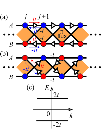
Figure 1: (a) Bose-Hubbard model on a cross-linked ladder with $\pi$ flux. Circles represent sites. $A$ (blue), $B$ (red), and $\ldots,j-1,j,j+1,\ldots$ are chain and rung indices, respectively. While interchain diagonal hopping is $-t$, intrachain hopping is $it$ ($-it$) for along (against) the direction of the arrow, respectively. (b) The same model with interchange of A and B sites on rungs with $j={\rm even}$. (c) Dispersion relation of the present model for the noninteracting case. It has two flat bands at $E=\pm 2t$.

II Formulation

We consider a cross-linked ladder [see Fig. 1(a)] with a Hamiltonian,

$${\cal H} ={\cal H}^{\rm kin}+\frac{U}{2}\sum_{j=1}^{L}\sum_{X=A,B}b_{j}^{X\dagger}b_{j}^{X\dagger}b_{j}^{X}b_{j}^{X},$$

$${\cal H}^{\rm kin} =-t\sum_{j=1}^{L}(e^{i\theta}b_{j}^{A\dagger}b_{j+1}^{A}+e^{-i\theta}b_{j}^{B\dagger}b_{j+1}^{B}$$

$$\qquad\qquad+b_{j}^{A\dagger}b_{j+1}^{B}+b_{j}^{B\dagger}b_{j+1}^{A}+{\rm H.c.}),$$ (1)

with an appropriate local gauge, where $b_{j}^{X\dagger}$ creates a boson, $j$ and $X$ ($=A$, $B$) represent indices for rungs and legs of the ladder, respectively, and $L$ is the length of the ladder (that is, the number of rungs), so the total number of sites is $2L$. The boundary condition is periodic. It is the same as the Creutz model Creutz99 except that particles are not fermions but bosons. Here we focus on the case of $\theta=\pi/2$, which means $\pi$ flux is introduced. Figure 1(b) is the same model with interchanging A and B sites on rungs with $j={\rm even}$. It is useful for analyzing (1) to take the Wannier basis

$$w_{j}^{\pm}=\frac{1}{2}[ib_{j}^{A}-b_{j}^{B}\pm(b_{j+1}^{A}-ib_{j+1}^{B})],$$ (2)

which satisfies bosonic commutation relations: $[w_{j}^{\alpha},w_{j^{\prime}}^{\alpha^{\prime}\dagger}]=\delta_{\alpha,\alpha^{\prime}}\delta_{j,j^{\prime}}$, $[w_{j}^{\alpha},w_{j^{\prime}}^{\alpha^{\prime}}]=[w_{j}^{\alpha\dagger},w_{j^{\prime}}^{\alpha^{\prime}\dagger}]=0$. The kinetic part of the Hamiltonian (1) becomes ${\cal H}^{\rm kin}=\sum_{j=1}^{L}\sum_{\alpha=\pm}\epsilon_{\alpha}w_{j}^{\alpha\dagger}w_{j}^{\alpha}$, where $\epsilon_{\pm}=\pm 2t$. The two energy bands are both flat bands having no wave number dependence (no dispersion), as shown in Fig. 1(c).

III Results

Since the kinetic energy is quenched in the above sense, we have only to consider the particle-particle interaction. The Wannier operator $w_{j}^{\alpha}$ involves $j$ and $j+1$ sites, so that they have only on-site and nearest-neighbor interactions. When the boson density (the averaged number of bosons per site) $\rho\equiv N/(2L)$ is dilute ($\rho\leq 1/4$), we can construct a state that does not feel the interaction by making configurations in which the Wannier state at each site (which we simply call “site” hereafter) is occupied by 0 or 1 particle with no two nearest-neighbor sites occupied [Fig. 2(a)]. Since the kinetic energy is quenched and the interaction term is positive semidefinite, these states are obviously many-body GS of the Hamiltonian ${\cal H}$. This configuration resembles the Wigner solid in an electron gas that minimizes the Coulomb interaction by avoiding overlap, so we call it a Wigner solid hereafter.

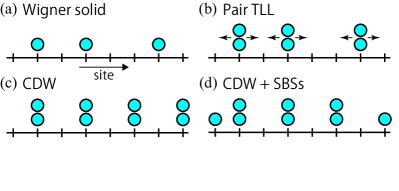
Figure 2: Schematic pictures of (a) Wigner solid, (b) pair TLL, (c) CDW, and (d) CDW with two single-boson sites (SBSs). Particles are localized in panels (a), (c), and (d) while they are mobile (arrows) in panel (b).

For higher density region of $\rho>1/4$, we consider a projection of Hamiltonian onto the lower energy band $\alpha=-$, neglecting the effect of the higher energy band $\alpha=+$ (interband interaction and intraband interaction within the higher band). This approximation is justified when the interaction $U$ is small compared with the hopping $t$. We then obtain

$${\cal H}_{\rm proj}^{\rm int} =\sum_{j=1}^{L}\left[\frac{U}{8}w_{j}^{\dagger}w_{j}^{\dagger}w_{j}w_{j}+\frac{U}{4}w_{j}^{\dagger}w_{j+1}^{\dagger}w_{j}w_{j+1}\right.$$

$$-\frac{U}{16}(w_{j}^{\dagger}w_{j}^{\dagger}w_{j+1}w_{j+1}+\left.{\rm H.c.})\right],$$ (3)

where we have dropped the band index “$-$”. Namely, we end up with on-site repulsion (first term on the right-hand side), nearest-neighbor repulsion (second), and pair hopping of bosons (third), respectively. Remarkably, we have a pair-hopping interaction with a significant magnitude ($U/16$). The sign of this term is irrelevant, since it is altered by a gauge transformation, $w_{j}\to iw_{j}$ (for $j={\rm even}$). We can vary the number of bosons $N$ by adding the chemical potential term $-\mu N\equiv-\mu\sum_{j=1}^{L}w_{j}^{\dagger}w_{j}$ to (3). In the following, we ignore the states in which more than two bosons occupy a single site because the energy would become much higher due to the on-site repulsion. Namely, the number of bosons in a single site is 0, 1, or 2, and these states are denoted by $|0\rangle,|1\rangle,|2\rangle$, respectively. Note that a single boson is immobile because bosons can hop only in pairs, and let us call a site occupied by a single boson a single-boson site (SBS). If we only consider $|0\rangle$ and $|2\rangle$, Eq. (3) can be mapped to a spin-1/2 model by identifying $|0\rangle\mapsto|\downarrow\rangle$ and $|2\rangle\mapsto|\uparrow\rangle$. We introduce spin-1/2 operators $S_{j}^{x(y,z)}$ and $S_{j}^{\pm}=S_{j}^{x}\pm iS_{j}^{y}$, with which we have $w_{j}^{\dagger}w_{j}^{\dagger}w_{j}w_{j}\mapsto 2S_{j}^{z}+1$, $w_{j}^{\dagger}w_{j+1}^{\dagger}w_{j}w_{j+1}\mapsto(2S_{j}^{z}+1)(2S_{j+1}^{z}+1)$, $w_{j}^{\dagger}w_{j}^{\dagger}w_{j+1}w_{j+1}\mapsto 2S_{j}^{+}S_{j+1}^{-}$. The Hamiltonian is then mapped to

$${\cal H}_{S=1/2}= \frac{U}{4}\sum_{j=1}^{L}(-S_{j}^{x}S_{j+1}^{x}-S_{j}^{y}S_{j+1}^{y}+4S_{j}^{z}S_{j+1}^{z})$$

$$\;\;+\frac{5}{4}U\sum_{j=1}^{L}S_{j}^{z}+\frac{3}{8}UL.$$ (4)

This is nothing but the spin-1/2 XXZ model in a magnetic field. The chemical potential term is translated to $-2\mu\sum_{j=1}^{L}(S_{j}^{z}+1/2)$.

If we want to include $|1\rangle$, we only have to map the system to a spin-1 chain ($|0\rangle\mapsto|-1\rangle$, $|1\rangle\mapsto|0\rangle$, $|2\rangle\mapsto|1\rangle$), with which we have $w_{j}^{\dagger}w_{j}^{\dagger}w_{j}w_{j}\mapsto T_{j}^{z}(T_{j}^{z}+1)$, $w_{j}^{\dagger}w_{j+1}^{\dagger}w_{j}w_{j+1}\mapsto(T_{j}^{z}+1)(T_{j+1}^{z}+1)$, $w_{j}^{\dagger}w_{j}^{\dagger}w_{j+1}w_{j+1}\mapsto\frac{1}{2}(T_{j}^{+})^{2}(T_{j+1}^{-})^{2}$, where $T_{j}^{x(y,z)}$ are spin-1 operators and $T_{j}^{\pm}=T_{j}^{x}\pm iT_{j}^{y}$. In this case we have a Hamiltonian

$${\cal H}_{S=1}=\frac{U}{32}\sum_{j=1}^{L}\left[-(T_{j}^{+})^{2}(T_{j+1}^{-})^{2}-(T_{j}^{-})^{2}(T_{j+1}^{+})^{2}\right.$$

$$+\left.8T_{j}^{z}T_{j+1}^{z}\right]+\frac{5}{8}U\sum_{j=1}^{L}T_{j}^{z}+\frac{U}{8}\sum_{j=1}^{L}(T_{j}^{z})^{2}+\frac{1}{4}UL.$$ (5)

These mappings help us investigating GS and low energy excitation structure of (3) below.

Now let us begin with the region of $1/4<\rho<1/2$, where SBSs are adjacent or two bosons occupy the same site. Since the nearest-neighbor repulsion is stronger than on-site repulsion in (3), particles tend to form pairs rather than to occupy adjacent sites. We have performed an exact diagonalization, which demonstrates that the GS of (4) and (5) numerically coincide with each other (see Appendix A). In other words, SBSs are irrelevant, and the use of ${\cal H}_{S=1/2}$ in place of ${\cal H}_{S=1}$ is justified. The $1/4<\rho<1/2$ regime for bosons corresponds to the spin-1/2 XXZ model (4) with nonzero magnetization, where the low-energy excitations are known to be described as TLL induced by external magnetic fields. Since $|\downarrow\rangle$ and $|\uparrow\rangle$ correspond to $|0\rangle$ and $|2\rangle$, respectively, we can translate the state as a “pair TLL” back in the original model. A schematic picture of pair TLL is shown in Fig. 2(b).

We can further make a quantitative analysis since the spin-1/2 XXZ chain is exactly solvable. By solving Bethe ansatz integral equations Qin97 ; Cabra98 , we can determine the spinon velocity $v$ and the Luttinger parameter $K$, which characterize correlation functions as

$$\langle n_{r}n_{0}\rangle\simeq 4\rho^{2}-2K(\pi r)^{-2}+c_{1}\cos(2\pi\rho r)r^{-2K},$$

$$\langle w_{r}^{\dagger}w_{r}^{\dagger}w_{0}w_{0}\rangle\simeq(-)^{r}c_{2}r^{-\frac{1}{2K}}+(-)^{r}c_{3}\cos(2\pi\rho r)r^{-2K-\frac{1}{2K}}.$$

Here the lattice constant is taken to be unity, $n_{r}=w_{r}^{\dagger}w_{r}$, and $c_{1},c_{2},c_{3}$ are nonuniversal constants. In the present case, where $1/4\leq K\leq 1/2$, $\langle w_{r}^{\dagger}w_{r}^{\dagger}w_{0}w_{0}\rangle$ decays faster than $\langle n_{r}n_{0}\rangle$. Note that collective excitations in TLL are gapless in contrast to the gapped excitations for creating SBSs. This fact again justifies the neglect of SBSs in taking the low-energy effective Hamiltonian.

Here we can raise an intriguing question: Can Wigner solid and pair TLL phases coexist? Since each boundary between the two phases costs surface energy, there should be a single boundary, if any. We assume that the proportion of Wigner solid phase is $x\;\;(0\leq x\leq 1)$, i.e., Wigner solid phase has $xL/2$ bosons occupying $2xL$ sites, while pair TLL phase has $N-xL/2$ bosons occupying $2(1-x)L$ sites. This pair TLL translates into the spin-1/2 chain with magnetization $M=1/2-(\rho-x/4)/(1-x)$ (with the saturated magnetization corresponding to 1/2), and the GS energy per site $e_{\rm TLL}(\rho,x)$ can be obtained by solving the Bethe-ansatz equations Qin97 ; Cabra98 . The energy in the total system is $e(\rho,x)\equiv(1-x)e_{\rm TLL}(\rho,x)$, since the Wigner solid phase has zero energy. We can then determine $x$ by minimizing $e(\rho,x)$. Figure  3(a) displays $e(\rho,x)-e_{\rm min}$ ($e_{\rm min}$: the minimum value) against $x$. We find that for $\rho\leq 0.25$ the minimum occurs at $x=1$ (a pure Wigner solid phase), while for $\rho\geq 0.35$ the minimum locates at $x=0$ (a pure pair TLL phase). In the intermediate regions ($0.25\leq\rho\leq 0.35$) we do have a coexistence of the two phases (with $0<x<1$).

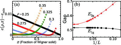
Figure 3: (a) The GS energy per site above its minimum, $e(\rho,x)-e_{\rm min}$, against the fraction of Wigner solid phase $x$ in the density region $0.25\leq\rho\leq 0.35$. (b) System-size ($L$) dependence of the energy of the state with two adjacent SBSs ($E_{1{\rm g}}$) and that of the first excited state without SBSs ($E_{2{\rm g}}$) at $\rho=1/2$. Solid curves represent the extrapolation by fourth-order polynomials, while arrows are the analytically obtained values. The energy unit is $U=1$.

Finally, we consider the $\rho=1/2$ case. Since the GSs of (4) and (5) coincide according to numerical diagonalization, the spin-1/2 description is still valid. However, we have to be careful about the excited states involving SBSs because the $\rho=1/2$ case corresponds to the XXZ chain without magnetization and has an excitation gap. The lowest two levels are doubly degenerate GSs, which have a Néel order due to a strong Ising anisotropy in the XXZ description (4). This state translates to a charge density wave (CDW) of pair bosons [Fig. 2(c)]. Let us consider the configuration that contains two adjacent SBSs [Fig. 2(d)]. It translates into a system of length $L-2$ having $N-2$ bosons with open boundary condition, for which the Hamiltonian is Eq. (4) with the summation changed to $\sum_{j=2}^{L-1}$ (with $j=1$ and $L$ occupied by SBSs) and a constant ($U/4$) subtracted. We have confirmed that the two lowest energy levels of this open chain agree with the lowest two excitations. These levels correspond to CDW of $N-2$ bosons (Néel state in the spin model) in a chain of length $L-2$.

Upon a closer look, the energy of the state with two adjacent SBSs ($E_{1{\rm g}}$) and that of the first excited state without SBSs ($E_{2{\rm g}}$) are calculated by exact diagonalization for various system sizes, which is shown in Fig. 3(b). The thermodynamic limit of $E_{1{\rm g}}$ and $E_{2{\rm g}}$ is determined exactly with the Bethe ansatz Batchelor90 ; Kapustin96 as $E_{1{\rm g}}^{(L\to\infty)}\simeq 0.515877$ and $E_{2{\rm g}}^{(L\to\infty)}\simeq 0.539548$ (see Appendix C). Here, we take the energy unit as $U=1$. If we extrapolate $E_{1{\rm g}}$ and $E_{2{\rm g}}$ with fourth-order polynomials [solid curves in Fig. 3(b)], the thermodynamic limit agrees with the Bethe ansatz result accurately. Thus, it is confirmed that the low-energy structure, except for the midgap state (corresponding to $E_{1{\rm g}}$), is described well by the effective spin-1/2 model (4).

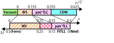
Figure 4: GS phase diagram as a function of the chemical potential $\mu$ or the density $\rho$. WS and FITLL stand for Wigner solid and field-induced TLL, respectively. The bottom axis is the corresponding phase diagram for the spin-1/2 XXZ chain as a function of magnetization $M$.

Now we can summarize the phase diagram in Fig. 4. The transition from Wigner solid to the pair TLL is of the first order, accompanied by a region with coexistence of the two phases. The transition from pair TLL to CDW translates to that from field-induced TLL phase to Néel state in spin-1/2 XXZ model, which belongs to Dzhaparidze-Nersesyan-Pokrovsky-Talapov universality class Cabra98 . The relation between chemical potential $\mu$ and boson density $\rho$ in the pair TLL phase corresponds to the $M$-$H$ curve (magnetization vs magnetic field) in the XXZ model.

IV Summary and discussion

We have studied how the repulsive interaction exerts an effect on bosons in a flat-band Bose-Hubbard model on a cross-linked ladder with $\pi$ flux. In the low boson-density region $\rho\leq 1/4$, the GS is Wigner solid with nonoverlapping Wannier states. We have revealed an existence of pair TLL when $\mu$ is increased, after the first-order transition accompanying a phase coexistence region. Finally, the GS becomes CDW at $\rho=1/2$. The phase diagram and low-energy excitation structure are analyzed through the mapping to an effective spin-1/2 XXZ chain, which is confirmed by exact diagonalization and the Bethe ansatz.

Our model is relevant to a Bose-Hubbard model on a diamond chain, which has been realized experimentally Gladchenko09 . A pair TLL is also pointed out in this diamond chain with $\pi$ flux Vidal00 ; Doucot02 as a “nematic Luttinger liquid,” but they employed the mapping to the classical rotator model. Their model has three flat bands Gulacsi07 at $E=0,\pm 2t$, and its analysis can be done in the same way as we do here. If the Hamiltonian is projected onto the lowest band with $E=-2t$, the on-site repulsion is stronger than the nearest-neighbor one. Thus the system is always in the Wigner solid phase while the pair TLL does not appear. The projection to the $E=0$ band would provide a model similar to the effective model for the cross-linked ladder, but such a projection would not be justified, since the effect of $E=\pm 2t$ bands is not negligible in both low- and high-boson-density regions. We can prove that the lower band in our model corresponds to $E=0$ band in the diamond chain by integrating out the vertex having four edges of the latter model. Therefore, we believe that our approach is more rigorous in demonstrating the existence of the pair TLL phase.

Recent progress in cold atom physics has enabled experimentalists to realize bosons with “synthetic gauge fields” Lin09 , and our result is expected to be tested with bosons trapped in an optical lattice with a ladder configuration. While we have concentrated here on a bosonic system, searching for nontrivial phases in fermionic flat-band systems Filho08 ; Lopes11 is an interesting future problem. If two chains are considered as spin up and spin down, Hamiltonian (1) may be regarded as a one-dimensional electron system with a spin-orbit coupling. Also, solving a problem by mapping to spin chains reminds us of the Tao-Thouless (thin torus) limit Tao83 ; Nakamura10 of the fractional quantum Hall system. Considering higher-dimensional flat-band systems is another direction to study Huber10 .

Appendix A Justifications of the mapping
to the spin-1/2 chain

In order to study the Hamiltonian (3), we have exploited the mapping to a spin chain model. When SBSs are neglected, the mapped model is a spin-1/2 chain with a Hamiltonian (4) while if we include SBSs we have an $S=1$ model (5)

Table 1: The GS energies for the spin models (4) and (5), respectively, of length $L=16$ calculated with exact diagonalization. The GS energy is shown in the unit of $U=1$.

$N$	$\rho$	GS energy of (4)	GS energy of (5)
8	0.2500	0.1453388529	0.0000000000
10	0.3125	0.3214844344	0.3214844344
12	0.3750	0.6206828185	0.6206828185
14	0.4375	1.0891052450	1.0891052450
16	0.5000	1.7536447794	1.7536447794

To justify the neglect of SBSs, we have performed an exact diagonalization. The GS energies of (4) and (5) of length $L=16$ are respectively shown in Table 1. For the number of bosons $N>L/2$ ($\rho>1/4$), Hamiltonians (4) and (5) are seen to indeed share the same GSs. For $0\leq N\leq L/2$ ($0\leq\rho\leq 1/4$), on the other hand, the GS of (5) is the zero-energy state (Wigner solid), which is not the GS of (4). In Table 1, $N=10$ $(\rho=5/16)$ should correspond to the coexistence region, but the energy of the coexistence state is raised due to the surface energy in finite systems, and the pair Tomonaga-Luttinger liquid (pair TLL) becomes the GS.

Appendix B Low-energy excitation structure
at $\rho=1/2$

Table 2: Several lowest energy levels of $S=1$ model (5) with $L=16$ calculated with exact diagonalization. The GS energy is shown in the unit of $U=1$.

	Energy	Degeneracy	Number of SBSs
1	1.7536447794	1	0
2	1.7541665514	1	0
3	2.2686557182	16	2
4	2.2709315403	16	2
5	2.3541625572	1	0
6	2.3668727422	1	0
7	2.4029012587	2	0
8	2.4115680946	2	0

For the case of $\rho=1/2$, the spin-1/2 description is still valid, since the GSs of (4) and (5) coincide with each other for $N=16$ as seen in Table 1. However, we have to pay attention to the excited states involving SBSs because the $\rho=1/2$ case corresponds to the XXZ chain without magnetization for which an excitation gap exists. Several lower-most levels of the spin-1 model (5) are displayed in Table 2. The lowest two levels are doubly-degenerate GSs (although the degeneracy is slightly lifted due to a finite-size effect), which have a Néel order due to the strong Ising anisotropy in the XXZ description (4). This state translates to a charge density wave (CDW) of pair bosons.

The first two excited levels in Table 2 do not appear in the energy levels of (4), and hence they should correspond to the configuration involving SBSs. The system having two adjacent SBSs at site $j=1$ and $L$ can be mapped to a spin-1/2 chain with open boundary conditions such as

$${\cal H}_{S=1/2}^{\rm open}= \frac{U}{4}\sum_{j=2}^{L-2}(-S_{j}^{x}S_{j+1}^{x}-S_{j}^{y}S_{j+1}^{y}+4S_{j}^{z}S_{j+1}^{z})$$

$$+\frac{5}{4}U\sum_{j=2}^{L-1}S_{j}^{z}+\frac{3}{8}UL-\frac{U}{4}.$$ (6)

We have confirmed that the two lowest energy levels of (6) do agree with the first two excited states in Table 2. These levels correspond to CDW of $N-2$ bosons (Néel state in the spin model) in a chain of length $L-2$ with open boundary condition. Each of them is $L$-fold degenerated, since the neighboring SBSs have a translational invariance.

Appendix C Exact results from Bethe ansatz

As for the energy of the state with two adjacent SBSs ($E_{1{\rm g}}$) and that of the first excited state without SBSs ($E_{2{\rm g}}$), we can notice that the thermodynamic limit can be calculated exactly with the Bethe ansatz Batchelor90 ; Kapustin96 . Let us define $\theta\equiv\cosh^{-1}\Delta>0$, where $\Delta$ represents the Ising anisotropy of the XXZ chain. In the present case $\Delta=4$, hence $\theta=\ln(4+\sqrt{17})$, and we have

$$E_{1{\rm g}}^{(L\to\infty)} =-2e_{0}+E_{\rm surf}-1/4\simeq 0.515877,$$

$$E_{2{\rm g}}^{(L\to\infty)} =\frac{\sinh\theta}{4}\prod_{n=1}^{\infty}\left(\frac{{\rm e}^{n\theta}-1}{{\rm e}^{n\theta}+1}\right)^{2}\simeq 0.539548,$$

where

$$e_{0}= \frac{1}{16}\cosh\theta-\frac{1}{8}\sinh\theta\left(1+4\sum_{n=1}^{\infty}\frac{1}{{\rm e}^{2n\theta}+1}\right),$$

$$E_{\rm surf}= -\frac{\Delta}{16}+\frac{1}{2}\sinh\theta\left[\frac{1}{4}+\sum_{n=1}^{\infty}\frac{{\rm e}^{2n\theta}-1}{{\rm e}^{4n\theta}+1}+\sum_{n=1}^{\infty}\frac{(-1)^{n}}{{\rm e}^{2n\theta}+1}\right],$$

represent the ground-state energy per site Batchelor90 and the surface energy Kapustin96 of the XXZ chain, respectively. Here, the energy unit $U=1$ is taken.

References

- (1) E. H. Lieb, Phys. Rev. Lett. 62, 1201 (1989).
- (2) A. Mielke, J. Phys. A: Math. Gen. 24, L73 (1991); ibid 24, 3311 (1991).
- (3) H. Tasaki, Phys. Rev. Lett. 69, 1608 (1992).
- (4) J. Schulenburg, A. Honecker, J. Schnack, J. Richter, and H.-J. Schmidt, Phys. Rev. Lett. 88, 167207 (2002).
- (5) M. E. Zhitomirsky, H. Tsunetsugu, Phys. Rev. B 70, 100403(R) (2004).
- (6) M. Z. Hasan and C. L. Kane, Rev. Mod. Phys. 82, 3045 (2010).
- (7) X.-L. Qi and S.-C. Zhang, Rev. Mod. Phys. 83, 1057 (2011).
- (8) H. Katsura, I. Maruyama, A. Tanaka, and H. Tasaki, Europhys. Lett. 91, 57007 (2010).
- (9) E. Tang, J.-W. Mei, and X.-G. Wen, Phys. Rev. Lett. 106, 236802 (2011).
- (10) K. Sun, Z. Gu, H. Katsura, and S. Das Sarma, Phys. Rev. Lett. 106, 236803 (2011).
- (11) T. Neupert, L. Santos, C. Chamon, and C. Mudry, Phys. Rev. Lett. 106, 236804 (2011).
- (12) T. Neupert, L. Santos, S. Ryu, C. Chamon, and C. Mudry, Phys. Rev. Lett. 108, 046806 (2012).
- (13) D. N. Sheng, Z.-C. Gu, K. Sun, and L. Sheng, Nat. Commun. 2, 389 (2011).
- (14) N. Regnault and B. A. Bernevig, Phys. Rev. X 1, 021014 (2011).
- (15) K. Kusakabe and H. Aoki, Phys. Rev. Lett. 72, 144 (1994).
- (16) S. D. Huber and E. Altman, Phys. Rev. B 82, 184502 (2010).
- (17) M. Creutz, Phys. Rev. Lett. 83, 2636 (1999).
- (18) A. Bermudez, D. Patanè, L. Amico, and M. A. Martin-Delgado, Phys. Rev. Lett. 102, 135702 (2009).
- (19) L. Mazza, A. Bermudez, N. Goldman, M. Rizzi, M. A. Martin-Delgado, and M. Lewenstein, New J. Phys. 14, 015007 (2012).
- (20) S. Qin, M. Fabrizio, L. Yu, M. Oshikawa, and I. Affleck, Phys. Rev. B 56, 9766 (1997).
- (21) D. C. Cabra, A. Honecker, and P. Pujol, Phys. Rev. B 58, 6241 (1998).
- (22) M. T. Batchelor and C. J. Hamer, J. Phys. A: Math. Gen. 23, 761 (1990).
- (23) A. Kapustin and S. Skorik, J. Phys. A: Math. Gen. 29, 1629 (1996).
- (24) S. Gladchenko, D. Olaya, E. Dupont-Ferrier, B. Douçot, L. B. Ioffe, and M. E. Gershenson, Nat. Phys. 5, 48 (2009).
- (25) J. Vidal, B. Douçot, R. Mosseri, and P. Butaud, Phys. Rev. Lett. 85, 3906 (2000).
- (26) B. Douçot and J. Vidal, Phys. Rev. Lett. 88, 227005 (2002).
- (27) Z. Gulácsi, A. Kampf, and D. Vollhardt, Phys. Rev. Lett. 99, 026404 (2007).
- (28) Y.-J. Lin, R. L. Compton, K. Jiménez-García, J. V. Porto, and I. B. Spielman, Nature (London) 462, 628 (2009).
- (29) R. R. Montenegro-Filho and M. D. Coutinho-Filho, Phys. Rev. B 74, 125117 (2006).
- (30) A. A. Lopes and R. G. Dias, Phys. Rev. B 84, 085124 (2011).
- (31) R. Tao and D. J. Thouless, Phys. Rev. B 28, 1142 (1983).
- (32) M. Nakamura, E. J. Bergholtz, and J. Suorsa, Phys. Rev. B 81, 165102 (2010).