Generating Explanations for Biomedical Queries

Abstract

We introduce novel mathematical models and algorithms to generate (shortest or $k$ different) explanations for biomedical queries, using answer set programming. We implement these algorithms and integrate them in BioQuery-ASP. We illustrate the usefulness of these methods with some complex biomedical queries related to drug discovery, over the biomedical knowledge resources PharmGKB, DrugBank, BioGRID, CTD, SIDER, Disease Ontology and Orphadata.

1 Introduction

Recent advances in health and life sciences have led to generation of a large amount of biomedical data, represented in various biomedical databases or ontologies. That these databases and ontologies are represented in different formats and constructed/maintained independently from each other at different locations, have brought about many challenges for answering complex biomedical queries that require integration of knowledge represented in these ontologies and databases. One of the challenges for the users is to be able to represent such a biomedical query in a natural language, and get its answers in an understandable form. Another challenge is to extract relevant knowledge from different knowledge resources, and integrate them appropriately using also definitions, such as, chains of gene-gene interactions, cliques of genes based on gene-gene relations, or similarity/diversity of genes/drugs. Furthermore, once an answer is found for a complex query, the experts may need further explanations about the answer.

Table 1 displays a list of complex biomedical queries that are important from the point of view of drug discovery. In the queries, drug-drug interactions present negative interactions among drugs, and gene-gene interactions present both negative and positive interactions among genes. Consider, for instance the query Q6. New molecule synthesis by changing substitutes of parent compound may lead to different biochemical and physiological effects; and each trial may lead to different indications. Such studies are important for fast inventions of new molecules. For example, while developing the drug Lovastatin (a member of the drug class of Hmg-coa reductase inhibitors, used for lowering cholesterol) from Aspergillus terreus (a sort of fungus) in 1979, scientists at Merck derived a new molecule named Simvastatin that also belongs to the same drug category (a hypolipidemic drug used to control elevated cholesterol) targeting the same gene. Therefore, identifying genes targeted by a group of drugs automatically by means of queries like Q6 may be useful for experts.

Once an answer to a query is found, the experts may ask for an explanation to have a better understanding. For instance, an answer for the query Q3 in Table 1 is “ADRB1”. A shortest explanation for this answer is as follows:

• The drug Epinephrine targets the gene ADRB1 according to CTD.
  The gene DLG4 interacts with the gene ADRB1 according to BioGRID.

An answer for the query Q8 is “CASK”. A shortest explanation for this answer is as follows:

The distance of the gene CASK from the start gene is 2.

The gene CASK interacts with the gene DLG4 according to BioGRID.

The distance of the gene DLG4 from the start gene is 1.

The gene DLG4 interacts with the gene ADRB1 according to BioGRID.

ADRB1 is the start gene.

(Statements with more indentations provide explanations for statements with less indentations.)

Table 1: A list of complex biomedical queries.

Q1 What are the drugs that treat the disease Asthma and that target the gene ADRB1? Q2 What are the side effects of the drugs that treat the disease Asthma and that target the gene ADRB1? Q3 What are the genes that are targeted by the drug Epinephrine and that interact with the gene DLG4? Q4 What are the genes that interact with at least $3$ genes and that are targeted by the drug Epinephrine? Q5 What are the drugs that treat the disease Asthma or that react with the drug Epinephrine? Q6 What are the genes that are targeted by all the drugs that belong to the category Hmg-coa reductase inhibitors? Q7 What are the cliques of $5$ genes, that contain the gene DLG4? Q8 What are the genes that are related to the gene ADRB1 via a gene-gene interaction chain of length at most $3$? Q9 What are the $3$ most similar genes that are targeted by the drug Epinephrine? Q10 What are the genes that are related to the gene DLG4 via a gene-gene interaction chain of length at most $3$ and that are targeted by the drugs that belong to the category Hmg-coa reductase inhibitors? Q11 What are the drugs that treat the disease Depression and that do not target the gene ACYP1? Q12 What are the symptoms of diseases that are treated by the drug Triadimefon? Q13 What are the $3$ most similar drugs that target the gene DLG4? Q14 What are the $3$ closest drugs to the drug Epinephrine?

To address the first two challenges described above (i.e., representing complex queries in natural language and finding answers to queries efficiently), novel methods and a software system, called BioQuery-ASP [Erdem et al. (2011)] (Figure 1), have been developed using Answer Set Programming (ASP) [Marek and Truszczyński (1999), Niemelä (1999), Lifschitz (2002), Baral (2003), Lifschitz (2008), Brewka et al. (2011)]:

• Erdem and Yeniterzi [Erdem and Yeniterzi (2009)] developed a controlled natural language, BioQuery-CNL, for expressing biomedical queries related to drug discovery. For instance, queries Q1–Q10 in Table 1 are in this language. Recently, this language has been extended (called BioQuery-CNL*) to cover queries Q11–Q13 [Oztok (2012)]. Some algorithms have been introduced to translate a given query in BioQuery-CNL (resp. BioQuery-CNL*) to a program in ASP as well.

• Bodenreider et al. [Bodenreider et al. (2008)] introduced methods to extract biomedical information from various knowledge resources and integrate them by a rule layer. This rule layer not only integrates those knowledge resources but also provides definitions of auxiliary concepts.

• Erdem et al. [Erdem et al. (2011)] have introduced an algorithm for query answering by identifying the relevant parts of the rule layer and the knowledge resources with respect to a given query.

The details of representing biomedical queries in natural language and answering them using ASP are explained in a companion article. The focus of this article is the last challenge: generating explanations for biomedical queries.

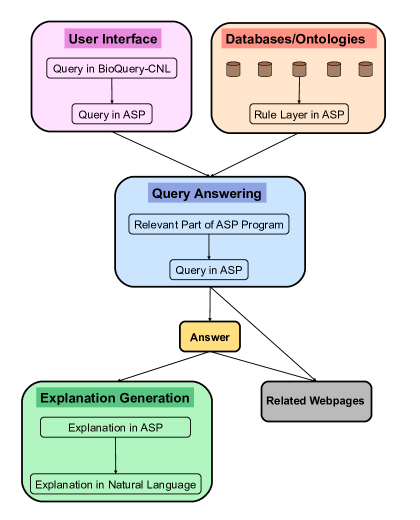
Figure 1: System overview of BioQuery-ASP.

Most of the existing biomedical querying systems (e.g., web services built over the available knowledge resources) support keyword search but not complex queries like the queries in Table 1. None of the existing systems can provide informative explanations about the answers, but point to related web pages of the knowledge resources available online.

The contributions of this article can be summarized as follows.

• We have formally defined “explanations” in ASP, utilizing properties of programs and graphs. We have also defined variations of explanations, such as “shortest explanations” and “$k$ different explanations”.

• We have introduced novel generic algorithms to generate explanations for biomedical queries. These algorithms can compute shortest or $k$ different explanations. We have analyzed the termination, soundness, and complexity of those algorithms.

• We have developed a computational tool, called ExpGen-ASP, that implements these explanation generation algorithms.

• We have showed the applicability of our methods to generate explanations for answers of complex biomedical queries related to drug discovery.

• We have embedded ExpGen-ASP into BioQuery-ASP so that the experts can obtain explanations regarding the answers of biomedical queries, in a natural language.

The rest of the article is organized as follows. In Section 2, we provide a summary of Answer Set Programming. Next, in Section 3, we give an overview of BioQuery-ASP, in particular, the earlier work done on answering biomedical queries in ASP. Then, in Sections 4–6, we provide some definitions and algorithms related to generating shortest or $k$ different explanations for an answer, also in ASP. Next, Section 7 illustrates the usefulness of these algorithms on some complex queries over the biomedical knowledge resources PharmGKB [McDonagh et al. (2011)], DrugBank [Knox et al. (2010)], BioGRID [Stark et al. (2006)], CTD [Davis et al. (2011)], SIDER [Kuhn et al. (2010)], Disease Ontology [Schriml et al. (2012)] and Orphadata. In Sections 8 and 9, we discuss how to present explanations to the user in a natural language, and embedding of these algorithms in BioQuery-ASP. In Section 10, we provide a detailed analysis of the related work on “justifications” [Pontelli et al. (2009)] in comparison to explanations; and in Section 11, we briefly discuss other related work. We conclude in Section 12 by summarizing our contributions and pointing out some possible future work. Proofs are provided in the online appendix of the paper.

2 Answer Set Programming

Answer Set Programming (ASP) [Marek and Truszczyński (1999), Niemelä (1999), Lifschitz (2002), Baral (2003), Lifschitz (2008), Brewka et al. (2011)] is a form of declarative programming paradigm oriented towards solving combinatorial search problems as well as knowledge-intensive problems. The idea is to represent a problem as a “program” whose models (called “answer sets” [Gelfond and Lifschitz (1988), Gelfond and Lifschitz (1991)]) correspond to the solutions. The answer sets for the given program can then be computed by special implemented systems called answer set solvers. ASP has a high-level representation language that allows recursive definitions, aggregates, weight constraints, optimization statements, and default negation.

ASP also provides efficient solvers, such as clasp [Gebser et al. (2007)]. Due to the continuous improvement of the ASP solvers and highly expressive representation language of ASP which is supported by a strong theoretical background that results from a years of intensive research, ASP has been applied fruitfully to a wide range of areas. Here are, for instance, three applications of ASP used in industry:

• Decision Support Systems: An ASP-based system was developed to help flight controllers of space shuttle solve some planning and diagnostic tasks [Nogueira et al. (2001)] (used by United Space Alliance).

• Automated Product Configuration: A web-based commercial system uses an ASP-based product configuration technology [Tiihonen et al. (2003)] (used by Variantum Oy).

• Workforce Management: An ASP-based system is developed to build teams of employees to handle incoming ships by taking into account a variety of requirements, e.g., skills, fairness, regulations [Ricca et al. (2012)] (used by Gioia Tauro seaport).

Let us briefly explain the syntax and semantics of ASP programs and describe how a computational problem can be solved in ASP.

2.1 Programs

Syntax

The input language of ASP programs are composed of three sets namely constant symbols, predicate symbols, and variable symbols where intersection of constant symbols and variable symbols is empty. The basic elements of the ASP programs are atoms. An atom $p(\vec{t})$ is composed of a predicate symbol $p$ and terms $\vec{t}=t_{1},\dots,t_{k}$ where each $t_{i}$ ($1\leq i\leq k$) is either a constant or a variable. A literal is either an atom $p(\vec{t})$ or its negated form $not\ p(\vec{t})$.

An ASP program is a finite set of rules of the form:

$$A\leftarrow A_{1},\ldots,A_{k},not\ A_{k+1},\ldots,not\ A_{m}$$ (1)

where $m\geq k\geq 0$ and each $A_{i}$ is an atom; whereas, $A$ is an atom or $\bot$.

For a rule $r$ of the form (1), $A$ is called the head of the rule and denoted by $H(r)$. The conjunction of the literals $A_{1},\ldots,A_{k},not\ A_{k+1},\ldots,not\ A_{m}$ is called the body of $r$. The set $\{A_{1},...,A_{k}\}$ of atoms (called the positive part of the body) is denoted by $B^{+}(r)$, and the set $\{A_{k+1},...,A_{m}\}$ of atoms (called the negative part of the body) is denoted by $B^{-}(r)$, and all the atoms in the body are denoted by $B(r)=B^{+}(r)\cup B^{-}(r)$.

We say that a rule $r$ is a fact if $B(r)=\emptyset$, and we usually omit the $\leftarrow$ sign. Furthermore, we say that a rule $r$ is a constraint if the head of $r$ is $\bot$, and we usually omit the $\bot$ sign.

Semantics (Answer Sets)

Answer sets of a program are defined over ground programs. We call an atom, rule, or program ground, if it does not contain any variables. Given a program $\Pi$, the set ${\mathcal{}U}_{\Pi}$ represents all the constants in $\Pi$, and the set ${\mathcal{}B}_{\Pi}$ represents all the ground atoms that can be constructed from atoms in $\Pi$ with constants in ${\mathcal{}U}_{\Pi}$. Also, $Ground(\Pi)$ denotes the set of all the ground rules which are obtained by substituting all variables in rules with the set of all possible constants in ${\mathcal{}U}_{\Pi}$.

A subset $I$ of ${\mathcal{}B}_{\Pi}$ is called an interpretation for $\Pi$. A ground atom $p$ is true with respect to an interpretation $I$ if $p\in I$; otherwise, it is false. Similarly, a set $S$ of atoms is true (resp., false) with respect to $I$ if each atom $p\in S$ is true (resp., false) with respect to $I$. An interpretation $I$ satisfies a ground rule $r$, if $H(r)$ is true with respect to $I$ whenever $B^{+}(r)$ is true and $B^{-}(r)$ is false with respect to $I$. An interpretation $I$ is called a model of a program $\Pi$ if it satisfies all the rules in $\Pi$.

The reduct $\Pi^{I}$ of a program $\Pi$ with respect to an interpretation $I$ is defined as follows:

$$\Pi^{I}=\{H(r)\leftarrow B^{+}(r)\ |\ r\in Ground(\Pi)\ s.t.\ I\cap B^{-}(r)=\emptyset\}$$

An interpretation $I$ is an answer set for a program $\Pi$, if it is a subset-minimal model for $\Pi^{I}$, and $AS(\Pi)$ denotes the set of all the answer sets of a program $\Pi$.

For example, consider the following program $\Pi_{1}$:

$$p\leftarrow not\ q$$ (2)

and take an interpretation $I=\{p\}$. The reduct $\Pi_{1}^{I}$ is as follows:

$$p$$ (3)

The interpretation $I$ is a model of the reduct (3). Let us take a strict subset $I^{\prime}$ of $I$ which is $\emptyset$. Then, the reduct $\Pi_{1}^{I^{\prime}}$ is again equal to (3); however, $I^{\prime}$ does not satisfy (3). Therefore, $I=\{p\}$ is a subset-minimal model; hence an answer set of $\Pi_{1}$. Note also that $\{p\}$ is the only answer set of $\Pi$.

2.2 Generate-And-Test Representation Methodology with Special ASP Constructs

The idea of ASP [Lifschitz (2008)] is to represent a computational problem as a program whose answer sets correspond to the solutions of the problem, and to find the answer sets for that program using an answer set solver.

When we represent a problem in ASP, two kinds of rules play an important role: those that “generate” many answer sets corresponding to “possible solutions”, and those that can be used to “eliminate” the answer sets that do not correspond to solutions. The rules

$$\begin{array}[]{l}p\leftarrow not\ q\\ q\leftarrow not\ p\end{array}$$ (4)

are of the former kind: they generate the answer sets $\{p\}$ and $\{q\}$. Constraints are of the latter kind. For instance, adding the constraint

$$\leftarrow p$$

to program (4) eliminates the answer sets for the program that contain $p$.

In ASP, we use special constructs of the form

$$\{A_{1},\dots,A_{n}\}^{c}$$ (5)

(called choice expressions), and of the form

$$l\leq\{A_{1},\dots,A_{m}\}\leq u$$ (6)

(called cardinality expressions) where each $A_{i}$ is an atom and $l$ and $u$ are nonnegative integers denoting the “lower bound” and the “upper bound” [Simons et al. (2002)]. Programs using these constructs can be viewed as abbreviations for normal nested programs defined in [Ferraris and Lifschitz (2005)]. Expression (5) describes subsets of $\{A_{1},\dots,A_{n}\}$. Such expressions can be used in heads of rules to generate many answer sets. For instance, the answer sets for the program

$$\{p,q,r\}^{c}\ \leftarrow\$$ (7)

are arbitrary subsets of $\{p,q,r\}$. Expression (6) describes the subsets of the set $\{A_{1},\dots,A_{m}\}$ whose cardinalities are at least $l$ and at most $u$. Such expressions can be used in constraints to eliminate some answer sets. For instance, adding the constraint

$$\leftarrow\ 2\leq\{p,q,r\}$$

to program (7) eliminates the answer sets for (7) whose cardinalities are at least 2. We abbreviate the rules

$$\begin{array}[]{l}\{A_{1},\dots,A_{m}\}^{c}\leftarrow\hbox{Body\/}\\ \leftarrow not\ (l\leq\{A_{1},\dots,A_{m}\})\\ \leftarrow not\ (\{A_{1},\dots,A_{m}\}\leq u)\end{array}$$

by the rule

$$l\leq\{A_{1},\dots,A_{m}\}^{c}\leq u\leftarrow\hbox{Body\/}.$$

In ASP, there are also special constructs that are useful for optimization problems. For instance, to compute answer sets that contain the maximum number of elements from the set $\{A_{1},\ldots,A_{m}\}$, we can use the following optimization statement.

$${maximize}\langle\{A_{1},\ldots,A_{m}\}\rangle$$

2.3 Presenting Programs to Answer Set Solvers

Once we represent a computational problem as a program whose answer sets correspond to the solutions of the problem, we can use an answer set solver to compute the solutions of the problem. To present a program to an answer set solver, like clasp, we need to make some syntactic modifications.

Recall that answer sets for a program are defined over ground programs. Thus, the input of ASP solvers should be ground instantiations of the programs. For that, programs go through a “grounding” phase in which variables in the program (if exists) are substituted by constants. For clasp, we use the “grounder” gringo [Gebser et al. (2011)].

Although the syntax of the input language of gringo is somewhat more restricted than the class of programs defined above, it provides a number of useful special constructs. For instance, the head of a rule can be an expression of one of the forms

$$\begin{array}[]{l}\{A_{1},\dots,A_{n}\}^{c}\\ l\leq\{A_{1},\dots,A_{n}\}^{c}\\ \{A_{1},\dots,A_{n}\}^{c}\leq u\\ l\leq\{A_{1},\dots,A_{n}\}^{c}\leq u\end{array}$$

but the superscript ^c and the sign $\leq$ are dropped. The body can also contain cardinality expressions but the sign $\leq$ is dropped. In the input language of gringo, :- stands for $\leftarrow$, and each rule is followed by a period. For facts $\leftarrow$ is dropped. For instance, the rule

$$1\leq\{p,q,r\}^{c}\leq 1\leftarrow$$

can be presented to gringo as follow:

1{p,q,r}1.

Variables in a program are represented by strings whose initial letters are capitalized. The constants and predicate symbols, on the other hand, start with a lowercase letter. For instance, the program $\Pi_{n}$

$$p_{i}\leftarrow\hbox{not\/}\ \ p_{i+1}\qquad(1\leq i\leq n)$$

can be presented to gringo as follows:

index(1..n).
p(I) :- not p(I+1), index(I).

Here, the auxiliary predicate index is a “domain predicate” used to describe the ranges of variables. Variables can be also used “locally” to describe the list of formulas. For instance, the rule

$$1\leq\{p_{1},\dots,p_{n}\}\leq 1$$

can be expressed in gringo as follows

index(1..n).
1{p(I) : index(I)}1.

3 Answering Biomedical Queries

We have earlier developed the software system BioQuery-ASP [Erdem et al. (2011)] (see Figure 1) to answer complex queries that require appropriate integration of relevant knowledge from different knowledge resources and auxiliary definitions such as chains of drug-drug interactions, cliques of genes based on gene-gene relations, or similar/diverse genes. As depicted in Figure 1, BioQuery-ASP takes a query in a controlled natural language and transforms it into ASP. Meanwhile, it extracts knowledge from biomedical databases and ontologies, and integrates them in ASP. Afterwards, it computes an answer to the given query using an ASP solver.

Let us give an example to illustrate these stages; the details of representing biomedical queries in natural language and answering them using ASP are explained in a companion article though.

First of all, let us mention that knowledge related to drug discovery is extracted from the biomedical databases/ontologies and represented in ASP. If the biomedical ontology is in RDF(S)/OWL then we can extract such knowledge using the ASP solver dlvhex [Eiter et al. (2006)] by making use of external predicates. For instance, consider as an external theory a Drug Ontology described in RDF. All triples from this theory can be exported using the external predicate &rdf:

triple_drug(X,Y,Z) :- &rdf["URI for Drug Ontology"](X,Y,Z).

Then the names of drugs can be extracted by dlvhex using the rule:

drug_name(A) :- triple_drug(_,"drugproperties:name",A).

Some knowledge resources are provided as relational databases, or more often as a set of triples (probably extracted from ontologies in RDF). In such cases, we use short scripts to transform the relations into ASP.

To relate the knowledge extracted from the biomedical databases or ontologies and also provide auxiliary definitions, a rule layer is constructed in ASP. For instance, drugs targeting genes are described by the relation drug_gene defined in the rule layer as follows:

drug_gene(D,G) :- drug_gene_pharmgkb(D,G).
drug_gene(D,G) :- drug_gene_ctd(D,G).

where drug_gene_pharmgkb and drug_gene_ctd are relations for extracting knowledge from relevant knowledge resources. The auxiliary concept of reachability of a gene from another gene by means of a chain of gene-gene interactions is defined in the rule layer as well:

gene_reachable_from(X,1) :- gene_gene(X,Y), start_gene(Y).
gene_reachable_from(X,N+1) :- gene_gene(X,Z),
   gene_reachable_from(Z,N), 0 < N, N < L,
   max_chain_length(L).

Now, consider, for instance, the query Q11 from Table 1.

• What are the drugs that treat the disease Depression and that do not target the gene ACYP1?

This type of queries might be important in terms of drug repurposing [Chong and Sullivan (2007)] which has achieved a number of successes in drug development, including the famous example of Pfizer’s Viagra [Gower (2009)].

This query is then translated into the following program in the language of gringo:

what_be_drugs(DRG) :-  cond1(DRG), cond2(DRG).
cond1(DRG) :- drug_disease(DRG,"Depression").
cond2(DRG) :- drug_name(DRG), not drug_gene(DRG,"ACYP1").
answer_exists :- what_be_drugs(DRG).
:- not answer_exists.

where cond1 and cond2 are invented relations, drug_name, drug_disease and drug_gene are defined in the rule layer.

Once the query and the rule layer are in ASP, the parts of the rule layer that are relevant to the given query are identified by an algorithm [Erdem et al. (2011)]. For some queries, the relevant part of the program is almost 100 times smaller than the whole program (considering the number of ground rules).

Then, given the query as an ASP program and the relevant knowledge as an ASP program, we can find answers to the query by computing an answer set for the union of these two programs using clasp. For the query above an answer computed in this way is “Fluoxetine”.

4 Explaining an Answer for a Query

Once an answer is found for a complex biomedical query, the experts may need informative explanations about the answer, as discussed in the introduction. With this motivation, we study generating explanations for complex biomedical queries. Since the queries, knowledge extracted from databases and ontologies, and the rule layer are in ASP, our studies focus on explanation generation within the context of ASP.

Before we introduce our methods to generate explanations for a given query, let us introduce some definitions regarding explanations in ASP.

Let $\Pi$ be the relevant part of a ground ASP program with respect to a given biomedical query $Q$ (also a ground ASP program), that contains rules describing the knowledge extracted from biomedical ontologies and databases, the knowledge integrating them, and the background knowledge. Rules in $\Pi\cup Q$ generally do not contain cardinality/choice expressions in the head; therefore, we assume that in $\Pi\cup Q$ only bodies of rules contain cardinality expressions. Let $X$ be an answer set for $\Pi\cup Q$. Let $p$ be an atom that characterizes an answer to the query $Q$. The goal is to find an “explanation” as to why $p$ is computed as an answer to the query $Q$, i.e., why is $p$ in $X$? Before we introduce a definition of an explanation, we need the following notations and definitions.

We say that a set $X$ of atoms satisfies a cardinality expression $C$ of the form

$$l\leq\{A_{1},\ldots,A_{m}\}\leq u$$

if the cardinality of $X\cap\{A_{1},\ldots,A_{m}\}$ is within the lower bound $l$ and upper bound $u$. Also $X$ satisfies a set $SC$ of cardinality expressions (denoted by $X\models SC$), if $X$ satisfies every element of $SC$.

Let $\Pi$ be a ground ASP program, $r$ be a rule in $\Pi$, $p$ be an atom in $\Pi$, and $Y$ and $Z$ be two sets of atoms. Let $B_{card}(r)$ denote the set of cardinality expressions that appear in the body of $r$. We say that $r$ supports an atom $p$ using atoms in $Y$ but not in $Z$ (or with respect to $Y$ but $Z$), if the following hold:

$$\begin{array}[]{l}H(r)=p,\\ B^{+}(r)\subseteq Y\backslash Z,\\ B^{-}(r)\,\cap\,Y=\emptyset,\\ Y\models B_{card}(r)\end{array}$$ (8)

We denote the set of rules in $\Pi$ that support $p$ with respect to $Y$ but $Z$, by $\Pi_{Y,Z}(p)$.

We now introduce definitions about explanations in ASP. We first define a generic tree whose vertices are labeled by either atoms or rules.

Definition 1 (Vertex-labeled tree)

A vertex-labeled tree $\left\langle V,E,l,\Pi,X\right\rangle$ for a program $\Pi$ and a set $X$ of atoms is a tree $\left\langle V,E\right\rangle$ whose vertices are labeled by a function $l$ that maps $V$ to $\Pi\cup X$. In this tree, the vertices labeled by an atom (resp., a rule) are called atom vertices (resp., rule vertices).

For a vertex-labeled tree $T=\left\langle V,E,l,\Pi,X\right\rangle$ and a vertex $v$ in $V$, we introduce the following notations:

• $\hbox{anc\/}_{T}(v)$ denotes the set of atoms which are labels of ancestors of $v$.

• $\hbox{des\/}_{T}(v)$ denotes the set of rule vertices which are descendants of $v$.

• $\hbox{child\/}_{E}(v)$ denotes the set of children of $v$.

• $\hbox{sibling\/}_{E}(v)$ denotes the set of siblings of $v$.

• $\hbox{out\/}_{E}(v)$ denotes the set of out-going edges of $v$.

• $\hbox{deg\/}_{E}(v)$ denotes the degree of $v$ and equals to $|\hbox{out\/}_{E}(v)|$.

• If $\hbox{deg\/}_{E}(v)=0$, then $v$ is a leaf vertex.

• $\hbox{leaf\/}(T)$ denotes the set of leaves of $T$.

• The root of $T$ is the root of $\left\langle V,E\right\rangle$.

• $T$ is empty if $\left\langle V,E\right\rangle=\left\langle\emptyset,\emptyset\right\rangle$.

We now define a specific class of vertex-labeled trees which contains all possible “explanations” for an atom.

Definition 2 (And-or explanation tree)

Let $\Pi$ be a ground ASP program, $X$ be an answer set for $\Pi$, $p$ be an atom in $X$. The and-or explanation tree for $p$ with respect to $\Pi$ and $X$ is a vertex-labeled tree $T=\left\langle V,E,l,\Pi,X\right\rangle$ that satisfies the following:

• for the root $v\in V$ of the tree, $l(v)=p$;

• for every atom vertex $v\in V$,

  $$\hbox{out\/}_{E}(v)=\{(v,v^{\prime})\,|\,(v,v^{\prime})\in E,\,l(v^{\prime})\in\Pi_{X,{\scriptsize\hbox{anc\/}_{T}(v^{\prime}})}(l(v))\};$$

• for every rule vertex $v\in V$,

  $$\hbox{out\/}_{E}(v)=\{(v,v^{\prime})\,|\,(v,v^{\prime})\in E,\,l(v^{\prime})\in B^{+}(l(v))\};$$

• each leaf vertex is a rule vertex.

Let us explain conditions $(i)-(iv)$ in Definition 2 in detail.

1. The root of the and-or explanation tree $T$ is labeled by the atom $p$. Intuitively, $T$ contains all possible explanations for $p$.

2. For every atom vertex $v\in V$, there is an out-going edge $(v,v^{\prime})$ to a rule vertex $v^{\prime}\in V$ under the following conditions: the rule that labels $v^{\prime}$ supports the atom that labels $v$, using atoms in $X$ but not any atom that labels an ancestor of $v^{\prime}$. We want to exclude the atoms labeling ancestors of $v^{\prime}$ to ensure that the height of the and-or explanation tree is finite (e.g., otherwise, due to cyclic dependencies the tree may be infinite).

3. For every rule vertex $v\in V$, there is an out-going edge $(v,v^{\prime})$ to an atom vertex if the atom that labels $v^{\prime}$ is in the positive body of the rule that labels $v$. In this way, we make sure that every atom in the positive body of the rule that labels $v$ takes part in explaining the head of the rule that labels $v$.

4. Together with Conditions $(ii)$ and $(iii)$ above, this condition guarantees that the leaves of the and-or explanation tree are rule vertices that are labeled by facts in the reduct of the given ASP program $\Pi$ with respect to the given answer set $X$. Intuitively, this condition expresses that the leaves are self-explanatory.

Example 1

Let $\Pi$ be the program

$$\begin{array}[]{l}a\leftarrow b,c\\ a\leftarrow d\\ d\leftarrow\\ b\leftarrow c\\ c\leftarrow\end{array}$$

and $X=~{}\{a,b,c,d\}$. The and-or explanation tree for $a$ with respect to $\Pi$ and $X$ is shown in Figure 2. Intuitively, the and-or explanation tree includes all possible “explanations” for an atom. For instance, according to Figure 2, the atom $a$ has two explanations:

• One explanation is characterized by the rules that label the vertices in the left subtree of the root: $a$ is in $X$ because the rule

  $$a\leftarrow b,c$$

  support $a$. Moreover, this rule can be “applied to generate $a$” because $b$ and $c$, the atoms in its positive body, are in $X$. Further, $b$ is in $X$ because the rule

  $$b\leftarrow c$$

  supports $b$. Further, $c$ is in $X$ because $c$ is supported by the rule

  $$c\leftarrow$$

  which is self-explanatory.

• The other explanation is characterized by the rules that label the vertices in the right subtree of the root: $a$ is in $X$ because the rule

  $$a\leftarrow d$$

  supports $a$. Further, this rule can be “applied to generate $a$” because $d$ is in $X$. In addition, $d$ is in $X$ because $d$ is supported by the rule

  $$d\leftarrow$$

  which is self-explanatory.

Figure 2: The and-or explanation tree for Example 1.

Proposition 1

Let $\Pi$ be a ground ASP program and $X$ be an answer set for $\Pi$. For every $p$ in $X$, the and-or explanation tree for $p$ with respect to $\Pi$ and $X$ is not empty.

Note that in the and-or explanation tree, atom vertices are the “or” vertices, and rule vertices are the “and” vertices. Then, we can obtain a subtree of the and-or explanation tree that contains an explanation, by visiting only one child of every atom vertex and every child of every rule vertex, starting from the root of the and-or explanation tree. Here is precise definition of such a subtree, called an explanation tree.

Definition 3 (Explanation tree)

Let $\Pi$ be a ground ASP program, $X$ be an answer set for $\Pi$, $p$ be an atom in $X$, and $T=\left\langle V,E,l,\Pi,X\right\rangle$ be the and-or explanation tree for $p$ with respect to $\Pi$ and $X$. An explanation tree in $T$ is a vertex-labeled tree $T^{\prime}=\left\langle V^{\prime},E^{\prime},l,\Pi,X\right\rangle$ such that

• $\left\langle V^{\prime},E^{\prime}\right\rangle$ is a subtree of $\left\langle V,E\right\rangle$;

• the root of $\left\langle V^{\prime},E^{\prime}\right\rangle$ is the root of $\left\langle V,E\right\rangle$;

• for every atom vertex $v^{\prime}\in V^{\prime}$, $\hbox{deg\/}_{E^{\prime}}(v^{\prime})=1$;

• for every rule vertex $v^{\prime}\in V^{\prime}$, $\hbox{out\/}_{E}(v^{\prime})\subseteq E^{\prime}$.

Example 2

Let $T$ be the and-or explanation tree in Figure 2. Then, Figure 3 illustrates the explanation trees in $T$. These explanation trees characterize the two explanations for $a$ explained in Example 1.

Figure 3: Explanation trees for Example 2.

After having defined the and-or explanation tree and an explanation tree for an atom, let us now define an explanation for an atom.

Definition 4 (Explanation)

Let $\Pi$ be a ground ASP program, $X$ be an answer set for $\Pi$, and $p$ be an atom in $X$. A vertex-labeled tree $\left\langle V^{\prime},E^{\prime},l,\Pi,X\right\rangle$ is an explanation for $p$ with respect to $\Pi$ and $X$ if there exists an explanation tree $\left\langle V,E,l,\Pi,X\right\rangle$ in the and-or explanation tree for $p$ with respect to $\Pi$ and $X$ such that

• $V^{\prime}=\{v\,|\,v\,\mbox{is a rule vertex in}\,V\}$;

• $E^{\prime}=\{(v_{1},v_{2})\,|\,(v_{1},v),(v,v_{2})\in E,\,\mbox{for some atom vertex}\,v\in V\}$.

Intuitively, an explanation can be obtained from an explanation tree by “ignoring” its atom vertices.

Example 3

Let $\Pi$ and $X$ be defined as in Example 1. Then, Figure 4 depicts two explanations for $a$ with respect to $\Pi$ and $X$, described in Example 1.

(a)

(b)

Figure 4: Explanations for Example 3.

So far, we have considered only positive programs in the examples. Our definitions can also be used in programs that contain negation and aggregates in the bodies of rules.

Example 4

Let $\Pi$ be the program

$$\begin{array}[]{l}a\leftarrow b,c,not\ e\\ a\leftarrow d,not\ b\\ a\leftarrow d,1\leq\{b,c\}\leq 2\\ d\leftarrow\\ b\leftarrow c\\ c\leftarrow\end{array}$$

and $X=~{}\{a,b,c,d\}$. The and-or explanation tree for $a$ with respect to $\Pi$ and $X$ is shown in Figure 5(a). Here, the rule $a\leftarrow d,not\ b$ is not included in the tree as $b$ is in $X$, whereas the rule $a\leftarrow b,c,not\ e$ is in the tree as $e$ is not in $X$ and, $b$ and $c$ are in $X$. Also, the rule $a\leftarrow d,1\leq\{b,c\}\leq 2$ is in the tree as $d$ is in $X$ and the cardinality expression $1\leq\{b,c\}\leq 2$ is satisfied by $X$. An explanation for $a$ with respect to $\Pi$ and $X$ is shown in Figure 5(b).

(a)

(b)

Figure 5: (a) The and-or explanation tree for $a$ and (b) an explanation for $a$.

Note that our definition of an and-or explanation tree considers positive body parts of the rules only to provide explanations. Therefore, explanation trees do not provide further explanations for negated literals (e.g., why an atom is not included in the answer set), or aggregates (e.g., why a cardinality constraint is satisfied) as seen in the example above.

5 Generating Shortest Explanations

As can be seen in Figure 4, there might be more than one explanation for a given atom. Hence, it is not surprising that one may prefer some explanations to others. Consider biomedical queries about chains of gene-gene interactions like the query Q8 in Table 1. Answers of such queries may contain chains of gene-gene interactions with different lengths. For instance, an answer for this query is “CASK”. Figure 6 shows an explanation for this answer. Here, “CASK” is related to “ADRB1” via a gene-gene chain interaction of length $2$ (the chain “CASK”–“DLG4”–“ADRB1”). Another explanation is partly shown in Figure 7. Now, “CASK” is related to “ADRB1” via a gene-gene chain interaction of length $3$ (the chain “CASK”–“ DLG1”–“DLG4”–“ADRB1”). Since gene-gene interactions are important for drug discovery, it may be more desirable for the experts to reason about chains with shortest lengths.

With this motivation, we consider generating shortest explanations. Intuitively, an explanation $S$ is shorter than another explanation $S^{\prime}$ if the number of rule vertices involved in $S$ is less than the number of rule vertices involved in $S^{\prime}$. Then we can define shortest explanations as follows.

Figure 6: A shortest explanation for Q8.

Figure 7: Another explanation for Q8.

Definition 5 (Shortest explanation)

Let $\Pi$ be a ground ASP program, $X$ be an answer set for $\Pi$, $p$ be an atom in $X$, and $S$ be an explanation (with vertices $V$) for $p$ with respect to $\Pi$ and $X$. Then, $S$ is a shortest explanation for $p$ with respect to $\Pi$ and $X$ if there exists no explanation $S^{\prime}$ (with vertices $V^{\prime}$) for $p$ with respect to $\Pi$ and $X$ such that $|V^{\prime}|<|V|$.

Example 5

Let $\Pi$ and $X$ be defined as in Example 1. Then, Figure 4(b) is the shortest explanation for $a$ with respect to $\Pi$ and $X$.

To compute shortest explanations, we define a weight function that assigns weights to the vertices of the and-or explanation tree. Basically, the weight of an atom vertex (“or” vertex) is equal to the minimum weight among weights of its children and the weight of a rule vertex (“and” vertex) is equal to sum of weights of its children plus $1$. Then the idea is to extract a shortest explanation by propagating the weights of the leaves up and then traversing the vertices that contribute to the weight of the root. Let us define the weight of vertices in the and-or explanation tree.

Definition 6 (Weight function)

Let $\Pi$ be a ground ASP program, $X$ be an answer set for $\Pi$, $p$ be an atom in $X$, and $T=\left\langle V,E,l,\Pi,X\right\rangle$ be the and-or explanation tree for $p$ with respect to $\Pi$ and $X$. The weight function $W_{T}$ for $T$ maps vertices in $V$ to a positive integer and it is defined as follows.

$$W_{T}(v)=\left\{\begin{array}[]{ll}\mbox{min}\{W_{T}(c)\,|\,c\in\hbox{child\/}_{E}(v)\}&\mbox{if v is an atom vertex in $V$};\\ 1+\sum_{\mbox{{\scriptsize$c\in\hbox{child\/}_{E}(v)$}}}W_{T}(c)&\mbox{otherwise}.\end{array}\right.$$

Input: $\Pi:$ ground ASP program, $X:$ answer set for $\Pi$, $p:$ atom in $X$.

Output: a shortest explanation for $p$ w.r.t $\Pi$ and $X$, or an empty vertex-labeled tree.

1 $\left\langle V,E,l,\Pi,X\right\rangle:=\mbox{createTree}(\Pi,X,p,\{\})$;

2 if $\left\langle V,E\right\rangle$ is not empty then

3       $v\leftarrow$ root of $\left\langle V,E\right\rangle$;

4       $\mbox{calculateWeight}(\Pi,X,V,l,v,E,W_{T})$;

5       $\left\langle V^{\prime},E^{\prime},l,\Pi,X\right\rangle:=\mbox{extractExp}(\Pi,X,V,l,v,E,W_{T},\emptyset,\hbox{min\/})$;

6       return $\left\langle V^{\prime},E^{\prime},l,\Pi,X\right\rangle$;

7      

8else

9       return $\left\langle\emptyset,\emptyset,l,\Pi,X\right\rangle$;

10      

Algorithm 1 Generating Shortest Explanations

Using this weight function, we develop Algorithm 1 to generate shortest explanations. Let us describe this algorithm. Algorithm 1 starts by creating the and-or explanation tree $T$ for $p$ with respect to $\Pi$ and $X$ (Line $1$); for that it uses Algorithm 2. If $T$ is not empty, then Algorithm 1 assigns weights to the vertices of $T$ (Line $4$), using Algorithm 3. As the final step, Algorithm 1 extracts a shortest explanation from $T$ (Line $5$), using Algorithm 4. The idea is to traverse an explanation tree of $T$, by the help of the weight function, and construct an explanation, which would be a shortest one, by contemplating only the rule vertices in the traversed explanation tree. If $T$ is empty, Algorithm 1 returns an empty vertex-labeled tree.

Algorithm 2 (with the call $\mbox{createTree}(\Pi,X,p,\{\})$) creates the and-or explanation tree for $p$ with respect to $\Pi$ and $X$ recursively. With a call $\mbox{createTree}(\Pi,X,d,L)$, where $L$ intuitively denotes the atoms labeling the atom vertices created so far, the algorithm considers two cases: $d$ being an atom or a rule. In the former case, 1) the algorithm creates an atom vertex $v$ for $d$, 2) it identifies the rules that support $d$, 3) for each such rule, it creates a vertex labeled tree (i.e., a subtree of the resulting and-or explanation tree), and 4) it connects these trees to the atom vertex $v$. In the latter case, if $d$ is a rule in $\Pi$, 1) the algorithm creates a rule vertex $v$ for $d$, 2) it identifies the atoms in the positive part of the rule, 3) it creates the and-or explanation tree for each such atom, and 4) it connects these trees to the rule vertex $v$.

Once the and-or explanation tree is created, Algorithm 3 assigns weights to all vertices in the tree by propagating the weights of the leaves (i.e., 1) up to the root in a bottom-up fashion using the weight function definition (i.e., Definition 6).

After that, Algorithm 1 (with the call $\mbox{extractExp}(\Pi,X,V,l,v,E,W_{T},\emptyset,\hbox{min\/})$) extracts a shortest explanation in a top-down fashion starting from the root by examining the weights of the vertices. In particular, if a visited vertex $v$ is an atom vertex then the algorithm proceeds with the child of $v$ with the minimum weight; otherwise, it considers all the children of $v$.

Input: $\Pi:$ ground ASP program, $X:$ answer set for $\Pi$, $d:$ an atom in $X$ or a rule in $\Pi$, $L:$ set of atoms in $X$.

Output: A vertex-labeled tree.

1 $V:=\emptyset,\ E:=\emptyset$ ;

2 if $d\in X\backslash L$ then

3       $v\leftarrow$ Create an atom vertex s.t. $l(v)=d$ ;

4       $L:=L\cup\{d\}$,   $V:=V\cup\{v\}$ ;

5       foreach $r\in\Pi_{X,L}(d)$ do

6             $\left\langle V^{\prime},E^{\prime},l,\Pi,X\right\rangle:=\mbox{createTree}(\Pi,X,r,L)$;

7             if $\left\langle V^{\prime},E^{\prime}\right\rangle\neq\left\langle\emptyset,\emptyset\right\rangle$ then

8                   $v^{\prime}\leftarrow$ root of $\left\langle V^{\prime},E^{\prime}\right\rangle$ s.t. $l(v^{\prime})=r$;

9                   $V:=V\cup V^{\prime}$,   $E:=E\cup\{(v,v^{\prime})\}\cup E^{\prime}$ ;

10                  

11            

12      if $E=\emptyset$ then  return $\left\langle\emptyset,\emptyset,l,\Pi,X\right\rangle$;

13       ;

14      

15else if $d\in\Pi$ then

16       $v\leftarrow$ Create a rule vertex s.t. $l(v)=d$ ;

17       foreach $a\in B^{+}(d)$ do

18             $\left\langle V^{\prime},E^{\prime},l,\Pi,X\right\rangle:=\mbox{createTree}(\Pi,X,a,L)$;

19             if $\left\langle V^{\prime},E^{\prime}\right\rangle=\left\langle\emptyset,\emptyset\right\rangle$ then  return $\left\langle\emptyset,\emptyset,l,\Pi,X\right\rangle$;

20             ;

21             $v^{\prime}\leftarrow$ root of $\left\langle V^{\prime},E^{\prime}\right\rangle$ s.t. $l(v^{\prime})=a$;

22             $V:=V\cup V^{\prime}$,  $E:=E\cup\{(v,v^{\prime})\}\cup E^{\prime}$;

23            

24      

25return $\left\langle V,E,l,\Pi,X\right\rangle$;

Algorithm 2 createTree

Input: $\Pi:$ ground ASP program, $X:$ answer set for $\Pi$, $V:$ set of vertices, $l:V\rightarrow\Pi\cup X$, $v:$ vertex in $V$, $E:$ set of edges, $W_{T}:$ candidate weight function.

Output: Weight of $v$.

1 if $l(v)\in X$ then

2       foreach $c\in\hbox{child\/}_{E}(v)$ do  $W_{T}(c):=\mbox{calculateWeight}(\Pi,X,V,l,c,E,W_{T})$;

3       ;

4       $W_{T}(v):=min\{W_{T}(c)\,|\,c\in\hbox{child\/}_{E}(v)\}$;

5      

6else if $l(v)\in\Pi$ then

7       $W_{T}(v):=1$;

8       foreach $c\in\hbox{child\/}_{E}(v)$ do  $W_{T}(v):=W_{T}(v)+\mbox{calculateWeight}(\Pi,X,V,l,c,E,W_{T})$;

9      

10      ;

11      

12return $W_{T}(v)$;

Algorithm 3 calculateWeight

Input: $\Pi:$ ground ASP program, $X:$ answer set for $\Pi$, $V_{t}:$ set of vertices, $l:V_{t}\rightarrow\Pi\cup X$, $v:$ vertex in $V_{t}$, $E_{t}:$ set of edges, $W_{T}:$ weight function of $T$, $r:$ rule vertex in $V_{t}$ or $\emptyset$, op: string min or max.

1

Output: A vertex-labeled tree $\left\langle V,E,l,\Pi,X\right\rangle$.

2 $V:=\emptyset,\ E:=\emptyset$;

3 if $l(v)\in X$ then

4       $c\leftarrow$ Pick op weighted child of $v$ ;

5       if $r\neq\emptyset$ then  $E:=E\cup\{(r,c)$};

6       ;

7       $\left\langle V^{\prime},E^{\prime},l,\Pi,X\right\rangle:=\mbox{extractExp}(\Pi,X,V_{t},l,c,E_{t},W_{T},r,\hbox{op\/})$;

8       $V:=V\cup V^{\prime}$,  $E:=E\cup E^{\prime}$;

9      

10else if $l(v)\in\Pi$ then

11       $V:=V\cup\{v\}$;

12       foreach $c\in\hbox{child\/}_{E_{t}}(v)$ do

13             $\left\langle V^{\prime},E^{\prime},l,\Pi,X\right\rangle:=\mbox{extractExp}(\Pi,X,V_{t},l,c,E_{t},W_{T},v,\hbox{op\/})$;

14             $V:=V\cup V^{\prime}$,  $E:=E\cup E^{\prime}$;

15            

16      

17return $\left\langle V,E,l,\Pi,X\right\rangle$;

Algorithm 4 extractExp

The execution of Algorithm 1 is also illustrated in Figure 8. First, the and-or explanation tree is generated, which has a generic structure as in Figure 8(a). Here, yellow vertices denote atom vertices and blue vertices denote rule vertices. Then, this tree is weighted as in Figure 8(b). Then, starting from the root, a subtree of the and-or explanation tree is traversed by visiting minimum weighted child of every atom vertex and every child of every rule vertex. This process is shown in Figure 8(c), where red vertices form the traversed subtree. From this subtree, an explanation is extracted by ignoring atom vertices and keeping the parent-child relationship of the tree as it is. The resulting explanation is depicted in Figure 8(d).

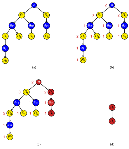
Figure 8: A generic execution of Algorithm 1.

Proposition 2

Given a ground ASP program $\Pi$, an answer set $X$ for $\Pi$, and an atom $p$ in $X$, Algorithm 1 terminates.

Proposition 3

Given a ground ASP program $\Pi$, an answer set $X$ for $\Pi$, and an atom $p$ in $X$, Algorithm 1 either finds a shortest explanation for $p$ with respect to $\Pi$ and $X$ or returns an empty vertex-labeled tree.

Proposition 4

Given a ground ASP program $\Pi$, an answer set $X$ for $\Pi$, and an atom $p$ in $X$, the time complexity of Algorithm 1 is $O(|\Pi|^{|X|}\times|\mathcal{B}_{\Pi}|)$.

We generate the complete and-or explanation tree while finding a shortest explanation. In fact, we can find a shortest explanation by creating a partial and-or explanation tree using a branch-and-bound idea. In particular, the idea is to compute the weights of vertices during the creation of the and-or explanation tree and, in case there exists a branch of the and-or explanation tree that exceeds the weight of a vertex computed so far, to stop branching on unnecessary parts of the and-or explanation tree. Then, a shortest explanation can be extracted by the same method used previously, i.e., by traversing a subtree of the and-or explanation tree and ignoring the atom vertices in this subtree. For instance, consider Figure 8(b). Assume that we first create the right branch of the root. Since the weight of an atom vertex is equal to the minimum weight among its children weights, we know that the weight of the root is at most 2. Now, we check whether it is necessary to branch on the left child of the root. Note that the weight of a rule vertex is equal to 1 plus the sum of its children weights. As $R_{1}$ has two children, its weight is at least 3. Therefore, it is redundant to branch on the left child of the root. This improvement is not implemented and is a future work.

6 Generating $k$ Different Explanations

When there is more than one explanation for an answer of a query, it might be useful to provide the experts with several more explanations that are different from each other. For instance, consider the query Q5 in Table 1.

• What are the drugs that treat the disease Asthma or that react with the drug Epinephrine?

An answer for this query is “Doxepin”. According to one explanation, “Doxepin” reacts with “Epinephrine” with respect to DrugBank. At this point, the expert may not be convinced and ask for a different explanation. Another explanation for this answer is that “Doxepin” treats “Asthma” according to CTD. Motivated by this example, we study generating different explanations.

Input: $\Pi$: ground ASP program, $X$: answer set for $\Pi$, $p$: atom in $X$, $k:$ a positive integer. Assume there are $n$ different explanations for $p$ w.r.t $\Pi$ and $X$.

Output: $\hbox{min\/}\{n,k\}$ different explanations for $p$ with respect to $\Pi$ and $X$.

1 $K:=\emptyset$, $R_{0}:=\emptyset$;

2 $\left\langle V,E,l,\Pi,X\right\rangle:=\mbox{createTree}(\Pi,X,p,\{\})$;

3 $v\leftarrow$ root of $\left\langle V,E\right\rangle$;

4 for $i=1,2,\ldots k$ do

5       $\mbox{calculateDifference}(\Pi,X,V,l,v,E,R_{i-1},W_{T,R_{i-1}})$;

6       if $W_{T,R_{i-1}}(v)=0$ then  return $K$;

7       ;

8       $\left\langle V^{\prime},E^{\prime},l,\Pi,X\right\rangle:=\mbox{extractExp}(\Pi,X,V,l,v,E,W_{T,R_{i-1}},\emptyset,\hbox{max\/})$;

9       $K_{i}\leftarrow\left\langle V^{\prime},E^{\prime},l,\Pi,X\right\rangle$;

10       $K:=K\cup\{K_{i}\}$;

11       $R_{i}:=R_{i-1}\cup\{v\,|\,\mbox{rule vertex}\ v\in V^{\prime}\}$;

12      

13return $K$;

Algorithm 5 Generating $k$ Different Explanations

We introduce an algorithm (Algorithm 5) to compute $k$ different explanations for an atom $p$ in $X$ with respect to $\Pi$ and $X$. For that, we define a distance measure $\Delta_{D}$ between a set $Z$ of (previously computed) explanations, and an (to be computed) explanation $S$. We consider the rule vertices $R_{Z}$ and $R_{S}$ contained in $Z$ and $S$, respectively. Then, we define the function $\Delta_{D}$ that measures the distance between $Z$ and $S$ as follows:

$$\Delta_{D}(Z,S)=|R_{S}\backslash R_{Z}|.$$

In the following, we sometimes use $R_{Z}$ and $R_{S}$ instead of $Z$ and $S$ in $\Delta_{D}$. Also, we denote by $\hbox{RVertices\/}(S)$ the set of rule vertices of a vertex-labeled tree $S$.

Let us now explain Algorithm 5. It computes a set $K$ of $k$ different explanations iteratively. Initially, $K=\emptyset$. First, we compute the and-or explanation tree $T$ (Line $2$). Then, we enter into a loop that iterates at most $k$ times (Line $4$). At each iteration $i$, an explanation $K_{i}$ that is most distant from the previously computed $i-1$ explanations is extracted from $T$. Let us denote the rule vertices included in the previously computed $i-1$ explanations by $R_{i-1}$. Then, essentially, at each iteration we pick an explanation $K_{i}$ such that $\Delta_{D}(R_{i-1},\hbox{RVertices\/}(K_{i}))$ is maximum. To be able to find such a $K_{i}$, we need to define the “contribution” of each vertex $v$ in $T$ to the distance measure $\Delta_{D}(R_{i-1},\hbox{RVertices\/}(K_{i}))$ if $v$ is included in explanation $K_{i}$:

$$W_{T,R_{i-1}}(v)=\left\{\begin{array}[]{ll}\hbox{max\/}\{W_{T,R_{i-1}}(v^{\prime})\,|\,v^{\prime}\in\hbox{child\/}_{E}(v)\}&\mbox{if}\ v\ \mbox{is an atom vertex};\\ \sum_{v^{\prime}\in\hbox{child\/}_{E}(v)}W_{T,R_{i-1}}(v^{\prime})&\mbox{if}\ v\ \mbox{is a rule vertex and}\\ &v\in R_{i-1};\\ 1+\sum_{v^{\prime}\in\hbox{child\/}_{E}(v)}W_{T,R_{i-1}}(v^{\prime})&\mbox{otherwise}.\end{array}\right.$$

Note that this function is different from $W_{T}$. Intuitively, $v$ contributes to the distance measure if it is not included in $R_{i-1}$. The contributions of vertices in $T$ are computed by Algorithm 6 (Line $5$) by propagating the contributions up in the spirit of Algorithm 3. Then, $K_{i}$ is extracted from weighted-$T$ by using Algorithm 4 (Line $7$).

Input: $\Pi:$ ground ASP program, $X:$ answer set for $\Pi$, $V:$ set of vertices, $l:V\rightarrow\Pi\cup X$, $v:$ vertex in $V$, $E:$ set of edges, $R:$ set of rule vertices in $V$, $D_{R}:$ candidate distance function.

Output: distance of $v$.

1 if $l(v)\in X$ then

2       foreach $c\in\hbox{child\/}_{E}(v)$ do

3             $D_{R}(c):=\mbox{calculateDifference}(\Pi,X,V,l,c,E,R,D_{R})$;

4            

5      $D_{R}(v):=\hbox{max\/}\{D_{R}(c)\,|\,c\in\hbox{child\/}_{E}(v)\}$;

6      

7else if $l(v)\in\Pi$ then

8       if $v\notin R$ then  $D_{R}(v):=1$;

9       ;

10       else  $D_{R}(v):=0$;

11       ;

12      

13      foreach $c\in\hbox{child\/}_{E}(v)$ do

14             $D_{R}(v):=D_{R}(v)+\mbox{calculateDifference}(\Pi,X,V,l,c,E,R,D_{R})$;

15            

16      

17return $D_{R}(v)$;

Algorithm 6 calculateDifference

The execution of Algorithm 5 is also illustrated in Figure 9. Similar to Algorithm 1, which generates shortest explanations, first the and-or explanation tree is created, which has a generic structure as shown in Figure 9(a). Recall that yellow vertices denote atom vertices and blue vertices denote rule vertices. For the sake of example, assume that $R=\{R_{2},R_{6}\}$. Then, the goal is to generate an explanation that contains different rule vertices from the rule vertices in $R$ as much as possible. For that, the weights of vertices are assigned according to the weight function $W_{T,R}$ as depicted in Figure 9(b). Here, the weight of the root implies that there exists an explanation which contains $4$ different rule vertices from the rule vertices in $R$ and this explanation is the most different one. Then, starting from the root, a subtree of the and-or explanation tree is traversed by visiting maximum weighted child of every atom vertex, and every child of every rule vertex. This subtree is shown in Figure 9(c) by red vertices. Finally, an explanation is extracted by ignoring the atom vertices and keeping the parent-child relationship as it is, from this subtree. This explanation is illustrated in Figure 9(d).

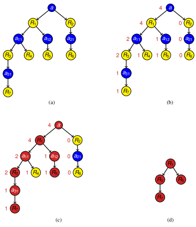
Figure 9: A generic execution of Algorithm 5.

Proposition 5

Given a ground ASP program $\Pi$, an answer set $X$ for $\Pi$, an atom $p$ in $X$, and a positive integer $k$, Algorithm 5 terminates.

Proposition 6

Let $\Pi$ be a ground ASP program, $X$ be an answer set for $\Pi$, $p$ be an atom in $X$, and $k$ be a positive integer. Let $n$ be the number of different explanations for $p$ with respect to $\Pi$ and $X$. Then, Algorithm 5 returns $\hbox{min\/}\{n,k\}$ different explanations for $p$ with respect to $\Pi$ and $X$.

Furthermore, at each iteration $i$ of the loop in Algorithm 5 the distance $\Delta_{D}(R_{i-1},K_{i})$ is maximized.

Proposition 7

Let $\Pi$ be a ground ASP program, $X$ be an answer set for $\Pi$, $p$ be an atom in $X$, and $k$ be a positive integer. Let $n$ be the number of explanations for $p$ with respect to $\Pi$ and $X$. Then, at the end of each iteration $i$ ($1\leq i\leq\hbox{min\/}\{n,k\}$) of the loop in Algorithm 5, $\Delta_{D}(R_{i-1},\hbox{RVertices\/}(K_{i}))$ is maximized, i.e., there is no other explanation $K^{\prime}$ such that $\Delta_{D}(R_{i-1},\hbox{RVertices\/}(K_{i}))<\Delta_{D}(R_{i-1},\hbox{RVertices\/}(K^{\prime}))$.

This result leads us to some useful consequences. First, Algorithm 5 computes “longest” explanations if $k=1$. The following corollary shows how to compute longest explanations.

Corollary 1

Let $\Pi$ be a ground ASP program, $X$ be an answer set for $\Pi$, $p$ be an atom in $X$, and $k=1$. Then, Algorithm 5 computes a longest explanation for $p$ with respect to $\Pi$ and $X$.

Next, we show that Algorithm 5 computes $k$ different explanations such that for every $i$ ($1\leq i\leq k$) the $i^{th}$ explanation is the most distant explanation from the previously computed $i-1$ explanations.

Corollary 2

Let $\Pi$ be a ground ASP program, $X$ be an answer set for $\Pi$, $p$ be an atom in $X$, and $k$ be a positive integer. Let $n$ be the number of explanations for $p$ with respect to $\Pi$ and $X$. Then, Algorithm 5 computes $\hbox{min\/}\{n,k\}$ different explanations $K_{1},\ldots,K_{\hbox{min\/}{\{n,k\}}}$ for $p$ with respect to $\Pi$ and $X$ such that for every $j$ ($2\leq j\leq\hbox{min\/}\{n,k\}$) $\Delta_{D}(\bigcup_{z=1}^{j-1}\hbox{RVertices\/}(K_{z}),K_{j})$ is maximized.

The following proposition shows that the time complexity of Algorithm 5 is exponential in the size of the given answer set.

Proposition 8

Given a ground ASP program $\Pi$, an answer set $X$ for $\Pi$, an atom $p$ in $X$ and a positive integer $k$, the time complexity of Algorithm 5 is $O(k\times|\Pi|^{|X|+1}\times|\mathcal{B}_{\Pi}|)$.

7 Experiments with Biomedical Queries

Our algorithms for generating explanations are applicable to the queries Q1, Q2, Q3, Q4, Q5, Q8, Q10, Q11 and Q12 in Table 1. The ASP programs for the other queries involve choice expressions. For instance, the query Q7 asks for cliques of 5 genes. We use the following rule to generate a possible set of 5 genes that might form a clique.

5{clique(GEN):gene_name(GEN)}5.

Our algorithms apply to ASP programs that contain a single atom in the heads of the rules, and negation and cardinality expressions in the bodies of the rules. Therefore, our methods are not applicable to the queries which are presented by ASP programs that include choice expressions.

Table 2: Experimental results for generating shortest explanations for some biomedical queries, using Algorithm 1.

Query	CPU Time	Explanation	Answer Set	And-Or Tree	gringo calls
		Size	Size	Size
Q1	52.78s	5	1.964.429	16	0
Q2	67.54s	7	2.087.219	233	1
Q3	31.15s	6	1.567.652	15	0
Q4	1245.83s	6	19.476.119	6690	4
Q5	41.75s	3	1.465.817	16	0
Q8	40.96s	14	1.060.288	28	4
Q10	1601.37s	14	1.612.128	3419	193
Q11	113.40s	6	2.158.684	5528	5
Q12	327.22s	5	10.338.474	10	1

In Table 2, we present the results for generating shortest explanations for the queries Q1, Q2, Q3, Q4, Q5, Q8, Q10, Q11 and Q12. In this table, the second column denotes the CPU timings to generate shortest explanations in seconds. The third column consists of the sizes of explanations, i.e., the number of rule vertices in an explanation. In the fourth column, the sizes of answer sets, i.e., the number of atoms in an answer set, are given. The fifth column presents the sizes of the and-or explanation trees, i.e., the number of vertices in the tree.

Before telling what the last column presents, let us clarify an issue regarding the computation of explanations. Since answer sets contain millions of atoms, the relevant ground programs are also huge. Thus, first grounding the programs and then generating explanations over those grounded programs is an overkill in terms of computational efficiency. To this end, we apply another method and do grounding when it is necessary. To better explain the idea, let us present our method by an example. At the beginning, we have a ground atom for which we are looking for shortest explanations. Assume that this atom is what_be_genes("ADRB1"). Then, we find the rules whose heads are of the form what_be_genes(GN), and instantiate $GN$ with “ADRB1”. For instance, assume that the following rule exists in the program:

$$\hbox{what\_be\_genes(GN)\/}\leftarrow\hbox{drug\_gene(DRG,GN)\/}$$

Then, by such an instantiation, we obtain the following instance of this rule:

$$\hbox{what\_be\_genes("ADRB1")\/}\leftarrow\hbox{drug\_gene(DRG,"ADRB1")\/}$$

Next, if the rules that we obtain by instantiating their heads are not ground, we ground them using the grounder gringo considering the answer set. We apply the same method for the atoms that are now ground, to find the relevant rules and ground them if necessary. This allows us to deal with a relevant subset of the rules while generating explanations. The last column of Table 2 presents the number of times gringo is called for such incremental grounding. For instance, for the queries Q1, Q3 and Q5, gringo is never called. However, gringo is called 193 times during the computation of a shortest explanation for the query Q10.

As seen from the results presented in Table 2, the computation time is not very much related to the size of the explanation. As also suggested by the complexity results of Algorithm 1 (i.e., $O(|\Pi|^{|X|}\times|\mathcal{B}_{\Pi})|$), the computation time for generating shortest explanations greatly depends on the sizes of the answer set and the and-or explanation tree. For instance, for the query Q4, the answer set contains approximately 19 million atoms, the size of the and-or explanation tree is 6690, and it takes 1245 CPU seconds to compute a shortest explanation, whereas for the query Q8, the answer set approximately contains 1 million atoms, the and-or explanation tree has 28 vertices, and it takes 40 CPU seconds to compute a shortest explanation. Also, the number of times gringo is called during the computation affects the computation time. For instance, for the query Q10 the answer set approximately contains 1.6 million atoms, the and-or explanation tree has 3419 vertices, and it takes 1600 CPU seconds to compute a shortest explanation.

Table 3 shows the computation times for generating different explanations for the answers of the same queries, if exists. As seen from these results, the time for computing 2 and 4 different explanations is slightly different than the time for computing shortest explanations.

Table 3: Experimental results for generating different explanations for some biomedical queries, using Algorithm 5.

Query	CPU Time
	$2$ different	$4$ different	Shortest
Q1	53.73s	-	52.78s
Q2	66.88s	67.15s	67.54s
Q3	31.22s	-	31.15s
Q4	1248.15s	1251.13s	1245.83s
Q5	-	-	41.75s
Q8	-	-	40.96s
Q10	1600.49s	1602.16s	1601.37s
Q11	113.25s	112.83s	113.40s
Q12	-	-	327.22s

8 Presenting Explanations in a Natural Language

An explanation for an answer of a biomedical query may not be easy to understand, since the user may not know the syntax of ASP rules neither the meanings of predicates. To this end, it is better to present explanations to the experts in a natural language.

Observe that leaves of an explanation denote facts extracted from the biomedical resources. Also some internal vertices contain informative explanations such as the position of a drug in a chain of drug-drug interactions. Therefore, there is a corresponding natural language explanation for some vertices in the tree. Such a correspondence can be stored in a predicate look-up table, like Table 4. Given such a look-up table, a pre-order depth-first traversal of an explanation and generating natural language expressions corresponding to vertices of the explanation lead to an explanation in natural language [Oztok (2012)].

For instance, the explanation in Figure 6 is expressed in natural language as illustrated in the introduction.

Table 4: Predicate look-up table used while expressing explanations in natural language.

Predicate	Expression in Natural Language
gene_gene_biogrid(x,y)	The gene x interacts with the gene y according to BioGRID.
drug_disease_ctd(x,y)	The disease y is treated by the drug x according to CTD.
drug_gene_ctd(x,y)	The drug x targets the gene y according to CTD.
gene_disease_ctd(x,y)	The disease y is related to the gene x according to CTD.
disease_symptom_do(x,y)	The disease x has the symptom y according to Disease Ontology.
drug_category_drugbank(x,y)	The drug x belongs to the category y according to DrugBank.
drug_drug_drugbank(x,y)	The drug x reacts with the drug y according to DrugBank.
drug_sideeffect_sider(x,y)	The drug x has the side effect y according to SIDER.
disease_gene_orphadata(x,y)	The disease x is related to the gene y according to Orphadata.
drug_disease_pharmgkb(x,y)	The disease y is treated by the drug x according to PharmGKB.
drug_gene_pharmgkb(x,y)	The drug x targets the gene y according to PharmGKB.
disease_gene_pharmgkb(x,y)	The disease x is related to the gene y according to PharmGKB.
start_drug(x)	The drug x is the start drug.
start_gene(x)	The gene x is the start gene.
$\hbox{drug\_reachable\_from\/}(x,l)$	The distance of the drug x from the start drug is l.
$\hbox{gene\_reachable\_from\/}(x,l)$	The distance of the gene x from the start gene is l.

9 Implementation of Explanation Generation Algorithms

Based on the algorithms introduced above, we have developed a computational tool called ExpGen-ASP [Oztok (2012)], using the programming language C++. Given an ASP program and its answer set, ExpGen-ASP generates shortest explanations as well as $k$ different explanations.

The input of ExpGen-ASP are

• an ASP program $\Pi$,

• an answer set $X$ for $\Pi$,

• an atom $p$ in $X$,

• an option that is used to generate either a shortest explanation or $k$ different explanations,

• a predicate look-up table,

and the output are

• a shortest explanation for $p$ with respect to $\Pi$ and $X$ in a natural language (if shortest explanation option is chosen),

• $k$ different explanations for $p$ with respect to $\Pi$ and $X$ in a natural language (if $k$ different explanations option is chosen).

For generating shortest explanations (resp., $k$ different explanations), ExpGen-ASP utilizes Algorithm 1 (resp., Algorithm 5).

To provide experts with further informative explanations about the answers of biomedical queries, we have embedded ExpGen-ASP into BioQuery-ASP by utilizing Table 4 as the predicate look-up table of the system. Figure 10 shows a snapshot of the explanation generation mechanism of BioQuery-ASP.

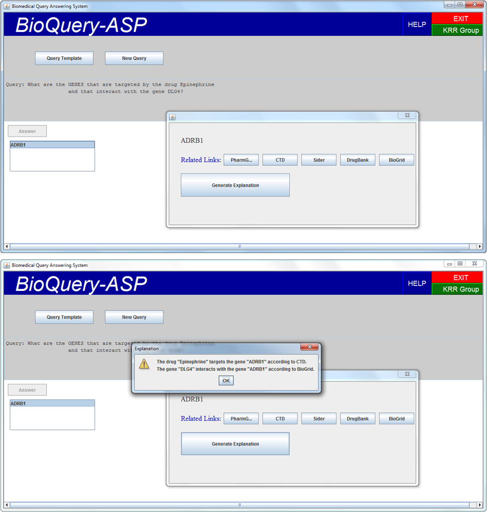
Figure 10: A snapshot of BioQuery-ASP showing its explanation generation facility.

10 Relating Explanations to Justifications

The most similar work to ours is [Pontelli et al. (2009)] that study the question “why is an atom $p$ in an answer set $X$ for an ASP program $\Pi$”. As an answer to this question, the authors of [Pontelli et al. (2009)] finds a “justification”, which is a labeled graph that provides an explanation for the truth values of atoms with respect to an answer set.

Example 6

Let $\Pi$ be the program presented in Example 1:

$$\begin{array}[]{l}a\leftarrow b,c\\ a\leftarrow d\\ d\leftarrow\\ b\leftarrow c\\ c\leftarrow\end{array}$$

and $X=~{}\{a,b,c,d\}$. Figure 11 is an offline justification of $a^{+}$ with respect to $X$ and $\emptyset$. Intuitively, $a$ is in $X$ since $b$ and $c$ are also in $X$ and there is a rule in $\Pi$ that supports $a$ using the atoms $b$ and $c$. Furthermore, $b$ is in $X$ since $c$ is in $X$ and there is a rule in $\Pi$ that supports $b$ using the atom $c$. Finally, $c$ is in $X$ as it is a fact in $\Pi$.

Figure 11: An offline justification for Example 6.

To relate offline justifications and explanations, we need to introduce the following definitions and notations about justifications defined in [Pontelli et al. (2009)].

10.1 Offline Justifications

First, let us introduce notations related to ASP programs used in [Pontelli et al. (2009)]. The class of ASP programs studied is normal programs, i.e., programs that consist of the rules of the form

$$A\leftarrow A_{1},\ldots,A_{k},not\ A_{k+1},\ldots,not\ A_{m}$$

where $m\geq k\geq 0$ and $A$ and each $A_{i}$ is an atom. Therefore, the programs we consider are more general. Let $\Pi$ be a normal ASP program. Then, $\mathcal{A}_{\Pi}$ is the Herbrand base of $\Pi$. An interpretation $I$ for a program $\Pi$ is defined as a pair $\left\langle I^{+},I^{-}\right\rangle$, where $I^{+}\cup I^{-}\subseteq\mathcal{A}_{\Pi}$ and $I^{+}\cap I^{-}=\emptyset$. Intuitively, $I^{+}$ denotes the set of atoms that are true, while $I^{-}$ denotes the set of atoms that are false. $I$ is a complete interpretation if $I^{+}\cup I^{-}=\mathcal{A}_{\Pi}$. The reduct $\Pi^{I}$ of $\Pi$ with respect to $I$ is defined as

$$\Pi^{I}=\{H(r)\leftarrow B^{+}(r)\,|\,r\in\Pi,\,B^{-}(r)\cap I^{+}=\emptyset\}$$

A complete interpretation $M$ for a program $\Pi$ is an answer set for $\Pi$ if $M^{+}$ is an answer set for $\Pi^{M}$. Also, a literal is either an atom or a formula of the form $not\ a$ where $a$ is an atom. The set of atoms which appear as negated literals in $\Pi$ is denoted by $NANT(\Pi)$. For an atom $a$, $a^{+}$ denotes that the atom $a$ is true and $a^{-}$ denotes that $a^{-}$ is false. Then, $a^{+}$ and $a^{-}$ are called the annotated versions of $a$. Moreover, it is defined that $atom(a^{+})=a$ and $atom(a^{-})=a$. For a set $S$ of atoms, the following sets of annotated atoms are defined.

• $S^{p}=\{a^{+}\,|\,a\in S\}$

• $S^{n}=\{a^{-}\,|\,a\in S\}$

Finally, the set $not\ S$ is defined as $not\ S=\{not\ a\,|\,a\in S\}$.

Apart from the answer set semantics, there is another important semantics of logic programs, called the well-founded semantics [Gelder et al. (1991)]. Since this semantics is important to build the notion of a justification, we now briefly describe the well-founded semantics. We consider the definition proposed in [Apt and Bol (1994)], instead of the original definition proposed in [Gelder et al. (1991)], as the authors of [Pontelli et al. (2009)] considered.

Definition 7 (Immediate consequence)

Let $\Pi$ be a normal ASP program, and $S$ and $V$ be two sets of atoms from $\mathcal{A}_{\Pi}$. Then, the immediate consequence of $S$ with respect to $\Pi$ and $V$, denoted by $T_{\Pi,V}(S)$ is the set defined as follows:

$$T_{\Pi,V}(S)=\{a\,|\,\exists\ r\in\Pi,\,H(r)=a,\,B^{+}(r)\subseteq S,\,B^{-}(r)\cap V=\emptyset\}.$$

We denote by $lfp(T_{\Pi,V})$ the least fixpoint of $T_{\Pi,V}$ when $V$ is fixed.

Definition 8 (The well-founded model)

Let $\Pi$ be a normal ASP program, $\Pi^{+}=\{r\,|\,r\in\Pi,\,B^{-}(r)=\emptyset\}$. The sequence $\left\langle K_{i},U_{i}\right\rangle_{i\geq 0}$ is defined as follows:

$$\begin{array}[]{l l l}K_{0}=lfp(T_{\Pi^{+}}),&&U_{0}=lfp(T_{\Pi,K_{0}}),\\ K_{i}=lfp(T_{\Pi,U_{i-1}}),&&U_{i}=lfp(T_{\Pi,K_{i}}).\\ \end{array}$$

Let $j$ be the first index of the computation such that $\left\langle K_{j},U_{j}\right\rangle=\left\langle K_{j+1},U_{j+1}\right\rangle$. Then, the well-founded model of $\Pi$ is $WF_{\Pi}=\left\langle W^{+},W^{-}\right\rangle$ where $W^{+}=K_{j}$ and $W^{-}=\mathcal{A}_{\Pi}\backslash U_{j}$.

Example 7

Let $\Pi$ be the program

$$\begin{array}[]{l}a\leftarrow b,not\ d\\ d\leftarrow b,not\ a\\ b\leftarrow c\\ c\leftarrow\end{array}$$

Then, the well-founded model of $\Pi$ is computed as follows:

$$K_{0} = \{b,c\},$$

$$U_{0} = \{a,b,c,d\},$$

$$K_{1} = \{b,c\},$$

$$U_{0} = \{a,b,c,d\}.$$

Thus, $WF_{\Pi}=\left\langle\{b,c\},\emptyset\right\rangle$.

We now provide definitions regarding the notion of an offline justification. First, we introduce the basic building of an offline justification, a labeled graph called as e-graph.

Definition 9 (e-graph)

Let $\Pi$ be a normal ASP program. An e-graph for $\Pi$ is a labeled, directed graph $(N,E)$, where $N\subseteq\mathcal{A}_{\Pi}^{p}\cup\mathcal{A}_{\Pi}^{n}\cup\{assume,\top,\bot\}$ and $E\subseteq N\times N\times\{+,-\}$, which satisfies following properties:

• the only sinks (i.e., nodes without out-going edges) in the graph are $assume,\top,\bot$;

• for every $b\in N\cap\mathcal{A}_{\Pi}^{p}$, $(b,assume,-)\notin E$ and $(b,\bot,-)\notin E$;

• for every $b\in N\cap\mathcal{A}_{\Pi}^{n}$, $(b,assume,+)\notin E$ and $(b,\top,+)\notin E$;

• for every $b\in N$, if for some $l\in\{assume,\top,\bot\}$ and $s\in\{+,-\}$, $(b,l,s)\in E$, then $(b,l,s)$ is the only out-going edge originating from $b$.

According to this definition, an edge of an e-graph connects two annotated atoms or an annotated atom with one of the nodes in $\{assume,\top,\bot\}$ and is marked by a label from $\{+,-\}$. An edge is called as positive (resp., negative) if it is labeled by $+$ (resp., $-$). Also, a path in an e-graph is called as positive if it has only positive edges, whereas it is called as negative if it has at least one negative edge. The existence of a positive path between two nodes $v_{1}$ and $v_{2}$ is denoted by $(v_{1},v_{2})\in E^{*,+}$. In the offline justification, $\top$ is used to explain facts, $\bot$ to explain atoms which do not have defining rules, and $assume$ is for atoms for which explanations are not needed, i.e., they are assumed to be true or false.

Example 8

Let $\Pi$ be the program presented in Example 1, and $X=~{}\{a,b,c,d\}$. Then, Figure 12 is an e-graph for $\Pi$. Intuitively, the true state of $a$ depends on the true state of $b$ and the false state of $c$, where $b$ is assumed to be true and $c$ is assumed to be false.

Figure 12: An e-graph for Example 8.

In an e-graph, a set of elements that directly contributes to the truth value of an atom can be obtained through the out-going edges of a corresponding node. This set is defined as follows.

Definition 10 ($support(b,G)$)

Let $\Pi$ be a normal ASP program, $G=(N,E)$ be an e-graph for $\Pi$ and $b\in N\cap(\mathcal{A}_{\Pi}^{p}\cup\mathcal{A}_{\Pi}^{n})$ be a node in $G$. Then, $support(b,G)$ is defined as follows.

• $support(b,G)=\{l\}$, if for some $l\in\{assume,\top,\bot\}$ and $s\in\{+,-\}$, $(b,l,s)$ is in $E$;

• $support(b,G)=\{atom(c)\,|\,(b,c,+)\in E\}\cup\{not\,atom(c)\,|\,(b,c,-)\in E\}$, otherwise.

Example 9

Let $G$ be the e-graph in Figure 12. Then, $support(a,G)=\{b,not\ c\}$, $support(b,G)=\{assume\}$ and $support(c,G)=\{assume\}$.

To define the notion of a justification, an e-graph should be enriched with explanations of truth values of atoms that are derived from the rules of the program. For that, the concept of one step justification of a literal is defined as follows.

Definition 11 (Local Consistent Explanation (LCE))

Let $\Pi$ be a normal ASP program, $b$ be an atom, $J$ be a possible interpretation for $\Pi$, $U\subseteq\mathcal{A}_{\Pi}$ be a set of atoms, and $S\subseteq\mathcal{A}_{\Pi}\cup\mbox{not}\,\mathcal{A}_{\Pi}\cup\{assume,\top,\bot\}$ be a set of literals. We say that

• $S$ is an LCE of $b^{+}$ with respect to $(J,U)$, if $b\in J^{+}$ and

  • $S=\{assume\}$ or

  • $S\cap\mathcal{A}_{\Pi}\subseteq J^{+}$, $\{c\,|\,\mbox{not}\,c\in S\}\subseteq J^{-}\cup U$, and there is a rule $r\in\Pi$ such that $H(r)=b$ and $B(r)=S$. In case, $B(r)=\emptyset$, $S$ is denoted by the set $\{\top\}$.

• $S$ is an LCE of $b^{-}$ with respect to $(J,U)$, if $b\in J^{-}\cup U$ and

  • $S=\{assume\}$ or

  • $S\cap\mathcal{A}\subseteq J^{-}\cup U$, $\{c\,|\,not\,c\in S\}\subseteq J^{+}$, and $S$ is a minimal set of literals such that for every rule $r\in\Pi$ if $H(r)=b$, then $B^{+}(r)\cap S\neq\emptyset$ or $B^{-}(r)\cap\{c\,|\,\mbox{not}\,c\in S\}\neq\emptyset$. In case, $S=\emptyset$, $S$ is denoted by the set $\{\bot\}$.

The set of all the LCEs of $b^{+}$ with respect to $(J,U)$ is denoted by $\mbox{LCE}_{\Pi}^{p}(b,J,U)$ and the set of all the LCEs of $b^{-}$ with respect to $(J,U)$ is denoted by $\mbox{LCE}_{\Pi}^{n}(b,J,U)$.

Here, a possible interpretation $J$ denotes an answer set. The set $U$ consists of atoms that are assumed to be false (which will be called as Assumptions in the notion of justification later on). The need for $U$ comes from the fact that the truth value of some atoms is first guessed while computing answer sets. Intuitively, if an atom $a$ is true, an LCE consists of the body of a rule which is satisfied by $J$ and has $a$ in its head; if $a$ is false, an LCE consists of a set of literals that are false in $J$ and falsify all rules whose head are $a$.

Example 10

Let $\Pi$ and $X$ be defined as in Example 8. Then, the LCEs of the atoms with respect to $(X,\emptyset)$ is as follows.

$$\mbox{LCE}_{\Pi}^{p}(a,X,\emptyset) = \{\{b,c\},\{d\},\{assume\}\}$$

$$\mbox{LCE}_{\Pi}^{p}(b,X,\emptyset) = \{\{c\},\{assume\}\}$$

$$\mbox{LCE}_{\Pi}^{p}(c,X,\emptyset) = \{\{\top\},\{assume\}\}$$

$$\mbox{LCE}_{\Pi}^{p}(d,X,\emptyset) = \{\{\top\},\{assume\}\}$$

Accordingly, a class of e-graphs where edges represent LCEs of the corresponding nodes are defined as follows.

Definition 12 ($(J,U)$-based e-graph)

Let $\Pi$ be a normal ASP program, $J$ be a possible interpretation for $\Pi$, $U\subseteq\mathcal{A}_{\Pi}$ be a set of atoms and $b$ be an element in $\mathcal{A}_{\Pi}^{p}\cup\mathcal{A}_{\Pi}^{n}$. A $(J,U)$-based e-graph $G=(N,E)$ of $b$ is an e-graph such that

• every node $c\in N$ is reachable from $b$,

• for every $c\in N\backslash\{assume,\top,\bot\}$, $support(c,G)$ is an LCE of $c$ with respect to $(J,U)$;

A $(J,U)$-based e-graph $(N,E)$ is safe if for all $b^{+}\in N,(b^{+},b^{+})\notin E^{*,+}$, i.e., there is no positive cycle in the graph.

We now introduce a special class of $(J,U)$-based e-graphs where only false elements can be assumed.

Definition 13 (Offline e-graph)

Let $\Pi$ be a normal ASP program, $J$ be a partial interpretation for $\Pi$, $U\subseteq\mathcal{A}_{\Pi}$ be a set of atoms and $b$ be an element in $\mathcal{A}^{p}\cup\mathcal{A}^{n}$. An offline e-graph $G=(N,E)$ of $b$ with respect to $J$ and $U$ is a $(J,U)$-based e-graph of $b$ that satisfies following properties:

• there exists no $p^{+}\in N$ such that $(p^{+},assume,+)\in E$;

• $(p^{-},assume,-)\in E$ if and only if $p\in U$.

$\mathcal{E}(b,J,U)$ is the set of all offline e-graphs of $b$ with respect to $J$ and $U$.

Here, the roles of $J$ and $U$ are the same as their roles in Definition 11. Observe that true atoms cannot be assumed due to the first condition and only elements in the set $U$ are assumed due to the second condition.

We said earlier that in a $(J,U)$-based e-graph $J$ represents an answer set and $U$ consists of atoms that are assumed to be false. Here, $U$ is chosen based on some characteristics of $J$. In particular, we want $U$ to be a set of atoms such that when its elements are assumed to be false, the truth value of other atoms in the program can be uniquely determined and leads to $J$. We now introduce regarding definitions formally.

Definition 14 (Tentative Assumptions)

Let $\Pi$ be a normal ASP program, $M$ be an answer set for $\Pi$ and $WF_{\Pi}=<WF^{+}_{\Pi},WF^{-}_{\Pi}>$ be the well-founded model of $\Pi$. The tentative assumptions $\mathcal{TA}_{\Pi}(M)$ of $\Pi$ with respect to $M$ are defined as

$$\mathcal{TA}_{\Pi}(M)=\{a\,|\,a\in NANT(\Pi)\wedge a\in M^{-},a\notin(WF^{+}_{\Pi}\cup WF^{-}_{\Pi})\}$$ (9)

Example 11

Let $\Pi$ be the program:

$$\begin{array}[]{l}c\leftarrow a,not\ d\\ d\leftarrow a,not\ c\\ a\leftarrow b\\ b\leftarrow\end{array}$$

Then, $X=\{a,b,c\}$ is an answer set for $\Pi$ and $\left\langle\{a,b\},\emptyset\right\rangle$ is the well-founded model of $\Pi$. Given that, $\mathcal{TA}_{\Pi}(X)=\{d\}$ as $d\in NANT(\Pi)$, $d\notin X$ and $d\notin(WF^{+}_{\Pi}\cup WF^{-}_{\Pi})$.

In fact, tentative assumptions is a set of atoms whose subsets might “potentially” form $U$.

We provide a definition that would allow one to obtain a program from a given program $\Pi$ and a set $V$ of atoms by assuming all the atoms in $V$ as false.

Definition 15 (Negative Reduct)

Let $\Pi$ be a normal ASP program, $M$ be an answer set for $\Pi$, and $U\subseteq\mathcal{TA}_{\Pi}(M)$ be a set of tentative assumption atoms. The negative reduct $NR(\Pi,U)$ of $\Pi$ with respect to $U$ is the set of rules defined as

$$NR(\Pi,U)=\Pi\backslash\{r\,|\,H(r)\in U\}$$ (10)

Finally, the concept of assumptions can be introduced formally.

Definition 16 (Assumption)

Let $\Pi$ be a normal ASP program, $M$ be an answer set for $\Pi$. An assumption of $\Pi$ with respect to $M$ is a set $U$ of atoms that satisfies the following properties:

• $U\subseteq\mathcal{TA}_{\Pi}(M)$;

• the well-founded model of $NR(\Pi,U)$ is equal to $M$.

$Assumptions(\Pi,M)$ is the set of all assumptions of $\Pi$ with respect to $M$.

Example 12

Let $\Pi$ and $X$ be defined as in Example 11. Let $U=\{d\}$. Then, $NR(\Pi,U)$ is:

$$\begin{array}[]{l}c\leftarrow a,not\ d\\ a\leftarrow b\\ b\leftarrow\end{array}$$

and $\left\langle\{a,b,c\},\emptyset\right\rangle$ is the well-founded model of $NR(\Pi,U)$. Thus, $U$ is an assumption of $\Pi$ with respect to $X$.

Note that assumptions are nothing but subsets of tentative assumptions that would allow to obtain the answer set $J$.

At last, we are ready to define the notion of offline justification.

Definition 17 (Offline Justification)

Let $\Pi$ be a normal ASP program, $M$ be an answer set for $\Pi$, $U$ be an assumption in $Assumptions(\Pi,M)$ and $b$ be an annotated atom in $\mathcal{A}^{p}\cup\mathcal{A}^{n}$. An offline justification of $b$ with respect to $M$ and $U$ is an element $(N,E)$ of $\mathcal{E}(b,M,U)$ which is safe.

According to the definition, a justification is a $(J,U)$-based e-graph where $J$ is an answer set and $U$ is an assumption. Also, justifications do not allow the creation of positive cycles in the justification of true atoms. For instance, for $\Pi$ and $X$ defined as in Example 1, Figure 11 illustrates an offline justification of $a^{+}$ with respect to $X$ and $\emptyset$.

In [Pontelli et al. (2009)], the authors prove the following proposition which shows that for every atom in the program, there exists an offline justification.

Proposition 9

Let $\Pi$ be a ground normal ASP program, $X$ be an answer for $\Pi$. Then, for each atom $a$ in $\Pi$, there is an offline justification of with respect to $X$ and $X^{-}\backslash WF_{\Pi}^{-}$ which does not contain negative cycles.

10.2 From Justifications to Explanations

We relate a justification to an explanation. In particular, given an offline justification, we show that one can obtain an explanation tree whose atom vertices are formed by utilizing the “annotated atoms” of the justification and rule vertices are formed by utilizing the “support” of annotated atoms. To compute such explanation trees, we develop Algorithm 7.

Input: $\Pi:$ ground normal ASP program, $X:$ answer set for $\Pi$, $p:$ atom in $X$, $(V,E):$ justification of $p^{+}$ w.r.t $X$ and some $U\in Assumptions(\Pi,X)$.

Output: A vertex-labeled tree $\left\langle V^{\prime},E^{\prime},l,\Pi,X\right\rangle$.

1 $V^{\prime}:=\emptyset,\,E^{\prime}:=\emptyset$;

2 $v\leftarrow$ Create a vertex $v$ s.t. $l(v)=p$;

3 $Q\leftarrow v$;

4 while $Q\neq\emptyset$ do

5       $v^{\prime}\leftarrow$ Dequeue an element from $Q$;

6       $V^{\prime}:=V^{\prime}\cup\{v^{\prime}\}$;

7       if $l(v^{\prime})\in\Pi$ then // $v^{\prime}$ is a rule vertex

8             foreach $a\in B^{+}(l(v^{\prime}))$ do

9                   $v^{\prime\prime}\leftarrow$ Create a vertex $v^{\prime\prime}$ s.t. $l(v^{\prime\prime})=a$;

10                   $E^{\prime}:=E^{\prime}\cup\{(v^{\prime},v^{\prime\prime})\}$ // edge from rule vertex to atom vertex ;

11                   Enqueue $v^{\prime\prime}$ to $Q$;

12                  

13            

14      

15      else if $l(v^{\prime})\in X$ then // $v^{\prime}$ is an atom vertex

16             $r\leftarrow$ Create a rule $r$ s.t. $H(r)=l(v^{\prime})$ and $B(r)=support(l(v^{\prime})^{+},G)$;

17             $v^{\prime\prime}\leftarrow$ Create a vertex $v^{\prime\prime}$ s.t. $l(v^{\prime\prime})=r$;

18             $E^{\prime}:=E^{\prime}\cup\{(v^{\prime},v^{\prime\prime})\}$ // edge from atom vertex to rule vertex ;

19             Enqueue $v^{\prime\prime}$ to $Q$;

20            

21      

22return $\left\langle V^{\prime},E^{\prime},l,\Pi,X\right\rangle$;

Algorithm 7 Justification to Explanation

Let us now explain the algorithm in detail. Algorithm 7 takes as input a ground normal ASP program $\Pi$ , an answer set $X$ for $\Pi$, an atom $p$ in $X$, and a justification $(V,E)$ of $p^{+}$ with respect to $X$ and some $U\in Assumptions(\Pi,X)$. Our goal is to obtain an explanation tree in the and-or explanation tree for $p$ with respect to $\Pi$ and $X$ from the justification $(V,E)$. The algorithm starts by creating two sets $V^{\prime}$ and $E^{\prime}$ (Line $1$). Here, $V^{\prime}$ and $E^{\prime}$ corresponds to the set of vertices and the set of edges of the explanation tree, respectively. By Condition $(ii)$ in Definition 3 and Condition $(i)$ in Definition 2, we know that the label of the root of an explanation tree for $p$ with respect to $\Pi$ and $X$ is $p$. Thus, a vertex $v$ with label $p$ is defined (Line $2$), and added into the queue $Q$ (Line $3$). Then, the algorithm enters into a “while” loop which executes until $Q$ becomes empty. At every iteration of the loop, an element $v$ from $Q$ is first extracted (Line $5$) and added into $V^{\prime}$ (Line $6$). This implies that every element added into $Q$ is also added into $V^{\prime}$. For instance, the vertex defined at Line $2$ is the first vertex extracted from $Q$ and also added into $V^{\prime}$, which makes sense since we know that the root of an explanation tree is an atom vertex with label $v$. Then, according to the type of the extracted vertex, its out-going edges are defined. Let $v^{\prime}$ be a vertex extracted from $Q$ at Line $5$ in some iteration of the loop. Consider the following two cases.

• Assume that $v^{\prime}$ is an atom vertex. Then, the algorithm directly goes to Line $13$. By Condition $(i)$ in Definition 3, we know that an explanation tree is a subtree of the and-or explanation tree. Hence, we need to define out-going edges of $v^{\prime}$ by taking into account Condition $(ii)$ in Definition 2, which implies that a child of $v^{\prime}$ must be a rule vertex $v^{\prime\prime}$ such that the rule that labels $v^{\prime\prime}$ “supports” the atom that labels $v^{\prime}$. Thus, a rule $r$ that supports the atom that labels $v^{\prime}$ is created (Line $13$). We ensure “supportedness” property by utilizing the annotated atoms in the given offline justification which supports the annotated version of the atom that labels $v^{\prime}$. Then, a vertex $v^{\prime\prime}$ with label $r$ is created (Line $14$), and a corresponding child of $v^{\prime}$ is added into $E^{\prime}$ (Line $15$). By Condition $(iii)$ in Definition 3, we know that every atom vertex of an explanation tree has a single child. Therefore, another child of $v^{\prime}$ is not created. Then, before finishing the iteration of the loop, the child $v^{\prime\prime}$ of $v^{\prime}$ is added into $Q$ so that its children can be formed in the next iterations of the loop.

• Assume that $v^{\prime}$ is a rule vertex. Then, the condition at Line $7$ is satisfied and the algorithm goes to Line $8$. In this case, while forming the children of $v^{\prime}$, we should consider Condition $(iii)$ in Definition 2, which implies that a child $v^{\prime\prime}$ of $v^{\prime}$ must be an atom vertex such that the atom that labels $v^{\prime\prime}$ is in the positive body of the rule that labels $v^{\prime}$. Also, by Condition $(iv)$ in Definition 3, we should ensure that for every atom $a$ in the positive body of the rule that labels $v^{\prime}$, there exists a child $v_{a}$ of $v^{\prime}$ such that the atom that labels $v_{a}$ is equal to $a$. Thus, the loop between Lines $8$–$11$ iterates for every atom $a$ in the positive body of the label of $v^{\prime}$ and a vertex $v^{\prime\prime}$ with label $a$ is created (Line $9$). Then, $v^{\prime\prime}$ becomes a child of $v^{\prime}$ (Line $10$). To form the children of $v^{\prime\prime}$ in the next iterations of the “while” loop, the child $v^{\prime\prime}$ of $v^{\prime}$ is added into $Q$ (Line $11$).

When the algorithm finishes processing the elements of $Q$, i.e., $Q$ becomes empty, the “while” loop terminates. Then, the algorithm returns a vertex-labeled tree (Line $17$). We now provide the proposition about the soundness of Algorithm 7.

Proposition 10

Given a ground normal ASP program $\Pi$, an answer set $X$ for $\Pi$, an atom $p$ in $X$, an assumption $U$ in $Assumption(\Pi,X)$, and an offline justification $G=(V,E)$ of $p^{+}$ with respect to $X$ and $U$, Algorithm 7 returns an explanation tree $\left\langle V^{\prime},E^{\prime},l,\Pi,X\right\rangle$ in the and-or explanation tree for $p$ with respect to $\Pi$ and $X$.

Example 13

Let $\Pi$ and $X$ be defined as in Example 8. Figure 13(a) is an offline justification of $a^{+}$ with respect to $X$ and $\emptyset$. Figure 13(b) shows a corresponding explanation tree in the and-or explanation tree for $a$ with respect to $\Pi$ and $X$ that is obtained by using Algorithm 7.

(a)

(b)

Figure 13: (a) An offline justification and (b) its corresponding explanation tree obtained by using Algorithm 7.

10.3 From Explanations to Justifications

We relate an explanation to a justification. In particular, given an explanation tree whose labels of vertices are unique, we show that one can obtain an offline justification by utilizing the labels of atom vertices of the explanation tree. For that, we design Algorithm 8.

Input: $\Pi:$ ground normal ASP program, $X:$ answer set for $\Pi$, $p:$ atom in $X$, $\left\langle V^{\prime},E^{\prime},l,\Pi,X\right\rangle:$ an explanation tree in the and-or explanation tree for $p$ w.r.t $\Pi$ and $X$.

Output: $(V,E):$ justification of $p^{+}$ w.r.t $X$ and $\emptyset$.

1 $V:=\emptyset,\,E:=\emptyset$;

2 $Q\leftarrow$ root of $\left\langle V^{\prime},E^{\prime}\right\rangle$;

3 while $Q\neq\emptyset$ do

4       $v\leftarrow$ Dequeue an element from $Q$;

5       $V:=V\cup\{l(v)^{+}\}$;

6       $v^{\prime}\leftarrow$ child of $v$ in $\left\langle V^{\prime},E^{\prime}\right\rangle$;

7       if $l(v^{\prime})$ is a fact in $\Pi^{X}$ then

8             $E:=E\cup\{(l(v)^{+},\top,+)\}$;

9            

10      foreach $v^{\prime\prime}\in\hbox{child\/}_{E^{\prime}}(v^{\prime})$ do

11             $E:=E\cup\{(l(v)^{+},l(v^{\prime\prime})^{+},+)\}$;

12             Enqueue $v^{\prime\prime}$ to $Q$;

13            

14      

15$V:=V\cup\{\top\}$;

16 return $(V,E)$;

Algorithm 8 Explanation to Justification

Let us now describe the algorithm in detail. Algorithm 8 takes as input a ground normal ASP program $\Pi$, an answer set $X$ for $\Pi$, an atom $p$ in $X$, and an explanation tree $T^{\prime}=\left\langle V^{\prime},E^{\prime},l,\Pi,X\right\rangle$ in the and-or explanation tree for $p$ with respect to $\Pi$ and $X$. Our goal is to obtain an offline justification $(V,E)$ of $p^{+}$ in $\Pi^{X}$ with respect to $X$ and $\emptyset$. The reason to obtain the offline justification in the reduct of $\Pi$ with respect to $X$ is that our definition of explanation is not defined for the atoms that are not in the answer set. Algorithm 8 starts by creating two sets $V$ and $E$ which will correspond to the set of nodes and the set of edges of the offline justification, respectively (Line $1$). Then, the root of $\left\langle V^{\prime},E^{\prime}\right\rangle$ is added into the queue $Q$ (Line $2$) and we enter into a “while” loop that iterates until $Q$ becomes empty. At every iteration of the loop, first an element $v$ is extracted from $Q$ (Line $4$) and $l(v)^{+}$ is added into $V$ (Line $5$). Then, we form the out-going edges of $l(v)^{+}$. Due to Condition $(iii)$ in Definition 3, every atom vertex in an explanation tree has a single child, which is a rule vertex due to Condition $(i)$ in Definition 3 and Condition $(ii)$ in Definition 2. Then, we extract the child $v^{\prime}$ of $v$ at Line $6$ and consider two cases. Note that $v^{\prime}$ is a rule vertex.

• Assume that $l(v^{\prime})$ is a fact in $\Pi^{X}$. Then, $l(v^{\prime})$ satisfies the condition at Line $7$ and we add $(l(v)^{+},\top,+)$ into $E$ at Line $8$. The key insight behind that is as follows. Due to Condition $(ii)$ in Definition 12, $support(l(v)^{+},(V,E))$ must be an LCE of $l(v)^{+}$. Due to Condition $(i)$ in Definition 3 and Condition $(ii)$ in Definition 2, the head of $l(v^{\prime})$ is $l(v)$. As $l(v^{\prime})$ is a fact in $\Pi^{X}$, i.e., its body is empty in $\Pi^{X}$, $\{\top\}$ becomes an LCE of $l(v)^{+}$ with respect to $(X,\emptyset)$, due to Definition 11. Thus, by adding $(l(v)^{+},\top,+)$ to $E$, $support(l(v)^{+},(V,E))$ becomes $\{\top\}$.

• Assume that $l(v^{\prime})$ is not a fact in $\Pi^{X}$. Then, for every child $v^{\prime\prime}$ of $v^{\prime}$, we add $(l(v)^{+},l(v^{\prime\prime})^{+},+)$ into $E$ at Line $10$. The intuition behind this is to make sure that $support(l(v)^{+},(V,E))$ is an LCE of $l(v)^{+}$. Due to Condition $(i)$ in Definition 3, an explanation tree is a subtree of the corresponding and-or explanation tree. Then, due to Condition $(ii)$ in Definition 2, for every atom vertex $v$ in an explanation tree, the atoms in the positive body of the rule that labels the child $v^{\prime}$ of $v$ are in the given answer set $X$. Thus, due to Definition 11, adding $(l(v)^{+},l(v^{\prime\prime})^{+},+)$ into $E$ for every child $v^{\prime\prime}$ of $v^{\prime}$ ensures that $support(l(v)^{+},(V,E))$ is an LCE of $l(v)^{+}$ with respect to $(X,\emptyset)$. Also, we add $v^{\prime\prime}$ into $V$ so that its children in $V$ are formed in the next iterations of the “while” loop.

Due to Line $8$, there are incoming edges of $\top$. But, $\top$ is not added into $V$ inside the “while” loop. Thus, when the “while” loop terminates, before returning $(V,E)$ at Line $13$, we add $\top$ into $V$.

Algorithm 8 creates an offline justification of the given atom in the reduct of the given ASP program with respect to the given answer set, provided that labels of the vertices of the given explanation tree are unique.

Proposition 11

Given a ground normal ASP program $\Pi$ , an answer set $X$ for $\Pi$, an atom $p$ in $X$, and an explanation tree $\left\langle V^{\prime},E^{\prime},l,\Pi,X\right\rangle$ in the and-or explanation tree for $p$ with respect to $\Pi$ and $X$ such that for every $v,v^{\prime}\in V^{\prime}$, $l(v)=l(v^{\prime})$ if and only if $v=v^{\prime}$, Algorithm 8 returns an offline justification of $p^{+}$ in $\Pi^{X}$ with respect to $X$ and $\emptyset$.

Example 14

Let $\Pi$ be the program:

$$\begin{array}[]{l}a\leftarrow b,c,not\ d\\ b\leftarrow not\ e\\ c\leftarrow\end{array}$$

and $X=\{a,b,c\}$. Figure 14(a) is an explanation tree $T$ in the and-or explanation tree for $a$ with respect to $\Pi$ and $X$. Then, given $\Pi,X,a$ and $T$, Algorithm 8 creates an offline justification of $a^{+}$ in $\Pi^{X}$ with respect to $\Pi$ and $\emptyset$ as in Figure 14(b).

(a)

(b)

Figure 14: (a) An explanation tree and (b) its corresponding offline justification obtained by using Algorithm 8.

11 Other Related Work

The most recent work related to explanation generation in ASP are [Brain and Vos (2005), Syrjanen (2006), Gebser et al. (2008), Pontelli et al. (2009), Oetsch et al. (2010), Oetsch et al. (2011)], in the context of debugging ASP programs. Among those, [Syrjanen (2006)] studies why a program does not have an answer set, and [Gebser et al. (2008), Oetsch et al. (2010)] studies why a set of atoms is not an answer set. As we study the problem of explaining the reasons why atoms are in the answer set, our work differs from those two work.

In [Brain and Vos (2005)], similar to our work, the question “why is an atom $p$ in an answer set $X$ for an ASP program $\Pi$” is studied. As an answer to this question, the authors of [Brain and Vos (2005)] provide the rule in $\Pi$ that supports $X$ with respect to $\Pi$; whereas we compute shortest or $k$ different explanations (as a tree whose vertices are labeled by rules).

Pontelli et al. (?) also introduce the notion of an online justification that aims to justify the truth values of atoms during the computation of an answer set. In [Oetsch et al. (2011)], a framework where the users can construct interpretations through an interactive stepping process is introduced. As a result, [Pontelli et al. (2009)] and [Oetsch et al. (2011)] can be used together to provide the users with justifications of the truth values of atoms during the construction of interpretations interactively through stepping.

12 Conclusion

We have formally defined explanations in the context of ASP. We have also introduced variations of explanations, such as “shortest explanations” and “$k$ different explanations”.

We have proposed generic algorithms to generate explanations for biomedical queries. In particular, we have presented algorithms to compute shortest or $k$ different explanations. We have analyzed termination, soundness and complexity of these algorithms. In particular, the complexity of generating a shortest explanation for an answer (in an answer set $X$) is $O(|\Pi|^{|X|}\times|\mathcal{B}_{\Pi}|)$ where $|\Pi|$ is the number of ASP rules representing the query, the knowledge extracted from biomedical resources and the rule layer, and $|\mathcal{B}_{\Pi}|$ is the number of atoms in $\Pi$. The complexity of generating $k$ different explanations is $O(k\times|\Pi|^{|X|+1}\times|\mathcal{B}_{\Pi}|)$. For $k$ different explanations, we have defined a distance measure based on the number of different ASP rules between explanations.

We have developed a computational tool ExpGen-ASP which implements these algorithms. We have embedded ExpGen-ASP into BioQuery-ASP to generate explanations regarding the answers of complex biomedical queries. We have proposed a method to present explanations in a natural language. No existing biomedical query answering system is capable of generating explanations; our methods have fulfilled this need in biomedical query answering.

We have illustrated the applicability of our methods to answer complex biomedical queries over large biomedical knowledge resources about drugs, genes, and diseases, such as PharmGKB, DrugBank, BioGRID, CTD, SIDER, Disease Ontology and Orphadata. The total number of the facts extracted from these resources to answer queries is approximately 10.3 million.

It is important to emphasize here that our definitions and methods for explanation generation are general, so they can be applied to other applications (e.g., debugging, query answering in other domains).

One line of future work is to generalize the notion of an explanation to queries (like Q7) that contain choice expressions.

13 Acknowledgments

We would like to thank Yelda Erdem (Sanovel Pharmaceutical Inc.) for her help in identifying biomedical queries relevant to drug discovery, and Halit Erdogan (Sabanci University) for his help with an earlier version of BioQuery-ASP which he implemented as part of his MS thesis studies. We would like to thank Hans Tompits (Vienna University of Technology) for his useful comments about the work presented in the paper, and pointing out relevant references in the context of debugging ASP programs. We also would like to thank anonymous reviewers for their useful comments and suggestions on an earlier draft. This work was partially supported by TUBITAK Grant 108E229.

See pages 1-24 of onlineappendix.pdf

References

- Apt and Bol (1994) Apt, K. R. and Bol, R. N. 1994. Logic programming and negation: A survey. J. Log. Program. 19/20, 9–71.
- Baral (2003) Baral, C. 2003. Knowledge Representation, Reasoning and Declarative Problem Solving. Cambridge University Press.
- Bodenreider et al. (2008) Bodenreider, O., Coban, Z. H., Doganay, M. C., Erdem, E., and Kosucu, H. 2008. A preliminary report on answering complex queries related to drug discovery using answer set programming. In Proc. of ALPSWS.
- Brain and Vos (2005) Brain, M. and Vos, M. D. 2005. Debugging logic programs under the answer set semantics. In Proc. of ASP.
- Brewka et al. (2011) Brewka, G., Eiter, T., and Truszczynski, M. 2011. Answer set programming at a glance. Commun. ACM 54, 12, 92–103.
- Chong and Sullivan (2007) Chong, C. R. and Sullivan, D. J. 2007. New uses for old drugs. Nature 448, 645–646.
- Davis et al. (2011) Davis, A. P., King, B. L., Mockus, S., Murphy, C. G., Saraceni-Richards, C., Rosenstein, M., Wiegers, T., and Mattingly, C. J. 2011. The Comparative Toxicogenomics Database: update 2011. Nucleic Acids Research 39, Database issue, D1067–D1072.
- Eiter et al. (2006) Eiter, T., G.Ianni, R.Schindlauer, and H.Tompits. 2006. Effective integration of declarative rules with external evaluations for Semantic-Web reasoning. In Proc. of ESWC.
- Erdem et al. (2011) Erdem, E., Erdem, Y., Erdogan, H., and Oztok, U. 2011. Finding answers and generating explanations for complex biomedical queries. In Proc. of AAAI.
- Erdem et al. (2011) Erdem, E., Erdogan, H., and Oztok, U. 2011. BIOQUERY-ASP: Querying biomedical ontologies using answer set programming. In Proc. of RuleML2011@BRF Challenge.
- Erdem and Yeniterzi (2009) Erdem, E. and Yeniterzi, R. 2009. Transforming controlled natural language biomedical queries into answer set programs. In Proc. of the Workshop on BioNLP. 117–124.
- Ferraris and Lifschitz (2005) Ferraris, P. and Lifschitz, V. 2005. Weight constraints as nested expressions. Theory and Practice of Logic Programming 5, 45–74.
- Gebser et al. (2011) Gebser, M., Kaminski, R., Koenig, A., and Schaub, T. 2011. Advances in gringo series 3. In Proc of. LPNMR. Vol. 6645. 345–351.
- Gebser et al. (2007) Gebser, M., Kaufmann, B., Neumann, A., and Schaub, T. 2007. clasp: A conflict-driven answer set solver. In Proc. of LPNMR. 260–265.
- Gebser et al. (2008) Gebser, M., Puehrer, J., Schaub, T., and Tompits, H. 2008. A meta-programming technique for debugging answer-set programs. In Proc. of AAAI.
- Gelder et al. (1991) Gelder, A. V., Ross, K. A., and Schlipf, J. S. 1991. The well-founded semantics for general logic programs. J. ACM 38, 3, 620–650.
- Gelfond and Lifschitz (1988) Gelfond, M. and Lifschitz, V. 1988. The stable model semantics for logic programming. In Proc. of ICLP. MIT Press, 1070–1080.
- Gelfond and Lifschitz (1991) Gelfond, M. and Lifschitz, V. 1991. Classical negation in logic programs and disjunctive databases. New Generation Computing 9, 365–385.
- Gower (2009) Gower, T. 2009. Born again. Proto Magazine Summer, 14–19.
- Knox et al. (2010) Knox, C., Law, V., Jewison, T., Liu, P., Ly, S., Frolkis, A., Pon, A., Banco, K., Mak, C., Neveu, V., Djoumbou, Y., Eisner, R., Guo, A. C., and Wishart, D. S. 2010. Drugbank 3.0: a comprehensive resource for ‘omics’ research on drugs. Nucleic Acids Research 39, Database issue, D1035–D1041.
- Kuhn et al. (2010) Kuhn, M., Campillos, M., Letunic, I., Jensen, L. J., and Bork, P. 2010. A side effect resource to capture phenotypic effects of drugs. Molecular Systems Biology 6, 343.
- Lifschitz (2002) Lifschitz, V. 2002. Answer set programming and plan generation. Artificial Intelligence 138, 39–54.
- Lifschitz (2008) Lifschitz, V. 2008. What is answer set programming? In Proc. of AAAI. MIT Press, 1594–1597.
- Marek and Truszczyński (1999) Marek, V. and Truszczyński, M. 1999. Stable models and an alternative logic programming paradigm. In The Logic Programming Paradigm: a 25-Year Perspective. Springer Verlag, 375–398.
- McDonagh et al. (2011) McDonagh, E. M., Whirl-Carrillo, M., Garten, Y., Altman, R. B., and Klein, T. E. 2011. From pharmacogenomic knowledge acquisition to clinical applications: the PharmGKB as a clinical pharmacogenomic biomarker resource. Biomarkers in Medicine 5, 6, 795–806.
- Niemelä (1999) Niemelä, I. 1999. Logic programs with stable model semantics as a constraint programming paradigm. Annals of Mathematics and Artificial Intelligence 25, 241–273.
- Nogueira et al. (2001) Nogueira, M., Balduccini, M., Gelfond, M., Watson, R., and Barry, M. 2001. An A-Prolog decision support system for the space shuttle. In Proc. of PADL. Springer, 169–183.
- Oetsch et al. (2010) Oetsch, J., Puehrer, J., and Tompits, H. 2010. Catching the ouroboros: On debugging non-ground answer-set programs. TPLP 10, 4-6, 513–529.
- Oetsch et al. (2011) Oetsch, J., Puehrer, J., and Tompits, H. 2011. Stepping through an answer-set program. In LPNMR. 134–147.
- Oztok (2012) Oztok, U. 2012. Generating explanations for complex biomedical queries.
- Pontelli et al. (2009) Pontelli, E., Son, T. C., and El-Khatib, O. 2009. Justifications for logic programs under answer set semantics. Theory and Practice of Logic Programming, 1–56.
- Ricca et al. (2012) Ricca, F., Grasso, G., Alviano, M., Manna, M., Lio, V., Iiritano, S., and Leone, N. 2012. Team-building with answer set programming in the Gioia-Tauro seaport. Theory and Practice of Logic Programming 12.
- Schriml et al. (2012) Schriml, L. M., Arze, C., Nadendla, S., Chang, Y.-W. W., Mazaitis, M., Felix, V., Feng, G., and Kibbe, W. A. 2012. Disease Ontology: a backbone for disease semantic integration. Nucleic Acids Research 40, Database issue, D940–D946.
- Simons et al. (2002) Simons, P., Niemelä, I., and Soininen, T. 2002. Extending and implementing the stable model semantics. Artificial Intelligence 138, 181–234.
- Stark et al. (2006) Stark, C., Breitkreutz, B.-J., Reguly, T., Boucher, L., Breitkreutz, A., and Tyers, M. 2006. BioGRID: a general repository for interaction datasets. Nucleic Acids Research 34, Database issue, D535–D539.
- Syrjanen (2006) Syrjanen, T. 2006. Debugging inconsistent answer set programs. In Proc. of NMR.
- Tiihonen et al. (2003) Tiihonen, J., Soininen, T., and Sulonen, R. 2003. A practical tool for mass-customising configurable products. In Proc. of the International Conference on Engineering Design. 1290–1299.