Optimal Resource Allocation for Network Protection Against Spreading Processes

Abstract

We study the problem of containing spreading processes in arbitrary directed networks by distributing protection resources throughout the nodes of the network. We consider two types of protection resources are available: (i) Preventive resources able to defend nodes against the spreading (such as vaccines in a viral infection process), and (ii) corrective resources able to neutralize the spreading after it has reached a node (such as antidotes). We assume that both preventive and corrective resources have an associated cost and study the problem of finding the cost-optimal distribution of resources throughout the nodes of the network. We analyze these questions in the context of viral spreading processes in directed networks. We study the following two problems: (i) Given a fixed budget, find the optimal allocation of preventive and corrective resources in the network to achieve the highest level of containment, and (ii) when a budget is not specified, find the minimum budget required to control the spreading process. We show that both resource allocation problems can be solved in polynomial time using Geometric Programming (GP) for arbitrary directed graphs of nonidentical nodes and a wide class of cost functions. We illustrate our approach by designing optimal protection strategies to contain an epidemic outbreak that propagates through an air transportation network.

I Introduction

Understanding spreading processes in complex networks and designing control strategies to contain them are relevant problems in many different settings, such as epidemiology and public health [1], computer viruses [2], or security of cyberphysical networks [3]. In this paper, we analyze the problem of controlling spreading processes in networks by distributing protection resources throughout the nodes. In our study, we consider two types of containment resources: (i) Preventive resources able to protect (or ‘immunize’) nodes against the spreading (such as vaccines in a viral infection process), and (ii) corrective resources able to neutralize the spreading after it has reached a node, such as antidotes in a viral infection. In our framework, we associate a cost with these resources and study the problem of finding the cost-optimal distribution of resources throughout the network to contain the spreading.

In the literature, we find several approaches to model spreading mechanisms in arbitrary contact networks. The analysis of this question in arbitrary (undirected) contact networks was first studied by Wang et al. [4] for a Susceptible-Infected-Susceptible (SIS) discrete-time model. In [5], Ganesh et al. studied the epidemic threshold in a continuous-time SIS spreading processes. In both continuous- and discrete-time models, there is a close connection between the speed of the spreading and the spectral radius of the network (i.e., the largest eigenvalue of its adjacency matrix) [6]. In contrast to most current research, we focus our attention on the analysis of directed contact networks. From a practical point of view, many real networks are more naturally modeled using weighted and directed edges.

Designing strategies to contain spreading processes in networks is a central problem in public health and network security. In this context, the following question is of particular interest: given a contact network (possibly weighted and/or directed) and resources that provide partial protection (e.g., vaccines and/or antidotes), how should one distribute these resources throughout the networks in a cost-optimal manner to contain the spread? This question has been addressed in several papers. Cohen et al. [7] proposed a heuristic vaccination strategy called acquaintance immunization policy and proved it to be much more efficient than random vaccine allocation. In [8], Borgs et al. studied theoretical limits in the control of spreads in undirected network with a non-homogeneous distribution of antidotes. Chung et al. [9] studied a heuristic immunization strategy based on the PageRank vector of the contact graph. In the control systems literature, Wan et al. proposed in [10] a method to design control strategies in undirected networks using eigenvalue sensitivity analysis. Our work is related to that in [11], where the authors study the problem of minimizing the level of infection in an undirected network using corrective resources within a given budget. In [12] a linear-fractional optimization program was proposed to compute the optimal investment on disease awareness over the nodes of a social network to contain a spreading process. Also, in [13, 14], the authors proposed a convex formulation to find the optimal allocation of protective resources in an undirected network using semidefinite programming (SDP).

Breaking the network symmetry prevents us from using previously proposed approaches to find the optimal resource allocation for network protection. In this paper, we propose a novel formulation based on geometric programming to find the optimal allocation of protection resources in weighted and directed networks of nonidentical agents in polynomial time.

The paper is organized as follows. In Section II, we introduce notation and background needed in our derivations. We state the resource allocation problems solved in this paper in Subsection II-C. In Section III, we propose a convex optimization framework to efficiently solve the allocation problems in polynomial time. Subsection III-A, present the solution to the allocation problem for strongly connected graphs. We extend this result to general directed graphs (not necessarily strongly connected) in Subsection III-B. We illustrate our results using a real-world air transportation network in Section IV. We include some conclusions in Section V.

II Preliminaries & Problem Definition

We introduce notation and preliminary results needed in our derivations. In the rest of the paper, we denote by $\mathbb{R}_{+}^{n}$ (respectively, $\mathbb{R}_{++}^{n}$) the set of $n$-dimensional vectors with nonnegative (respectively, positive) entries. We denote vectors using boldface letters and matrices using capital letters. $I$ denotes the identity matrix and $\mathbf{1}$ the vector of all ones. $\Re\left(z\right)$ denotes the real part of $z\in\mathbb{C}$.

II-A Graph Theory

A weighted, directed graph (also called digraph) is defined as the triad $\mathcal{G}\triangleq\left(\mathcal{V},\mathcal{E},\mathcal{W}\right)$, where (i) $\mathcal{V}\triangleq\left\{v_{1},\dots,v_{n}\right\}$ is a set of $n$ nodes, (ii) $\mathcal{E}\subseteq\mathcal{V}\times\mathcal{V}$ is a set of ordered pairs of nodes called directed edges, and (iii) the function $\mathcal{W}:\mathcal{E}\rightarrow\mathbb{R}_{++}$ associates positive real weights to the edges in $\mathcal{E}$. By convention, we say that $\left(v_{j},v_{i}\right)$ is an edge from $v_{j}$ pointing towards $v_{i}$. We define the in-neighborhood of node $v_{i}$ as $\mathcal{N}_{i}^{in}\triangleq\left\{j:\left(v_{j},v_{i}\right)\in\mathcal{E}\right\}$, i.e., the set of nodes with edges pointing towards $v_{i}$. We define the weighted in-degree (resp., out-degree) of node $v_{i}$ as $\deg_{in}\left(v_{i}\right)\triangleq\sum_{j\in\mathcal{N}_{i}^{in}}\mathcal{W}\left(\left(v_{j},v_{i}\right)\right)$ (resp., $\deg_{out}\left(v_{i}\right)\triangleq\sum_{j\in\mathcal{N}_{i}^{out}}\mathcal{W}\left(\left(v_{j},v_{i}\right)\right)$). A directed path from $v_{i_{1}}$ to $v_{i_{l}}$ in $\mathcal{G}$ is an ordered set of vertices $\left(v_{i_{1}},v_{i_{2}},\ldots,v_{i_{l+1}}\right)$ such that $\left(v_{i_{s}},v_{i_{s+1}}\right)\in\mathcal{E}$ for $s=1,\ldots,l$. A directed graph $\mathcal{G}$ is strongly connected if, for every pair of nodes $v_{i},v_{j}\in\mathcal{V}$, there is a directed path from $v_{i}$ to $v_{j}$.

The adjacency matrix of a weighted, directed graph $\mathcal{G}$, denoted by $A_{\mathcal{G}}=[a_{ij}]$, is an $n\times n$ matrix defined entry-wise as $a_{ij}=\mathcal{W}((v_{j},v_{i}))$ if edge $(v_{j},v_{i})\in\mathcal{E}$, and $a_{ij}=0$ otherwise. Given an $n\times n$ matrix $M$, we denote by $\mathbf{v}_{1}\left(M\right),\ldots,\mathbf{v}_{n}\left(M\right)$ and $\lambda_{1}\left(M\right),\ldots,\lambda_{n}\left(M\right)$ the set of eigenvectors and corresponding eigenvalues of $M$, respectively, where we order them in decreasing order of their real parts, i.e., $\Re\left(\lambda_{1}\right)\geq\Re\left(\lambda_{2}\right)\geq\ldots\geq\Re\left(\lambda_{n}\right)$. We respectively call $\lambda_{1}\left(M\right)$ and $\mathbf{v}_{1}\left(M\right)$ the dominant eigenvalue and eigenvector of $M$. The spectral radius of $M$, denoted by $\rho\left(M\right)$, is the maximum modulus across all eigenvalue of $M$.

In this paper, we only consider graphs with positively weighted edges; hence, the adjacency matrix of a graph is always nonnegative. Conversely, given a $n\times n$ nonnegative matrix $A$, we can associate a directed graph $\mathcal{G}_{A}$ such that $A$ is the adjacency matrix of $\mathcal{G}_{A}$. Finally, a nonnegative matrix $A$ is irreducible if and only if its associated graph $\mathcal{G}_{A}$ is strongly connected.

II-B Stochastic Spreading Model in Arbitrary Networks

A popular stochastic model to simulate spreading processes is the so-called susceptible-infected-susceptible (SIS) epidemic model, first introduced by Weiss and Dishon [15]. Wang et al. [4] proposed a discrete-time extension of the SIS model to simulate spreading processes in networked populations. A continuous-time version, called the N-intertwined SIS model, was recently proposed and rigorously analyzed by Van Mieghem et al. in [6]. In this paper, we formulate our problem using a further extension of the SIS model recently proposed in [16]. We call this model the Neterogeneous Networked SIS model (HeNeSIS).

This HeNeSIS model is a continuous-time networked Markov process in which each node in the network can be in one out of two possible states, namely, susceptible or infected. Over time, each node $v_{i}\in\mathcal{V}$ can change its state according to a stochastic process parameterized by (i) the node infection rate $\beta_{i}$, and (ii) its recovery rate $\delta_{i}$. In our work, we assume that both $\beta_{i}$ and $\delta_{i}$ are node-dependent and adjustable via the injection of vaccines and/or antidotes in node $v_{i}$.

The evolution of the HeNeSIS model can be described as follows. The state of node $v_{i}$ at time $t\geq 0$ is a binary random variable $X_{i}\left(t\right)\in\{0,1\}$. The state $X_{i}\left(t\right)=0$ (resp., $X_{i}\left(t\right)=1$) indicates that node $v_{i}$ is in the susceptible (resp., infected) state. We define the vector of states as $X\left(t\right)=\left(X_{1}\left(t\right),\ldots,X_{n}\left(t\right)\right)^{T}$. The state of a node can experience two possible stochastic transitions:

1. Assume node $v_{i}$ is in the susceptible state at time $t$. This node can switch to the infected state during the (small) time interval $\left[t,t+\Delta t\right)$ with a probability that depends on: (i) its infection rate $\beta_{i}>0$, (ii) the strength of its incoming connections $\left\{a_{ij},\mbox{ for }j\in\mathcal{N}_{i}^{in}\right\}$, and (iii) the states of its in-neighbors $\left\{X_{j}\left(t\right),\mbox{ for }j\in\mathcal{N}_{i}^{in}\right\}$. Formally, the probability of this transition is given by

   $$\Pr\left(X_{i}(t+\Delta t)=1|X_{i}(t)=0,X(t)\right)=\\ \sum_{j\in\mathcal{N}_{i}^{in}}a_{ij}\beta_{i}X_{j}\left(t\right)\Delta t+o(\Delta t),$$ (1)

   where $\Delta t>0$ is considered an asymptotically small time interval.

2. Assuming node $v_{i}$ is infected, the probability of $v_{i}$ recovering back to the susceptible state in the time interval $\left[t,t+\Delta t\right)$ is given by

   $$\Pr(X_{i}(t+\Delta t)=0|X_{i}(t)=1,X(t))=\delta_{i}\Delta t+o(\Delta t),$$ (2)

   where $\delta_{i}>0$ is the curing rate of node $v_{i}$.

This HeNeSIS model is therefore a continuous-time Markov process with $2^{n}$ states in the limit $\Delta t\to 0^{+}$. Unfortunately, the exponentially increasing state space makes this model hard to analyze for large-scale networks. To overcome this limitation, we use a mean-field approximation of its dynamics [17]. This approximation is widely used in the field of epidemic analysis and control [4]-[6],[10]-[18], since it performs numerically well for many realistic network topologies. Using the Kolmogorov forward equations and a mean-field approach, one can approximate the dynamics of the spreading process using a system of $n$ ordinary differential equations, as follows. Let us define $p_{i}\left(t\right)\triangleq\Pr\left(X_{i}\left(t\right)=1\right)=E\left(X_{i}\left(t\right)\right)$, i.e., the marginal probability of node $v_{i}$ being infected at time $t$. Hence, the Markov differential equation [19] for the state $X_{i}\left(t\right)=1$ is the following,

$$\frac{dp_{i}\left(t\right)}{dt}=\left(1-p_{i}\left(t\right)\right)\beta_{i}\sum_{j=1}^{n}a_{ij}p_{j}\left(t\right)-\delta_{i}p_{i}\left(t\right).$$ (3)

Considering $i=1,\ldots,n$, we obtain a system of nonlinear differential equation with a complex dynamics. In the following, we derive a sufficient condition for infections to die out exponentially fast.

We can write the mean-field approximation of the HeNeSIS model in matrix form as

$$\frac{d\boldsymbol{p}\left(t\right)}{dt}=\left(BA_{\mathcal{G}}-D\right)\boldsymbol{p}\left(t\right)-P\left(t\right)BA_{\mathcal{G}}\boldsymbol{p}\left(t\right),$$ (4)

where $\boldsymbol{p}\left(t\right)\triangleq\left(p_{1}\left(t\right),\ldots,p_{n}\left(t\right)\right)^{T}$, $B\triangleq\mbox{diag}(\beta_{i})$, $D\triangleq\mbox{diag}\left(\delta_{i}\right)$, and $P\left(t\right)\triangleq\mbox{diag}(p_{i}\left(t\right))$. This ODE presents an equilibrium point at $\boldsymbol{p}^{*}=0$, called the disease-free equilibrium. In practice, the levels of infection in the population are very small, allowing us to linearize the dynamics around the disease-free equilibrium. Furthermore, it was proved in [14] that the linearized dynamics upper-bounds the nonlinear one. Therefore, we can stabilize the nonlinear dynamics by stabilizing its linear approximation. More specifically, a stability analysis of this ODE around the equilibrium provides the following stability result [14]:

Proposition 1.

Consider the mean-field approximation of the HeNeSIS model in (3) and assume that $A_{\mathcal{G}}\geq 0$, $\beta_{i},\delta_{i}>0$. Then, if the eigenvalue with largest real part of $BA_{\mathcal{G}}-D$ satisfies

$$\Re\left[\lambda_{1}\left(BA_{\mathcal{G}}-D\right)\right]\leq-\varepsilon,$$ (5)

for some $\varepsilon>0$, the disease-free equilibrium ($\boldsymbol{p}^{*}=\boldsymbol{0}$) is globally exponentially stable, i.e., $\left\|\boldsymbol{p}\left(t\right)\right\|\leq\left\|\boldsymbol{p}\left(0\right)\right\|K\exp\left(-\varepsilon t\right)$, for some $K>0$.

Remark 1.

In the proof of Proposition 1 in [14], we show that the linear dynamical system $\dot{\boldsymbol{p}}\left(t\right)=\left(BA_{\mathcal{G}}-D\right)\boldsymbol{p}\left(t\right)$ upper-bounds the dynamics in (3); thus, the spectral result in (5) is a sufficient condition for the mean-field approximation of the HeNeSIS model to be globally exponentially stable.

II-C Problem Statements

We describe two resource allocation problems to contain the spread of an infection by distributing protection resources throughout the network. We consider two types of protection resources: (i) preventive resources (or vaccinations), and (ii) corrective resources (or antidotes). Allocating preventive resources at node $v_{i}$ reduces the infection rate $\beta_{i}$. Allocating corrective resources at node $v_{i}$ increases the recovery rate $\delta_{i}$. We assume that we are able to, simultaneously, modify the infection and recovery rates of $v_{i}$ within feasible intervals $0<\underline{\beta}_{i}\leq\beta_{i}\leq\bar{\beta}_{i}$ and $0<\underline{\delta}_{i}\leq\delta_{i}\leq\bar{\delta}_{i}$. We consider that protection resources have an associated cost. We define two cost functions, the vaccination cost function $f_{i}\left(\beta_{i}\right)$ and the antidote cost function $g_{i}\left(\delta_{i}\right)$, that account for the cost of tuning the infection and recovery rates of node $v_{i}$ to $\beta_{i}\in\left[\underline{\beta}_{i},\bar{\beta}_{i}\right]$ and $\delta_{i}\in\left[\underline{\delta}_{i},\bar{\delta}_{i}\right]$, respectively. In the rest of the paper we assume that the vaccination cost function $f_{i}\left(\beta_{i}\right)$ is monotonically decreasing w.r.t. $\beta_{i}$ and the antidote cost function $g_{i}\left(\delta_{i}\right)$ is monotonically increasing w.r.t. $\delta_{i}$.

In this context, we study two types of resource allocation problems for the HeNiSIS model: (i) the rate-constrained allocation problem, and (ii) the budget-constrained allocation problem. In the rate-constrained problem, we find the cost-optimal distribution of vaccines and antidotes to achieve a given exponential decay rate in the vector of infections, i.e., given $\overline{\varepsilon}$, allocate resources such that $\left\|\boldsymbol{p}\left(t\right)\right\|\leq\left\|\boldsymbol{p}\left(0\right)\right\|K\exp\left(-\overline{\varepsilon}t\right)$, $K>0$. In the budget-constrained problem, we are given a total budget $C$ and we find the best allocation of vaccines and/or antidotes to maximize the exponential decay rate of $\left\|\boldsymbol{p}\left(t\right)\right\|$, i.e., maximize $\varepsilon$ (the decay rate) such that $\left\|\boldsymbol{p}\left(0\right)\right\|K\exp\left(-\overline{\varepsilon}t\right)$.

Based on Proposition 1, the decay rate of an epidemic outbreak is determined by $\varepsilon$ in (5). Thus, we can formulate the rate-constrained problem, as follows:

Problem 2.

(Rate-constrained allocation) Given the following elements: (i) A (positively) weighted, directed network $\mathcal{G}$ with adjacency matrix $A_{\mathcal{G}}$, (ii) a set of cost functions $\left\{f_{i}\left(\beta_{i}\right),g_{i}\left(\delta_{i}\right)\right\}_{i=1}^{n}$, (iii) bounds on the infection and recovery rates $0<\underline{\beta}_{i}\leq\beta_{i}\leq\overline{\beta}_{i}$ and $0<\underline{\delta}_{i}\leq\delta_{i}\leq\overline{\delta}_{i}$, $i=1,\ldots,n$, and (iv) a desired exponential decay rate $\overline{\varepsilon}>0$; find the cost-optimal distribution of vaccines and antidotes to achieve the desired decay rate.

Given a desired decay rate $\overline{\varepsilon}$, the rate-constrained allocation problem can be stated as the following optimization problem:

$$\underset{{\scriptscriptstyle\left\{\beta_{i},\delta_{i}\right\}_{i=1}^{n}}}{\mbox{minimize }} \sum_{i=1}^{n}f_{i}\left(\beta_{i}\right)+g_{i}\left(\delta_{i}\right)$$ (6)

subject to $$\Re\left[\lambda_{1}\left(\mbox{diag}\left(\beta_{i}\right)A_{\mathcal{G}}-\mbox{diag}\left(\delta_{i}\right)\right)\right]\leq-\overline{\varepsilon},$$ (7)

$$\underline{\beta}_{i}\leq\beta_{i}\leq\overline{\beta}_{i},$$ (8)

$$\underline{\delta}_{i}\leq\delta_{i}\leq\overline{\delta}_{i},\mbox{ }i=1,\ldots,n,$$ (9)

where (6) is the total investment, (7) constrains the decay rate to $\overline{\varepsilon}$, and (8)-(9) maintain the infection and recovery rates in their feasible limits.

Similarly, given a budget $C$, the budget-constrained allocation problem is formulated as follows:

Problem 3.

(Budget-constrained allocation) Given the following elements: (i) A (positively) weighted, directed network $\mathcal{G}$ with adjacency matrix $A_{\mathcal{G}}$, (ii) a set of cost functions $\left\{f_{i}\left(\beta_{i}\right),g_{i}\left(\delta_{i}\right)\right\}_{i=1}^{n}$, (iii) bounds on the infection and recovery rates $0<\underline{\beta}_{i}\leq\beta_{i}\leq\overline{\beta}_{i}$ and $0<\underline{\delta}_{i}\leq\delta_{i}\leq\overline{\delta}_{i}$, $i=1,\ldots,n$, and (iv) a total budget $C$; find the cost-optimal distribution of vaccines and antidotes to maximize the exponential decay rate $\varepsilon$.

Based on Proposition 1, we can state this problem as the following optimization program:

$$\underset{{\scriptscriptstyle\varepsilon,\left\{\beta_{i},\delta_{i}\right\}_{i=1}^{n}}}{\mbox{maximize }} \varepsilon$$ (10)

subject to $$\Re\left[\lambda_{1}\left(\mbox{diag}\left(\beta_{i}\right)A_{\mathcal{G}}-\mbox{diag}\left(\delta_{i}\right)\right)\right]\leq-\varepsilon,$$ (11)

$$\sum_{i=1}^{n}f_{i}\left(\beta_{i}\right)+g_{i}\left(\delta_{i}\right)\leq C,$$ (12)

$$\underline{\beta}_{i}\leq\beta_{i}\leq\overline{\beta}_{i},$$ (13)

$$\underline{\delta}_{i}\leq\delta_{i}\leq\overline{\delta}_{i},\mbox{ }i=1,\ldots,n,$$ (14)

where (12) is the budget constraint.

In the following section, we propose an approach to solve these problems in polynomial time for weighted and directed contact networks, under certain assumptions on the cost functions $f_{i}$ and $g_{i}$.

III A Convex Framework for Optimal Resource Allocation

We propose a convex formulation to solve both the budget-constrained and the rate-constrained allocation problem in weighted, directed networks using geometric programming (GP) [20]. We first provide a solution for strongly connected digraphs in Subsection III-A. We then extend our results to general digraphs (not necessarily strongly connected) in Subsection III-B.

We start our exposition by briefly reviewing some concepts used in our formulation. Let $x_{1},\ldots,x_{n}>0$ denote $n$ decision variables and define $\mathbf{x}\triangleq\left(x_{1},\ldots,x_{n}\right)\in\mathbb{R}_{++}^{n}$. In the context of GP, a monomial $h(\mathbf{x})$ is defined as a real-valued function of the form $h(\mathbf{x})\triangleq dx_{1}^{a_{1}}x_{2}^{a_{2}}\ldots x_{n}^{a_{n}}$ with $d>0$ and $a_{i}\in\mathbb{R}$. A posynomial function $q(\mathbf{x})$ is defined as a sum of monomials, i.e., $q(\mathbf{x})\triangleq\sum_{k=1}^{K}c_{k}x_{1}^{a_{1k}}x_{2}^{a_{2k}}\ldots x_{n}^{a_{nk}}$, where $c_{k}>0$.

In our formulation, it is useful to define the following class of functions:

Definition 4.

A function $F:\mathbb{R}^{n}\to\mathbb{R}$ is convex in log-scale if the function

$$F\left(\mathbf{y}\right)\triangleq\log f\left(\exp\mathbf{y}\right),$$ (15)

is convex in $\mathbf{y}$ (where $\exp\mathbf{y}$ indicates component-wise exponentiation).

Remark 5.

Note that posynomials (hence, also monomials) are convex in log-scale [20].

A geometric program (GP) is an optimization problem of the form (see [21] for a comprehensive treatment):

minimize $$f(\mathbf{x})$$ (16)

subject to $$q_{i}(\mathbf{x})\leq 1,\>i=1,...,m,$$

$$h_{i}(\mathbf{x})=1,\>i=1,...,p,$$

where $q_{i}$ are posynomial functions, $h_{i}$ are monomials, and $f$ is a convex function in log-scale. A GP is a quasiconvex optimization problem [20] that can be transformed to a convex problem. This conversion is based on the logarithmic change of variables $y_{i}=\log x_{i}$, and a logarithmic transformation of the objective and constraint functions (see [21] for details on this transformation). After this transformation, the GP in (16) takes the form

minimize $$F\left(\mathbf{y}\right)$$ (17)

subject to $$Q_{i}\left(\mathbf{y}\right)\leq 0,\>i=1,...,m,$$

$$\mathbf{b}_{i}^{T}\mathbf{y}+\log d_{i}=0,\>i=1,...,p,$$

where $Q_{i}\left(\mathbf{y}\right)\triangleq\log q_{i}(\exp\mathbf{y})$ and $F\left(\mathbf{y}\right)\triangleq\log f\left(\exp\mathbf{y}\right)$. Also, assuming that $h_{i}\left(\mathbf{x}\right)\triangleq d_{i}x_{1}^{b_{1,i}}x_{2}^{b_{2,i}}\ldots x_{n}^{b_{n,i}}$, we obtain the equality constraint above, with $\mathbf{b}_{i}\triangleq\left(b_{1,i},\ldots,b_{n,i}\right)$, after the logarithmic change of variables. Notice that, since $f\left(\mathbf{x}\right)$ is convex in log-scale, $F\left(\mathbf{y}\right)$ is a convex function. Also, since $q_{i}$ is a posynomial (therefore, convex in log-scale), $Q_{i}$ is also a convex function. In conclusion, (17) is a convex optimization problem in standard form and can be efficiently solved in polynomial time [20].

As we shall show in Subsections III-A and III-B, we can solve Problems 2 and 3 using GP if the cost function $\sum_{i=1}^{n}f_{i}\left(\beta_{i}\right)+g_{i}\left(\delta_{i}\right)$ is convex in log-scale. In practical applications, we model the individual cost functions $f_{i}\left(\beta_{i}\right)$ and $g_{i}\left(\delta_{i}\right)$ as posynomials. In practice, posynomials functions can be used to fit any function that is convex in log-log scale with arbitrary accuracy. Furthermore, there are well-developed numerical methods to fit posynomials to real data (see [21], Section 8, for a treatment about the modeling abilities of monomials and posynomials).

In the following sections, we show how to transform Problems 2 and 3 into GP’s. In our transformation, we use the theory of nonnegative matrices and the Perron-Frobenius lemma. Our derivations are different if the contact graph $\mathcal{G}$ is strongly connected or not. We cover the case of $\mathcal{G}$ being a strongly connected digraph in Subsection III-A and we extend the theory to general digraphs in Subsection III-B.

III-A GP for Strongly Connected Digraphs

In our derivations, we use Perron-Frobenius lemma, from the theory of nonnegative matrices [22]:

Lemma 6.

(Perron-Frobenius) Let $M$ be a nonnegative, irreducible matrix. Then, the following statements about its spectral radius, $\rho\left(M\right)$, hold:

(a) $\rho\left(M\right)>0$ is a simple eigenvalue of $M$,

(b) $M\mathbf{u}=\rho\left(M\right)\mathbf{u}$, for some $\mathbf{u}\in\mathbb{R}_{++}^{n}$, and

(c) $\rho\left(M\right)=\inf\left\{\lambda\in\mathbb{R}:M\mathbf{u}\leq\lambda\mathbf{u}\mbox{ for }\mathbf{u}\in\mathbb{R}_{++}^{n}\right\}$.

Remark 7.

Since a matrix $M$ is irreducible if and only if its associated digraph $\mathcal{G}_{M}$ is strongly connected, the above lemma also holds for the spectral radius of the adjacency matrix of any (positively) weighted, strongly connected digraph.

From Lemma 6, we infer the following results:

Corollary 8.

Let $M$ be a nonnegative, irreducible matrix. Then, its eigenvalue with the largest real part, $\lambda_{1}\left(M\right)$, is real, simple, and equal to the spectral radius $\rho\left(M\right)>0$.

Lemma 9.

Consider the adjacency matrix $A_{\mathcal{G}}$ of a (positively) weighted, directed, strongly connected graph $\mathcal{G}$, and two sets of positive numbers $\left\{\beta_{i}\right\}_{i=1}^{n}$ and $\left\{\delta_{i}\right\}_{i=1}^{n}$. Then, $\lambda_{1}\left(\mbox{diag}\left(\beta_{i}\right)A-\mbox{diag}\left(\delta_{i}\right)\right)$ is an increasing function w.r.t. $\beta_{k}$ (respectively, monotonically decreasing w.r.t. $\delta_{k}$) for $k=1,\ldots,n$.

Proof:

In the Appendix. ∎

From the above results, we have the following result ([20], Chapter 4):

Proposition 10.

Consider the $n\times n$ nonnegative, irreducible matrix $M\left(\mathbf{x}\right)$ with entries being either $0$ or posynomials with domain $\mathbf{x}\in\mathcal{S}\subseteq\mathbb{R}_{++}^{k}$, where $\mathcal{S}$ is defined as $\mathcal{S}=\bigcap_{i=1}^{m}\left\{\mathbf{x\in\mathbb{R}}_{++}^{k}:f_{i}\left(\mathbf{x}\right)\leq 1\right\}$, $f_{i}$ being posynomials. Then, we can minimize $\lambda_{1}\left(M\left(\mathbf{x}\right)\right)$ for $\mathbf{x}\in\mathcal{S}$ solving the following GP:

$$\underset{\lambda,\left\{u_{i}\right\}_{i=1}^{n},\mathbf{x}}{\mbox{minimize }} \lambda$$ (18)

subject to $$\frac{\sum_{j=1}^{n}M_{ij}\left(\mathbf{x}\right)u_{j}}{\lambda u_{i}}\leq 1,\>i=1,\ldots,n,$$ (19)

$$f_{i}\left(\mathbf{x}\right)\leq 1,\>i=1,\ldots,m.$$ (20)

Based on the above results, we provide solutions to both the rate-constrained and the budget-constrained problems.

III-A1 Solution to the Budget-Constrained Allocation Problem for Strongly Connected Digraphs

Assuming that the cost functions $f_{i}$ and $g_{i}$ are posynomials and the contact graph $\mathcal{G}$ is strongly connected, the budget-constrained allocation problem in 3 can be solved as follows:

Theorem 11.

Consider the following elements: (i) A strongly connected graph $\mathcal{G}$ with adjacency matrix $A_{\mathcal{G}}=[A_{ij}]$, (ii) posynomial cost functions $\left\{f_{i}\left(\beta_{i}\right),g_{i}\left(\delta_{i}\right)\right\}_{i=1}^{n}$, (iii) bounds on the infection and recovery rates $0<\underline{\beta}_{i}\leq\beta_{i}\leq\overline{\beta}_{i}$ and $0<\underline{\delta}_{i}\leq\delta_{i}\leq\overline{\delta}_{i}$, $i=1,\ldots,n$, and (iv) a maximum budget $C$ to invest in protection resources. Then, the optimal investment on vaccines and antidotes for node $v_{i}$ to solve Problem 3 are $f_{i}\left(\beta_{i}^{*}\right)$ and $g_{i}\left(\overline{\Delta}+1-\widehat{\delta}_{i}^{*}\right)$, where $\overline{\Delta}\triangleq\max\left\{\overline{\delta}_{i}\right\}_{i=1}^{n}$ and $\beta_{i}^{*}$,$\widehat{\delta}_{i}^{*}$ are the optimal solution for $\beta_{i}$ and $\widehat{\delta}_{i}$ in the following GP:

$$\underset{{\scriptstyle\lambda,\left\{u_{i},\beta_{i},\widehat{\delta}_{i},t_{i}\right\}_{i=1}^{n}}}{\mbox{minimize}} \lambda$$ (21)

subject to $$\frac{\beta_{i}\sum_{j=1}^{n}A_{ij}u_{j}+\widehat{\delta}_{i}u_{i}}{\lambda u_{i}}\leq 1,$$ (22)

$$\sum_{k=1}^{n}f_{k}\left(\beta_{k}\right)+g_{k}\left(t_{k}\right)\leq C,$$ (23)

$$\left(t_{i}+\widehat{\delta}_{i}\right)\left/\left(\overline{\Delta}+1\right)\right.\leq 1,$$ (24)

$$\overline{\Delta}+1-\overline{\delta}_{i}\leq\widehat{\delta}_{i}\leq\overline{\Delta}+1-\underline{\delta}_{i},$$ (25)

$$\underline{\beta}_{i}\leq\beta_{i}\leq\overline{\beta}_{i},\mbox{ }i=1,\ldots,n.$$ (26)

Proof:

First, based on Proposition 10, we have that maximizing $\varepsilon$ in (10) subject to (11)-(13) is equivalent to minimizing $\lambda_{1}\left(BA_{\mathcal{G}}-D\right)$ subject to (12) and (13), where $B\triangleq\mbox{diag}\left(\beta_{i}\right)$ and $D\triangleq\mbox{diag}\left(\delta_{i}\right)$. Let us define $\widehat{D}\triangleq\mbox{diag}\left(\widehat{\delta}_{i}\right)$, where $\widehat{\delta}_{i}\triangleq\overline{\Delta}+1-\delta_{i}$ and $\overline{\Delta}\triangleq\max\left\{\overline{\delta}_{i}\right\}_{i=1}^{n}$. Then, $\lambda_{1}\left(BA_{\mathcal{G}}+\widehat{D}\right)=\lambda_{1}\left(BA_{\mathcal{G}}-D\right)+\overline{\Delta}+1$. Hence, minimizing $\lambda_{1}\left(BA_{\mathcal{G}}-D\right)$ is equivalent to minimizing $\lambda_{1}\left(BA_{\mathcal{G}}+\widehat{D}\right)$. The matrix $BA_{\mathcal{G}}+\widehat{D}$ is nonnegative and irreducible if $A_{\mathcal{G}}$ is the adjacency matrix of a strongly connected digraph. Therefore, applying Proposition 10, we can minimize $\lambda_{1}\left(BA_{\mathcal{G}}+\widehat{D}\right)$ by minimizing the cost function in (21) under the constraints (22)-(26). Constraints (25) and (26) represent bounds on the achievable infection and curing rates. Notice that we also have a constraint associated to the budget available, i.e., $\sum_{k=1}^{n}f_{k}\left(\beta_{k}\right)+g_{k}\left(\overline{\Delta}+1-\widehat{\delta}_{i}\right)\leq C$. But, even though $g_{k}$$\left(\delta_{k}\right)$ is a polynomial function in $\delta_{k}$, $g_{k}\left(\overline{\Delta}+1-\widehat{\delta}_{k}\right)$ is not a posynomial in $\widehat{\delta}_{i}$. To overcome this issue, we can replace the argument of $g_{k}$ by a new variable $t_{k}$, along with the constraint $t_{k}\leq\overline{\Delta}+1-\widehat{\delta}_{k}$, which can be expressed as the posynomial inequality, $\left(t_{k}+\widehat{\delta}_{k}\right)/\left(\overline{\Delta}+1\right)\leq 1$. As we proved in Lemma 9, the largest eigenvalue $\lambda_{1}\left(BA-D\right)$ is a decreasing value of $\delta_{k}$ and the antidote cost function $g_{k}$ is monotonically increasing w.r.t. $\delta_{k}$. Thus, adding the inequality $t_{k}\leq\overline{\Delta}+1-\widehat{\delta}_{k}$ does not change the result of the optimization problem, since at optimality $t_{k}$ will saturate to its largest possible value $t_{k}=\overline{\Delta}+1-\widehat{\delta}_{k}$. ∎

III-A2 Solution to Rate-Constrained Allocation Problem for Strongly Connected Digraphs

Problem 2 can be written as the following optimization program:

Theorem 12.

Consider the following elements: (i) A strongly connected graph $\mathcal{G}$ with adjacency matrix $A_{\mathcal{G}}=[A_{ij}]$, (ii) posynomial cost functions $\left\{f_{i}\left(\beta_{i}\right),g_{i}\left(\delta_{i}\right)\right\}_{i=1}^{n}$, (iii) bounds on the infection and recovery rates $0<\underline{\beta}_{i}\leq\beta_{i}\leq\overline{\beta}_{i}$ and $0<\underline{\delta}_{i}\leq\delta_{i}\leq\overline{\delta}_{i}$, $i=1,\ldots,n$, and (iv) a desired exponential decay rate $\overline{\varepsilon}$. Then, the optimal investment on vaccines and antidotes for node $v_{i}$ to solve Problem 2 are $f_{i}\left(\beta_{i}^{*}\right)$ and $g_{i}\left(\widetilde{\Delta}+1-\widetilde{\delta}_{i}^{*}\right)$, where $\widetilde{\Delta}\triangleq\max\left\{\overline{\varepsilon},\overline{\delta}_{i}\mbox{ for }i=1,\ldots,n\right\}$ and $\beta_{i}^{*}$,$\widetilde{\delta}_{i}^{*}$ are the optimal solution for $\beta_{i}$ and $\widetilde{\delta}_{i}$ in the following GP:

$$\underset{{\scriptstyle\left\{u_{i},\beta_{i},\widetilde{\delta}_{i},t_{i}\right\}_{i=1}^{n}}}{\mbox{minimize}} \sum_{k=1}^{n}f_{k}\left(\beta_{k}\right)+g_{k}\left(t_{k}\right)$$ (27)

subject to $$\frac{\beta_{i}\sum_{j=1}^{n}A_{ij}u_{j}+\widetilde{\delta}_{i}u_{i}}{\left(\widetilde{\Delta}+1-\overline{\varepsilon}\right)u_{i}}\leq 1,$$ (28)

$$\left(t_{i}+\widetilde{\delta}_{i}\right)\left/\left(\widetilde{\Delta}+1\right)\right.\leq 1,$$ (29)

$$\widetilde{\Delta}+1-\overline{\delta}_{i}\leq\widehat{\delta}_{i}\leq\widetilde{\Delta}+1-\underline{\delta}_{i},$$ (30)

$$\underline{\beta}_{i}\leq\beta_{i}\leq\overline{\beta}_{i},\,i=1,\ldots,n.$$ (31)

Proof:

(The proof is similar to the one for Theorem 11 and we only present here the main differences.) Define $\widetilde{D}\triangleq\mbox{diag}\left(\widetilde{\delta}_{i}\right)$ where $\widetilde{\delta}_{i}\triangleq\widetilde{\Delta}+1-\delta_{i}$ and $\widetilde{\Delta}\triangleq\max\left\{\overline{\varepsilon},\overline{\delta}_{i}\mbox{ for }i=1,\ldots,n\right\}$. Since $\lambda_{1}\left(BA_{\mathcal{G}}+\widetilde{D}\right)=\lambda_{1}\left(BA_{\mathcal{G}}-D\right)+\widetilde{\Delta}+1$, the spectral condition $\lambda_{1}\left(BA_{\mathcal{G}}-D\right)\leq-\overline{\varepsilon}$ is equivalent to $\lambda_{1}\left(BA_{\mathcal{G}}+\widetilde{D}\right)\leq\widetilde{\Delta}+1-\overline{\varepsilon}$. From the definition of $\widetilde{\Delta}$ we have that $\widetilde{\Delta}+1-\overline{\varepsilon}>0$. Also, $BA_{\mathcal{G}}+\widetilde{D}$ is a nonnegative and irreducible matrix if $\mathcal{G}$ is a strongly connected digraph. From (19), we can write the spectral constraint $\lambda_{1}\left(BA_{\mathcal{G}}+\widetilde{D}\right)\leq\widetilde{\Delta}+1-\overline{\varepsilon}$ as

$$\frac{\beta_{i}\sum_{j=1}^{n}A_{ij}u_{j}+\widetilde{\delta}_{i}u_{i}}{\left(\widetilde{\Delta}+1-\overline{\varepsilon}\right)u_{i}}\leq 1,$$

for $u_{i}\in\mathbb{R}_{++}$, $\lambda\in\mathbb{R}$, which results in constraint (28). The rest of constraints can be derived following similar derivations as in the Proof of Theorem 11. ∎

In Subsections III-A1 and III-A2, we have presented two geometric programs to find the optimal solutions to both the budget-constrained and the rate-constrained allocation problems. In our derivations, we have made the assumption of $\mathcal{G}$ being a strongly connected graph. In the next subsection, we show how to solve these allocation problems for any digraphs, after relaxing the strong connectivity assumption.

III-B Solution to Allocation Problems for General Digraphs

The Perron-Frobenius lemma state that given a nonnegative, irreducible matrix $M$, its spectral radius $\rho(M)$ is simple and strictly positive (thus, $\rho\left(M\right)=\lambda_{1}\left(M\right)$) and the associated dominant eigenvector has strictly positive components. Perron-Frobenius lemma is not applicable to digraphs that are not strongly connected, since the associated adjacency matrix is not irreducible. For weighted (possibly reducible) digraphs, the statements in the Perron-Frobenius lemma are weaken, as follows [22]:

Lemma 13.

Let $M$ be a nonnegative matrix. Then, the following statements hold:

(a)

$\rho\left(M\right)\geq 0$ is an eigenvalue of $M$ (not necessarily simple).

(b)

$M\mathbf{u}=\rho\left(M\right)\mathbf{u}$, for some $\mathbf{u}\in\mathbb{R}_{+}^{n}$.

(c)

$\rho\left(M\right)=\inf\left\{\lambda\in\mathbb{R}:M\mathbf{u}\leq\lambda\mathbf{u}\mbox{ for }\mathbf{u}\in\mathbb{R}_{+}^{n}\right\}$.

Remark 14.

Notice that in item (c), the components of $\mathbf{u}$ are nonnegative (instead of positive). This is an issue if we want to use Proposition 10, since the components of $\mathbf{v}$ must be strictly positive to use GP. In what follows, we show how to resolve this issue.

Let us define the function $\mathcal{Z}\left(\mathbf{u}\right)\triangleq\left\{i:u_{i}=0\right\}$, i.e., a function that returns the set of indexes indicating the location of the zero entries of a vector $\mathbf{u}=\left[u_{i}\right]$.

Lemma 15.

Consider a square matrix $M$. The following transformations preserve the location of zeros in the dominant eigenvector:

(a) $T_{\alpha}:M\to M+\alpha I$, for any $\alpha\in\mathbb{R}$, and

(b) $T_{R}:M\to RM$, for $M\geq 0$ and $R=\mbox{diag}\left(r_{i}\right)$, $r_{i}>0$.

Proof:

In the Appendix.∎

Proposition 16.

Consider a nonnegative matrix $A$ and two diagonal matrices $B=\mbox{diag}\left(b_{i}\right)$ and $D=\mbox{diag}\left(d_{i}\right)$ with $b_{i},d_{i}>0$. Then, the location of the zero entries of the dominant eigenvector of $BA-D$ are the same as those of $A$, i.e., $\mathcal{Z}\left(\mathbf{v}_{1}\left(BA-D\right)\right)=\mathcal{Z}\left(\mathbf{v}_{1}\left(A\right)\right)$.

Proof:

In the Appendix. ∎

Proposition 16 allows us to know the location of the zeros of $\mathbf{v}_{1}\left(BA_{\mathcal{G}}-D\right)$ for any given graph $A_{\mathcal{G}}\geq 0$, independently of the allocation of vaccines and antidotes in the network. This location is determined by the set $\mathcal{Z}\left(\mathbf{v}_{1}\left(A_{\mathcal{G}}\right)\right)\triangleq\mathcal{Z}_{\mathcal{G}}$, which is the set of nodes with zero eigenvector centrality [23]. Hence, we can exclude the variables $u_{i}$ for $i\in\mathcal{Z}_{\mathcal{G}}$ from the GP’s in Theorems 12 and 11. Hence, since the components in the set $\left\{u_{i}:i\in\mathcal{Z}_{\mathcal{G}}\right\}$ are not part of the spectral conditions (22) and (28), we can split the allocation problems into two different sets of decision variables. We elaborate on this splitting in the following subsections.

III-B1 Rate-Constrained Allocation Problem for General Digraphs

The set of decision variables in (27) split into two sets: $V_{z}\triangleq\{u_{i},\beta_{i},\widetilde{\delta}_{i},t_{i}\}_{i\in\mathcal{Z_{G}}}$ and $V_{nz}\triangleq\{u_{i},\beta_{i},\widetilde{\delta}_{i},t_{i}\}_{i\notin\mathcal{Z_{G}}}$. From (27), the following optimization problem holds for the variables in $V_{z}$:

$$\underset{{\scriptstyle\left\{\beta_{i},\widetilde{\delta}_{i},t_{i}\right\}_{i\in\mathcal{Z}_{\mathcal{G}}}}}{\mbox{minimize}} \sum_{k=1}^{n}f_{k}\left(\beta_{k}\right)+g_{k}\left(\widetilde{\Delta}+1-\widetilde{\delta}_{i}^{*}\right)$$

subject to $$\widetilde{\Delta}+1-\overline{\delta}_{i}\leq\widehat{\delta}_{i}\leq\widetilde{\Delta}+1-\underline{\delta}_{i},$$

$$\underline{\beta}_{i}\leq\beta_{i}\leq\overline{\beta}_{i},\mbox{ for }i\in\mathcal{Z}_{\mathcal{G}}.$$

Thus, for $f_{i}$ decreasing and $g_{i}$ increasing, it is easy to verify that the optimal infection and recovery rates are $\beta_{i}^{*}=\overline{\beta}_{i}$ and $\delta_{i}^{*}=\underline{\delta}_{i}$ for all $i\in\mathcal{Z}_{\mathcal{G}}$. Those rates correspond to the minimum possible value of investment on those nodes. In other words, nodes with zero eigenvector centrality [23] receive the minimum possible value of investment.

On the other hand, for those decision variables in $V_{nz}$, we can to adapt the GP formulation in Theorem 12, as indicated in the following Theorem.

Theorem 17.

Consider the following elements: (i) A positively weighted digraph with adjacency matrix $A_{\mathcal{G}}$, (ii) posynomial cost functions $\left\{f_{i}\left(\beta_{i}\right),g_{i}\left(\delta_{i}\right)\right\}_{i=1}^{n}$, (iii) bounds on the infection and recovery rates $0<\underline{\beta}_{i}\leq\beta_{i}\leq\overline{\beta}_{i}$ and $0<\underline{\delta}_{i}\leq\delta_{i}\leq\overline{\delta}_{i}$, $i=1,\ldots,n$, and (iv) a desired exponential decay rate $\overline{\varepsilon}$. Then, the optimal spreading and recovery rate in Problem 2 are $\beta_{i}^{*}=\overline{\beta}_{i}$ and $\delta_{i}^{*}=\underline{\delta}_{i}$ for $i\in\mathcal{Z}_{\mathcal{G}}$. For $i\mathcal{\notin Z_{G}}$, the optimal rates can be computed from the optimal solution of the following GP:

$$\underset{{\scriptstyle\left\{u_{i},\beta_{i},\widetilde{\delta}_{i},t_{i}\right\}_{i\mathcal{\notin Z}_{\mathcal{G}}}}}{\mbox{minimize}} \sum_{k=1}^{n}f_{k}\left(\beta_{k}\right)+g_{k}\left(t_{k}\right)$$ (32)

subject to $$\frac{\beta_{i}\sum_{j\mathcal{\notin Z_{G}}}A_{ij}u_{j}+\widetilde{\delta}_{i}u_{i}}{\left(\widetilde{\Delta}+1-\overline{\varepsilon}\right)u_{i}}\leq 1,$$ (33)

$$\left(t_{i}+\widetilde{\delta}_{i}\right)\left/\left(\widetilde{\Delta}+1\right)\right.\leq 1,$$ (34)

$$\widetilde{\Delta}+1-\overline{\delta}_{i}\leq\widehat{\delta}_{i}\leq\widetilde{\Delta}+1-\underline{\delta}_{i},$$ (35)

$$\underline{\beta}_{i}\leq\beta_{i}\leq\overline{\beta}_{i},\mbox{ for }i\mathcal{\notin Z}_{\mathcal{G}}.$$ (36)

The optimal spreading rate $\beta_{i}^{*}$ is directly obtained from the solution, and the recovery rate is $\delta_{i}^{*}=\widetilde{\Delta}+1-\widetilde{\delta}_{i}^{*}$, where $\widetilde{\Delta}\triangleq\max\left\{\overline{\varepsilon},\overline{\delta}_{i}\mbox{ for }i=1,\ldots,n\right\}$.

Remark 18.

Since, $u_{i}=0$ if and only if $i\in\mathcal{Z_{G}}$, all the decision variables in the above GP are strictly positive.

III-B2 Budget-Constrained Allocation Problem for General Digraphs

In this case, one can also use the splitting techniques in Subsection III-B1 to show that for $i\in\mathcal{Z}_{\mathcal{G}}$ the optimal spreading and recovery rates are $\beta_{i}=\overline{\beta}_{i}$ and $\delta_{i}=\underline{\delta}_{i}$. This again corresponds to the minimum possible level of investment for nodes with zero eigenvector centrality. We therefore allocate a total amount equal to $f_{i}\left(\overline{\beta}_{i}\right)+g_{i}\left(\underline{\delta}_{i}\right)$ on each one of the nodes with zero eigenvalue centrality. As a result, we should allocate the remaining budget

$$C-\sum_{i\in\mathcal{Z_{G}}}f_{i}\left(\overline{\beta}_{i}\right)+g_{i}\left(\underline{\delta}_{i}\right)\triangleq\overline{C}$$ (37)

to the set of nodes $\left\{v_{i}\in\mathcal{V}:i\notin\mathcal{Z}_{\mathcal{G}}\right\}$. Thus, the budget-constrained allocation problem in 3 can be written as the following GP for general digraphs:

Theorem 19.

Consider the following elements: (i) A positively weighted digraph with adjacency matrix $A_{\mathcal{G}}$, (ii) posynomial cost functions $\left\{f_{i}\left(\beta_{i}\right),g_{i}\left(\delta_{i}\right)\right\}_{i=1}^{n}$, (iii) bounds on the infection and recovery rates $0<\underline{\beta}_{i}\leq\beta_{i}\leq\overline{\beta}_{i}$ and $0<\underline{\delta}_{i}\leq\delta_{i}\leq\overline{\delta}_{i}$, $i=1,\ldots,n$, and (iv) a maximum budget $C$ to invest in protection resources. Then, the optimal spreading and recovery rate in Problem 3 are $\beta_{i}^{*}=\overline{\beta}_{i}$ and $\delta_{i}^{*}=\underline{\delta}_{i}$ for $i\in\mathcal{Z}_{\mathcal{G}}$. For $i\mathcal{\notin Z_{G}}$, the optimal rates can be computed from the optimal solution of the following GP:

$$\underset{{\scriptstyle\lambda,\left\{u_{i},\beta_{i},\widehat{\delta}_{i},t_{i}\right\}_{i\mathcal{\notin Z_{G}}}}}{\mbox{minimize}} \lambda$$ (38)

subject to $$\frac{\beta_{i}\sum_{j\notin Z_{G}}A_{ij}u_{j}+\widehat{\delta}_{i}u_{i}}{\lambda u_{i}}\leq 1,$$ (39)

$$\sum_{k\mathcal{\notin Z_{G}}}f_{k}\left(\beta_{k}\right)+g_{k}\left(t_{k}\right)\leq\overline{C},$$ (40)

$$\left(t_{i}+\widehat{\delta}_{i}\right)\left/\left(\overline{\Delta}+1\right)\right.\leq 1,$$ (41)

$$\overline{\Delta}+1-\overline{\delta}_{i}\leq\widehat{\delta}_{i}\leq\overline{\Delta}+1-\underline{\delta}_{i},$$ (42)

$$\underline{\beta}_{i}\leq\beta_{i}\leq\overline{\beta}_{i},\mbox{ }i\mathcal{\notin Z_{G}},$$ (43)

where $\overline{C}$ is defined in (37), the optimal spreading rate $\beta_{i}^{*}$ is directly obtained from the solution, and the recovery rate is $\delta_{i}^{*}=\overline{\Delta}+1-\widehat{\delta}_{i}^{*}$, where $\overline{\Delta}\triangleq\max\left\{\overline{\delta}_{i}\right\}_{i=1}^{n}$.

Theorems 17 and 19 solve the optimal resource allocation problems herein described for weighted, directed networks of nonidentical agents.

IV Numerical Results

We apply our results to the design of a cost-optimal protection strategy against epidemic outbreaks that propagate through the air transportation network [24]. We analyze real data from the world-wide air transportation network and find the optimal distribution of vaccines and antidotes to control (or contain) the spread of an epidemic outbreak. We consider both the rate-constraint and the budget-constrained problems in our simulations. We limit our analysis to an air transportation network spanning the major airports in the world; in particular, we consider only airports having an incoming traffic greater than 10 million passengers per year (MPPY). There are $56$ such airports world-wide and they are connected via $1,843$ direct flights, which we represent as directed edges in a graph. To each directed edge, we assign a weight equal to the number of passengers taking that flight throughout the year (in MPPY units).

The weighted, directed graph representing the air transportation network under consideration has a spectral radius $\rho\left(A_{\mathcal{G}}\right)=9.46$. In our simulations, we consider the following bounds for the feasible infection and recovery rates: $\underline{\delta}_{i}=0.1$, $\bar{\delta}_{i}=0.5$ and $\underline{\beta}_{i}=2.1\times 10^{-2}$, $\bar{\beta}_{i}=4.2\times 10^{-3}$, for $i=1,\ldots,56$. Notice that, in the absence of protection resources, the matrix $BA_{\mathcal{G}}-D$ in (5) has its largest eigenvalue at $\lambda_{1}\left(\bar{\beta}_{i}A_{\mathcal{G}}-\underline{\delta}_{i}I\right)=0.1>0$; thus, the disease-free equilibrium is unstable. We now find the cost-optimal allocation of resources to stabilize the disease-free equilibrium.

In our simulations, we use cost functions inspired by the shape of the prototypical cost functions representing probability of failure vs. investment in systems reliability (see, for example, [25]). These cost functions are usually quasiconvex and present diminishing returns. In our context, the infection rate plays a role similar to the probability of failure in systems reliability. Consequently, we have chosen cost functions presenting these two features in our illustrations. In particular, we consider the following cost functions:

$$f_{i}\left(\beta_{i}\right)=\frac{\beta_{i}^{-1}-\bar{\beta}_{i}^{-1}}{\underline{\beta}_{i}^{-1}-\bar{\beta}_{i}^{-1}},\>g_{i}\left(\delta_{i}\right)=\frac{\left(1-\delta_{i}\right)^{-1}-\left(1-\underline{\delta}_{i}\right)^{-1}}{\left(1-\overline{\delta}_{i}\right)^{-1}-\left(1-\underline{\delta}_{i}\right)^{-1}}.$$ (44)

Notice that we have normalized these cost functions to have values in the interval $\left[0,1\right]$ when $\underline{\beta}_{i}\leq\beta_{i}\leq\bar{\beta}_{i}$ and $\underline{\delta}_{i}\leq\delta_{i}\leq\bar{\delta}_{i}$. In Fig. 1, we plot these cost functions, where the abscissa is the amount invested in either vaccines or antidotes on a particular node and the ordinates are the infection (red line) and recovery (blue line) rates achieved by the investment. As we increase the amount invested on vaccines from 0 to 1, the infection rate of that node is reduced from $\bar{\beta}_{i}$ to $\underline{\beta}_{i}$ (red line). Similarly, as we increase the amount invested on antidotes at a node $v_{i}$, the recovery rate grows from $\underline{\delta}_{i}$ to $\bar{\delta}_{i}$ (blue line). Notice that both cost functions present diminishing marginal benefit on investment.

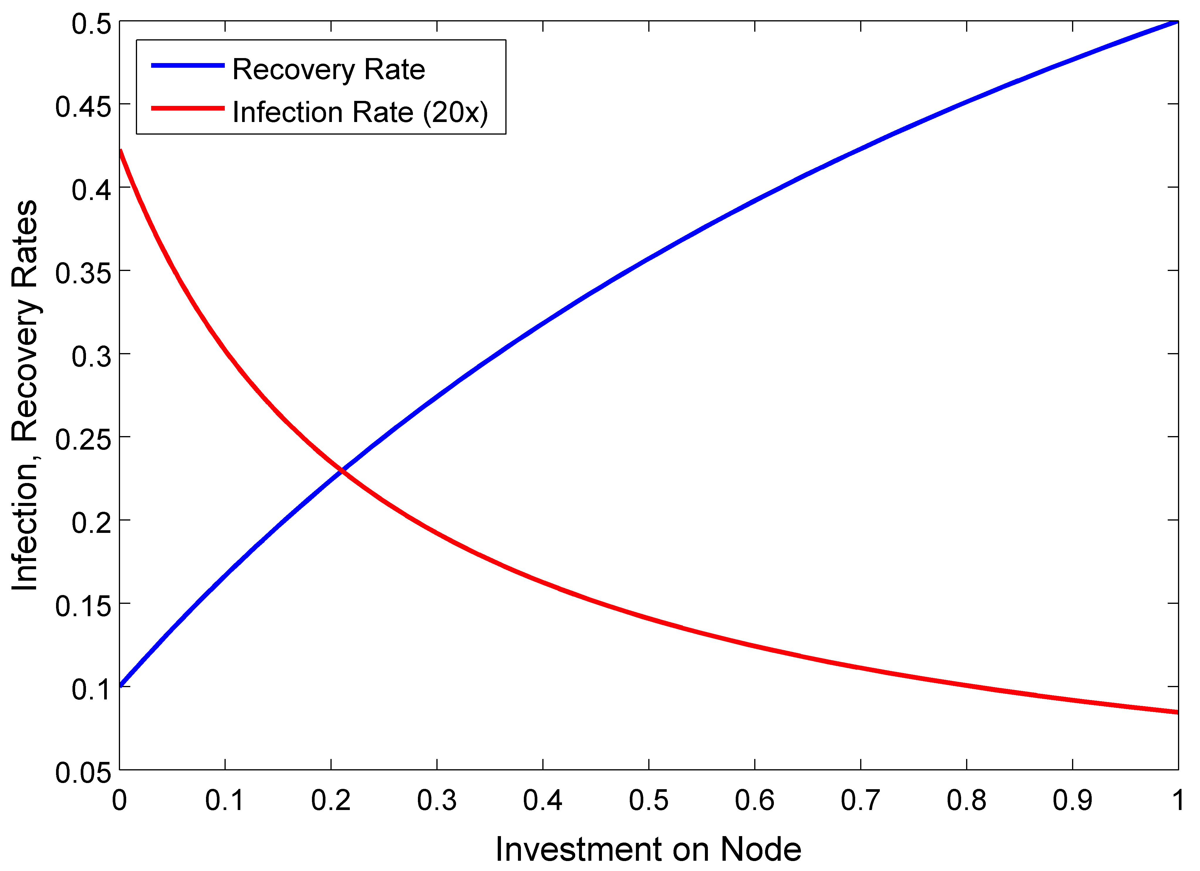
Figure 1: Infection rate (in red, and multiplied by 20, to improve visualization) and recovery rate (in blue) achieved at node $v_{i}$ after an investment on protection (in abscissas) is made on that node.

Using the air transformation network, the parameters, and the cost functions specified above, we solve both the rate-constrained and the budget-constrained allocation problem using the geometric programs in Theorems 11 and 12. The solution of the rate-constrained problem with $\overline{\varepsilon}=10^{-3}$ is summarized in Fig. 2. In the left subplot, we present a scatter plot with 56 circles (one circle per airport), where the abscissa of each circle is equal to $g_{i}\left(\delta_{i}^{*}\right)$ and the ordinate is $f_{i}\left(\beta_{i}^{*}\right)$, namely, the investments on correction and prevention on the airport at node $v_{i}$, respectively. We observe an interesting pattern in the allocation of preventive and corrective resources in the network. In particular, we have that in the optimal allocation some airports receive no resources at all (the circles associated to those airports are at the origin of the scatter plot); some airports receive only corrective resources (indicated by circles located on top of the $x$-axis), and some airports receive a mixture of preventive and corrective resources. In the center and right subplots in Fig. 2, we compare the distribution of resources with the in-degree and the PageRank centralities of the nodes in the network [23]. In the center subplot, we have a scatter plots where the ordinates represent investments on prevention (red +’s), correction (blue x’s), and total investment (the sum of prevention and correction investments, in black circles) for each airport, while the abscissas are the (weighted) in-degrees of the airports under consideration. We again observe a nontrivial pattern in the allocation of investments for protections. In particular, for airports with incoming traffic less than $5$ MPPY, no resources are invested at all, while for airports with incoming traffic between $5$ MPPY and $8$ MPPY, only corrective resources are needed. Airports with incoming traffic over $8$ MPPY receive both preventive and corrective resources. In the right subplot in Fig. 2, we include a scatter plot of the amount invested on prevention and correction for each airport versus its PageRank centrality in the transportation network. We observe that, although there is a strong correlation between centrality and investments, there is no trivial law to achieve the optimal resource allocation based on centrality measurements solely. For example, we observe in Fig. 2 how some airports receive a higher investment on protection than other airports with higher centrality. Hence, it is not always best for the most central nodes to receive the most resources. In [26], the authors expand on this phenomenon and propose digraphs in which resources allocated in the most central nodes have no effect on the exponential decay rate; these resources are effectively wasted.

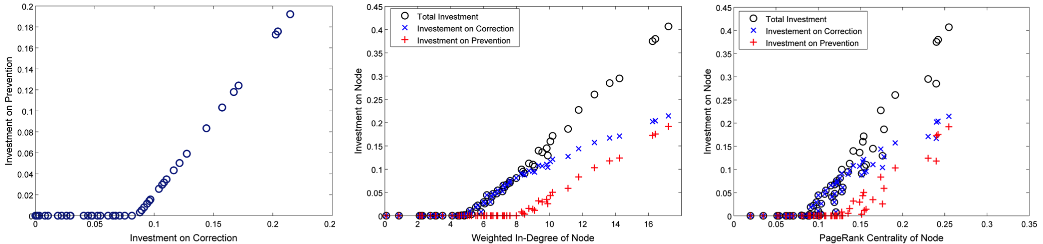
Figure 2: Results from the rate-constrained allocation problem. From left to right, we have (a) a scatter plot with the investment on correction versus prevention per node, (b) a scatter plot with the investment on protection per node and the in-degrees, and (c) a scatter plot with the investment on protection per node versus PageRank centralities.

Using Theorem 11, we also solve the budget-constrained allocation problem. We have chosen a budget that is a 50% extra over the optimal budget computed from Problem 2 with $\overline{\varepsilon}=10^{-3}$. With this extra budget, we achieve an exponential decay rate of $\varepsilon^{*}=0.342$. The corresponding allocation of resources is summarized in Fig. 3. The subplots in this figure are similar to those in Fig. 2, and we only remark the main differences in here. Notice that, given the extra budget, there are no airports with no investment on protection resources (as indicated by the absence of circles at the origin of the left subplot). Also, the center subplot indicates that all the airports receive a certain amount of corrective resources, although not all of them receive preventive resources (such as those with a (weighted) in-degree less than 4 MPPY). The scatter plot at the right illustrates the relationship between investments and PageRank centrality.

Figure 3: Results from the budget-constrained allocation problem. From left to right, we have (a) a scatter plot with the investment on correction versus prevention per node, (b) a scatter plot with the investment on protection per node and the in-degrees, and (c) a scatter plot with the investment on protection per node versus PageRank centralities.

V Conclusions

We have studied the problem of allocating protection resources in weighted, directed networks to contain spreading processes, such as the propagation of viruses in computer networks, cascading failures in complex technological networks, or the spreading of an epidemic in a human population. We have considered two types of protection resources: (i) Preventive resources able to ‘immunize’ nodes against the spreading (e.g. vaccines), and (ii) corrective resources able to neutralize the spreading after it has reached a node (e.g. antidotes). We assume that protection resources have an associated cost and have then studied two optimization problems: (a) The budget-constrained allocation problem, in which we find the optimal allocation of resources to contain the spreading given a fixed budget, and (b) the rate-constrained allocation problem, in which we find the cost-optimal allocation of protection resources to achieve a desired decay rate in the number of ‘infected’ nodes.

We have solved these optimal resource allocation problem in weighted and directed networks of nonidentical agents in polynomial time using Geometric Programming (GP). Furthermore, the framework herein proposed allows simultaneous optimization over both preventive and corrective resources, even in the case of cost functions being node-dependent.

We have illustrated our approach by designing an optimal protection strategy for a real air transportation network. We have limited our study to the network of the world’s busiest airports by passenger traffic. For this transportation network, we have computed the optimal distribution of protecting resources to contain the spread of a hypothetical world-wide pandemic. Our simulations show that the optimal distribution of protecting resources follows nontrivial patterns that cannot, in general, be described using simple heuristics based on traditional network centrality measures.

Proof of Lemma 9. We define the auxiliary matrix $M\triangleq\mbox{diag}\left(\beta_{i}\right)A-\mbox{diag}\left(\delta_{i}\right)+\Delta I$, where $\Delta\triangleq\max\left\{\delta_{i}\right\}$. Thus, $\lambda_{1}\left(M\right)=\lambda_{1}\left(\mbox{diag}\left(\beta_{i}\right)A-\mbox{diag}\left(\delta_{i}\right)\right)+\Delta$. Notice that both $M$ and $M^{T}$ are nonnegative and irreducible if $\mathcal{G}$ is strongly connected. Hence, from Lemma 6, there are two positive vectors $\mathbf{v}$ and $\mathbf{w}$ such that

$$M\mathbf{v} =\rho\mathbf{v},$$

$$\mathbf{w}^{T}M =\rho\mathbf{w}^{T},$$

where $\rho=\rho\left(M\right)=\lambda_{1}\left(M\right)$, and $\mathbf{v}$, $\mathbf{w}$ are the right and left dominant eigenvectors of $M$. From eigenvalue perturbation theory, we have that the increment in the spectral radius of $M$ induced by a matrix increment $\Delta M$ is [22]

$$\rho\left(M+\Delta M\right)-\rho\left(M\right)=\mathbf{w}^{T}\Delta M\mathbf{v}+o\left(\left\|\Delta M\right\|\right).$$ (45)

To study the effect of a positive increment in $\beta_{k}$ in the spectral radius, we define $\Delta B=\Delta\beta_{k}\mathbf{e}_{k}\mathbf{e}_{k}^{T}$, for $\Delta\beta_{k}>0$, and apply 45 with $\Delta M=\Delta B\,A$. Hence,

$$\rho\left(M+\Delta M\right)-\rho\left(M\right) =\Delta\beta_{k}\mathbf{w}^{T}\mathbf{e}_{k}\mathbf{e}_{k}^{T}A\mathbf{v}+o\left(\left\|\Delta\beta_{k}\right\|\right)$$

$$=\Delta\beta_{k}w_{k}\mathbf{a}_{k}^{T}\mathbf{v}+o\left(\left\|\Delta\beta_{k}\right\|\right)>0,$$

where $\mathbf{a}_{k}^{T}=\mathbf{e}_{k}^{T}A$ and the last inequality if a consequence of $\Delta\beta_{k}$, $w_{k}$, and $\mathbf{a}_{k}^{T}\mathbf{v}$ being all positive. Hence, a positive increment in $\beta_{k}$ induces a positive increment in the spectral radius.

Similarly, to study the effect of a positive increment in $\delta_{k}$ in the spectral radius, we define $\Delta D=\Delta\delta_{k}\mathbf{e}_{k}\mathbf{e}_{k}^{T}$, for $\Delta\delta_{k}>0$. Applying 45 with $\Delta M=-\Delta D$, we obtain

$$\rho\left(M+\Delta D\right)-\rho\left(M\right) =-\Delta\delta_{k}\mathbf{w}^{T}\mathbf{e}_{k}\mathbf{e}_{k}^{T}\mathbf{v}+o\left(\left\|\Delta\delta_{k}\right\|\right)$$

$$=-\Delta\delta_{k}w_{k}v_{k}+o\left(\left\|\Delta\delta_{k}\right\|\right)<0.$$

$\blacksquare$

Proof of Lemma 15. The proof of (a) is trivial and valid for any square matrix $M$. To prove (b), we consider the eigenvalue equations for $M$ and $RM$, i.e., $M\mathbf{u}=\lambda_{1}\left(M\right)\mathbf{u}$ and $RM\mathbf{w}=\lambda\mathbf{w}$, where $\mathbf{u}=\mathbf{v}_{1}\left(M\right)=\left[u_{i}\right]$ and $\mathbf{w}=\mathbf{v}_{1}\left(RM\right)=\left[w_{i}\right]$. We expand the eigenvalue equations component-wise as,

$$\sum_{j=1}^{n}m_{ij}u_{j} =\lambda u_{i},$$ (46)

$$\sum_{j=1}^{n}r_{i}m_{ij}w_{j} =\lambda w_{i},$$ (47)

for all $i=1,\ldots,n$. We now prove statement (b) by proving that $v_{i}=0$ if and only if $w_{i}=0$.

If $u_{i}=0$, then (46) gives $\sum_{j}m_{ij}v_{j}=0$. Since $m_{ij},v_{i}\geq 0$, the summation $\sum_{j}m_{ij}v_{j}=0$ if and only if the following two statements hold: (a1) $m_{ij}>0\implies v_{j}=0$ and (a2) $v_{j}>0\implies m_{ij}=0$. Since $t_{i}>0$, these two statements are equivalent to: (b1) $t_{i}m_{ij}>0\implies v_{j}=0$ and (b2) $v_{j}>0\implies t_{i}m_{ij}=0$. Statements (b1) and (b2) are true if and only if $\sum_{j}\left(t_{i}m_{ij}\right)w_{j}=0=w_{i}$, where the last equality comes from (47). Hence, we have that $v_{i}=0\iff w_{i}=0$; hence, $\mathcal{Z}\left(\mathbf{u}\right)=\mathcal{Z}\left(\mathbf{w}\right)$.

$\blacksquare$

Proof of Proposition 16. Our proof is based on the transformations defined in Lemma 15. Starting from a matrix $BA-D$, we then apply the following chain of transformations:

(i)

$T_{\alpha}\left(BA-D\right)=BA+\Delta$, for $\alpha=\max\left\{d_{i}\right\}$. Hence, $\Delta=\max\left\{d_{i}\right\}I-D$ and $BA+\Delta\geq 0$.

(ii)

$T_{R}\left(BA+\Delta\right)=\Delta^{-1}BA+I$, for $R=\Delta^{-1}$.

(iii)

$T_{\alpha}\left(\Delta^{-1}BA+I\right)=\Delta^{-1}BA$, for $\alpha=-1$.

(iv)

$T_{R}\left(\Delta^{-1}BA\right)=A$, for $R=B^{-1}\Delta$.

From Lemma 15, these transformations preserve the location of the zeros in the dominant eigenvector. Thus, the input to the first transformation, $BA-D$, and the output to the last transformation, $A$, satisfy $\mathcal{Z}\left(\mathbf{v}_{1}\left(BA-D\right)\right)=\mathcal{Z}\left(\mathbf{v}_{1}\left(A\right)\right)$.

$\blacksquare$

References

- [1] N. Bailey, The mathematical theory of infectious diseases and its applications. Charles Griffin & Company Ltd., 1975.
- [2] M. Garetto, W. Gong, and D. Towsley, “Modeling malware spreading dynamics,” in IEEE INFOCOM 2003, vol. 3, pp. 1869–1879, 2003.
- [3] S. Roy, M. Xue, and S. Das, “Security and discoverability of spread dynamics in cyber-physical networks,” IEEE Transactions on Parallel and Distributed Systems, vol. 23, no. 9, pp. 1694–1707, 2012.
- [4] Y. Wang, D. Chakrabarti, C. Wang, and C. Faloutsos, “Epidemic spreading in real networks: An eigenvalue viewpoint,” in Proc. 22nd Int. Symp. Reliable Distributed Systems, pp. 25–34, 2003.
- [5] A. Ganesh, L. Massoulie, and D. Towsley, “The effect of network topology on the spread of epidemics,” in IEEE INFOCOM 2005, vol. 2, pp. 1455–1466, 2005.
- [6] P. Van Mieghem, J. Omic, and R. Kooij, “Virus spread in networks,” IEEE/ACM Transactions on Networking, vol. 17, no. 1, pp. 1–14, 2009.
- [7] R. Cohen, S. Havlin, and D. Ben-Avraham, “Efficient immunization strategies for computer networks and populations,” Physical Review Letters, vol. 91, no. 24, p. 247901, 2003.
- [8] C. Borgs, J. Chayes, A. Ganesh, and A. Saberi, “How to distribute antidote to control epidemics,” Random Structures & Algorithms, vol. 37, no. 2, pp. 204–222, 2010.
- [9] F. Chung, P. Horn, and A. Tsiatas, “Distributing antidote using pagerank vectors,” Internet Mathematics, vol. 6, no. 2, pp. 237–254, 2009.
- [10] Y. Wan, S. Roy, and A. Saberi, “Designing spatially heterogeneous strategies for control of virus spread,” IET Systems Biology, vol. 2, no. 4, pp. 184–201, 2008.
- [11] E. Gourdin, J. Omic, and P. Van Mieghem, “Optimization of network protection against virus spread,” in 8th International Workshop on the Design of Reliable Communication Networks, pp. 86–93, 2011.
- [12] V. Preciado, F. Darabi Sahneh, and C. Scoglio, “A convex framework for optimal investment on disease awareness in social networks,” in IEEE Global Conference on Signal and Information Processing, pp. 851–854, 2013.
- [13] V. Preciado and M. Zargham, “Traffic optimization to control epidemic outbreaks in metapopulation models,” in IEEE Global Conference on Signal and Information Processing, pp. 847–850, 2013.
- [14] V. Preciado, M. Zargham, C. Enyioha, A. Jadbabaie, and G. Pappas, “Optimal vaccine allocation to control epidemic outbreaks in arbitrary networks,” in IEEE Conference on Decision and Control, 2013.
- [15] G. Weiss and M. Dishon, “On the asymptotic behavior of the stochastic and deterministic models of an epidemic,” Mathematical Biosciences, vol. 11, no. 3, pp. 261–265, 1971.
- [16] P. Van Mieghem and J. Omic, “In-homogeneous virus spread in networks,” arXiv preprint arXiv:1306.2588, 2013.
- [17] A. Barrat, M. Barthelemy, and A. Vespignani, Dynamical processes on complex networks. Cambridge University Press Cambridge, 2008.
- [18] J. Gleeson, S. Melnik, J. Ward, M. Porter, and P. Mucha, “Accuracy of mean-field theory for dynamics on real-world networks,” Physical Review E, vol. 85, p. 026106, 2012.
- [19] P. Van Mieghem, Performance analysis of communications networks and systems. Cambridge University Press, 2006.
- [20] S. Boyd and L. Vandenberghe, Convex optimization. Cambridge university press, 2004.
- [21] S. Boyd, S.-J. Kim, L. Vandenberghe, and A. Hassibi, “A tutorial on geometric programming,” Optimization and engineering, vol. 8, no. 1, pp. 67–127, 2007.
- [22] C. Meyer, Matrix analysis and applied linear algebra. SIAM, 2000.
- [23] M. Newman, Networks: An introduction. Cambridge University Press, 2010.
- [24] C. Schneider, T. Mihaljev, S. Havlin, and H. Herrmann, “Suppressing epidemics with a limited amount of immunization units,” Physical Review E, vol. 84, no. 6, p. 061911, 2011.
- [25] E. Nikolaidis, D. Ghiocel, and S. Singhal, Engineering Design Reliability Applications: For the Aerospace, Automotive and Ship Industries. CRC Press, 2007.
- [26] M. Zargham and V. Preciado, “Worst-case scenarios for greedy, centrality-based network protection strategies,” in ArXiv:1401.5753v1, 2014.