Two loop soft function for secondary massive quarks

Abstract

We present the calculation of the $\mathcal{O}(\alpha_{s}^{2}C_{F}T_{F})$ massive quark corrections to the soft function for the double hemisphere jet mass distribution in $e^{+}e^{-}$ collisions, a necessary ingredient for the calculation of several event shape distributions at N³LL order. The use of the mass as an infrared regulator allows us to derive the momentum space results for the massless quark structures at $\mathcal{O}(\alpha_{s}^{2}C_{F}T_{F}n_{f})$ and the gluonic structures at $\mathcal{O}(\alpha_{s}^{2}C_{A}C_{F})$, which have not been given so far in the literature. Furthermore, we compute the corresponding corrections in the soft function for thrust, the most prominent projection of the double hemisphere mass distribution. Finally we give expressions for the corresponding renormalon subtractions in the gap scheme.

I Introduction

The theoretical description of event shape distributions in $e^{+}e^{-}$ collisions has recently seen substantial progress concerning the treatment of higher-order QCD corrections Weinzierl:2008iv ; Weinzierl:2009ms ; GehrmannDeRidder:2007bj ; GehrmannDeRidder:2007hr , the techniques concerning the summation of large logarithmic terms Becher:2008cf ; Chien:2010kc ; Becher:2012qc ; Chiu:2011qc ; Chiu:2012ir ; Gehrmann:2012sc and the implementation of schemes that avoid renormalon ambiguities together with the definition of non-perturbative parameters Hoang:2007vb ; Hoang:2009yr . These developments have contributed to an improved theoretical accuracy for the description of event shape distributions and to precise measurements of QCD parameters such as the strong coupling Abbate:2010xh ; Abbate:2012jh ; Gehrmann:2009eh ; Gehrmann:2012sc . An important development for making higher order corrections accessible in a systematic way is the framework of Soft-Collinear Effective Theory (SCET) Bauer:2000ew ; Bauer:2000yr which makes it possible to factorize the most singular contributions for a large class of event shapes in the dijet limit in terms of a hard current Wilson coefficient, a jet function describing the collinear radiation and a soft function describing large-angle soft radiation. Within the SCET framework it has also become possible to treat coherently the effects of the production of massive quarks which are the focus of this work. In $e^{+}e^{-}$-collisions one can distinguish two types of heavy quark production mechanisms: primary, where the heavy quarks are produced directly by the hard current, and secondary, where massless quarks are produced by the hard current and the heavy quarks arise from gluon splitting.

For the production of primary heavy quarks, factorization in the dijet limit for the c.m. energy being much larger than the mass was discussed in Ref. Fleming:2007qr and results suitable for a description at NNLL order Fleming:2007xt were provided for the case that the quark mass is of order of the jet invariant mass. An important conceptual finding of Ref. Fleming:2007xt was that, as long as only secondary radiation of massless partons is considered, the soft function remains unchanged with respect to the case of primary massless quark production in the dijet limit, so that only the jet function receives non-trivial modifications due to the heavy quark mass. It was further shown for the same situation that approaching the heavy quark production threshold in the collinear sector when the off-shellness is much smaller than the heavy quark mass, an additional matching onto boosted versions of Heavy-Quark Effective Theory (HQET) is required, which does not affect the soft sector.

For the production of secondary heavy quarks no coherent approach of how the quark mass affects factorization has been presented until recently. While it was known that at LL and NLL order the main effect is related to the number of active running quark flavors in the evolution equations for the strong coupling and the renormalization group factors in the factorization theorem Fleming:2007qr ; Kaplan:2008pt , the conceptual background of how to go beyond NLL order, which includes non-trivial matrix element corrections and matching conditions was only provided recently in Ref. Gritschacher:2013pha . In that work it was shown that the problem of secondary heavy quark production is closely related to the problem of massive gauge boson production in jet observables, because the production of a heavy quark-antiquark pair off a virtual gluon can be calculated from a dispersion integral over the gluon invariant mass. In addition to the usual collinear and soft degrees of freedom known for the purely massless case, the resulting factorization framework requires so-called mass modes, which are collinear and soft degrees of freedom with a common typical invariant mass of the order of the heavy quark mass. The mass modes are integrated out when the evolution crosses the heavy quark mass threshold and allow for a continuous description of the singular terms from infinitely heavy down to infinitesimally small masses merging into the known massless limit. It was also demonstrated in Ref. Gritschacher:2013pha that when the mass modes are integrated out the associated matching conditions in the collinear and soft sectors can involve non-trivial plus-distributions in the respective kinematic variables.

The above mentioned dispersion method is exact for cases where the momenta of the produced massive quark and antiquark momenta enter the observable in a coherent manner such as for the calculation of the jet function or for purely virtual corrections like the ones entering the hard current Wilson coefficient. On the other hand, for the soft function, where the two quarks can enter into different hemispheres and their momenta contribute incoherently due to phase space constraints, the dispersion method does not lead to the correct finite non-logarithmic corrections. Thus the ${\cal O}(\alpha_{s}^{2}C_{F}T_{F})$ massive quark corrections to the soft function have to be determined by a dedicated computation along the lines of Ref. Kelley:2011ng where the ${\cal O}(\alpha_{s}^{2})$ corrections to the soft function from gluons and massless quarks were determined by lengthy calculations (see also Ref. Hornig:2011iu for a discussion of non-global logarithms at ${\cal O}(\alpha_{s}^{2})$ as well as Hoang:2008fs ). It is the main aim of this paper to present and discuss the ${\cal O}(\alpha_{s}^{2}C_{F}T_{F})$ massive quark corrections to the double hemisphere soft function and to outline their calculation. The results are important for event shapes such as thrust and the heavy jet mass. We assume for the most part of this paper that the heavy quark mass is of the order of the typical soft momenta, so we consider virtual as well as real corrections due to secondary massive quark production accounting for the exact analytic threshold behavior.

An interesting conceptual feature of the result is that the quark mass serves as a physical infrared regulator which provides a manifest separation of IR-sensitive and UV-divergent structures. This separation is less obvious and more difficult to make manifest for the massless case when IR and UV divergences are regularized by dimensional regularization. Using the ${\cal O}(\alpha_{s}^{2}C_{F}T_{F})$ massive quark corrections to the soft function and the fact that the UV-divergences agree with the massless quark case, it is possible to determine the distributive analytical structure of the ${\cal O}(\alpha_{s}^{2}C_{F}T_{F}n_{f})$ massless quark corrections to the momentum space double hemisphere soft function. Taking these steps as a guideline one can then also deduce the momentum space representation for all ${\cal O}(\alpha_{s}^{2})$ corrections. This analytical distributive structure of the momentum space double hemisphere soft function was not identified in Refs. Kelley:2011ng ; Hornig:2011iu and represents an additional result of this work.

The finite quark mass also provides a physical cutoff against infrared renormalons that arise for massless quarks in high order corrections and enhance the sensitivity to small gluon virtuality. In this work we nevertheless discuss the subtraction of the perturbative ${\cal O}(\Lambda_{\rm QCD})$ renormalon contributions along the lines of Refs. Hoang:2007vb ; Jain:2008gb ; Hoang:2008fs for the $\mathcal{O}(\alpha_{s}C_{F}T_{F})$ massive quark corrections. The knowledge of this subtraction is required in cases when the quark mass decreases below the scale of the soft radiation in order to achieve a continuous transition to the massless approximation which has been used in many previous analyses. It is also required for the determination of the matching condition when the R-evolution in the renormalon-subtracted scheme Hoang:2008yj ; Hoang:2009yr for the soft power correction Hoang:2007vb ; Jain:2008gb ; Hoang:2008fs crosses the mass threshold.

The content of this paper is as follows: In Sec. II we summarize briefly the SCET factorization theorem for double hemisphere masses in the dijet region. Since the computation of the soft hemisphere function involves several steps we first give an outline of the method we use in Sec. III followed by the explicit details of the corresponding phase space calculations given in Secs. IV and V. In Sec. VI we use our results with massive quarks to derive explicit expressions for the massless limit of the soft hemisphere function. As an explicit example for an event shape derived from the hemisphere masses we discuss the massive thrust soft function in Sec. VII. In Sec. VIII we present the results for the corresponding renormalon subtractions of the massive soft function, before we conclude in Sec. IX.

II Factorization Theorem and Soft Function Definition

We focus on the dijet invariant mass distribution in $e^{+}e^{-}$ annihilation, where one defines two hemispheres (left/right) separated by the plane perpendicular to the thrust axis $\mathbf{n}$. The factorization theorem for the singular terms in the dijet limit, where the c.m.energy $Q$ is much larger than the jet masses, accounting only for massless secondary quarks has the form Fleming:2007qr ; Fleming:2007xt

$$\frac{1}{\sigma_{0}}\frac{d^{2}\sigma}{dM_{l}^{2}dM_{r}^{2}}= \,H(Q,\mu^{2})\int dk_{l}\,dk_{r}\,J_{n}(M_{l}^{2}-Qk_{l},\mu)$$

$$\times\,J_{\bar{n}}(M_{r}^{2}-Qk_{r},\mu)\,S(k_{l},k_{r},\mu)\,,$$ (1)

where the hemisphere mass $M_{l}$ ($M_{r}$) denotes the invariant mass in the left (right) hemisphere. The terms $H(Q,\mu)$, $J_{n,\bar{n}}(s,\mu)$, $S(k_{l},k_{r},\mu)$ are the hard, jet and soft functions and all renormalization group factors which sum large logarithms are implicit. The knowledge of the double differential distribution allows us to derive the differential cross sections for several other event shape variables like thrust via

$$\frac{d\sigma}{d\tau}=\int dM_{l}^{2}dM_{r}^{2}\,\frac{d^{2}\sigma}{dM_{l}^{2}dM_{r}^{2}}\,\delta\left(\tau-\frac{M_{l}^{2}}{Q^{2}}-\frac{M_{r}^{2}}{Q^{2}}\right)$$ (2)

in the dijet limit.

In the case of massive secondary particles the basic structure of the factorization theorem in Eq. (II) remains unchanged when the quark mass is close to the soft scale $\mu_{S}\sim k_{l}\sim k_{r}\sim Q\tau$ Gritschacher:2013pha . In this case the massive quarks contribute in a nontrivial way only to the singular terms in the soft function $S$. So for the purpose of this work we for the most part consider $n_{f}$ massless quark flavors and one additional quark flavor with mass $m\sim\mu_{S}\sim Q\tau\ll Q$ in the dijet limit. The hemisphere soft function in the factorization theorem in Eq. (II) is defined as

$$S(k_{r},k_{l},m,\mu)\equiv \,\frac{1}{N_{c}}\sum_{X_{s}}\,\langle 0\lvert\overline{Y}_{\bar{n}}Y_{n}(0)\lvert X_{s}\rangle\langle X_{s}\lvert Y_{n}^{\dagger}\overline{Y}_{\bar{n}}^{\dagger}(0)\lvert 0\rangle$$

$$\times\delta(k_{l}-\bar{n}\cdot k_{s}^{l})\,\delta(k_{r}-n\cdot k_{s}^{r})\,,$$ (3)

where $k_{s}^{l}$ ($k_{s}^{r}$) is the light-cone momentum of the soft final state $\lvert X_{s}\rangle$ in the left (right) hemisphere and $Y_{n}(x)$, $\overline{Y}_{\bar{n}}(x)$ are ultrasoft Wilson lines, i.e.

$$Y_{n}(x) \equiv\overline{\textrm{P}}\,\textrm{exp}\left[-ig\int_{0}^{\infty}ds\,n\cdot A_{us}(ns+x)\right]\,,$$

$$\overline{Y}_{\bar{n}}(x) \equiv\overline{\textrm{P}}\,\textrm{exp}\left[-ig\int_{0}^{\infty}ds\,\bar{n}\cdot\overline{A}_{us}(ns+x)\right]$$ (4)

with $\bar{A}_{\mu}=\bar{T}^{A}A_{\mu}^{A}$ and $\bar{T}^{A}=-(T^{A})^{T}$. We have indicated the dependence of the soft function on the quark mass by the additional argument $m$. For purely massless quarks the ${\cal O}(\alpha_{s}^{2})$ corrections to the partonic hemisphere soft function have been computed in Ref. Kelley:2011ng , see also Ref. Hornig:2011iu . In the following, we will calculate the ${\cal O}(\alpha_{s}^{2}C_{F}T_{F})$ corrections from massive quarks due to gluon splitting as shown in the diagrams of Fig. 1. The generalization to several massive quark flavors is straightforward. We emphasize that the definition of the soft function in Eq. (3) also applies for the case when the primary quarks are massive Fleming:2007qr ; Fleming:2007xt as long as the c.m. energy $Q$ is much larger than their mass since the emergence of the Wilson lines in the soft Eikonal approximation is mass-independent. So our result also applies for massive secondary quark effects in massive primary quark production, where masses of primary and secondary quarks can differ, up to potential trivial modifications concerning the scheme for $\alpha_{s}$.

III Outline of the calculation

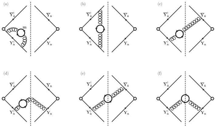
Figure 1: The types of Feynman diagrams for the $\mathcal{O}(\alpha_{s}^{2}C_{F}T_{F})$ contributions to the soft function with corresponding symmetric configurations. (a) and (b) are purely virtual, (c) and (d) contain the contributions to real gluon radiation and (e) and (f) the contributions for the real radiation of a quark-antiquark pair. (a) and (d) vanish due to $n\cdot n=0$.

We compute the diagrams in Fig. 1 for one quark flavor with mass $m$. While the phase space for the diagrams (a) - (d) is easy, the computation of diagrams (e) and (f) is non-trivial, when the massive quark and antiquark with momenta $k$ and $q$, respectively, enter the final state. Taking into account the corresponding symmetry factors, one can obtain their contributions to the soft function in the form analogously to the massless case Kelley:2011ng

$$S_{e+f}(k_{r},k_{l},m)= \int\frac{d^{d}k}{(2\pi)^{d}}\int\frac{d^{d}q}{(2\pi)^{d}}\,F^{(qq)}(k,q,k_{r},k_{l},m)$$

$$\times s(k,q)\,,$$ (5)

where $s(k,q)$ is the matrix element calculated by conventional Feynman rules,

$$s(k,q)=g^{4}C_{F}T_{F}\tilde{\mu}^{2\epsilon}\frac{4(k^{+}q^{-}+k^{-}q^{+}-2k\cdot q)}{(k^{+}+q^{+})(k^{-}+q^{-})(k+q)^{4}}\,.$$ (6)

The phase space constraints and the on-shell condition for the massive quarks are given by the quark hemisphere prescription $F^{(qq)}(k,q,k_{r},k_{l},m)$,

$$F^{(qq)}(k,q,k_{r},k_{l},m)=$$

$$(-2\pi i)^{2}\,\delta(k^{2}-m^{2})\,\delta(q^{2}-m^{2})\,\theta(k^{+}+k^{-})\,\theta(q^{+}+q^{-})$$

$$\times\left[\theta(k^{+}-k^{-})\,\theta(q^{-}-q^{+})\,\delta(q^{+}-k_{r})\,\delta(k^{-}-k_{l})\right.$$

$$\hskip 5.69046pt+\theta(k^{-}-k^{+})\,\theta(q^{+}-q^{-})\,\delta(k^{+}-k_{r})\,\delta(q^{-}-k_{l})$$

$$\hskip 5.69046pt+\theta(k^{-}-k^{+})\,\theta(q^{-}-q^{+})\,\delta(k^{+}+q^{+}-k_{r})\,\delta(k_{l})$$

$$\hskip 5.69046pt+\left.\theta(k^{+}-k^{-})\,\theta(q^{+}-q^{-})\,\delta(k^{-}+q^{-}-k_{l})\,\delta(k_{r})\right]\,.$$ (7)

Solving the integral (III) directly with this phase space constraint turns out to be an extraordinarily difficult task due to the mass dependence together with the complications that arise from the parts of the phase space where the quark and antiquark enter different hemispheres. Instead of approaching with brute force, we therefore apply the following strategy: We first calculate a soft function with a much simpler phase space constraint (but the same matrix element),

$$S_{e+f}^{(g)}(k_{r},k_{l},m)= \int\frac{d^{d}k}{(2\pi)^{d}}\int\frac{d^{d}q}{(2\pi)^{d}}\,F^{(g)}(k,q,k_{r},k_{l},m)$$

$$\times s(k,q)\,,$$ (8)

where the phase space constraints are given by the gluon hemisphere prescription $F^{(g)}(k,q,k_{r},k_{l},m)$,

$$F^{(g)}(k,q,k_{r},k_{l},m)=$$

$$(-2\pi i)^{2}\,\delta(k^{2}-m^{2})\,\delta(q^{2}-m^{2})\,\theta(k^{+}+k^{-})\,\theta(q^{+}+q^{-})$$

$$\times\left[\theta(k^{+}+q^{+}-k^{-}-q^{-})\,\delta(k_{r})\,\delta(k^{-}+q^{-}-k_{l})\right.$$

$$\hskip 5.69046pt+\left.\theta(k^{-}+q^{-}-k^{+}-q^{+})\,\delta(k_{l})\,\delta(k^{+}+q^{+}-k_{r})\right]\,.$$ (9)

This phase space assigns the soft hemisphere momenta coherently to the components of the gluon momentum $k+q$, so that the massive quark and antiquark momenta always contribute together and homogeneously to $k_{l}$ and $k_{r}$. The soft function obtained in this way only keeps track of the hemisphere, into which the virtual gluon propagated, and therefore differs from the actual physical hemisphere soft function we aim to calculate, where the final state partons each are accounted for in the hemisphere they propagate. Since both prescriptions are compatible with soft-collinear factorization and lead to the same hard current and jet functions, the consistency of the renormalization group evolution forces both soft functions to have the same UV divergences. So the required additional correction arising from the difference between the quark hemisphere and gluon hemisphere prescription, which we call phase space misalignment correction, can be computed in four dimensions, which can be tackled numerically. Due to the finite quark masses the resulting calculations are also IR-finite and straightforward to carry out.

The advantage of introducing the gluon hemisphere prescription is that the kinematics is only governed by the gluon momenta weighted by the gluon virtuality. So in the calculation the physical effects associated to the fact that a massive quark pair is produced from virtual gluon decay can be separated from the computation of the phase space. This makes the gluon hemisphere prescription quite simple to compute because it allows us to perform the computation with the help of dispersion integrations over the gluon virtuality as described in Refs. Kniehl:1988id ; Hoang:1994it ; Hoang:1995ex : As a first step one calculates the ${\cal O}(\alpha_{s})$ corrections to the partonic soft function coming from the radiation of a “massive gluon” with momentum $p=k+q$. Then, by convoluting the massive gluon result with the imaginary part of the gluon vacuum polarization function related to the massive quark cuts in diagrams (e) and (f) one obtains the ${\cal O}(\alpha_{s}^{2}C_{F}T_{F})$ massive quark corrections in the gluon hemisphere prescription. The calculation is very generic and it is trivial to determine the effects of gluon splitting into any other kind of final state, such as gluino pairs, just to mention one example. Note that the method applies regardless of whether the physical effects are related to virtual corrections or real radiation final states.

To explain the dispersion method for an equal-mass quark-antiquark pair we start with the gluonic vacuum polarization $\Pi(m^{2},p^{2})$ contribution arising from a massive quark-antiquark bubble,

$$-i\left(p^{2}g_{\mu\nu}-p_{\mu}p_{\nu}\right)\Pi(m^{2},p^{2})\,\delta^{AB}$$

$$\equiv\int d^{4}x\,e^{ipx}\,\langle 0\lvert T\left[J_{\mu}^{A}(x)J_{\nu}^{B}(0)\right]\lvert 0\rangle\,,$$ (10)

with the current $J^{A}_{\mu}(x)=ig_{s}\bar{q}(x)T^{A}\gamma_{\mu}q(x)$, which can be expressed through an integral over its absorptive part. The unsubtracted (unrenormalized) dispersion integral reads

$$\Pi(m^{2},p^{2})=-\frac{1}{\pi}\int{dM^{2}\,\frac{\mathrm{Im}\left[\Pi(m^{2},M^{2})\right]}{p^{2}-M^{2}+i\epsilon}}\,,$$ (11)

where the absorptive part in $d$ dimensions reads

$$\mathrm{Im}\left[\Pi(m^{2},p^{2})\right]=\theta(p^{2}-4m^{2})\,g^{2}T_{F}\tilde{\mu}^{2\epsilon}(p^{2})^{(d-4)/2}$$

$$\times\frac{2^{3-2d}\pi^{(3-d)/2}}{\Gamma\left(\frac{d+1}{2}\right)}\left(d-2+\frac{4m^{2}}{p^{2}}\right)\left(1-\frac{4m^{2}}{p^{2}}\right)^{(d-3)/2}\,.$$ (12)

We call this dispersion relation “unrenormalized” because it is related to the calculation where the strong coupling is still unrenormalized (with respect to the effects of the massive quark flavor). At this point the standard scheme choices for the renormalization of the strong coupling are the $\overline{\rm MS}$ scheme involving the subtraction of the $1/\epsilon$ divergence in $\Pi(m^{2},p^{2})$ or the on-shell subtraction scheme involving the subtraction of $\Pi(m^{2},p^{2}=0)$. Using the $\overline{\rm MS}$ scheme means that the massive quark is active concerning the renormalization group evolution, so the strong coupling evolves with $n_{f}+1$ active dynamical flavors. Using on-shell subtractions means that that the massive quark is not active concerning the renormalization group, so the strong coupling evolves with $n_{f}$ active dynamical flavors. The on-shell subtraction is used when the massive quark is integrated out and can also be implemented into the dispersion relation itself by employing its subtracted form

$$\Pi^{\rm OS}(m^{2},p^{2}) =\Pi(m^{2},p^{2})-\Pi(m^{2},0)$$

$$=-\frac{p^{2}}{\pi}\int{\frac{dM^{2}}{M^{2}}\,\frac{\mathrm{Im}\left[\Pi(m^{2},M^{2})\right]}{p^{2}-M^{2}+i\epsilon}}\,.$$ (13)

The subtracted dispersion relation has an important computational advantage since the integration over the virtual gluon mass is suppressed by an additional power of $1/M^{2}$ for large values of $M^{2}$. This property can make the dispersion integration finite and may allow us to carry out the integral directly in $d=4$ dimensions. The unrenormalized result can then be easily recovered by adding back the massless gluon result times $\Pi(m^{2},p^{2}=0)$. We will use this method in the following.

To be definite, the correction to the Feynman gauge gluon propagator due to a massive quark-antiquark loop expressed in terms of the subtracted dispersion relation reads

$$\Pi_{\mu\nu}^{\textnormal{eff,OS}}(m^{2},p^{2})\equiv\,\frac{(-i)^{2}g_{\mu\rho}\Pi^{\rho\sigma,{\rm OS}}(m^{2},p^{2})\,g_{\sigma\nu}}{(p^{2}+i\epsilon)^{2}}$$

$$=\,\frac{1}{\pi}\int\frac{dM^{2}}{M^{2}}\,\frac{-i\left(g_{\mu\nu}-\frac{p_{\mu}p_{\nu}}{p^{2}}\right)}{p^{2}-M^{2}+i\epsilon}\,\mathrm{Im}\left[\Pi(m^{2},M^{2})\right]\,,$$ (14)

where $p^{\mu}$ denotes the external gluon momentum, and we have dropped from the equalities the overall color conserving Kronecker $\delta^{AB}$. Note that in Eq. (14) the propagator becomes transverse from the insertion of the vacuum polarization. In our calculations the contributions from the additional $p^{\mu}p^{\nu}$ term vanish due to gauge invariance and can be ignored. The relation also shows explicitly that we can obtain the result for the massive quark-antiquark pair from a dispersion integral over the corresponding result for a gluon with mass $M$. Thus we can obtain the ${\cal O}(\alpha_{s}^{2}C_{F}T_{F})$-corrections to the soft function in the gluon hemisphere prescription with the on-shell subtraction for the strong coupling by the relation

$$S_{\rm{OS}}^{(g)}(k_{l},k_{r},m,\mu)= \,\frac{1}{\pi}\int\frac{dM^{2}}{M^{2}}\,S^{(1)}_{M}(k_{l},k_{r},M,\mu)$$

$$\times\mathrm{Im}\left[\Pi(m^{2},M^{2})\right]\,,$$ (15)

where $S^{(1)}_{M}$ denotes the one-loop massive gluon contribution to the soft function. The corresponding result with the more common $\overline{\rm MS}$ subtraction then reads

$$S_{\rm{\overline{MS}}}^{(g)}(k_{l},k_{r},m,\mu)=S_{\rm{OS}}^{(g)}(k_{l},k_{r},m,\mu)$$

$$-\left(\Pi(m^{2},0)-\frac{\alpha_{s}T_{F}}{3\pi}\,\frac{1}{\epsilon}\right)\times S^{(1)}(k_{l},k_{r},\mu)\,$$ (16)

with $S^{(1)}$ being the massless one-loop contribution to the soft function. For convenience we also give the result for the zero-momentum vacuum polarization function in $d$ dimensions:

$$\Pi(m^{2},0)=\frac{\alpha_{s}T_{F}}{3\pi}\left(\frac{\mu^{2}}{m^{2}}\right)^{\epsilon}\Gamma(\epsilon)e^{\gamma_{E}\epsilon}\,.$$ (17)

IV Massive quark corrections with gluon hemisphere prescription

We start with the computation of ${\cal O}(\alpha_{s}^{2}C_{F}T_{F})$ massive quark corrections to the soft function with the gluon hemisphere prescription, $S^{(g)}(k_{r},k_{l},m,\mu)$, along the lines described above.

IV.0.1 Soft function for massive gluons at ${\cal O}(\alpha_{s})$

In the calculations for the ${\cal O}(\alpha_{s})$ soft function with a massive gluon, we encounter rapidity divergences in individual parts of the computation which are not regularized by dimensional regularization. Although the rapidity divergences cancel in the sum of all terms Gritschacher:2013pha , it is convenient to implement an additional regulator. In any case, using a regulator, all integrals are well defined individually, and the outcome for the different diagrams is regulator-dependent. We choose the “$\alpha$-regulator” Smirnov:1997gx ; Becher:2011dz

$$\int dp^{-}\rightarrow\int dp^{-}\left(\frac{\nu}{p^{-}}\right)^{\alpha}\,$$ (18)

on the minus gluon momentum component. We use the $\alpha$-regulator in a way more general than advocated in Ref. Becher:2011dz since we apply it not only for phase space integrations but also for loop diagrams, so that some of the properties of this regulator for phase space integrals as stated in Ref. Becher:2011dz might not hold. The exact implementation of the regularization of rapidity divergences is only of minor importance for our calculation since the divergences cancel entirely within the soft function computation and no large logarithms arise when the mass is of order of the soft scale. With the regulator (18) the purely virtual diagram in Fig. 1 (b) yields a scaleless integral and vanishes, so only the diagrams containing the real radiation of a massive gluon are non-vanishing.

The diagrams for real radiation of a gluon with mass $M$ in $d$-dimensions, after expanding in $\alpha$, yield ($\bar{k}=k/\mu$)

$$\mu^{2}S^{(1)}_{M}(k_{r},k_{l},M,\mu)=\frac{\alpha_{s}(\mu)C_{F}}{4\pi}\,\delta(\bar{k}_{l})\left\{\left(\frac{\mu^{2}}{M^{2}}\right)^{\epsilon}e^{\gamma_{E}\epsilon}\Gamma(\epsilon)\right.$$

$$\times\left(2\,\delta(\bar{k}_{r})\left[\textrm{ln}\left(\frac{\mu^{2}}{M^{2}}\right)+\gamma_{E}-\psi(\epsilon)\right]+4\left[\frac{\theta(\bar{k}_{r})}{\bar{k}_{r}}\right]_{+}\right)$$

$$\left.-\,\theta(k_{r}-M)\frac{4}{\bar{k}_{r}}\,\textrm{ln}\left(\frac{k_{r}^{2}}{M^{2}}\right)\right\}+(k_{r}\leftrightarrow k_{l})\,.$$ (19)

Note that the threshold term involving the $\theta$-function corresponds to real radiation. It has been given for $d=4$ ($\epsilon=0$) because it only involves IR and UV finite integrals within the subtracted dispersion integral (15). Technical details on the calculation leading to Eq. (IV.0.1) can be found in Gritschacher:2013pha .

IV.0.2 Massive quark corrections at ${\cal O}(\alpha_{s}^{2})$

We use the dispersive technique to obtain the ${\cal O}(\alpha_{s}^{2}C_{F}T_{F})$ part of the soft function for massive quarks. The convolution along the lines of Eq. (15) is performed separately for the $d$ dimensional virtual terms and the four-dimensional threshold term in Eq. (IV.0.1), where for the latter the $d=4$ version of the absorptive part of the vacuum polarization function in Eq. (III) can be used. We encounter hypergeometric functions, which are expanded with the $HypExp$ package Huber:2005yg in $Mathematica$. The structure of the result with on-shell subtraction for the strong coupling ($\alpha_{s}=\alpha_{s}^{(n_{f})}$) reads

$$S^{(g)}_{OS}(k_{l},k_{r},m,\mu)=S^{(g)}_{OS,\rm virt}(k_{l},k_{r},m,\mu)+S^{(g)}_{\rm real}(k_{l},k_{r},m)\,,$$ (20)

where the unrenormalized distributive part $S^{(g)}_{OS,\rm virt}$ describing virtual radiation reads

$$\mu^{2}S^{(g)}_{OS,\rm virt}(k_{l},k_{r},m,\mu)=\frac{\alpha_{s}^{2}C_{F}T_{F}}{16\pi^{2}}\,\delta(\bar{k}_{l})\bigg{\{}\delta(\bar{k}_{r})$$

$$\times\left[-\frac{2}{\epsilon^{3}}+\frac{1}{\epsilon^{2}}\left(\frac{8}{3}L_{m}+\frac{10}{9}\right)+\frac{1}{\epsilon}\left(-\frac{4}{3}L_{m}^{2}+\frac{56}{27}-\frac{\pi^{2}}{3}\right)\right.$$

$$-\left.\frac{20}{9}L_{m}^{2}+\left(-\frac{224}{27}+\frac{4\pi^{2}}{9}\right)L_{m}-\frac{328}{27}+\frac{5\pi^{2}}{27}+4\zeta(3)\right]$$

$$+\left[\frac{\theta(\bar{k}_{r})}{\bar{k}_{r}}\right]_{+}\left[\frac{8}{3\epsilon^{2}}+\frac{1}{\epsilon}\left(-\frac{16}{3}L_{m}-\frac{40}{9}\right)+\frac{16}{3}L_{m}^{2}+\frac{80}{9}L_{m}\right.$$

$$+\left.\left.\frac{224}{27}+\frac{4\pi^{2}}{9}\right]\right\}+(k_{r}\leftrightarrow k_{l})\,,$$ (21)

with $L_{m}=\textrm{ln}(m^{2}/\mu^{2})$. The finite threshold part $S^{(g)}_{\rm real}(k_{l},k_{r},m,\mu)$ describing real radiation and vanishing for $k_{l,r}\leq 2m$ reads

$$\mu^{2}S^{(g)}_{\rm real}(k_{l},k_{r},m)=\frac{\alpha_{s}^{2}C_{F}T_{F}}{16\pi^{2}}\,\delta(\bar{k}_{l})\,\theta(k_{r}-2m)$$

$$\times\frac{1}{\bar{k}_{r}}R\left(\sqrt{1-\frac{4m^{2}}{k_{r}^{2}}}\right)+(k_{r}\leftrightarrow k_{l})\,,$$ (22)

where the real radiation function is given by

$$R(w)=\frac{32}{3}\textrm{Li}_{2}\left(\frac{w-1}{w+1}\right)+\frac{16}{3}\textrm{ln}^{2}\left(\frac{1+w}{2}\right)$$

$$-\frac{16}{3}\textrm{ln}^{2}\left(\frac{1-w}{2}\right)+\frac{8}{3}\textrm{ln}^{2}\left(\frac{1+w}{1-w}\right)+\frac{80}{9}\textrm{ln}\left(\frac{1+w}{1-w}\right)$$

$$+\frac{32}{27}w^{3}-\frac{160}{9}w+\frac{8\pi^{2}}{9}\,.$$ (23)

To obtain the result with $\overline{\rm MS}$ subtraction for the strong coupling ($\alpha_{s}=\alpha_{s}^{(n_{f}+1)}$) one has to add the $\overline{\rm MS}$-renormalized finite contributions of the zero momentum vacuum polarization according to Eq. (16). This gives the additional contributions

$$\delta S^{(g)}(k_{r},k_{l},m,\mu)=-\left(\Pi(m^{2},0)-\frac{1}{\epsilon}\right)\times S^{(1)}(k_{r},k_{l},\mu)$$

$$=-\frac{\alpha_{s}T_{F}}{3\pi}\left[\left(\frac{\mu^{2}}{m^{2}}\right)^{\epsilon}\Gamma(\epsilon)e^{\gamma_{E}\epsilon}-\frac{1}{\epsilon}\right]\times\frac{\alpha_{s}C_{F}}{\pi}\frac{\mu^{2\epsilon}e^{\gamma_{E}\epsilon}}{\epsilon\Gamma(1-\epsilon)}$$

$$\hskip 11.38092pt\times\left[\delta(k_{l})\theta(k_{r})k_{r}^{-1-2\epsilon}+(k_{r}\leftrightarrow k_{l})\right]\,.$$ (24)

The contributions in Eq. (IV.0.2) contain only the virtual distributive pieces and do not affect the massive quark real radiation corrections. Expanded for small $\epsilon$ the unrenormalized ${\cal O}(\alpha_{s}^{2}C_{F}T_{F})$ massive quark contributions to the soft function (with $\overline{\rm MS}$ renormalized $\alpha_{s}^{(n_{f}+1)}$) read

$$S^{(g)}(k_{r},k_{l},m,\mu)= \,S^{(g)}_{OS}(k_{l},k_{r},m,\mu)+\delta S^{(g)}(k_{r},k_{l},m,\mu)$$

$$= \,Z_{S,m}(k_{r},k_{l},\mu)+S^{(g)}_{\rm virt}(k_{r},k_{l},m,\mu)$$

$$+S^{(g)}_{\rm real}(k_{r},k_{l},m,\mu)\,,$$ (25)

where the UV-finite contribution to the distributive virtual corrections is given by ($L_{m}=\textrm{ln}{(m^{2}/\mu^{2})}$)

$$\mu^{2}S^{(g)}_{\rm virt}(k_{r},k_{l},m,\mu)=\frac{\alpha_{s}^{2}C_{F}T_{F}}{16\pi^{2}}\,\delta(\bar{k}_{l})\left\{\delta(\bar{k}_{r})\left[-\frac{4}{9}L_{m}^{3}\right.\right.$$

$$-\left.\frac{20}{9}L_{m}^{2}+\left(-\frac{224}{27}+\frac{4\pi^{2}}{9}\right)L_{m}-\frac{328}{27}+\frac{5\pi^{2}}{27}+\frac{28}{9}\zeta(3)\right]$$

$$+\left[\frac{\theta(\bar{k}_{r})}{\bar{k}_{r}}\right]_{+}\left[\frac{8}{3}L_{m}^{2}+\frac{80}{9}L_{m}+\frac{224}{27}\right]$$

$$-\left.\left[\frac{\theta(\bar{k}_{r})\textrm{ln}\,\bar{k}_{r}}{\bar{k}_{r}}\right]_{+}\frac{32}{3}L_{m}\right\}+(k_{r}\leftrightarrow k_{l})\,,$$ (26)

and the UV-divergent contribution, which gives the $\mathcal{O}(\alpha_{s}C_{F}T_{F})$ massive quark correction to the soft function renormalization factor, reads

$$\mu^{2}Z_{S,m}(k_{r},k_{l},\mu)=\frac{\alpha_{s}^{2}C_{F}T_{F}}{16\pi^{2}}\,\delta(\bar{k}_{l})\left\{\delta(\bar{k}_{r})\left[-\frac{2}{\epsilon^{3}}+\frac{10}{9\epsilon^{2}}\right.\right.$$

$$\left.+\left.\frac{1}{\epsilon}\left(\frac{56}{27}-\frac{\pi^{2}}{9}\right)\right]+\left[\frac{\theta(\bar{k}_{r})}{\bar{k}_{r}}\right]_{+}\left[\frac{8}{3\epsilon^{2}}-\frac{40}{9\epsilon}\right]\right\}+(k_{r}\leftrightarrow k_{l})\,.$$ (27)

The UV divergences agree exactly with the known result for one massless quark, since the mass is just an infrared scale and does not affect the UV behavior. Therefore, the secondary massive quark flavor contributes to the anomalous dimension of the soft function in the same way as a massless flavor.

From Eq. (IV.0.2) one can take the massless limit by expanding the real radiation contribution $S^{(g)}_{\rm real}$ into delta functions and plus distribution, which leads to the (unrenormalized) result

$$\mu^{2}{S}^{(g)}(k_{r},k_{l},\mu)=\mu^{2}Z_{S}(k_{r},k_{l},\mu)+\frac{\alpha_{s}^{2}C_{F}T_{F}}{16\pi^{2}}\,\delta(\bar{k}_{l})$$

$$\times\left\{\delta(\bar{k}_{r})\left[\frac{328}{81}-\frac{5\pi^{2}}{9}-\frac{20}{9}\zeta(3)\right]+\left[\frac{\theta(\bar{k}_{r})}{\bar{k}_{r}}\right]_{+}\left[-\frac{224}{27}\right.\right.$$

$$\left.+\left.\frac{8\pi^{2}}{9}\right]+\left[\frac{\theta(\bar{k}_{r})\,\textrm{ln}\,\bar{k}_{r}}{\bar{k}_{r}}\right]_{+}\frac{160}{9}-\left[\frac{\theta(\bar{k}_{r})\,\textrm{ln}^{2}\bar{k}_{r}}{\bar{k}_{r}}\right]_{+}\frac{32}{3}\right\}$$

$$+(k_{r}\leftrightarrow k_{l})\,.$$ (28)

V Phase space misalignment correction

We now determine the ${\cal O}(\alpha_{s}^{2}C_{F}T_{F})$ massive quark corrections to the double hemisphere soft function for the physical quark hemisphere prescription. After having obtained the result for the gluon hemisphere prescription ${S}^{(g)}(k_{r},k_{l},m,\mu)$ in Sec. IV, what remains to be calculated are the corrections due to the phase space misalignment to the physical quark hemisphere prescription, which we call $\Delta S(k_{l},k_{r},m)$. So the result for the full ${\cal O}(\alpha_{s}^{2}C_{F}T_{F})$ massive quark corrections to the unrenormalized double hemisphere soft function reads

$$S_{m}(k_{l},k_{r},m,\mu)=S^{(g)}(k_{l},k_{r},m,\mu)+\Delta S(k_{l},k_{r},m)\,.$$ (29)

The phase space misalignment correction $\Delta S$ contains only phase space contributions, where the two quarks enter different hemispheres, since quark and gluon hemisphere prescriptions act in the same way when the quarks enter the same hemisphere. After having performed the integrations over the transverse momenta in Eqs. (III) and (III) we obtain

$$\Delta S(k_{l},k_{r},m)=\frac{\alpha_{s}^{2}C_{F}T_{F}}{16\pi^{2}}\int dq^{-}\int dk^{+}\int dq^{+}\int dk^{-}$$

$$\times\theta(k^{-}-k^{+})\,\theta(q^{+}-q^{-})\,\theta(k^{+}k^{-}-m^{2})\,\theta(q^{+}q^{-}-m^{2})$$

$$\times\theta(k^{-}+k^{+})\,\theta(q^{+}+q^{-})\left[\delta(k_{l}-q^{-})\,\delta(k_{r}-k^{+})\right.$$

$$-\theta(k^{-}+q^{-}-k^{+}-q^{+})\,\delta(k_{r}-k^{+}-q^{+})\,\delta(k_{l})$$

$$-\left.\theta(k^{+}+q^{+}-k^{-}-q^{-})\,\delta(k_{l}-k^{-}-q^{-})\,\delta(k_{r})\right]$$

$$\times f_{m}(k^{+},k^{-},q^{+},q^{-},m)$$ (30)

with the integrand

$$f_{m}(k^{+},k^{-},q^{+},q^{-},m)=\left[\left(\frac{k^{+}q^{+}}{(q^{+}+k^{+})^{2}}+\frac{k^{-}q^{-}}{(q^{-}+k^{-})^{2}}\right)\right.$$

$$\times\left.\left(q^{+}k^{-}+k^{+}q^{-}\right)-\frac{4(k^{+}k^{-}-m^{2})(q^{+}q^{-}-m^{2})}{(q^{+}+k^{+})(q^{-}+k^{-})}\right]$$

$$\times\frac{16}{\left[(q^{+}k^{-}+k^{+}q^{-})^{2}-4(k^{+}k^{-}-m^{2})(q^{+}q^{-}-m^{2})\right]^{3/2}}\,.$$ (31)

In fact the results of both, quark and gluon hemisphere prescriptions entering $\Delta S$ are individually free of UV divergences. Conceptually this is related to the consistency of soft-collinear factorization and the exponentiation properties of the soft function Hoang:2007vb ; Hoang:2008fs , so that at ${\cal O}(\alpha_{s}^{2})$ UV-divergent contributions depending simultaneously on both the hemisphere variables $k_{l}$ and $k_{r}$ in a non-trivial way can only have $C_{F}^{2}$ color-structures. For the massive quark corrections we calculate, there are also no IR divergences for both hemisphere prescriptions individually since the mass acts as an IR regulator. Therefore we do not have to employ any additional regularization and a numerical computation can be easily performed. Furthermore, since these contributions to the soft function correspond to real emission diagrams, no non-trivial distributions are generated.

Using Eq. (V) we can cast the result for the phase space misalignment correction into the form ($\bar{k}_{l,r}=k_{l,r}/\mu$, $\hat{k}_{l,r}=k_{l,r}/m$)

$$\mu^{2}\Delta{S}(k_{l},k_{r},m)=\frac{\alpha_{s}^{2}C_{F}T_{F}}{16\pi^{2}}\left[\frac{2}{\bar{k}_{l}\bar{k}_{r}}\,\hat{f}_{qq}(\hat{k}_{l},\hat{k}_{r})\right.$$

$$-\left.\delta(\bar{k}_{l})\frac{1}{\bar{k}_{r}}\hat{f}_{g}(\hat{k}_{r})-\delta(\bar{k}_{r})\frac{1}{\bar{k}_{l}}\hat{f}_{g}(\hat{k}_{l})\right]\,.$$ (32)

The term $\hat{f}_{qq}$ is the contribution due to the quark hemisphere prescription,

$$\hat{f}_{qq}(\hat{k}_{l},\hat{k}_{r})=\frac{\hat{k}_{l}\hat{k}_{r}}{2}\int_{0}^{\infty}dy^{+}\int_{0}^{\infty}dx^{-}\,\theta(x^{-}-\hat{k}_{r})\,\theta(y^{+}-\hat{k}_{l})$$

$$\times\theta(\hat{k}_{r}x^{-}-1)\theta(\hat{k}_{l}y^{+}-1)f_{m}(\hat{k}_{r},x^{-},y^{+},\hat{k}_{l},1)$$ (33)

in rescaled variables with $x^{\pm}=k^{\pm}/m$ and $y^{\pm}=q^{\pm}/m$. Since $\hat{f}_{qq}$ is dimensionless we have recombined the scales and written $f_{m}$ as a dimensionless function in terms of these rescaled momenta. The term $\hat{f}_{g}$ is related to the gluon hemisphere prescription and reads

$$\hat{f}_{g}(\hat{k})=\hat{k}\int_{0}^{\infty}dy^{-}\int_{0}^{\infty}dy^{+}\int_{0}^{\infty}dx^{-}\,\theta(x^{-}+y^{-}-\hat{k})$$

$$\times\theta(y^{+}-y^{-})\,\theta(\hat{k}x^{-}-y^{+}x^{-}-1)\,\theta(y^{+}y^{-}-1)$$

$$\times f_{m}(\hat{k}-y^{+},x^{-},y^{+},y^{-},1)\,.$$ (34)

Writing out the phase space in Eq. (V) and (V) in terms of separate integration domains, one can evaluate $\hat{f}_{qq}$ and $\hat{f}_{g}$ numerically. Using the Cuba library Hahn:2004fe we obtained the same result for both deterministic as well as Monte-Carlo algorithms. The resulting functions are displayed in the Figs. 2, 3 and 4. Notice that $\hat{f}_{qq}(\hat{k}_{l},\hat{k}_{r})$ contains a kink at $\hat{k}_{l}=1$ and $\hat{k}_{r}=1$, which can be seen in the contour plot in Fig. 3 and can be traced back to a change of the integration domains for these values. $\hat{f}_{g}(\hat{k}_{l,r})$ contains a threshold at the scale $\hat{k}_{l,r}=1$, at which it turns on smoothly. Indeed the momentum deposit $k_{l,r}$ in the gluon prescription for the opposite hemisphere phase space is a sum of one large lightcone component, say $q^{+}$, and a small lightcone component $k^{+}$. Since the invariant mass of each real particle is fixed by the on-shell condition, it follows that $q^{+}q^{-}\geq m^{2}$. Taking into account that in this case $q^{+}>q^{-}$ we get $k^{2}_{r}=(q^{+}+k^{+})^{2}\geq(q^{+})^{2}\geq q^{+}q^{-}\geq m^{2}$. For $\hat{f}_{qq}$ no threshold arises, since just the small lightcone components contribute.

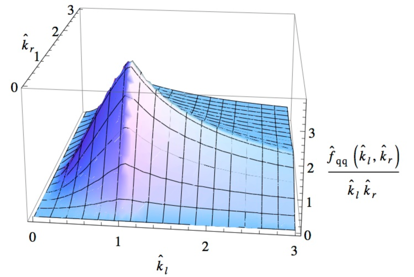
Figure 2: 3D plot of the quark hemisphere contribution to the phase space misalignment correction $\Delta S$.

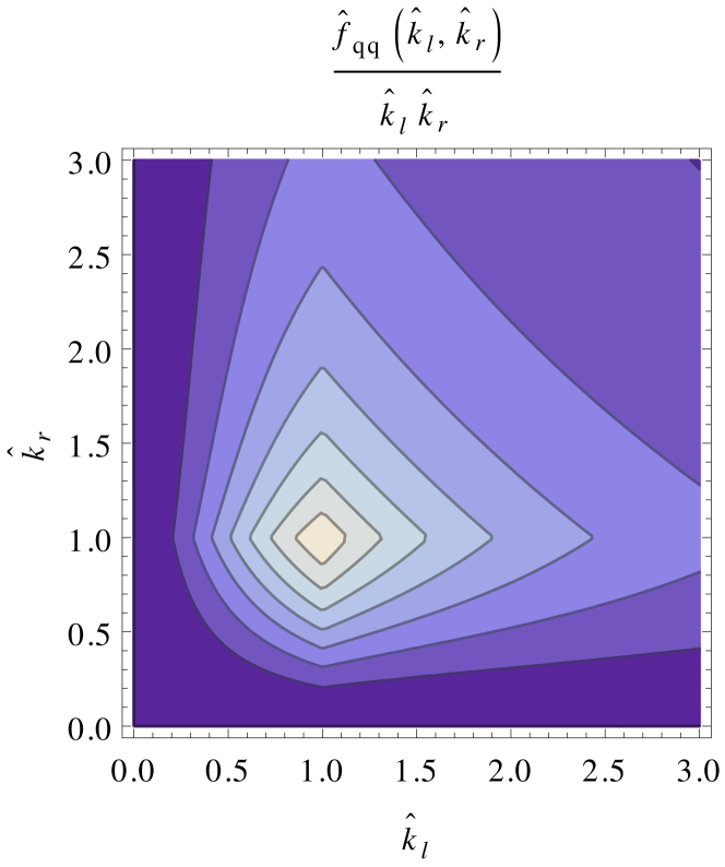
Figure 3: Contour plot of the quark hemisphere contribution to the phase space misalignment correction $\Delta S$.

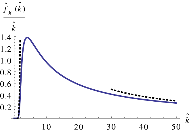
Figure 4: The gluon hemisphere contribution to the phase space misalignment correction $\Delta S$ together with its asymptotic expansions.

We can investigate the asymptotic behavior of the functions $\hat{f}_{qq}$ and $\hat{f}_{g}$ analytically and show the results for very heavy and light quarks explicitly. For $k_{l},k_{r}\ll m$ the expansion of $\hat{f}_{qq}$ yields

$$\hat{f}_{qq}(\hat{k}_{l},\hat{k}_{r})\stackrel{{\scriptstyle\hat{k}_{l},\hat{k}_{r}\ll 1}}{{\longrightarrow}}8\hat{k}_{l}^{3}\hat{k}_{r}^{3}\left[1+\mathcal{O}(\hat{k}_{l}\hat{k}_{r})\right]\,.$$ (35)

This is the only contribution to $\Delta S$ in this limit, since $\hat{f}_{g}$ vanishes here, and gives the suppression of mass effects in the decoupling limit. For $k_{l},k_{r}\gg m$ we get

$$\hat{f}_{qq}\left(\hat{k}_{l},\hat{k}_{r}\right)\stackrel{{\scriptstyle\hat{k}_{l},\hat{k}_{r}\gg 1}}{{\longrightarrow}}f_{qq}\left(\frac{k_{l}}{k_{r}}\right)+\mathcal{O}\left(\frac{1}{\hat{k}_{l}},\frac{1}{\hat{k}_{r}}\right)$$ (36)

with

$$f_{qq}(z)=\frac{16}{3}\,\textrm{ln}(1+z)-\frac{8z(3+3z+2z^{2})}{3(1+z)^{3}}\,\textrm{ln}\,z-\frac{16z}{3(1+z)^{2}}\,.$$ (37)

Note that $f_{qq}(1/z)=f_{qq}(z)$ and $f_{qq}(0)=f_{qq}(\infty)=0$. Turning to $\hat{f}_{g}$ we obtain for $k\gg m$

$$\hat{f}_{g}(\hat{k})\stackrel{{\scriptstyle\hat{k}\gg 1}}{{\longrightarrow}}C_{g}\equiv-\frac{8}{3}+\frac{16\pi^{2}}{9}+\mathcal{O}\left(\frac{1}{\hat{k}}\right)\,.$$ (38)

So the massless limit for the misalignment correction $\Delta S(k_{l},k_{r},m)$ for non-vanishing $k_{l},k_{r}$ reads

$$\mu^{2}\Delta{S}(k_{l}>0,k_{r}>0,m=0)=\frac{\alpha_{s}^{2}C_{F}T_{F}}{16\pi^{2}}\left[\frac{2}{\bar{k}_{l}\bar{k}_{r}}\,f_{qq}\left(\frac{k_{l}}{k_{r}}\right)\right.$$

$$-\left.C_{g}\left(\delta(\bar{k}_{l})\frac{1}{\bar{k}_{r}}+\delta(\bar{k}_{r})\frac{1}{\bar{k}_{l}}\right)\,\right]\,,$$ (39)

The sum of Eq. (V) and the gluon hemisphere contribution for a massless quark $S^{(g)}(k_{l},k_{r},\mu)$ given in Eq. (IV.0.2) correctly reproduces the ${\cal O}(\alpha_{s}^{2}C_{F}T_{F}n_{f})$ massless quark corrections to the hemisphere soft function computed in Ref. Kelley:2011ng for $k_{l},k_{r}>0$. Note that the naive massless limits we obtain for $\hat{f}_{qq}(\hat{k}_{l},\hat{k}_{r})/\hat{k}_{l}\hat{k}_{r}$ and $\hat{f}_{g}(\hat{k})/\hat{k}$ when $k_{l},k_{r}$ are non-vanishing are not integrable at $k_{l}=k_{r}=0$. In the following section we will show, how they recombine into unambiguous distributive expressions.

VI The massless limit of the hemisphere soft function

We now investigate the distributive structure of the ${\cal O}(\alpha_{s}^{2})$ momentum-space double hemisphere soft function $S(k_{l},k_{r},\mu)$ in the massless limit. This issue has not been fully resolved in Refs. Kelley:2011ng ; Hornig:2011iu for the phase space contributions where the quark and antiquark enter different hemispheres. We will find a definite answer for analytic test functions $g(k_{l},k_{r})\neq g(k_{l}/k_{r})$, which have in particular a converging Taylor series around the origin. This is usually the case for test functions which depend on an additional scale, as it is realized for the soft model function $S^{\rm mod}=S^{\rm mod}(k_{l}/\Lambda_{QCD},k_{r}/\Lambda_{QCD})$ which depends intrinsically on the hadronization scale (see also Sec. VIII). The computational rules we can identify concerning the massless limit of the ${\cal O}(\alpha_{s}^{2}C_{F}T_{F})$ massive quark corrections to the soft function can be related to the corresponding massless quark results regularized in dimensional regularization given in Kelley:2011ng ; Hornig:2011iu . They also allow us to determine the complete distributive structure of the pure ${\cal O}(\alpha_{s}^{2}C_{A}C_{F})$ gluonic corrections of the momentum-space double hemisphere soft function.

VI.1 Distributive structure of the ${\cal O}(\alpha_{s}^{2}C_{F}T_{F}n_{f})$ corrections

We first analyze the distributive structure of the ${\cal O}(\alpha_{s}^{2}C_{F}T_{F}n_{f})$ massless quark contributions from the limit $m\to 0$ of the massive quark corrections $S_{m}$ as given in Eq. (29). The massless limit for the gluon hemisphere term $S^{(g)}$ has already been given in Eq. (IV.0.2), so we just have to examine the double cumulant for the phase space misalignment correction $\Delta S$ to derive the distributive structure. Given that the test functions we consider are unique at $k_{l}=k_{r}=0$ we can identify the distributive structures in an unambiguous way. The double cumulant is given by

$$\Delta\mathcal{S}(K_{L},K_{R},m)=\int_{0}^{K_{L}}dk_{l}\int_{0}^{K_{R}}dk_{r}\,\Delta S(k_{l},k_{r},m)$$ (40)

To reach the massless limit we perform an asymptotic expansion for $K_{L,R}\gg m$ both for the quark and gluon hemisphere prescription contributions contained in $\Delta S$. There are in principle many different relevant kinematic regimes for the lightcone components that can contribute. Investigating the integrand $f_{m}(k,q,m)$ given in Eq. (V) and the integration measures for the lightcone components, we find only two relevant regions giving leading $\mathcal{O}(1)$ contributions: (a) $k^{+}\sim k^{-}\sim q^{+}\sim q^{-}\sim m$ and (b) $k^{+}\sim k^{-}\sim q^{+}\sim q^{-}\sim K_{L,R}$. The integration in region (a) appears to be very difficult for an analytic computation, since no expansion is possible for the integrand $f_{m}(k,q,m)$. However, we can take advantage of the fact that the phase space constraints for the gluon and quark hemisphere prescriptions become identical in region (a). This can be seen from Eq. (V), where after integrating in $k_{l}$ and $k_{r}$ the dependence on the large scales $K_{L}$ and $K_{R}$ drops out for small lightcone momenta, which leads to the cancellation between both hemisphere prescriptions. It is therefore sufficient to investigate only the contributions from region (b), where the mass dependence drops from both the integrand and the domain of integration, so that

$$\Delta\mathcal{S}(K_{L},K_{R},m\to 0)=\frac{\alpha_{s}^{2}C_{F}T_{F}}{16\pi^{2}}\int_{0}^{\infty}dq^{-}\int_{0}^{\infty}dk^{+}$$

$$\times\int_{0}^{\infty}dq^{+}\int_{0}^{\infty}dk^{-}\,\theta(q^{+}-q^{-})\,\theta(k^{-}-k^{+})$$

$$\times\left[\theta(K_{R}-q^{-})\,\theta(K_{L}-k^{+})\right.$$

$$-\theta(k^{+}+q^{+}-k^{-}-q^{-})\,\theta(K_{R}-q^{-}-k^{-})\,\theta(K_{L})$$

$$-\left.\theta(k^{-}+q^{-}-k^{+}-q^{+})\,\theta(K_{L}-q^{+}-k^{+})\,\theta(K_{R})\right]$$

$$\times f_{0}(k^{+},k^{-},q^{+},q^{-})\,,$$ (41)

with the massless integrand

$$f_{0}(k^{+},k^{-},q^{+},q^{-})= \frac{16}{(k^{+}+q^{+})^{2}(k^{-}+q^{-})^{2}}$$

$$\times\frac{q^{+}q^{-}+k^{+}k^{-}}{q^{+}k^{-}-k^{+}q^{-}}\,.$$ (42)

The remaining integrations can be performed separately for the contributions from the quark and gluon hemisphere prescriptions with an additional IR regulator, where the IR divergence comes from the region where all momenta are small. We have chosen a cutoff regulator for one of the lightcone components and observed that it properly cancels in the final expression in the difference between the two hemisphere contributions. This cancellation takes place since the IR divergences in the quark and gluon hemisphere prescriptions match. The final outcome reads

$$\Delta\mathcal{S}(K_{L},K_{R})= \,\frac{\alpha_{s}^{2}C_{F}T_{F}}{16\pi^{2}}\left[2\mathcal{F}_{qq}\left(\frac{K_{L}}{K_{R}}\right)-\frac{88}{9}+\frac{104}{27}\pi^{2}\right.$$

$$+\left.\frac{32}{3}\zeta(3)\right]$$ (43)

with the function

$$\mathcal{F}_{qq}(z)= \,16\,\textrm{Li}_{3}(-z)-\frac{16}{3}\,\textrm{ln}\,z\,\textrm{Li}_{2}(-z)+\frac{8\pi^{2}}{9}\textrm{ln}\,z$$

$$-\frac{4(1-z)}{3(1+z)}\,\textrm{ln}\,z\,,$$ (44)

which is symmetric with respect to $z\leftrightarrow 1/z$.

The result given in Eq. (VI.1) can be written as an integration over distributions in the variables $k_{l}$ and $k_{r}$. Away from the origin we should reproduce the structure in Eq. (V) with (37) and (38). We further anticipate that the structure $[\frac{1}{k_{l}}]_{+}[\frac{1}{k_{r}}]_{+}f_{qq}(k_{l}/k_{r})$ is part of the final answer and compute its contribution to the cumulant using the fact that $f_{qq}(0)=0$: ($\bar{K}_{L}=K_{L}/\mu$ etc.)

$$\int^{\bar{K}_{R}}_{0}d\bar{k}_{r}\left[\frac{1}{\bar{k}_{r}}\right]_{+}\int^{\bar{K}_{L}}_{0}d\bar{k}_{l}\left[\frac{1}{\bar{k}_{l}}\right]_{+}f_{qq}\left(\frac{\bar{k}_{l}}{\bar{k}_{r}}\right)$$

$$=\int^{\bar{K}_{R}}_{0}d\bar{k}_{r}\left[\frac{1}{\bar{k}_{r}}\right]_{+}\int^{\frac{\bar{K}_{L}}{\bar{k}_{r}}}_{0}\frac{f_{qq}(z)}{z}\,dz$$

$$=\int^{\frac{K_{R}}{K_{L}}}_{0}dx\frac{1}{x}\left(\int^{1}_{0}dz\,\frac{f_{qq}(z/x)}{z}-C_{qq}\right)+C_{qq}\textrm{ln}\,\bar{K}_{R}$$

$$\equiv\mathcal{F}_{qq}\left(\frac{K_{L}}{K_{R}}\right)+\frac{1}{2}C_{qq}\left(\textrm{ln}\,\bar{K}_{R}+\textrm{ln}\,\bar{K}_{L}\right)\,,$$ (45)

where

$$C_{qq}\equiv\int^{\infty}_{0}\frac{f_{qq}(z)}{z}\,dz=-\frac{8}{3}+\frac{16\pi^{2}}{9}=C_{g}\,.$$ (46)

Note that the calculation is unambiguous owing to the property $f_{qq}(0)=f_{qq}(\infty)=0$. Moreover, the order of the integrations can be exchanged, since $f_{qq}(z)=f_{qq}(1/z)$. The result of Eq. (46) allows the additional logarithms in the final equality of Eq. (VI.1) to be recombined with $C_{g}$ into distributions that yield the correct cumulant in Eq. (VI.1) compatible with Eq. (V). This gives the desired distributive expression for the phase space misalignment correction:

$$\mu^{2}\Delta S(k_{l},k_{r},\mu)=\frac{\alpha_{s}^{2}C_{F}T_{F}}{16\pi^{2}}\left\{\delta(\bar{k}_{l})\delta(\bar{k}_{r})\left[-\frac{44}{9}+\frac{52}{27}\pi^{2}\right.\right.$$

$$+\left.\frac{16}{3}\zeta(3)\right]+\delta(\bar{k}_{l})\left[\frac{\theta(\bar{k}_{r})}{\bar{k}_{r}}\right]_{+}\left[\frac{8}{3}-\frac{16}{9}\pi^{2}\right]$$

$$\left.+\left[\frac{\theta(\bar{k}_{l})}{\bar{k}_{l}}\right]_{+}\left[\frac{\theta(\bar{k}_{r})}{\bar{k}_{r}}\right]_{+}f_{qq}\left(\frac{k_{l}}{k_{r}}\right)+(k_{l}\leftrightarrow k_{r})\right\}\,.$$ (47)

with the term $f_{qq}$ given in Eq. (37). Combining this result with Eq. (IV.0.2) we obtain the entire distributive structure of the ${\cal O}(\alpha_{s}^{2}C_{F}T_{F}n_{f})$ massless quark corrections to the momentum-space double hemisphere soft function valid for all $k_{l},k_{r}\geq 0$,

$$\mu^{2}S_{n_{f}}(k_{l},k_{r},\mu)=\mu^{2}Z_{S,n_{f}}(k_{l},k_{r},\mu)+\frac{\alpha_{s}^{2}C_{F}T_{F}n_{f}}{16\pi^{2}}$$

$$\times\left\{\delta(\bar{k}_{l})\,\delta(\bar{k}_{r})\left[-\frac{68}{81}+\frac{37}{27}\pi^{2}+\frac{28}{9}\zeta(3)\right]\right.$$

$$+\delta(\bar{k}_{l})\left[\frac{\theta(\bar{k}_{r})}{\bar{k}_{r}}\right]_{+}\left[-\frac{152}{27}-\frac{8\pi^{2}}{9}\right]$$

$$+\delta(\bar{k}_{l})\left[\frac{\theta(\bar{k}_{r})\textrm{ln}\,\bar{k}_{r}}{\bar{k}_{r}}\right]_{+}\frac{160}{9}-\delta(\bar{k}_{l})\left[\frac{\theta(\bar{k}_{r})\textrm{ln}^{2}\bar{k}_{r}}{\bar{k}_{r}}\right]_{+}\frac{32}{3}$$

$$+\left.\left[\frac{\theta(\bar{k}_{l})}{\bar{k}_{l}}\right]_{+}\left[\frac{\theta(\bar{k}_{r})}{\bar{k}_{r}}\right]_{+}f_{qq}\left(\frac{k_{l}}{k_{r}}\right)+(k_{l}\leftrightarrow k_{r})\right\}\,,$$ (48)

where we have included the massless flavor number $n_{f}$. The UV divergences which are absorbed into the soft function renormalization factor read

$$Z_{S,n_{f}}(k_{l},k_{r},\mu)=n_{f}Z_{S,m}(k_{l},k_{r},\mu)$$ (49)

with $Z_{S,m}(k_{l},k_{r},\mu)$ given in Eq. (IV.0.2). As already mentioned in Sec. V, this result agrees for $k_{l},k_{r}>0$ with the naive $\epsilon\to 0$ expansion of the corresponding $d\neq 4$ result given in Eq. (31) of Ref. Kelley:2011ng .

Interestingly, from the result in Eq. (VI.1) we can now also establish unambiguous rules for the $\epsilon\to 0$ limit of the $d\neq 4$ results for the ${\cal O}(\alpha_{s}^{2})$ corrections to the momentum space double hemisphere discussed in Refs. Kelley:2011ng ; Hornig:2011iu valid for all $k_{l},k_{r}\geq 0$: Writing $f_{n_{f}}(z,\epsilon)=f_{n_{f}}^{(0)}(z)+\epsilon f_{n_{f}}^{(1)}(z)+\dots$ for the opposite hemisphere correction given in Eqs. (28), (A4) and (A5) of Ref. Kelley:2011ng , the dictionary from their $d$-dimensional expression resulting from Eq. (VI.1) reads

$$\frac{\mu^{4\epsilon}}{(k_{l}k_{r})^{1+2\epsilon}}f_{n_{f}}\left(\frac{k_{l}}{k_{r}},\epsilon\right)$$

$$\stackrel{{\scriptstyle\epsilon\to 0}}{{\longrightarrow}}\,\delta(\bar{k}_{l})\,\delta(\bar{k}_{r})\left[-\frac{1}{4\epsilon}\int^{\infty}_{0}\frac{dz}{z}\left(f_{n_{f}}^{(0)}(z)+\epsilon f_{n_{f}}^{(1)}(z)\right)\right]$$

$$+\left[\frac{\theta(\bar{k}_{l})}{\bar{k}_{l}}\right]_{+}\left[\frac{\theta(\bar{k}_{r})}{\bar{k}_{r}}\right]_{+}f_{n_{f}}^{(0)}\left(\frac{k_{l}}{k_{r}}\right)+\mathcal{O}(\epsilon)$$ (50)

with $f_{n_{f}}^{(0)}(z)=2f_{qq}(z)$, see Eq. (37). Note that due to the symmetry $k_{l}\leftrightarrow k_{r}$ ($f^{(n)}_{n_{f}}(z)=f^{(n)}_{n_{f}}(1/z)$) and $f_{n_{f}}^{(n)}(0)=f_{n_{f}}^{(n)}(\infty)=0$ (for $n=0,1,2,...$) one has

$$\int^{\infty}_{0}dz\,\frac{\textrm{ln}\,z}{z}\,f^{(n)}_{n_{f}}(z)=0\,,$$ (51)

so that corresponding contributions do not arise in Eq. (VI.1). The expansion given in Eq. (VI.1) applies if $f_{n_{f}}\left(0,\epsilon\right)=f_{n_{f}}\left(\infty,\epsilon\right)=0$. It is straightforward to generalize to the case $f\left(0,\epsilon\right)=f\left(\infty,\epsilon\right)\neq 0$. In this situation we can define a new function $\tilde{f}\left(z,\epsilon\right)=f\left(z,\epsilon\right)-f\left(0,\epsilon\right)$, for which we can apply the rule in Eq. (VI.1). For the remaining constant $f\left(0,\epsilon\right)$ we can expand in $k_{l}$ and $k_{r}$ multiplicatively in the usual way generating products of additional single variable distributions in $k_{l}$ and $k_{r}$.

VI.2 Result for the full ${\cal O}(\alpha_{s}^{2})$ momentum-space double hemisphere soft function

We are now in the position to write down the complete distributive expression for the momentum-space double hemisphere soft function at ${\cal O}(\alpha_{s}^{2})$ accounting for all gluonic, the massless as well as massive quark corrections. The results for the pure gluonic corrections can be derived with the help of the expansion rule (VI.1) and the results in Kelley:2011ng ; Hornig:2011iu . The different structures for the unrenormalized soft function in the scheme, where the strong coupling evolves with the $n_{f}$ massless and one massive flavor ($\alpha_{s}=\alpha_{s}^{(n_{f}+1)}$), read

$$S(k_{l},k_{r},\mu)= \,S_{C_{F}}(k_{l},k_{r},\mu)+S_{C_{A}}(k_{l},k_{r},\mu)$$

$$+S_{n_{f}}(k_{l},k_{r},\mu)+S_{m}(k_{l},k_{r},m,\mu)\,,$$ (52)

where $S_{n_{f}}(k_{l},k_{r},\mu)$ is the massless quark correction given in Eq. (VI.1) and $S_{m}(k_{l},k_{r},m,\mu)$ are the massive quark corrections in Eq. (29). Using the results from Kelley:2011ng for the $C_{F}C_{A}$-part and applying (VI.1) we obtain

$$\mu^{2}S_{C_{A}}(k_{l},k_{r},\mu)=\mu^{2}Z_{S,C_{A}}(k_{l},k_{r},\mu)+\frac{\alpha_{s}^{2}C_{F}C_{A}}{16\pi^{2}}$$

$$\times\left\{\delta(\bar{k}_{l})\,\delta(\bar{k}_{r})\left[-\frac{1016}{81}-\frac{335}{108}\pi^{2}-\frac{77}{9}\zeta(3)+\frac{26}{45}\pi^{4}\right]\right.$$

$$+\delta(\bar{k}_{l})\left[\frac{\theta(\bar{k}_{r})}{\bar{k}_{r}}\right]_{+}\left[\frac{772}{27}+\frac{22\pi^{2}}{9}-36\zeta(3)\right]$$

$$-\delta(\bar{k}_{l})\left[\frac{\theta(\bar{k}_{r})\textrm{ln}\,\bar{k}_{r}}{\bar{k}_{r}}\right]_{+}\frac{536}{9}+\delta(\bar{k}_{l})\left[\frac{\theta(\bar{k}_{r})\textrm{ln}^{2}\bar{k}_{r}}{\bar{k}_{r}}\right]_{+}\frac{88}{3}$$

$$+\left[\frac{\theta(\bar{k}_{l})}{\bar{k}_{l}}\right]_{+}\left[\frac{\theta(\bar{k}_{r})}{\bar{k}_{r}}\right]_{+}\left[\frac{4\pi^{2}}{3}+f_{gg}\left(\frac{k_{l}}{k_{r}}\right)\right]$$

$$+(k_{l}\leftrightarrow k_{r})\bigg{\}}$$ (53)

with

$$f_{gg}(z)=\,4\,\textrm{ln}^{2}(1+z)-4\,\textrm{ln}(1+z)\,\textrm{ln}\,z-\frac{44}{3}\,\textrm{ln}(1+z)$$

$$+\frac{4z(12+21z+11z^{2})}{3(1+z)^{3}}\,\textrm{ln}\,z+\frac{8z}{3(1+z)^{2}}\,$$ (54)

satisfying $f_{gg}(z)=f_{gg}(1/z)$ and $f_{gg}(0)=0$. The UV divergent contribution which adds to the soft function renormalization constant reads

$$\mu^{2}Z_{S,C_{A}}(k_{l},k_{r},\mu)=\frac{\alpha_{s}^{2}C_{F}C_{A}}{16\pi^{2}}\delta(\bar{k}_{l})\left\{\delta(\bar{k}_{r})\left[\frac{11}{2\epsilon^{3}}\right.\right.$$

$$+\left.\frac{1}{\epsilon^{2}}\left(-\frac{67}{18}+\frac{\pi^{2}}{6}\right)+\frac{1}{\epsilon}\left(-\frac{202}{27}+\frac{11\pi^{2}}{36}+7\zeta(3)\right)\right]$$

$$\left.+\,\left[\frac{\theta(\bar{k}_{r})}{\bar{k}_{r}}\right]_{+}\left[-\frac{22}{3\epsilon^{2}}+\frac{1}{\epsilon}\left(\frac{134}{9}-\frac{2\pi^{2}}{3}\right)\right]\right\}+(k_{l}\leftrightarrow k_{r})\,.$$ (55)

To obtain this result we have rewritten the function $f_{C_{A}}(z,\epsilon)$ given in Eq. (17) of Ref. Kelley:2011ng as $f_{C_{A}}(z,\epsilon)=\tilde{f}_{C_{A}}(z,\epsilon)+f_{C_{A}}(0,\epsilon)$ and proceeded as described at the end of Sec. VI.1 for the expansion in terms of distributions. We have defined $2f_{gg}(z)\equiv f_{C_{A}}^{(0)}(z)-f_{C_{A}}^{(0)}(0)$ with $f_{C_{A}}^{(0)}(z)$ given in Eq. (A1) of Ref. Kelley:2011ng and $f_{C_{A}}^{(0)}(0)\equiv 8\pi^{2}/3$.

The distributive structure of the remaining gluonic $C_{F}^{2}$-corrections is already known completely as it can be obtained from the exponentiation of the one-loop result in position space Hoang:2008fs , and its $k_{l}$- and $k_{r}$-dependence factorizes without any subtleties. For completeness we also give the result for the $\mathcal{O}(\alpha_{s}^{2}C_{F}^{2})$ corrections to the unrenormalized soft function,

$$\mu^{2}S_{C_{F}}(k_{l},k_{r},\mu)=\mu^{2}Z_{S,C_{F}}(k_{l},k_{r},\mu)+\frac{\alpha_{s}^{2}C_{F}^{2}}{16\pi^{2}}$$

$$\times\left\{-\delta(\bar{k}_{l})\delta(\bar{k}_{r})\frac{11\pi^{4}}{180}+\delta(\bar{k}_{l})\left[\frac{\theta(\bar{k}_{r})}{\bar{k}_{r}}\right]_{+}64\zeta(3)\right.$$

$$-\delta(\bar{k}_{l})\left[\frac{\theta(\bar{k}_{r})\textrm{ln}\,\bar{k}_{r}}{\bar{k}_{r}}\right]_{+}\frac{40\pi^{2}}{3}+\delta(\bar{k}_{l})\left[\frac{\theta(\bar{k}_{r})\textrm{ln}^{3}\bar{k}_{r}}{\bar{k}_{r}}\right]_{+}32$$

$$+\left.\left[\frac{\theta(\bar{k}_{l})\textrm{ln}\,\bar{k}_{l}}{\bar{k}_{l}}\right]_{+}\left[\frac{\theta(\bar{k}_{r})\textrm{ln}\,\bar{k}_{r}}{\bar{k}_{r}}\right]_{+}32+(k_{l}\leftrightarrow k_{r})\right\}\,$$ (56)

with

$$\mu^{2}Z_{S,C_{F}}(k_{l},k_{r},\mu)=\frac{\alpha_{s}^{2}C_{F}^{2}}{16\pi^{2}}\left\{\delta(\bar{k}_{l})\delta(\bar{k}_{r})\left[\frac{4}{\epsilon^{4}}-\frac{2\pi^{2}}{\epsilon^{2}}\right.\right.$$

$$-\left.\frac{32\zeta(3)}{\epsilon}\right]+\delta(\bar{k}_{l})\left[\frac{\theta(\bar{k}_{r})}{\bar{k}_{r}}\right]_{+}\left[-\frac{16}{\epsilon^{3}}+\frac{20\pi^{2}}{3\epsilon}\right]$$

$$+\delta(\bar{k}_{l})\left[\frac{\theta(\bar{k}_{r})\textrm{ln}\,\bar{k}_{r}}{\bar{k}_{r}}\right]_{+}\frac{48}{\epsilon^{2}}-\delta(\bar{k}_{l})\left[\frac{\theta(\bar{k}_{r})\textrm{ln}^{2}\bar{k}_{r}}{\bar{k}_{r}}\right]_{+}\frac{48}{\epsilon}$$

$$+\left[\frac{\theta(\bar{k}_{l})}{\bar{k}_{l}}\right]_{+}\left[\frac{\theta(\bar{k}_{r})}{\bar{k}_{r}}\right]_{+}\frac{8}{\epsilon^{2}}$$

$$\left.-\left[\frac{\theta(\bar{k}_{l})}{\bar{k}_{l}}\right]_{+}\left[\frac{\theta(\bar{k}_{r})\textrm{ln}\,\bar{k}_{r}}{\bar{k}_{r}}\right]_{+}\frac{32}{\epsilon}+(k_{l}\leftrightarrow k_{r})\right\}$$ (57)

for the UV divergent terms. We have checked analytically that the cumulants generated by Eqs. (VI.1), (VI.2), (VI.2) agree with the expressions given in Eqs. (50) and (53) of Ref. Kelley:2011ng and Eqs. (3.36)-(3.43) of Ref. Hornig:2011iu . Furthermore, we have found agreement to the resulting expressions for the corresponding ${\cal O}(\alpha_{s}^{2})$ corrections to the thrust soft function given in Eq. (41) of Ref. Kelley:2011ng (see also Monni:2011gb ), and furthermore to the heavy jet mass constant in Eq. (42) of Ref. Kelley:2011ng . Moreover, the position space representation of the massless quark and gluon corrections, i.e. the Fourier transformations of Eqs. (VI.1), (VI.2), (VI.2), agree with the ones given in Eqs. (3.30)-(3.35) of Ref. Hornig:2011iu .

VII Projection onto thrust

From the massive quark corrections to the ${\cal O}(\alpha_{s}^{2})$ double hemisphere soft function we can derive the corresponding soft function corrections for a few other event shape variables. Here we investigate the most prominent projection, namely thrust. We define the thrust variable by

$$\tau=1-T\,=\,1-\sum_{i}\frac{|\vec{n}\cdot\vec{p}_{i}|}{\sum_{j}|E_{j}|}\,=\,1-\sum_{i}\frac{|\vec{n}\cdot\vec{p}_{i}|}{Q}\,,$$ (58)

where $\vec{n}$ is the thrust axis and the sum is performed over all final state particles with momenta $\vec{p}_{i}$ and energies $E_{i}$. The partonic soft function for the thrust distribution can be easily obtained from the linear relation

$$\tau=\frac{M_{l}^{2}+M_{r}^{2}}{Q^{2}}+\mathcal{O}\left(\frac{M_{l,r}^{4}}{Q^{4}}\right)$$ (59)

in the dijet limit, which yields

$$S_{\tau}(\ell,m,\mu)=\int dk_{r}\,dk_{l}\,\delta(\ell-k_{r}-k_{l})\,S(k_{r},k_{l},m,\mu)\,.$$ (60)

We can split the ${\cal O}(\alpha_{s}^{2}C_{F}T_{F})$ massive quark corrections to the partonic thrust soft function into

$$S_{\tau,m}(\ell,m,\mu)= \,Z_{S,\tau}(\ell,\mu)+S^{(g)}_{\tau,\rm virt}(\ell,m,\mu)$$

$$+S^{(g)}_{\tau,\rm real}(\ell,m,\mu)+\Delta S_{\tau}(\ell,m)\,,$$ (61)

according to Eqs. (IV.0.2) and (29). In Eq. (61) the term $S^{(g)}_{\tau,\rm virt}$ ($S^{(g)}_{\tau,\rm real}$) corresponds to the virtual (real) massive quark radiation piece coming from the gluon hemisphere prescription, while $\Delta S_{\tau}(\ell,m)$ is the finite phase space misalignment correction due to the physical quark hemisphere prescription. These are related to the corresponding double hemisphere results of Eqs. (IV.0.2), (IV.0.2) and (V). For the gluon hemisphere contributions the convolution according to Eq. (60) is straightforward and we obtain ($\bar{\ell}=\ell/\mu$)

$$\mu\,S^{(g)}_{\tau,\rm virt}(\ell,m,\mu)=\frac{\alpha_{s}^{2}C_{F}T_{F}}{16\pi^{2}}\left\{\delta(\bar{\ell})\left[-\frac{8}{9}L_{m}^{3}-\frac{40}{9}L_{m}^{2}\right.\right.$$

$$+\left.\left(-\frac{448}{27}+\frac{8\pi^{2}}{9}\right)L_{m}-\frac{656}{27}+\frac{10\pi^{2}}{27}+\frac{56}{9}\zeta(3)\right]$$

$$+\left[\frac{\theta(\bar{\ell})}{\bar{\ell}}\right]_{+}\left[\frac{16}{3}L_{m}^{2}+\frac{160}{9}L_{m}+\frac{448}{27}\right]$$

$$-\left.\left[\frac{\theta(\bar{\ell})\textrm{ln}\,\bar{\ell}}{\bar{\ell}}\right]_{+}\frac{64}{3}L_{m}\right\}\,,$$ (62)

$$\mu\,S^{(g)}_{\tau,\rm real}(\ell,m,\mu)=\frac{\alpha_{s}^{2}C_{F}T_{F}}{16\pi^{2}}\,\theta(\ell-2m)\,\frac{2}{\bar{\ell}}R\left(\sqrt{1-\frac{4m^{2}}{\ell^{2}}}\right)\,,$$ (63)

where the function $R\left(w\right)$ is defined in Eq. (IV.0.2). The UV divergences that contribute to the soft function renormalization constant read

$$\mu\,Z_{S,\tau}(\ell,\mu)=\frac{\alpha_{s}^{2}C_{F}T_{F}}{16\pi^{2}}\left\{\delta(\bar{\ell})\left[-\frac{4}{\epsilon^{3}}+\frac{20}{9\epsilon^{2}}\right.\right.$$

$$\left.+\left.\frac{1}{\epsilon}\left(\frac{112}{27}-\frac{2\pi^{2}}{9}\right)\right]+\left[\frac{\theta(\bar{\ell})}{\bar{\ell}}\right]_{+}\left[\frac{16}{3\epsilon^{2}}-\frac{80}{9\epsilon}\right]\right\}\,.$$ (64)

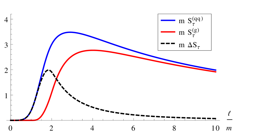
Figure 5: The contributions to the thrust soft function from the opposite hemisphere phase space, for the quark hemisphere prescription $m\,S^{(qq)}(\ell,m)$ (blue), gluon hemisphere prescription $m\,S^{(g)}(\ell,m)$ (red) and the difference giving $m\,\Delta S_{\tau}(\ell,m)$ (black, dashed).

The contribution from the phase space misalignment correction $\Delta S_{\tau}(\ell,m)$ can be written analogously to Eq. (V),

$$\Delta S_{\tau}(\ell,m)=\frac{\alpha_{s}^{2}C_{F}T_{F}}{16\pi^{2}}\int dq^{-}\int dk^{+}\int dq^{+}\int dk^{-}$$

$$\times\theta(k^{-}-k^{+})\,\theta(q^{+}-q^{-})\,\theta(k^{+}k^{-}-m^{2})\,\theta(q^{+}q^{-}-m^{2})$$

$$\times\,\theta(k^{-}+k^{+})\,\theta(q^{+}+q^{-})\left[\delta(\ell-k^{+}-q^{-})\right.$$

$$-\theta(k^{-}+q^{-}-k^{+}-q^{+})\,\delta(\ell-k^{+}-q^{+})$$

$$-\left.\theta(k^{+}+q^{+}-k^{-}-q^{-})\,\delta(\ell-k^{-}-q^{-})\right]$$

$$\times f_{m}(k^{+},k^{-},q^{+},q^{-},m)$$ (65)

where $f_{m}$ has been given in Eq. (V). It can be calculated numerically using the Cuba library Hahn:2004fe . For large values of $\ell/m$ $\Delta S_{\tau}(\ell,m)$ involves strong cancellations in the difference between its quark and gluon hemisphere contributions (see also Eq. (A)), which can lead to numerical instabilities. This is illustrated in Fig. 5 where $\Delta S_{\tau}(\ell,m)$ is shown together with its two contributions from both prescriptions. An alternative way to compute $\Delta S_{\tau}(\ell,m)$ for large values of $\ell/m$ can be achieved by evaluating the cumulant, where the quark and gluon hemisphere contributions can be combined prior to integration, and by differentiating numerically afterwards (see the appendix).

In the massless limit $\Delta S_{\tau}$ becomes a delta function and gives ($\bar{\ell}=\ell/\mu$)

$$\mu\,\Delta S_{\tau}(\ell,m)\stackrel{{\scriptstyle m\rightarrow 0}}{{\longrightarrow}}\frac{\alpha_{s}^{2}C_{F}T_{F}}{16\pi^{2}}\delta(\bar{\ell})\left\{-\frac{64}{9}+\frac{104\pi^{2}}{27}-\frac{64\zeta(3)}{3}\right\}\,.$$ (66)

Together with the massless limits of Eqs. (62), (63) this yields

$$\mu\,S_{\tau,m}(\ell,m\rightarrow 0,\mu)=\mu\,Z_{S,\tau}(\ell,\mu)+\frac{\alpha_{s}^{2}C_{F}T_{F}}{16\pi^{2}}$$

$$\times\left\{\delta(\bar{\ell})\left[\frac{80}{81}+\frac{74\pi^{2}}{27}-\frac{232}{9}\zeta(3)\right]+\left[\frac{\theta(\bar{\ell})}{\bar{\ell}}\right]_{+}\left[-\frac{448}{27}\right.\right.$$

$$\left.+\left.\frac{16\pi^{2}}{9}\right]+\left[\frac{\theta(\bar{\ell})\,\textrm{ln}\,\bar{\ell}}{\bar{\ell}}\right]_{+}\frac{320}{9}-\left[\frac{\theta(\bar{\ell})\,\textrm{ln}^{2}\bar{\ell}}{\bar{\ell}}\right]_{+}\frac{64}{3}\right\}\,,$$ (67)

which is the result known for one massless quark flavor Kelley:2011ng ; Monni:2011gb .

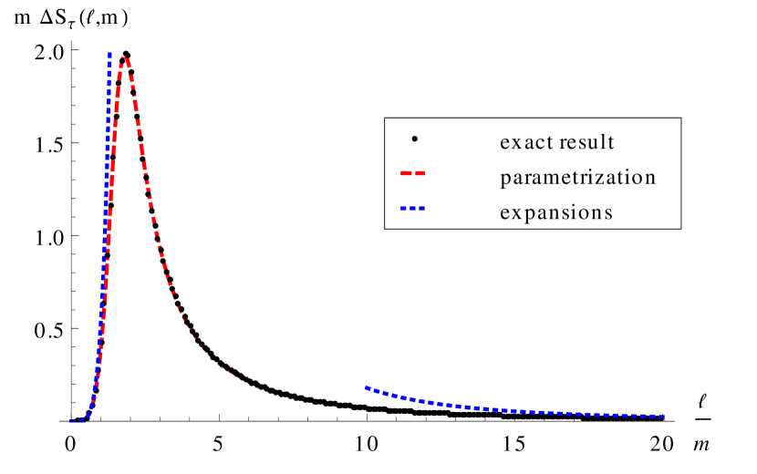
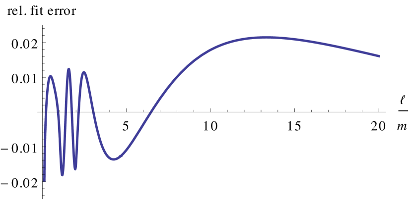
Figure 6: Above: Phase space misalignment correction $m\,\Delta S_{\tau}(\ell,m)$ (black dots) together with the fit of Eq. (VII) (red,dashed) and its asymptotic expansions (blue,dotted), normalized by the prefactor $\alpha_{s}^{2}C_{F}T_{F}/16\pi^{2}$. The fit is almost indistinguishable from the exact function. Below: The relative difference between fit and exact function for $\Delta S_{\tau}(\ell,m)$ (compared to an interpolation).

We aim at providing a parametrization of $\Delta S_{\tau}(\ell,m)$, which can be used for a numerical analysis of mass effects for the thrust distribution. For this purpose, we perform asymptotic expansions for small and large ratios $\ell/m$. First we consider the expansion for small thrust momenta or large quark masses, which can be obtained from integrating Eq. (35), yielding

$$\mu\,\Delta S_{\tau}(\ell,m)\stackrel{{\scriptstyle\ell\ll m}}{{\longrightarrow}}\frac{\alpha_{s}^{2}C_{F}T_{F}}{16\pi^{2}}\,\frac{1}{\bar{\ell}}\frac{8\ell^{6}}{15m^{6}}\left[1+\mathcal{O}\left(\frac{\ell^{2}}{m^{2}}\right)\right]\,.$$ (68)

Note that there is no threshold, below which this contribution vanishes. The expansion for large thrust momenta is more challenging and described in the appendix. The final result reads

$$\mu\,\Delta S_{\tau}(\ell,m)\stackrel{{\scriptstyle\ell\gg m}}{{\longrightarrow}}\frac{\alpha_{s}^{2}C_{F}T_{F}}{16\pi^{2}}\frac{1}{\bar{\ell}}\frac{m^{2}}{\ell^{2}}\left[8\textrm{ln}^{2}\left(\frac{m^{2}}{\ell^{2}}\right)\right.$$

$$+\left.80\textrm{ln}\left(\frac{m^{2}}{\ell^{2}}\right)+\frac{640}{3}+\frac{292\pi^{2}}{45}+32\pi\right]\left[1+\mathcal{O}\left(\frac{m}{\ell}\right)\right]\,.$$ (69)

A possible parametrization of $\Delta S_{\tau}(\ell)$ can be given by a Padé-type rational function multiplying some logarithmic terms. We adopt an analytic ansatz that is capable of yielding the asymptotic behaviors of Eqs. (68) and  (VII) and has a finite normalization,

$$\Delta S_{\tau}(x=\ell/m)\bigg{|}_{\rm fit}=\frac{\alpha_{s}^{2}C_{F}T_{F}}{16\pi^{2}}\,\frac{1}{m}$$

$$\times\frac{x^{5}\left(a\,\textrm{ln}^{2}\left(1+x^{2}\right)+b\,\textrm{ln}\left(1+x^{2}\right)+c\right)}{dx^{8}+ex^{7}+fx^{6}+gx^{4}+hx^{3}+jx^{2}+1}\,.$$ (70)

with $a=8d$, $b=-80d$, $c=8/15$ and $d=6/(2400+360\pi+73\pi^{2})$ fixed by requiring the correct asymptotic behavior. The remaining 5 parameters were obtained using a $\chi^{2}$-fit with the constraint of satisfying the correct normalization corresponding to the massless analytic limit given in Eq. (66). We get

$$e=0.0117\,,\,f=0.100\,,\,g=-0.502\,,$$

$$h=0.747\,,\,j=-0.180\,.$$ (71)

These fitted values correspond to a local minimum of the $\chi^{2}$-function which has the feature that the relative error of the fit function to the exact function does not exceed $3\%$ anywhere, and is around $1\%$ in the peak region, where the bulk of the contribution arises. The exact and fitted results together with the asymptotic expansions are displayed in Fig. 6.

The three components of the $\mathcal{O}(\alpha_{s}^{2}C_{F}T_{F})$ massive quark corrections to the renormalized thrust soft function, their sum and the massless limit are displayed together with the cumulants in Fig. 7 for $\mu=m$ as a function of $\ell/m$ and $L/m$, respectively. We see that the phase space misalignment correction represents a relatively small contribution.

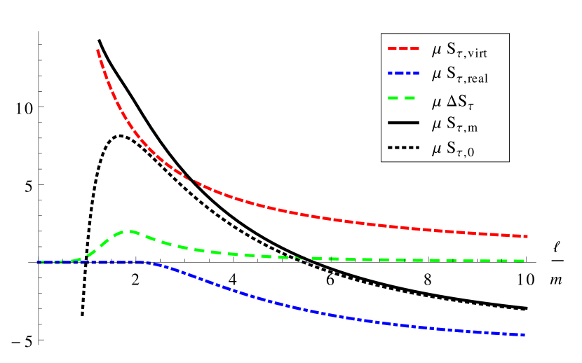
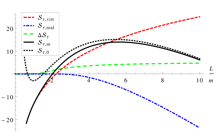
Figure 7: Plots of the massive quark contributions to the thrust soft function (upper panel) and its cumulant (lower panel) for $\mu=m$, normalized by the prefactor $\alpha_{s}^{2}C_{F}T_{F}/16\pi^{2}$. $S_{\tau,{\rm virt}}$, $S_{\tau,{\rm real}}$ and $\Delta S_{\tau}$ denote the virtual, real radiation and phase space misalignment contributions described in the text, $S_{\tau,m}$ is their sum, i.e. the full massive contribution, and $S_{\tau,0}$ is the massless contribution. The corresponding descriptions also hold for the cumulant terms.

VIII Renormalon subtractions with secondary massive particles

The complete soft function is a convolution of the partonic soft function, describing perturbative corrections at the soft scale, and the nonperturbative hadronic soft function Hoang:2007vb . Using dimensional regularization and the $\overline{\rm MS}$ scheme for UV divergences entails that the interface between perturbative and nonperturbative contributions suffers from IR renormalon problems. These are related to contributions from very small momenta entering in the perturbative computations and lead to factorially enhanced coefficients of the high-order perturbation series which can render the determination of the nonperturbative parameters in the hadronic soft function unstable. In the gap formalism for the soft function Hoang:2007vb ; Hoang:2008fs one can eliminate the renormalon problem for the leading ${\cal O}(\Lambda_{\rm QCD})$ power correction that arises in the operator production expansion (OPE) of the soft function for $k_{l}\sim k_{r}\gg\Lambda_{\rm QCD}$. This is achieved through a perturbative subtraction that eliminates order-by-order the leading power IR sensitivity of the partonic soft function. The name of the gap formalism arises from the fact that the subtraction is physically related to the minimal hadronic energy deposit $\Delta\sim\Lambda_{\rm QCD}$ in the two hemispheres and can thus be implemented through a shift in the momentum arguments $k_{l}$ and $k_{r}$ of the partonic soft function. So the subtracted partonic soft function, which is free of the ${\cal O}(\Lambda_{\rm QCD})$ renormalon has the form Hoang:2007vb

$$S_{\rm part}(k_{l}-\delta(R,\mu),k_{r}-\delta(R,\mu),\mu)\,,$$ (72)

where $\delta(R,\mu)$ is a properly defined perturbative series. A very convenient definition is Hoang:2008fs

$$\delta(R,\mu)=\frac{Re^{\gamma_{E}}}{2}\left(\frac{d}{d\,\textrm{ln}(ix_{l})}\right.$$

$$+\left.\frac{d}{d\,\textrm{ln}(ix_{r})}\right)\left.\textrm{ln}\,\tilde{S}_{\rm{part}}(x_{l},x_{r},\mu)\right|_{x_{l}=x_{r}=(iRe^{\gamma_{E}})^{-1}},$$ (73)

where $\tilde{S}$ is the configuration space partonic soft function

$$\tilde{S}_{\rm{part}}(x_{l},x_{r},\mu)=\int dk_{l}\,dk_{r}\,S_{\rm part}(k_{l},k_{r},\mu)\,e^{-ik_{l}x_{l}}e^{-ik_{r}x_{r}}\,.$$ (74)

The subtracted soft function in expression (72) must be expanded out order-by-order in powers of the strong coupling, and the definition in Eq. (VIII) ensures that the subtraction has the correct normalization and the proper behavior at low as well as in higher orders in the perturbation series. Renormalon-free soft functions based on the gap subtraction given in Eq. (VIII) for massless quarks have been used in the event shape analyses Abbate:2010xh ; Abbate:2012jh .

For the ${\cal O}(\alpha_{s}^{2}C_{F}T_{F})$ massive quark corrections to the partonic soft function the finite quark mass provides an infrared cutoff for the virtuality of the exchanged gluon such that the factorial growth of the coefficients at large orders in perturbation theory is suppressed and, in principle, a corresponding subtraction for the massive quark corrections appears unnecessary. However, implementing the gap scheme along the lines of Eqs. (72) and (VIII) is useful also for the ${\cal O}(\alpha_{s}^{2}C_{F}T_{F})$ massive quark corrections in order to have a smooth interpolation of the gap scheme parameters to the massless quark limit. This is in analogy to using the $n_{f}+1$ dynamical flavor scheme for the renormalization group evolution of the strong coupling for $n_{f}$ massless and one massive quark flavors for renormalization scales just above the quark mass. However, for the gap-subtracted soft function in Eq. (72) the subtraction series $\delta$ will in general be mass-dependent since it represents infrared-sensitive perturbative contributions.

We note that one can derive the gap subtraction also directly from the thrust soft function since the Fourier space partonic soft function is related to the double hemisphere partonic soft function by the simple relation $\tilde{S}_{\tau,\rm{part}}(x,\mu)=\tilde{S}_{\rm{part}}(x,x,\mu)$. So we have the identity

$$\delta(R,\mu)=\left.\frac{Re^{\gamma_{E}}}{2}\frac{d}{d\,\textrm{ln}(ix)}\left[\textrm{ln}\,\tilde{S}_{\tau,\rm{part}}(x,\mu)\right]\right|_{x=(iRe^{\gamma_{E}})^{-1}}\,,$$ (75)

which we use to determine the gap subtraction in the following.

Following the form of Eq. (61) we parametrize the gap subtraction coming from the $\mathcal{O}(\alpha_{s}^{2}C_{F}T_{F})$ massive quark corrections in the form

$$\delta_{m}(R,m,\mu)=\frac{\alpha_{s}^{2}(\mu)C_{F}T_{F}}{(4\pi)^{2}}Re^{\gamma_{E}}$$

$$\times\Big{[}\,h_{\rm virt}(R,m,\mu)+h_{\rm real}(R,m)+h_{\Delta}(R,m)\,\Big{]}\,,$$ (76)

where the three terms in the brackets arise from the results for $S^{(g)}_{\tau,\rm virt}$, $S^{(g)}_{\tau,\rm real}$ and $\Delta S_{\tau}$ given in Eqs. (62), (63) and (VII). We emphasize that the results are given within the scheme with $n_{f}+1$ dynamical quark flavors ($\alpha_{s}=\alpha_{s}^{(n_{f}+1)}$). We obtain ($L_{m}=\textrm{ln}(m^{2}/\mu^{2})$)

$$h_{\rm virt}(R,m,\mu)=-\,\frac{16}{3}L_{m}\textrm{ln}\left(\frac{\mu^{2}}{R^{2}}\right)-\frac{8}{3}L_{m}^{2}-\frac{80}{9}L_{m}-\frac{224}{27}\,,$$ (77)

and after some lengthy analytical calculation ($z\equiv 2m/(Re^{\gamma_{E}})$)

$$h_{\rm real}(R,m)=\frac{16}{3}G^{3,0}_{1,3}\left(\begin{matrix}1\\ 0,0,0\end{matrix}\middle|\frac{z^{2}}{4}\right)-\frac{160}{9}K_{0}(z)$$

$$+z\bigg{[}\frac{160}{9}K_{1}(z)-8\pi\bigg{]}+z^{2}\bigg{[}-\frac{16}{27}K_{2}(z)$$

$$+8\pi(K_{0}(z)L_{-1}(z)+K_{1}(z)L_{0}(z))\bigg{]}+z^{3}\bigg{[}\frac{16}{27}K_{1}(z)-\frac{8}{27}\pi\bigg{]}$$

$$+z^{4}\frac{8}{27}\pi\bigg{[}K_{0}(z)L_{-1}(z)+K_{1}(z)L_{0}(z)\bigg{]}\,,$$ (78)

where $K_{n}$ are Bessel functions. $G^{m,n}_{p,q}$ and $L_{n}$ denote the less known Meijer G and Struve functions, for which some explicit integral representations are provided in appendix B. The contribution from the phase space misalignment correction can again not be given in closed analytic form and, using Eqs. (V), (60) and (75), reads

$$h_{\Delta}(R,m)=-\frac{1}{2}(Re^{\gamma_{E}})^{-1}\int dq^{-}\int dk^{+}\int dq^{+}\int dk^{-}$$

$$\times\theta(k^{-}-k^{+})\,\theta(q^{+}-q^{-})\,\theta(k^{+}k^{-}-m^{2})\,\theta(q^{+}q^{-}-m^{2})$$

$$\times\theta(k^{+}+k^{-})\,\theta(q^{+}+q^{-})\left[(q^{-}+k^{+})\,e^{-\frac{q^{-}+k^{+}}{Re^{\gamma_{E}}}}\right.$$

$$\hskip 14.22636pt-\theta(k^{-}+q^{-}-k^{+}-q^{+})(k^{+}+q^{+})\,e^{-\frac{k^{+}+q^{+}}{Re^{\gamma_{E}}}}$$

$$\hskip 14.22636pt-\left.\theta(k^{+}+q^{+}-k^{-}-q^{-})\,(k^{-}+q^{-})\,\,e^{-\frac{k^{-}+q^{-}}{Re^{\gamma_{E}}}}\right]$$

$$\times f_{m}(k^{+},k^{-},q^{+},q^{-},m)\,.\,$$ (79)

Figure 8: Gap subtractions $h_{\rm virt}(R,m,\mu=R)$, $h_{\rm real}(R,m)$ and $h_{\Delta}(R,m)$ coming from the ${\cal O}(\alpha_{s}C_{F}T_{F})$ massive quark virtual (red dashed line) and real (blue dotted-dashed line) contributions to the gluon hemisphere soft function and from the phase space misalignment correction (green wide-dashed line). The black solid line $h_{m}(R,m,\mu=R)$ denotes the sum of all terms and the black dotted line $h_{0}(R,\mu=R)$ the well known massless limit. The virtual contributions fully determine the $m\to\infty$ limit.

The results for $h_{\rm virt}(R,m,\mu=R)$, $h_{\rm real}(R,m)$, $h_{\Delta}(R,m)$ and their sum are shown in Fig. 8 as a function of $m/R$ and $R/m$. Note that the phase space misalignment correction $h_{\Delta}(R,m)\sim\mathcal{O}(R^{6}/m^{6})$ for $R\ll m$ and $h_{\Delta}(R,m)\sim\mathcal{O}(m/R)$ for $R\gg m$. We see that $h_{\Delta}$, which contains only the phase space contribution where the quark and antiquark enter different hemispheres, is very small. This is not unexpected since this phase space configuration is related to larger gluon invariant masses and therefore less sensitive to infrared renormalon-type contributions than the phase space contributions in $h_{\rm virt}$ and $h_{\rm real}$. We also see that in the massless limit $R/m\gg 1$ there are large cancellations between the virtual and real radiation contributions in $h_{\rm virt}$ and $h_{\rm real}$. This is related to the fact that for the massive quark corrections to the soft function real and virtual contributions each contain mass-singularities, and the sum of both is needed to reach the known massless limit (indicated by the black dotted line),

$$h_{\rm virt}(R,m,\mu)+h_{\rm real}(R,m)\stackrel{{\scriptstyle m\rightarrow 0}}{{\longrightarrow}}h_{0}(R,\mu)$$

$$\equiv\frac{8}{3}\textrm{ln}^{2}\left(\frac{\mu^{2}}{R^{2}}\right)+\frac{80}{9}\textrm{ln}\left(\frac{\mu^{2}}{R^{2}}\right)+\frac{8}{9}\pi^{2}+\frac{224}{27}\,.$$ (80)

This result agrees with Ref. Hoang:2008fs . Including the first non-vanishing correction to the massless limit we obtain for the whole renormalon subtraction

$$\delta_{m}(R,m,\mu)\stackrel{{\scriptstyle m\rightarrow 0}}{{\longrightarrow}} \,\frac{\alpha_{s}^{2}C_{F}T_{F}}{(4\pi)^{2}}Re^{\gamma_{E}}$$

$$\times\left\{h_{0}(R,\mu)-37.1\frac{m}{R}+\mathcal{O}\left(\frac{m^{2}}{R^{2}}\right)\right\}\,.$$ (81)

The fact that a term linear in $m/R$ arises is directly tied to the existence of the ${\cal O}(\Lambda_{\rm QCD})$ renormalon in the soft function indicating a linear sensitivity to small momenta Beneke:1994bc ; Hoang:1999us ; Hoang:2000fm . For large masses the virtual contribution gives the leading order behavior, while the real radiation contribution decouples $h_{\rm real}(z\gg 1)=16\sqrt{2\pi}z^{-\frac{5}{2}}e^{-z}[1-\frac{49}{8z}+\mathcal{O}\left(\frac{1}{z^{2}}\right)]$, which leads to ($L_{m}=\textrm{ln}(m^{2}/\mu^{2})$)

$$\delta_{m}(R,m,\mu)\stackrel{{\scriptstyle m\rightarrow\infty}}{{\longrightarrow}}\frac{\alpha_{s}^{2}C_{F}T_{F}}{(4\pi)^{2}}Re^{\gamma_{E}}\left[h_{\rm virt}(R,m,\mu)+{\cal O}\left(\frac{R^{6}}{m^{6}}\right)\right]$$

$$=\frac{\alpha_{s}^{2}C_{F}T_{F}}{(4\pi)^{2}}Re^{\gamma_{E}}\left[-\frac{16}{3}L_{m}\textrm{ln}\left(\frac{\mu^{2}}{R^{2}}\right)-\frac{8}{3}L_{m}^{2}-\frac{80}{9}L_{m}\right.$$

$$-\left.\frac{224}{27}+\mathcal{O}\left(\frac{R^{6}}{m^{6}}\right)\right]\,.$$ (82)

So the gap subtraction does not decouple by itself, indicating that the evolution in $R$ of the renormalon-free gap parameter $\bar{\Delta}$ (which gives the scale-dependence of the nonperturbative matrix element $\Omega_{1}$ in the leading power corrections of the OPE for $\ell\gg\Lambda_{\rm QCD}$ Hoang:2007vb ) has a decoupling relation when the evolution crosses the mass threshold. This decoupling takes place simultaneously when the massive quark is decoupled from the soft function as well as the strong coupling, see Refs. Gritschacher:2013pha ; Gritschacher:2013next .

Since $h_{\rm real}$ is cumbersome to evaluate in a numerical code and $h_{\Delta}$ is not known analytically, we provide a parametrization for $\delta_{m}(R,m,\mu)$. We can write

$$\delta_{m}(R,m,\mu)= \,\frac{\alpha_{s}^{2}C_{F}T_{F}}{(4\pi)^{2}}Re^{\gamma_{E}}\left[\frac{8}{3}\textrm{ln}^{2}\left(\frac{\mu^{2}}{R^{2}}\right)+\frac{80}{9}\textrm{ln}\left(\frac{\mu^{2}}{R^{2}}\right)\right]$$

$$+\delta_{m}(R/m)\,,$$ (83)

where $\delta_{m}(R/m)=\delta_{m}(R,m,R)$. A good parametrization for $\delta_{m}(R/m)$ is provided by

$$\delta_{m}(x=R/m)=\frac{\alpha_{s}^{2}C_{F}T_{F}}{(4\pi)^{2}}Re^{\gamma_{E}}\left\{\left[-\frac{8}{3}\textrm{ln}^{2}x^{2}+\frac{80}{9}\textrm{ln}\,x^{2}\right.\right.$$

$$\left.-\left.\frac{224}{27}\right]\left(1-e^{-\alpha/x^{\beta}}\right)+\left[\frac{224}{27}+\frac{8}{9}\pi^{2}\right]e^{-\gamma/x^{\delta}}\right\}\,,$$ (84)

which implements already the correct asymptotic behavior for small and large $x$. The four free parameters are fixed by a $\chi^{2}$-fit giving

$$\alpha=3.01,\,\beta=1.64,\,\gamma=4.62,\,\delta=1.66\,,$$ (85)

which approximates the exact result to better than $1\%$ for arbitrary ratios $R/m$.

The ${\cal O}(\alpha_{s}^{2}C_{F}T_{F})$ massive quark corrections to the gap subtractions also give contributions to the evolution in $R$ of the subtracted gap parameter $\bar{\Delta}$, which is free of the ${\cal O}(\Lambda_{\rm QCD})$ renormalon. Recalling that the subtracted gap parameter is related to the unsubtracted (and scale-independent) gap parameter $\Delta$ by the relation

$$\Delta=\bar{\Delta}(R,m,\mu)+\delta(R,m,\mu)\,,$$ (86)

the R-evolution equation for the gap parameter $\bar{\Delta}$ for $\mu=R$ can be written as

$$R\frac{d}{dR}\bar{\Delta}(R,m,R) =-R\frac{d}{dR}\delta(R,m,R)$$

$$=-R\sum_{n=0}^{\infty}\gamma_{n}^{R}\left(\frac{\alpha_{s}(R)}{4\pi}\right)^{n+1}\,.$$ (87)

The terms in the R-evolution equation up to ${\cal O}(\alpha_{s}^{2})$ for gluonic and massless quark corrections were determined in Ref. Hoang:2008fs . The ${\cal O}(\alpha_{s}^{2}C_{F}T_{F})$ massive quark contributions can be determined from Eq. (VIII) giving

$$\gamma_{1,m}^{R}=\gamma_{1,m}^{\rm virt}+\gamma_{1,m}^{\rm real}+\gamma_{1,m}^{\Delta}\,,$$ (88)

where

$$\gamma_{1,m}^{\rm virt}=C_{F}T_{F}e^{\gamma_{E}}\left\{-\frac{8}{3}\textrm{ln}^{2}\left(\frac{m^{2}}{R^{2}}\right)+\frac{16}{9}\textrm{ln}{\left(\frac{m^{2}}{R^{2}}\right)}+\frac{256}{27}\right\}\,,$$ (89)

$$\gamma_{1,m}^{\rm real}=C_{F}T_{F}e^{\gamma_{E}}\left\{\frac{16}{3}G^{3,0}_{1,3}\left(\begin{matrix}1\\ 0,0,0\end{matrix}\middle|\frac{z^{2}}{4}\right)+\frac{32}{9}K_{0}(z)\right.$$

$$-\frac{32}{27}zK_{1}(z)+\frac{32}{27}z^{2}K_{0}(z)+\frac{16\pi}{27}z^{3}$$

$$\left.-\frac{16\pi}{27}z^{4}\left[K_{1}(z)L_{-2}(z)+K_{2}(z)L_{-1}(z)\right]\right\}\,.$$ (90)

The term $\gamma_{1}^{\Delta}$ cannot be given in analytic form and has to be computed numerically from Eq. (VIII). Its contribution is, however, very small and might be insignificant for practical applications. Alternatively, the $\mathcal{O}(\alpha_{s}^{2}C_{F}T_{F})$ massive quark contributions to the R-evolution can be determined from the parametrization in Eq. (VIII).

IX Conclusions

In this paper we have completed the computation of the partonic soft function for the double hemisphere mass and thrust distribution in SCET at $\mathcal{O}(\alpha_{s}^{2})$ by providing the $\mathcal{O}(\alpha_{s}^{2}C_{F}T_{F})$ corrections coming from secondary massive quarks. This has been achieved by first considering a modified phase space such that dispersion techniques could be applied allowing for a simple analytic computation. Afterwards, the UV-finite phase space misalignment corrections have been computed with numerical methods. Based on the results in Ref. Kelley:2011ng we have been able to use our massive quark results, which provide a well controlled regularization of IR divergences, to determine explicit results for the massless quark $\mathcal{O}(\alpha_{s}^{2}C_{F}T_{F}n_{f})$ and the gluonic $\mathcal{O}(\alpha_{s}^{2}C_{A}C_{F})$ corrections to the momentum space double hemisphere mass soft function in terms of distributions. These expressions have not yet been given in previous literature. Finally, to remove the sensitivity on infrared scales we have calculated the renormalon subtractions for the massive quark contributions in the gap formalism for the soft function and provided the corresponding terms in the R-evolution equation above the mass scale.

The results in this paper are an integral part of a N³LL order description of $e^{+}e^{-}$ event shape distributions related to hemisphere masses (and thrust) which account for massive quark effects.

Appendix A Computation of the cumulant for the phase space misalignment correction for thrust

Here we give some details on a computation of the phase space misalignment correction $\Delta S_{\tau}(\ell,m)$ which does not rely on the separate determination of the contributions from the quark and gluon hemisphere prescriptions in the phase space region where the two quarks enter opposite hemispheres. We consider the cumulant

$$\Delta\mathcal{S}_{\tau}(L,m)=\int_{0}^{L}d\ell\,\Delta S_{\tau}(\ell,m)\,,$$ (91)

which can be rearranged onto a single integration domain using the relation

$$\int_{0}^{L}d\ell\,\theta(k^{-}-k^{+})\,\theta(q^{+}-q^{-})\,\left[\delta(\ell-k^{+}-q^{-})\right.$$

$$\hskip 14.22636pt-\theta(q^{+}+k^{+}-q^{-}-k^{-})\,\delta(\ell-k^{-}-q^{-})$$

$$\hskip 14.22636pt-\left.\theta(q^{-}+k^{-}-q^{+}-k^{+})\,\delta(\ell-k^{+}-q^{+})\right]$$

$$=\theta(k^{-}-k^{+})\,\theta(q^{+}-q^{-})\,\theta(k^{+}+q^{+}-L)\,\theta(k^{-}+q^{-}-L)$$

$$\hskip 14.22636pt\times\theta(L-k^{+}-q^{-})\,.$$ (92)

After integration over the transverse momenta the cumulant adopts the form

$$\Delta\mathcal{S}_{\tau}(L,m)=\frac{\alpha_{s}^{2}C_{F}T_{F}}{16\pi^{2}}\int\limits_{0}^{L}dq^{-}\int\limits_{0}^{L-q^{-}}dk^{+}\int\limits_{L-k^{+}}^{\infty}dq^{+}\int\limits_{L-q^{-}}^{\infty}dk^{-}$$

$$\times\theta(k^{+}k^{-}-m^{2})\,\theta(q^{+}q^{-}-m^{2})f_{m}(k^{+},k^{-},q^{+},q^{-},m)$$ (93)

with $f_{m}(k,q,m)$ given in Eq. (V). Note that in the massless case the on-shell constraint $\theta$-functions can be dropped and the integrations yield directly a constant corresponding to Eq. (66). In order to unambiguously determine the integration domains in the 4-dimensional integral it is convenient to distinguish between 4 parameter regimes: $L<m$, $m<L<(1+\sqrt{5})m/2$, $(1+\sqrt{5})m/2<L<2m$ and $2m<L$. We illustrate the areas with different integration domains for the larger momenta, $q^{+}$ and $k^{-}$, for each regime in Figs. 9a-d in the plane of the smaller momenta $q^{-}$, $k^{+}$. One integration can be performed analytically, the remaining ones can be done numerically using the Cuba library Hahn:2004fe . Using both deterministic as well as Monte-Carlo algorithms we obtain the same result. Differentiating with respect to $L$ yields $\Delta S_{\tau}(\ell,m)$.

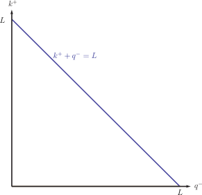
(a) $L<m$

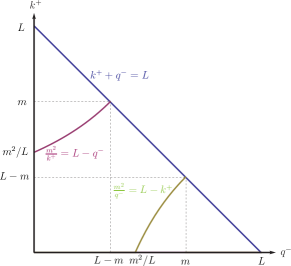
(b) $m<L<(1+\sqrt{5})m/2$

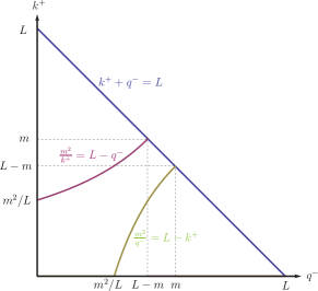
(c) $(1+\sqrt{5})m/2<L<2m$

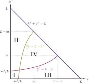
(d) $2m<L$

Figure 9: The integration areas for different parameter regimes. For $L<m$ we have one single integration domain. For $m<L<(1+\sqrt{5})m/2$ and $(1+\sqrt{5})m/2<L<2m$ there are three domains, the regimes differ by the hierarchy between $L-m$ and $m^{2}/L$. Finally, for $L>2m$ we have 4 areas, where the central one (IV) becomes dominating for large values of $L$.

We give a short outline for the calculation of the asymptotic expansion of $\Delta S_{\tau}(\ell,m)$ for large thrust momenta. The asymptotic expansion is performed for each area in Fig. 9d with cutoff regularization taking $m^{2}/L\ll\Lambda_{1}\ll m\ll\Lambda_{2}\ll L$. Area I is suppressed by $m^{6}/L^{6}$ and thus irrelevant. For the computation of the areas II and III we obtain

$$\Delta\mathcal{S}_{\tau}^{(II)}(L,m)=\Delta\mathcal{S}_{\tau}^{(III)}(L,m)=\frac{\alpha_{s}^{2}C_{F}T_{F}}{16\pi^{2}}\left\{\frac{m^{2}}{L^{2}}\right.$$

$$\left.\times\left[2\,\textrm{ln}^{2}\left(\frac{m^{2}}{L^{2}}\right)+12\,\textrm{ln}\left(\frac{m^{2}}{L^{2}}\right)+12+\frac{8\pi^{2}}{3}\right]+\mathcal{O}\left(\frac{m^{3}}{L^{3}}\right)\right\}\,,$$ (94)

The expansions in area IV are cumbersome. We have to go to NLO and consider a large number of different scaling regions with difficult integrations. Special care has to be taken of the power counting for the computation with several cutoffs separating the different regions. Furthermore, cancellations in the denominator appear at NLO which require a special treatment for the hemisphere border region with $q^{-}\approx q^{+}$ and $k^{+}\approx k^{-}$. The calculation for area IV eventually yields

$$\Delta\mathcal{S}_{\tau}^{(IV)}(L,m)=\frac{\alpha_{s}^{2}C_{F}T_{F}}{16\pi^{2}}\left\{-\frac{64}{9}+\frac{104\pi^{2}}{27}-\frac{64\zeta(3)}{3}\right.$$

$$-\frac{m^{2}}{L^{2}}\left[8\,\textrm{ln}^{2}\left(\frac{m^{2}}{L^{2}}\right)+56\,\textrm{ln}\left(\frac{m^{2}}{L^{2}}\right)+\frac{296}{3}+\frac{386\pi^{2}}{45}\right.$$

$$\left.+\left.16\pi\right]+\mathcal{O}\left(\frac{m^{3}}{L^{3}}\right)\right\}\,.$$ (95)

Thus, the final result for the integrated soft function difference reads

$$\Delta\mathcal{S}_{\tau}(L,m)=\frac{\alpha_{s}^{2}C_{F}T_{F}}{16\pi^{2}}\left\{-\frac{64}{9}+\frac{104\pi^{2}}{27}-\frac{64\zeta(3)}{3}\right.$$

$$-\frac{m^{2}}{L^{2}}\left[4\,\textrm{ln}^{2}\left(\frac{m^{2}}{L^{2}}\right)+32\,\textrm{ln}\left(\frac{m^{2}}{L^{2}}\right)+\frac{224}{3}+\frac{146\pi^{2}}{45}\right.$$

$$\left.+\left.16\pi\right]+\mathcal{O}\left(\frac{m^{3}}{L^{3}}\right)\right\}\,,$$ (96)

which gives Eq. (VII).

Appendix B Integral representations of special functions

Here we give explicit integral representations for the Meijer G function $G^{3,0}_{1,3}$ and Struve functions $L_{n}$ ($n<-1/2$) used by Mathematica and appearing in Eqs. (78), (90). For $z>0$ they read

$$G^{3,0}_{1,3}\left(\begin{matrix}1\\ 0,0,0\end{matrix}\middle|\frac{z^{2}}{4}\right)=4\int_{1}^{\infty}\frac{dt}{t}\,K_{0}(zt)\,,$$ (97)

$$L_{n}=I_{-n}(z)-\frac{2^{1-n}z^{n}}{\sqrt{\pi}\,\Gamma\left(n+\frac{1}{2}\right)}\int_{0}^{\infty}dt\left(t^{2}+1\right)^{n-\frac{1}{2}}\sin(tz)\,,$$ (98)

where $K_{n}$ and $I_{n}$ indicate the better known Bessel functions. Computing the integral in Eq. (97) numerically is faster and more stable than evaluating $G^{3,0}_{1,3}$ directly in Mathematica (in particular for large vales of the argument). See also Wolfram for further information about these functions.

References

- (1) S. Weinzierl, NNLO corrections to 3-jet observables in electron-positron annihilation, Phys.Rev.Lett. 101, 162001 (2008).
- (2) S. Weinzierl, Event shapes and jet rates in electron-positron annihilation at NNLO, JHEP 0906, 041 (2009).
- (3) A. Gehrmann-De Ridder, T. Gehrmann, E. Glover, and G. Heinrich, Second-order QCD corrections to the thrust distribution, Phys.Rev.Lett. 99, 132002 (2007).
- (4) A. Gehrmann-De Ridder, T. Gehrmann, E. Glover, and G. Heinrich, NNLO corrections to event shapes in e+ e- annihilation, JHEP 0712, 094 (2007).
- (5) T. Becher and M. D. Schwartz, A Precise determination of from LEP thrust data using effective field theory, JHEP 0807, 034 (2008).
- (6) Y.-T. Chien and M. D. Schwartz, Resummation of heavy jet mass and comparison to LEP data, JHEP 1008, 058 (2010).
- (7) T. Becher and G. Bell, NNLL Resummation for Jet Broadening, JHEP 1211, 126 (2012).
- (8) J.-y. Chiu, A. Jain, D. Neill, and I. Z. Rothstein, The Rapidity Renormalization Group, Phys.Rev.Lett. 108, 151601 (2012).
- (9) J.-Y. Chiu, A. Jain, D. Neill, and I. Z. Rothstein, A Formalism for the Systematic Treatment of Rapidity Logarithms in Quantum Field Theory, JHEP 1205, 084 (2012).
- (10) T. Gehrmann, G. Luisoni, and P. F. Monni, Power corrections in the dispersive model for a determination of the strong coupling constant from the thrust distribution, Eur.Phys.J. C73, 2265 (2013).
- (11) A. H. Hoang and I. W. Stewart, Designing gapped soft functions for jet production, Phys.Lett. B660, 483–493 (2008).
- (12) A. H. Hoang, A. Jain, I. Scimemi, and I. W. Stewart, R-evolution: Improving perturbative QCD, Phys.Rev. D82, 011501 (2010).
- (13) R. Abbate, M. Fickinger, A. H. Hoang, V. Mateu, and I. W. Stewart, Thrust at N3LL with Power Corrections and a Precision Global Fit for , Phys. Rev. D83, 074021 (2011).
- (14) R. Abbate, M. Fickinger, A. H. Hoang, V. Mateu, and I. W. Stewart, Precision Thrust Cumulant Moments at LL, Phys.Rev. D86, 094002 (2012).
- (15) T. Gehrmann, M. Jaquier, and G. Luisoni, Hadronization effects in event shape moments, Eur.Phys.J. C67, 57–72 (2010).
- (16) C. W. Bauer, S. Fleming, and M. E. Luke, Summing Sudakov logarithms in in effective field theory, Phys. Rev. D63, 014006 (2000).
- (17) C. W. Bauer, S. Fleming, D. Pirjol, and I. W. Stewart, An Effective field theory for collinear and soft gluons: Heavy to light decays, Phys. Rev. D63, 114020 (2001).
- (18) S. Fleming, A. H. Hoang, S. Mantry, and I. W. Stewart, Jets from massive unstable particles: Top-mass determination, Phys. Rev. D77, 074010 (2008).
- (19) S. Fleming, A. H. Hoang, S. Mantry, and I. W. Stewart, Top Jets in the Peak Region: Factorization Analysis with NLL Resummation, Phys. Rev. D77, 114003 (2008).
- (20) D. E. Kaplan and M. D. Schwartz, Constraining Light Colored Particles with Event Shapes, Phys.Rev.Lett. 101, 022002 (2008).
- (21) S. Gritschacher, A. H. Hoang, I. Jemos, and P. Pietrulewicz, Secondary Heavy Quark Production in Jets through Mass Modes, Phys.Rev. D88, 034021 (2013).
- (22) R. Kelley, M. D. Schwartz, R. M. Schabinger, and H. X. Zhu, The two-loop hemisphere soft function, Phys. Rev. D84, 045022 (2011).
- (23) A. Hornig, C. Lee, I. W. Stewart, J. R. Walsh, and S. Zuberi, Non-global Structure of the Dijet Soft Function, JHEP 1108, 054 (2011).
- (24) A. H. Hoang and S. Kluth, Hemisphere Soft Function at for Dijet Production in e+ e- Annihilation, arXiv:0806.3852, (2008).
- (25) A. Jain, I. Scimemi, and I. W. Stewart, Two-loop Jet-Function and Jet-Mass for Top Quarks, Phys.Rev. D77, 094008 (2008).
- (26) A. H. Hoang, A. Jain, I. Scimemi, and I. W. Stewart, Infrared Renormalization Group Flow for Heavy Quark Masses, Phys.Rev.Lett. 101, 151602 (2008).
- (27) B. A. Kniehl, M. Krawczyk, J. H. Kuhn, and R. Stuart, Hadronic Contributions to Radiative Corrections in Annihilation, Phys. Lett. B209, 337 (1988).
- (28) A. Hoang, M. Jezabek, J. H. Kuhn, and T. Teubner, Radiation of heavy quarks, Phys.Lett. B338, 330–335 (1994).
- (29) A. Hoang, J. H. Kuhn, and T. Teubner, Radiation of light fermions in heavy fermion production, Nucl. Phys. B452, 173–187 (1995).
- (30) V. A. Smirnov, Asymptotic expansions of two loop Feynman diagrams in the Sudakov limit, Phys.Lett. B404, 101–107 (1997).
- (31) T. Becher and G. Bell, Analytic Regularization in Soft-Collinear Effective Theory, Phys. Lett. B713, 41–46 (2012).
- (32) T. Huber and D. Maitre, HypExp: A Mathematica package for expanding hypergeometric functions around integer-valued parameters, Comput.Phys.Commun. 175, 122–144 (2006).
- (33) T. Hahn, CUBA: A Library for multidimensional numerical integration, Comput.Phys.Commun. 168, 78–95 (2005).
- (34) P. F. Monni, T. Gehrmann, and G. Luisoni, Two-Loop Soft Corrections and Resummation of the Thrust Distribution in the Dijet Region, JHEP 1108, 010 (2011).
- (35) I. W. Stewart, F. J. Tackmann, and W. J. Waalewijn, N-Jettiness: An Inclusive Event Shape to Veto Jets, Phys. Rev. Lett. 105, 092002 (2010).
- (36) M. Beneke, V. M. Braun, and V. I. Zakharov, Bloch-Nordsieck cancellations beyond logarithms in heavy particle decays, Phys.Rev.Lett. 73, 3058–3061 (1994).
- (37) A. Hoang and A. Manohar, Charm effects in the MS-bar bottom quark mass from Upsilon mesons, Phys.Lett. B483, 94–98 (2000).
- (38) A. Hoang, Bottom quark mass from Upsilon mesons: Charm mass effects, arXiv:0008102, (2000).
- (39) S. Gritschacher, A. Hoang, I. Jemos, and P. Pietrulewicz, in preparation.
- (40) Wolfram Research, Inc., The Wolfram Functions Site, 2008-2013, http://functions.wolfram.com.