Resonant radiation shed by dispersive shock waves

Abstract

We show that dispersive shock waves resulting from the nonlinearity overbalancing a weak leading-order dispersion can emit resonant radiation owing to higher-order dispersive contributions. We analyze such phenomenon for the defocusing nonlinear Schrödinger equation, giving criteria for calculating the radiated frequency based on the estimate of the shock velocity, revealing also a diversity of possible scenarios depending on the order and magnitude of the dispersive corrections.

Dispersive shock waves (DSWs) are expanding regions filled with fast oscillations that stem from the dispersive regularization of classical shock waves (SWs). Originally introduced in collisionless plasmas collisionless and water waves water1 , it is only recently that DSWs have been the focus of intense multidisciplinary efforts that have established their universal role in atom condensates BEC ; Hoefer06 , light pulse (temporal) temporal and beam (spatial) spatial propagation, oceanography water , quantum liquids quantum , electron beams electrons , magma flow magma , and granular granular or disordered materials disorder . The dynamics of DSW is understood in terms of weakly dispersive formulation of integrable models (and their defomations) such as the Korteweg De Vries collisionless ; electrons , the Benjamin-Ono quantum ; BO or the defocusing nonlinear Schrödinger equation (dNLSE) Hoefer06 ; temporal ; spatial ; dNLSE . However, since the leading order dispersion of such models must be extremely weak for the phenomenon to take place, one is naturally led to wonder about the effects of higher-order dispersion (HOD). The aim of this Letter is to show that HOD corrections lead DSWs to emit resonant radiation (RR) due to a specific phase-matching with linear waves.
The emission of RR, usually considered for solitons RRoptics ; AK95 ; RRdark ; RRothers ; DudleyRMP06 ; SGRMP10 ; SChydro ; Stark11 ; Joly11 ; Colman12 ; Erkintalo12 , is a relatively well understood phenomenon in connection with studies of supercontinuum generation driven by perturbed solitons of the focusing NLSE (fNLSE) DudleyRMP06 ; SGRMP10 ; SChydro , and the emergence of novel regimes Stark11 ; Joly11 ; Erkintalo12 ; Colman12 ; Bache10 ; rubino12 . Viceversa, the problem of RR from SWs was overlooked. Here we show that perturbed DSWs emit RR, owing to a strong spectral broadening that accompanies wave-breaking and acts as a seed for linear waves that are resonantly amplified thanks to a well defined velocity of the shock front. While we expect this mechanism to be universal for several DSW-bearing models when HOD corrections become effective, we formulate our approach for temporal pulse propagation ruled by the dNLSE spatialHOD , where our results are important in view of generating a different type of supercontinuum pumped in the normal dispersion regime SC12 . They have also immediate impact to unveil the underlying mechanism of recent observations of RR produced by non-soliton pulses Webb13 . We start from the dNLSE in semiclassical form spatial , with dispersion at all orders (sum over $n$ implicitly assumes $n\geq 2$)

$$i\varepsilon\partial_{z}\psi+d(\partial_{t})\psi+|\psi|^{2}\psi=0,$$ (1)

$$d(\partial_{t})\equiv\sum_{n}\frac{\beta_{n}}{n!}\varepsilon^{n}\,(i\partial_{t})^{n}=-\frac{\varepsilon^{2}}{2}\partial^{2}_{t}-i\frac{\beta_{3}\varepsilon^{3}}{6}\partial^{3}_{t}+\frac{\beta_{4}\varepsilon^{4}}{24}\partial^{4}_{t}+\ldots$$

where the link with real-world distance and retarded time (in capital) is $Z=z\sqrt{L_{nl}L_{d}}$, $T=tT_{0}$, where $L_{nl}=(\gamma P)^{-1}$ and $L_{d}=T_{0}^{2}/\partial_{\omega}^{2}k$ are the nonlinear and dispersive length, respectively, associated with input pulse width $T_{0}$ and peak power $P$ ($\gamma$ is the nonlinear coefficient). The dispersive operator $d(\partial_{t})$ have terms which are weighted, without loss of generality, by growing powers of the small parameter $\varepsilon=\sqrt{L_{nl}/L_{d}}\ll 1$ and coefficients $\beta_{n}=\partial_{\omega}^{n}k/\sqrt{(L_{nl})^{n-2}(\partial_{\omega}^{2}k)^{n}}$ (note that $\beta_{2}=1$), $\partial_{\omega}^{n}k$ being $n$-order real-world dispersion arising from usual Taylor expansion of $k(\omega)$ (further details on supplemental material SM ). We assume an input pump $\psi_{0}=\psi(t,z=0)$ with central frequency $\omega_{p}=0$ nota_wp , and denote as $V_{s}$ the “velocity” of the SW produced by $\psi_{0}$ via wave-breaking (here, $V_{s}=dt/dz$ is the reciprocal of the velocity as usually defined for soliton RR AK95 ), and as $\tilde{d}(i\omega)$ the Fourier transform of $d(\partial_{t})$. Linear waves $\exp(ik(\omega)z-i\omega t)$ are resonantly amplified when their wavenumber in the SW moving frame, which reads as $k(\omega)=\frac{1}{\varepsilon}\left[\tilde{d}(i\omega)-V_{s}(\varepsilon\omega)\right]$ equals the pump wavenumber $k_{p}=k(\omega_{p}=0)=0$. Denoting also as $k_{nl}$ the difference between the nonlinear contributions to the pump and RR wavenumber notaRR , respectively, the radiation is resonantly amplified at frequency $\omega=\omega_{RR}$ which solves the equation

$$\sum_{n}\frac{\beta_{n}}{n!}(\varepsilon\omega)^{n}-V_{s}(\varepsilon\omega)=\varepsilon k_{nl}.$$ (2)

At variance with solitons of the fNLSE where $V_{s}(\omega_{p}=0)=0$ AK95 ; SGRMP10 , DSWs possess non-zero velocity $V_{s}$, which must be carefully evaluated, having great impact on the determination of $\omega_{RR}$.

The process of wave-breaking ruled by Eq. (1) can be described by applying the Madelung transformation $\psi=\sqrt{\rho}\exp\left(iS/\varepsilon\right)$. At leading-order in $\varepsilon$, we obtain a quasi-linear hydrodynamic reduction, with $\rho=|\psi|^{2}$ and $u=-S_{t}$ (chirp) equivalent density and velocity of the flow, which can be further cast in the form

$$\partial_{z}\rho+\partial_{t}\left[\sum_{n}\frac{\beta_{n}}{(n-1)!}(\rho u^{n-1})\right]=0,$$ (3)

$$\partial_{z}(\rho u)+\partial_{t}\left[\sum_{n}\frac{\beta_{n}}{(n-1)!}\rho u^{n}+\frac{1}{2}\rho^{2}\right]=0,$$ (4)

of a conservation law $\partial_{z}{\bf q}+\partial_{t}{\bf f}({\bf q})=0$ for mass and momentum, with ${\bf q}=(\rho,\rho u)$. This system can be diagonalized to yield $\partial_{z}r^{\pm}+V^{\pm}\partial_{t}r^{\pm}=0$, by introducing the eigenvelocities $V^{\pm}=\sum_{n}\beta_{n}u^{n-1}/(n-1)!\pm\sqrt{\rho\sum_{n}\beta_{n}u^{n-2}/(n-2)!}$ and the Riemann invariants $r^{\pm}=u\pm 2\frac{\sqrt{\rho}}{\sqrt{\sum_{n}\beta_{n}u^{n-2}/(n-2)!}}$.

Equations (3-4), as far as HOD is such that they remain hyperbolic, admit weak solutions in the form of classical SWs, i.e. traveling discontinuity from left ($\rho_{l},u_{l}$) to right ($\rho_{r},u_{r}$) values, whose velocity $V_{c}$ can be found from the so-called Rankine-Hugoniot (RH) condition $V_{c}({\bf q}_{l}-{\bf q}_{r})=[{\bf f}({\bf q}_{l})-{\bf f}({\bf q}_{r})]$ Whitham74 . In the $2\times 2$ case, the RH equations fix both $V_{c}$ and the admissible value of one of the parameters of the jump, e.g. $u_{r}$ given $\rho_{r},\rho_{l},u_{l}$. For instance, when no HOD is effective (take $\beta_{2}=1$), an admissible right-going shock which satisfies the entropy condition $\rho_{l}>\rho_{r}$, can be obtained with

$$u_{r}=u_{l}-(\rho_{l}-\rho_{r})\sqrt{\frac{\rho_{r}+\rho_{l}}{2\rho_{l}\rho_{r}}};V_{c}=u_{l}+\rho_{r}\sqrt{\frac{\rho_{r}+\rho_{l}}{2\rho_{l}\rho_{r}}}.$$ (5)

This result can be generalized for HOD, thanks to Eqs. (3-4). For instance, if $\beta_{3}\neq 0$, the SW velocity becomes

$$V_{c}=\frac{\beta_{2}(\rho_{l}u_{l}-\rho_{r}u_{r})+\beta_{3}(\rho_{l}u_{l}^{2}-\rho_{r}u_{r}^{2})/2}{(\rho_{l}-\rho_{r})},$$ (6)

where $u_{r}$ is obtained as the real root of the cubic equation $\beta_{3}(u_{l}-u_{r})^{2}(u_{l}+u_{r})+2\beta_{2}(u_{l}-u_{r})^{2}=g(\rho_{l},\rho_{r})$, where $g(\rho_{l},\rho_{r})\equiv(\rho_{l}-\rho_{r})^{2}(\rho_{r}+\rho_{l})/(\rho_{l}\rho_{r})$ (see supplemental for more details SM ).

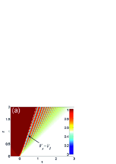
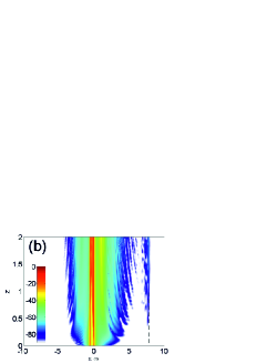
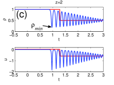
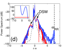
Figure 1: (Color online) Radiating DSW from dNLSE (1) with $\varepsilon=0.03$, input step $\rho_{l},\rho_{r}=1,0.5$, and 3-HOD $\beta_{3}=-0.35$: (a) Color level plot of density $\rho(t,z)$ (the dashed line gives the DSW leading edge velocity $V_{l}$); (b) spectral evolution; (c) snapshots of $\rho,u$ of unperturbed case $\beta_{3}=0$ (in red the corresponding classical SW); (d) output spectra with (blue) and without (red) 3-HOD (input dashed); inset: graphical solution of Eq. (2).

Second-order dispersion, however, is known to regularize classical SWs by replacing the jump with an expanding fan filled with oscillations (i.e. a DSW) characterized by leading $V_{l}$ and trailing $V_{t}$ edge velocities (with $V_{l}<V_{c}<V_{t}$), where the modulated periodic wave locally tends to a soliton and a linear wave, respectively Hoefer06 . HOD induces this structure to radiate, also altering the dynamics of SW formation. Hereafter we specifically focus on the effect of two leading HOD, namely third-order (3-HOD) and fourth-order (4-HOD) dispersion.

In particular, when 3-HOD is effective we find a cross-over from a perturbative regime ($|\beta_{3}|\lesssim 0.5$) where the DSW leading edge turns out to be responsible for the RR, to a regime where the 3-HOD is strong enough ($|\beta_{3}|\sim 1$) to modify the shock formation, leading to enhanced RR produced by a traveling front which is approximated with a classical SW. To show this and verify that Eq. (2) is able to predict the RR frequency in both regimes, we consider first a step initial value that allows us to calculate the velocity analytically, taking $\beta_{3}<0$ without loss of generality. Specifically, we consider the evolution of an initial jump from the state $\rho_{l},u_{l}=0$ to the state $\rho_{r},u_{r}=2(\sqrt{\rho_{r}}-\sqrt{\rho_{l}})$, which is such to maintain constant $r^{-}(z,t)$ upon evolution (only $r^{+}(z,t)$ varies). In this case, the modulated wavetrain produced upon evolution [see Fig. 1(a,c)] in the limit $\beta_{3}=0$ is described by a rarefaction wave of the Whitham modulation equations for the unperturbed dNLSE Hoefer06 . Following the approach of Ref. Hoefer06 , one can calculate the edge velocities of the fan. What is relevant for the RR is the leading-edge velocity, which we find to be $V_{l}=\sqrt{\rho_{l}}+u_{r}=2\sqrt{\rho_{r}}-\sqrt{\rho_{l}}$. Given a gray soliton on unchirped background $A$, $\psi=A[w\tanh(\theta)+iv]\exp(iA^{2}z/\varepsilon)$, $\theta=\frac{w}{\varepsilon}(t-Avz)$, $w^{2}=1-v^{2}$, $V_{l}$ turns out to coincide with the soliton velocity $V_{sol}=Av=\sqrt{\rho_{min}}$, with natural position $A=\sqrt{\rho_{l}}$, $v=(2\sqrt{\rho_{r}}-\sqrt{\rho_{l}})/\sqrt{\rho_{l}}$, and the dip density $\rho_{min}=(2\sqrt{\rho_{r}}-\sqrt{\rho_{l}})^{2}$. We emphasize, however, that the equivalence of the leading edge with a gray soliton holds only locally since the DSW is strictly speaking a modulated nonlinear wave.

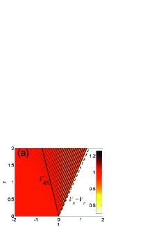
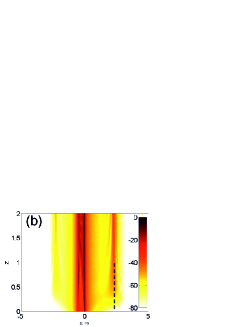
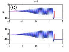
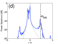
Figure 2: (Color online) As in Fig. 1 with larger 3-HOD $\beta_{3}=-1$. Here $V_{c}=0.69$ and $u_{r}=-0.543$ are the parameters of the classical SW [shown in red in (c)] from Eq. (6). Solid line in (a) indicates the velocity $V_{RR}$ of the RR.

In this regime, if we account for $k_{nl}=k_{nl}^{sol}-k_{nl}^{RR}=-\frac{1}{\varepsilon}\rho_{l}$ arising from the soliton $k_{nl}^{sol}=\rho_{l}/\varepsilon$ and the cross-induced contribution $k_{nl}^{RR}=2\rho_{l}/\varepsilon$ to the RR, Eq. (2) explicitly reads as

$$\frac{\beta_{3}}{6}(\varepsilon\omega)^{3}+\frac{\beta_{2}}{2}(\varepsilon\omega)^{2}-V_{s}(\varepsilon\omega)+\rho_{l}=0.$$ (7)

Real solutions $\omega=\omega_{RR}$ of Eq. (7), with $V_{s}=V_{l}\equiv 2\sqrt{\rho_{r}}-\sqrt{\rho_{l}}$ correctly predicts the RR as long as $|\beta_{3}|\lesssim 0.5$, as shown by the dNLSE simulation in Fig. 1. The DSW displayed in Fig. 1(a) clearly exhibits a spectral RR peak besides spectral shoulders due to the oscillating front, as shown by the spectral evolution in Fig. 1(b) and the output spectrum in Fig. 1(d). Perfect agreement is found between the RR peak obtained in the numerics and the prediction [dashed vertical line in Fig. 1(b,d)] from Eq. (7) with velocity $V_{s}=V_{l}$ characteristic of the integrable limit ($\beta_{3}=0$, snapshots in Fig. 1c). Indeed, in this regime, the DSW leading edge is nearly unaffected by 3-HOD, whereas using the velocity $V_{c}$ [Eq. (5)] of the equivalent classical SW [reported for comparison in Fig. 1(c)] would miss the correct estimate of $\omega_{RR}$. We also point out that $k_{nl}$ represents a small correction, so $\omega_{RR}$ can be safely approximated by dropping the last term in Eq. (7) to yield $\varepsilon\omega_{RR}=\frac{3}{2\beta_{3}}\left(-\beta_{2}\pm\sqrt{\beta_{2}^{2}+8V_{s}\beta_{3}/3}\right)$, or $\varepsilon\omega_{RR}=-\frac{3\beta_{2}}{\beta_{3}}$ for $\beta_{3}V_{s}\rightarrow 0$.

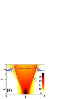
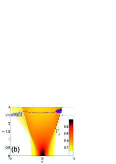
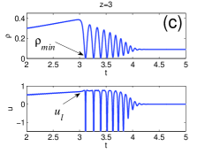
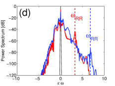
Figure 3: (Color online) Radiating DSW from Gaussian pulses with small background $\nu^{2}=0.09$: (a) $\beta_{3}=-0.35$; (b) $\beta_{3}=-0.6$; (c) Parameters determining the leading edge velocity $V_{s}=\sqrt{\rho_{min}}+u_{l}=\sqrt{10^{-4}}+0.76=0.77$ [dashed line in (a)]; (d) Output spectra (blue, $\beta_{3}=-0.35$; red, $\beta_{3}=-0.6$). The dashed lines give $\varepsilon\omega_{RR}$ calculated from Eq. (7). Here $\varepsilon=0.03$; blue curves in (a),(b) depict output shapshots.

When $|\beta_{3}|$ grows larger, the aperture of the shock fan reduces, until eventually the DSW resembles a single traveling front, i.e. a classical SW El . In this regime, we find that Eq. (7) still gives the correct frequency $\omega_{RR}$ provided that $V_{s}$ is taken as the Rankine-Hugoniot velocity $V_{c}$ of the equivalent classical SW calculated for $\beta_{3}\neq 0$ [Eq. (6)]. This case is illustrated in Fig. 2 for $\beta_{3}=-1$. The RR becomes clearly visible in the temporal evolution [Fig. 2(a,c)], and is sufficiently strong to generate $-\omega_{RR}$ via four-wave mixing [Fig. 2(b-d)]. Perfect agreement between the numerics and the value predicted from Eq. (7), once we set $V_{s}=V_{c}$, is found also in this case.

The behaviors of step initial data are basically recovered for pulse waveforms that are more manageable in experiments. Figure 3 shows the transition from the perturbative [Fig. 3(a)] to the non-perturbative [Fig. 3(b)] regime, for an input gaussian pulse $\psi_{0}=\nu+(1-\nu)\exp(-t^{2})$ with background to peak density ratio $\nu^{2}=0.09$. As shown in Fig. 3(a), for relatively small $\beta_{3}$, two asymmetric DSWs emerge from wave-breaking points on the two pulse edges, which occur at different distances due to broken symmetry in time caused by 3-HOD. Phase-matching is achieved only for the DSW traveling with $V_{s}>0$. The corresponding $\omega_{RR}$ can be obtained from Eq. (7) provided we set $V_{s}=V_{l}$, with the DSW leading edge velocity being (following the discussion of Fig. 1) $V_{l}=\sqrt{\rho_{min}}+u_{l}$, where the minimum density and the correction $u_{l}$ due to the local non-zero chirp are evaluated numerically after wave-breaking as shown in Fig. 3(c). Also in this case, a larger $|\beta_{3}|$ results in a narrower fan, until eventually a simple front is left which strongly radiates, as shown in Fig. 3(b). In this regime, a good approximation of the front velocity is obtained by the approximating classical SW in Eq. (6). In both the regimes shown in Fig. 3(a) and (b), Eq. (7) provides a good description of the RR frequency observed in the numerics [see Fig. 3(d)]. Notice also that, for symmetry reasons, sign reversal of 3-HOD (i.e., $\beta_{3}>0$) simply results into RR with opposite frequency, generated by the DSW with opposite velocity ($V_{s}<0$, left DSW).

We also emphasize two important points: (i) RR occurs also in the limit of vanishing background $\nu=0$, as shown in Fig. 4(a), allowing us to conclude that a bright pulse does not need to be a soliton (as in the fNLSE, $\beta_{2}=-1$) to radiate. Importantly, experimental evidence for such RR scenario was reported very recently in fiber optics Webb13 , without explaining the underlying mechanism, which our theory individuates in the shock formation. Indeed, the physical parameters used in Fig. 1 of Ref. Webb13 , i.e. power $P=600$ W, pulse duration $T_{0}=1$ ps, nonlinear coefficient $\gamma=2.5$ W^-1 km^-1, dispersion $\partial^{2}_{\omega}k=7.5$ ps²/km, $\partial^{3}_{\omega}k=0.2$ ps³/km, gives normalized parameters $\varepsilon\simeq 0.07$ and $\beta_{3}\simeq 0.37$, typical of the wave-breaking regime ($\varepsilon\ll 1$) with perturbative 3-HOD. Since $\beta_{3}>0$, the radiating shock turns out to be the one on the leading edge ($t<0$), and its velocity $V_{s}=-0.75$, inserted in Eq. (2), gives a negative [opposite of Fig. 4(a)] frequency detuning $\Delta f_{RR}=\omega_{RR}T_{0}^{-1}/2\pi\simeq 13$ THz, in excellent agreement with the value reported in Ref. Webb13 . (ii) a limitation exists (regardless of $\nu$) on the value of $|\beta_{3}|$ to observe RR, since large 3-HOD feature a qualitative different wave-breaking mechanism, as shown in Fig. 4(b) for $\beta_{3}=-2$. While the non-radiating (left) DSW simply develop at shorter $z$ without qualitative changes, on the right ($t>0$) the pulse undergoes a different catastrophe, reminiscent of the fNLSE. Indeed in this case the eigenvelocities $V^{\pm}=\beta_{2}u+\beta_{3}u^{2}/2\pm\sqrt{\rho(\beta_{2}+\beta_{3}u)}$ become locally complex conjugate where $u>0$, implying that Eqs. (3-4) show a mixed hyperbolic-elliptic behavior reminiscent of the so-called transsonic flow transsonic .

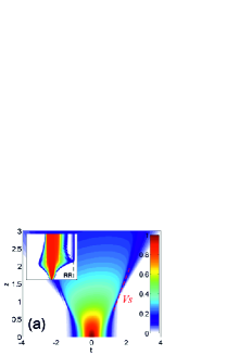
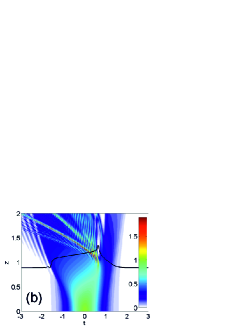
Figure 4: (Color online) (a) Temporal evolution of a Gaussian pulse without background, for $\beta_{3}=-0.35$. Inset shows spectral evolution. (b) Mixed hyperbolic-elliptic type of wave-breaking for large 3-HOD $\beta_{3}=-2$, $\nu^{2}=0.01$. Solid line, snapshot at $z=0.9$. Here $\varepsilon=0.03$.

A completely different scenario occurs when the dispersive correction is due to 4-HOD. In this case, the shock formation can compete with a different breaking mechanism, namely modulational instability (MI). The latter, characteristic of the fNLSE, is known to extend to the defocusing regime $\beta_{2}=1$, whenever $\beta_{4}<0$ MI (see also supplemental material SM ). Moreover, the problem is symmetric in time and the shocks from both edges of a pulse radiate. Overall four RR frequencies result from Eq. (2), which is now fourth-order: the frequency pair $\omega_{RR1},-\omega_{RR2}$ ($\omega_{RR1,RR2}>0$) and the opposite pair $-\omega_{RR1},\omega_{RR2}$, induced by the shock with positive ($V_{s}>0$) and negative velocity ($V_{s}>0$), respectively. Since the MI has a spectral narrow bandwidth that turns out to lie exactly in between the two frequencies $\omega_{RR1,RR2}$ (arising from shocks on opposite edges), it serves as a seed for the RR. This is shown in Fig. 5: the pair of twin-band RR starts to grow, triggered by MI, even during the process of pulse edge steepening ($z<1$), while becoming prominent as the DSWs form and travel with definite velocities (here $V_{s}=\pm 0.77$). The four-band RR from the spectral evolution in Fig. 5(b) fits well the prediction from Eq. (2) (dashed lines), while coexistence of the two wave-breaking phenomena (MI and DSW) is clearly visible in the output snapshot in Fig. 5(a).

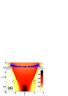
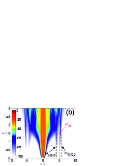
Figure 5: (Color online) RR ruled by 4-HOD ($\beta_{3}=0$, $\beta_{4}=-0.5$): (a) temporal dynamics (blue curve depicts output snapshot); (b) spectral evolution, black dashed lines are prediction from Eq. (2), red dashed line is MI peak gain. Here $\varepsilon=0.05$, input Gaussian pulse with background $\nu^{2}=0.09$.

In summary, we have demonstrated that higher-order dispersive corrections force DSWs to radiate, following different observable cross-over scenarios depending on the nature and magnitude of such corrections.
Funding from MIUR (grant PRIN 2009P3K72Z) is gratefully acknowledged.

References

- (1) R. Z. Sagdeev, Sov. Phys. Tech. Phys. 6, 867 (1962); R.J. Taylor, D.R. Baker, and H. Ikezi, Phys. Rev. Lett. 24, 206 (1970); A.V. Gurevich and L.P. Pitaevskii, Sov. Phys. JETP 38, 291 (1974);
- (2) T.B. Benjamin and M.J. Lighthill, Proc. Roy. Soc. Lond. A, 224, 448 (1954); D. H. Peregrine, J. Fluid Mech. 25, 321 (1966).
- (3) Z. Dutton et al., Science 293, 663 (2001); A.M. Kamchatnov, A. Gammal, and R.A. Kraenkel, Phys. Rev. A 69, 063605 (2004); R. Meppelink et al., Phys. Rev. A80, 043606 (2009).
- (4) M. A. Hoefer, M. J. Ablowitz, I. Coddington, E. A. Cornell, P. Engels, and V. Schweikhard, Phys. Rev. A74, 023623 (2006); J.J. Chang, P. Engels, and M.A. Hoefer, Phys. Rev. Lett. 101, 170404 (2008).
- (5) J. E. Rothenberg and D. Grischkowsky, Phys. Rev. Lett. 62, 531 (1989); Y. Kodama, S. Wabnitz, and K. Tanaka, Opt. Lett. 21, 719 (1996); C. Conti, S. Stark, P. St. J. Russell, and F. Biancalana, Phys. Rev. A 82, 013838 (2010); M. Conforti, F. Baronio, and S. Trillo, Opt. Lett. 37, 1082 (2012); J. Fatome et al., Observation of colliding optical undular bores spontaneously generated via four-wave mixing in optical fibres, submitted to Nature Photonics.
- (6) W. Wan, S. Jia, and J. W. Fleischer, Nature Phys. 3, 46 (2007); Phys. Rev. Lett. 99, 223901 (2007); N. Ghofraniha, C. Conti, G. Ruocco, and S. Trillo, Phys. Rev. Lett. 99, 043903 (2007); C. Conti et al., Phys. Rev. Lett. 102, 083902 (2009).
- (7) N.F. Smyth, P.E. Holloway, J. Phys. Oceanogr. 18, 947(1988); G. A. El, H. J. Grimshaw, A. M. Kamchatnov, Stud. Appl. Math. 114, 395 (2005); J. R. Apel, J. Phys. Oceanogr. 33, 2247 (2003).
- (8) E. Bettelheim, A.G. Abanov, P. Wiegmann, Phys. Rev. Lett. 97, 246401 (2006).
- (9) Y. C. Mo et al., Phys. Rev. Lett. 110, 084802 (2013).
- (10) N. K. Lowman and M. A. Hoefer, J. Fluid Mech. 718, 524 (2013).
- (11) P. Lorenzoni and S. Paleari, Phys. D 221, 110 (2006); A. Molinari and C. Daraio, Phys. Rev. E 80, 056602 (2009).
- (12) N. Ghofraniha, S. Gentilini, V. Folli, E. Del Re, and C. Conti, Phys. Rev. Lett. 109, 243902 (2012).
- (13) P. D. Miller and Z. Xu, Commun. Pure Appl. Math. 64, 205 (2010).
- (14) A.V. Gurevich and A. L. Krylov, Sov. Phys. JETP 65, 944 (1987); A.V. Gurevich, A. L. Krylov, and G.A. El, Sov. Phys. JETP 74, 957 (1992).
- (15) P. K. A. Wai, C. R. Menyuk, Y. C. Lee, and H. H. Chen, Opt. Lett. 11, 464 (1986); ibidem, 12, 628 (1987); P. K. A. Wai, H. H. Chen, and Y. C. Lee, Phys. Rev. A 41, 426 (1990).
- (16) N. Akhmediev and M. Karlsson, Phys. Rev. A 51, 2602 (1995).
- (17) H. H. Kuehl and C. Y. Zhang, Phys. Fluids B 2, 889 (1990); V. I. Karpman and H. Schamel, Phys. Plasmas 4, 120 (1997); V. I. Karpman, Phys. Rev. E 58, 5070 (1998).
- (18) V. V. Afanasjev and Y. S. Kivshar, and C. R. Menyuk, Opt. Lett. 21, 1975 (1996); C. Milian, D. V. Skryabin, and A. Ferrando, Opt. Lett. 34, 2096 (2009).
- (19) D. V. Skryabin and A. V. Gorbach, Rev. Mod. Phys. 82, 1287 (2010).
- (20) J. M. Dudley, G. Genty, and S. Coen, Rev. Mod. Phys. 78, 1135 (2006).
- (21) A. Chabchoub, N. Hoffmann, M. Onorato, G. Genty, J. M. Dudley, and N. Akhmediev, Phys. Rev. Lett. 111, 054104 (2013).
- (22) S. P. Stark, A. Podlipensky, and P. St. J. Russell, Phys. Rev. Lett. 106, 083903 (2011).
- (23) N.Y. Joly, J. Nold, W. Chang, P. Hölzer, A. Nazarkin, G. K. L. Wong, F. Biancalana, and P. St. J. Russell, Phys. Rev. Lett. 106, 203901 (2011); M. F. Saleh et al., Phys. Rev. Lett. 107, 203902 (2011).
- (24) M. Erkintalo, Y.Q. Xu, S.G. Murdoch, J.M. Dudley, and G. Genty, Phys. Rev. Lett. 109, 223904 (2012).
- (25) P. Colman et al., Phys. Rev. Lett. 109, 093901 (2012).
- (26) B. B. Zhou, A. Chong, F. W. Wise, and M. Bache, Phys. Rev. Lett. 19, 18754 (2012); M. Conforti and F. Baronio, J. Opt. Soc. Am. B 30, 1041 (2013).
- (27) E. Rubino, J. McLenaghan, S. C. Kehr, F. Belgiorno, D. Townsend, S. Rohr, C. E. Kuklevicz, U. Leonhardt, F. König, and D. Faccio, Phys. Rev. Lett. 108, 253901 (2012).
- (28) HOD-terms are relevant also for spatial problems to account for non-paraxial effects, see e.g. C. Conti, G. Ruocco, and S. Trillo, Phys. Rev. Lett. 95, 183902 (2005).
- (29) Y. Liu, H. Tu, and S. A. Boppart Opt. Lett. 37, 2172 (2012)
- (30) K. E. Webb, Y. Q. Xu, M. Erkintalo, and S. G. Murdoch, Opt. Lett. 38, 151 (2013).
- (31) See Supplemental Material at [URL will be inserted by publisher] for more technical details on the normalization of Eq. (1), evaluation of Rankine-Hugoniot velocity, and MI analysis in the presence of 4-HOD.
- (32) This simply means, without loss of generality, that in real world units coincides with , around which in Eq. (1) is expanded
- (33) The nonlinear contribution to the wawenumber of the resonant radiation is induced by cross-phase modulation with a non-zero background, on top of which RR propagates.
- (34) G. B. Whitham, Linear and Nonlinear Waves (Wiley, New York, 1974).
- (35) in the intermediate regime , an estimate of the leading edge velocity could be given via a non-integrable formulation of the Whitham modulation theory, see G. A. El, Chaos 15, 1 (2005) and Ref. [10], which we will develop elsewhere.
- (36) J.C. Di Franco, P. D. Miller, and B. K. Muite, Acta Math. Scientia 31B, 2343 (2011).
- (37) S. B. Cavalcanti, J. C. Cressoni, H. R. da Cruz, and A. S. Gouveia-Neto, Phys. Rev. A43, 6162 (1991); S. Pitois and G. Millot, Opt. Commun. 226 415 (2003); J. D. Harvey, R. Leonhardt, S. Coen, G. K. L. Wong, J. C. Knight, W. J. Wadsworth, and P. S. J. Russell, Opt. Lett. 28, 2225 (2003).