Finite temperature dynamics of vortices in Bose-Einstein condensates

Abstract

We study the dynamics of a single and a pair of vortices in quasi two-dimensional Bose-Einstein condensates at finite temperatures. We use the stochastic Gross-Pitaevskii equation, which is the Langevin equation for the Bose-Einstein condensate, to this end. For a pair of vortices, we study the dynamics of both the vortex-vortex and vortex-antivortex pairs, which are generated by rotating the trap and moving the Gaussian obstacle potential, respectively. Due to thermal fluctuations, the constituent vortices are not symmetrically generated with respect to each other at finite temperatures. This initial asymmetry coupled with the presence of random thermal fluctuations in the system can lead to different decay rates for the component vortices of the pair, especially in the case of two corotating vortices.

I Introduction

In the spin zero or scalar Bose-Einstein condensates (BECs), vortices carry integral angular momentum and serve as the unambiguous proof of superfluidity of these systems. The various methods which have been employed by the experimentalists to generate the vortices in BECs include manipulating the interconversion between the internal spin states of an isotope Matthews , stirring the BEC with the laser beam Madison ; Raman , rotating the BEC Abo-Shaeer , phase imprinting Leanhardt , etc. Vortex dipoles, consisting of vortex-antivortex pairs, have also been experimentally realized in BECs by moving the condensate across the Gaussian obstacle potential Neely . Vortex dipoles are also formed as the decay product of the soliton in quasi two-dimensional condensates Anderson . More recently, formation of the vortex dipoles during the rapid quench through the condensation temperature has also been observed Weiler ; Freilich The dynamics of a single vortex and a vortex-antivortex pair has also been observed experimentally Freilich . On theoretical front, the dynamics of vortex dipoles has also been analyzed at zero temperature Middelkamp ; Torres . Recently, the dynamics of small vortex clusters with $2$-$4$ corotating vortices was also studied both experimentally and theoretically Navarro . The decay of an off-centered vortex at finite temperature has been studied using pure classical field treatment Schmidt , dissipative Gross-Pitaevskii equation (DGPE) Madarassy , Zaremba-Nikuni-Griffin (ZNG) formalism Jackson ; Allen , projected Gross-Pitaevskii equation (PGPE) Wright , and stochastic projected Gross-Pitaevskii equation (SPGPE) Rooney .

To the best of our knowledge, the finite temperature dynamics of a pair of vortices has not been investigated theoretically which we do in the present work, along with a study of the dynamics of a single vortex. The method we employ is the stochastic Gross-Pitaevskii equation (SGPE) Stoof-1 ; Duine-1 ; Stoof-2 . For the case of a single vortex in a condensate with Thomas-Fermi density profile, the present work is the first one to employ the SGPE, which is a better method than ZNG in low-dimensional systems near critical temperatures. In weakly interacting domain, where the condensate has the Gaussian density profile, the stochastic equations of motion for the position of vortex core have also been derived using a variational approach to the SGPE Duine-2 . The SGPE has been successfully used to study finite temperature scalar BECs in quasi one- and two-dimensional geometries Proukakis-1 ; Cockburn-1 ; Cockburn-2 ; Cockburn-3 ; Cockburn-4 ; Cockburn-5 .

The paper is organized as follows: In Sec. II, we describe the SGPE method. We then discuss the finite temperature dynamics of a single vortex in Sec. III. This is followed by the investigation of the dynamics of a vortex pair in Sec. IV. We conclude by providing the summary and conclusions in the last section.

II Stochastic Langevin equation for the BEC

At $T=0~{}$K, a scalar BEC is well described by the Gross-Pitaevskii (GP) equation Dalfovo

$$i\hbar\frac{\partial\Phi(\mathbf{x},t)}{\partial t}=\left(-\frac{\hbar^{2}\nabla^{2}}{2m}+V(\mathbf{x})+g|\Phi(\mathbf{x},t)|^{2}\right)\Phi(\mathbf{x},t),$$ (1)

where $\Phi(\mathbf{x},t)$ is the wave function of the BEC. The trapping potential $V(\mathbf{x})=(\omega_{x}^{2}x^{2}+\omega_{y}^{2}y^{2}+\omega_{z}^{2}z^{2})/(2m)$. The interaction between atoms with mass $m$ is characterized by the interaction strength $g=4\pi\hbar^{2}a/m$, where $a$ is the $s$-wave scattering length. The GP equation conserves the total number of atoms and total energy. In order to study the finite temperature scalar BEC, we use the stochastic Gross-Pitaevskii equations (SGPE) Cockburn-1

$$i\hbar\frac{\partial\Psi(\mathbf{x},t)}{\partial t} = (1-i\gamma)\left(-\frac{\hbar^{2}\nabla^{2}}{2m}+V+g|\Psi(\mathbf{x},t)|^{2}-\mu\right)$$ (2)

$$\Psi(\mathbf{x},t)+\eta(\mathbf{x},t),$$

where $\gamma$ is the dissipation, $\mu$ is the chemical potential, and $\eta(\mathbf{x},t)$ is the random fluctuation which satisfies the following noise-noise correlation

$$\langle\eta(\mathbf{x},t)\eta^{*}(\mathbf{x}^{\prime},t^{\prime})\rangle=2\gamma k_{B}T\hbar\delta(\mathbf{x-x^{\prime}})\delta(\mathbf{t-t^{\prime}}),$$ (3)

according to the fluctuation-dissipation theorem required for equilibration, where $k_{B}$ and $T$ are the Boltzmann constant and temperature respectively, and $\langle\ldots\rangle$ denotes the averaging over different noise realizations. The system described by the SGPE is assumed to be divided into two parts: The first consisting of a few highly occupied low lying modes is represented by a Langevin field $\Psi(\mathbf{x},t)$ and the second, representing a heat bath, is denoted by the noise $\eta$. The effect of the higher modes is taken into account by the noise. The Langevin field is the expectation value of the annihilation field operator $\hat{\Psi}$ at zero temperature and at finite temperature has contributions from thermal fluctuations, i.e.,

$$\Psi=\langle\hat{\Psi}\rangle+\delta\hat{\Psi}\equiv\Phi+\delta\hat{\Psi},$$ (4)

where $\Phi$ is the solution of Eq. (1). While numerically solving the SGPE, the division into the low lying modes represented by the Langevin field and all the higher modes represented by the noise is automatically implemented by numerical discretisation. The discretisation introduces the ultraviolet momentum cutoff, which separates the multimode Langevin field from the higher modes. An important assumption that is made while deriving the SGPE equation is that the thermal atoms are assumed to have a Rayleigh-Jeans distribution with non-zero chemical potential instead of a Bose-Einstein distribution. Due to this assumption, the dynamics obtained from the SGPE is sensitive to the ultraviolet energy cutoff imposed on the system. In the numerical simulations, the energy cutoff and the finite grid spacing are related by

$$E_{\rm cutoff}=\frac{\hbar^{2}|\mathbf{k}_{\rm cutoff}|^{2}}{2m}=\frac{\pi k_{B}T}{2}\left(\frac{\lambda_{T}}{\alpha}\right)^{2},$$ (5)

where $\alpha$ is the grid spacing in the square lattice and $\lambda_{T}$ is the thermal de Broglie wavelength. In the present work, we consider $\delta x=\delta y=\alpha=0.11$, where $\delta x$ and $\delta y$ are the grid spacings along the $x$ and $y$ directions respectively. Before proceeding further, we transform the SGPE into dimensionless form using following transformations:

$$\mathbf{x} = \tilde{\mathbf{x}}a_{\rm osc},~{}t=\frac{2\tilde{t}\omega^{-1}}{1+\gamma^{2}},~{}\Psi=\frac{\tilde{\Psi}}{a_{\rm osc}^{3/2}},~{}\eta=\frac{\hbar\omega}{a_{\rm osc}^{3/2}}\tilde{\eta}$$ (6)

where $a_{\rm osc}=\sqrt{\hbar/(m\omega)}$ with $\omega=\rm min~{}\{\omega_{x},\omega_{y},\omega_{z}\}$ is the oscillator length. The dimensionless SGPE equation for the BEC is now of the form

$$(i-\gamma)\frac{\partial\tilde{\Psi}}{\partial\tilde{t}} = \left(-\tilde{\nabla}^{2}+2\tilde{V}+2\tilde{g}|\tilde{\Psi}|^{2}-2\tilde{\mu}\right)\tilde{\Psi}$$ (7)

$$+2\frac{\tilde{\eta}(\tilde{\mathbf{x}},\tilde{t})}{1-i\gamma},$$

where $\tilde{V}=(\lambda_{x}^{2}\tilde{x}^{2}+\lambda_{y}^{2}\tilde{y}^{2}+\lambda_{z}^{2}\tilde{z}^{2})/2$. Also, $\lambda_{\alpha}=\omega_{\alpha}/\omega$ with $\alpha=x,y,z$ and $\tilde{g}=4\pi\hbar Na/(3m\omega a_{\rm osc}^{3})$. The noise-noise correlation in scaled coordinates now reads

$$\langle\tilde{\eta}(\tilde{\mathbf{x}},\tilde{t})\tilde{\eta}^{*}(\tilde{\mathbf{x}}^{\prime},\tilde{t}^{\prime})\rangle=\gamma\frac{k_{B}T}{\hbar\omega}(1+\gamma^{2})\delta(\tilde{\mathbf{x}}-\tilde{\mathbf{x}}^{\prime})\delta(\tilde{t}-\tilde{t}^{\prime}).$$ (8)

For the sake of simplicity of notations, from here on we will show the scaled variables without tildes in the rest of the manuscript except if mentioned otherwise. In the present work, we consider the BEC in quasi two-dimensional traps for which $\lambda_{x}=\lambda_{y}=1\ll\lambda_{z}$. In this case, the axial degrees of freedom of the system are frozen. We write $\Psi(\mathbf{x})=\zeta(z)\psi(x,y)$ with $\zeta(z)=(\lambda_{z}/\pi)^{1/4}e^{-(\lambda_{z}z^{2})/2}$ as the harmonic oscillator ground state along the axial direction. This allows us to use the following two-dimensional equation after integrating out the axial coordinate:

$$(i-\gamma)\frac{\partial\psi}{\partial t} = \left(-\nabla_{xy}^{2}+2V_{xy}+2g_{xy}|\psi|^{2}-2\mu\right)\psi$$ (9)

$$+\frac{2\eta}{1-i\gamma},$$

where $\nabla_{xy}^{2}=\partial^{2}/\partial x^{2}+\partial^{2}/\partial y^{2}$, $V_{xy}=x^{2}/2+y^{2}/2$ and $g_{xy}=\sqrt{\lambda_{z}/2\pi}g$. We use time splitting Fourier spectral method to solve equation Eq. (9) on $256\times 256$ square grid Bao . The spatial and time step sizes employed in the present work are $0.11$ and $0.006$ respectively.

In the SGPE, physical properties are calculated by averaging over several independent noise realizations. Thus, it has a close resemblance to experiments, where relevant data is obtained by averaging over several independent experimental realizations. In other words, the individual results obtained with independent noise realizations are equivalent to the individual results obtained from independent experimental realizations. Due to the random nature of the noise, the results of various noise realizations will differ from one another as is the case in experiments. Herein lies the first advantage of SGPE method as it can account for experimental shot to shot variation in the properties of the system, whereas methods like the ZNG can very accurately account only for the average properties. The second advantage is that in contrast to the ZNG formalism, the SGPE method can also fully describe the regimes where the thermal fluctuations in the condensate phase are quite large, e.g. one- and two-dimensional systems at temperatures close to the transition temperature. Among the other methods used to study finite temperature BECs, the stochastic projected Gross-Pitaevskii equation (SPGPE) has a resemblance to the SGPE Blakie ; Gardiner-1 ; Gardiner-2 . The crucial difference is the use of projector to extract the low lying coherent modes in SPGPE.

The SGPE simulates the system in a grand canonical ensemble since there is no conservation of the atom number. The equilibrium value of the number of atoms is fixed by the chemical potential. While studying the dynamics, especially in the presence of strong perturbations the fluctuations in atom number above the mean may be quite large. However, at very low temperatures or over small time scales after the system has reached equilibrium, the atom number may be approximately conserved. This situation can be mimicked by first generating the equilibrium solution using the SGPE and then switching of the dissipation and noise, i.e., setting $\gamma=\eta=0$ to study the dynamics. This method ensures atom number conservation over the regime of interest and is denoted as SGPE_eq in this paper. This method has been earlier used to model the quasi condensate growth on an atom chip Proukakis-2 and is similar in spirit, to the truncated Wigner method Steel .

III Dynamics of a single vortex

We first study the dynamics of a single vortex, which is created in the BEC by rotating it at an optimum frequency, at finite temperature. In the present work, we consider $\approx 1\times 10^{5}$-$1.5\times 10^{5}$ atoms of ⁸⁷Rb trapped in a trapping potential with $\omega=\omega_{x}=\omega_{y}=2\pi\times 10$ Hz and $\omega_{z}=2\pi\times 100$ Hz. With this choice of parameters, $a_{\rm osc}=3.41~{}\mu$m and $\omega^{-1}=1.59\times 10^{-2}$s, the respective units of length and time employed in the manuscript. The $s$-wave scattering length of ⁸⁷Rb is $99a_{0}$. Let us term this set of parameters as parameters set a. The critical temperature obtained by using the expression for an ideal three-dimensional Bose gas $T^{3d}_{c}=\hbar\bar{\omega}N^{1/3}/k_{B}$ is $\approx 45-52~{}{\rm nK},$ where $\bar{\omega}=(\omega_{x}\omega_{y}\omega_{z})^{1/3}$. The expression is valid provided $k_{B}T\gg\hbar\omega$. On the other hand, the transition temperature for a strictly two-dimensional ideal Bose gas is $T^{2d}_{c}=\sqrt{6N\omega_{x}\omega_{y}}\hbar/\pi k_{B}\approx 118-145~{}{\rm nK}.$ Bagnato In the quasi two-dimensional case with finite $\tilde{\omega}_{z}=\hbar\omega_{z}/k_{B}T^{2d}_{c}$, the critical temperature is significantly reduced Holzmann , and for the aforementioned parameters $T^{q2d}_{c}=0.37T^{2d}_{c}\approx 44-53~{}{\rm nK}$, and hence is closer to the value for a three dimensional ideal Bose gas. In the present work, we study the dynamics of vortices in BECs at finite temperatures, which can be as high as $50$ nK, where thermal fluctuations are appreciable.

The dissipation parameter $\gamma$ is in general a function of both space and time, but in the present work we consider it to be independent of spatial and temporal coordinates. An approximate damping based on microscopic considerations has been suggested by Penckwitt et al. Penckwitt which gives us the damping parameter

$$\gamma=\kappa\frac{4mk_{B}T}{\pi}\left(\frac{a}{\hbar}\right)^{2},$$ (10)

where $\kappa=3$. This choice of $\kappa=3$ reproduces the growth rate observed in most experiments Penckwitt .

We first generate a single vortex by rotating the condensate with a frequency $\Omega=0.1~{}\omega_{x}$ at $T=30$ nK, $40$ nK and $50$ nK. Having generated a vortex, we switch off the rotation. The density and phase profiles of the condensate just prior to switching off the rotation can be seen in the upper panel of Fig. 1 for a temperature of $40$ nK.

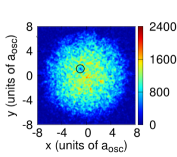
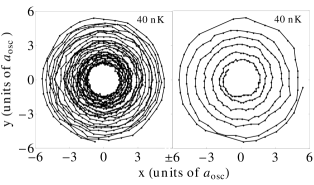
Figure 1: (Color online) The upper panel shows the density (left image) and phase profile (right image) of the condensate just before switching off the rotational frequency at $T=40$ nK. The location of the vortex has been marked by a black circle in both the density and phase profiles. The lower panel shows the trajectory traversed by the vortex for two different values of $\gamma$; $\gamma=7.5\times 10^{-4}$ (left) and $\gamma=7.5\times 10^{-3}$ (right).

In steady state, the position of the vortex is different at different temperatures. We let the system evolve after switching off the rotation and observe that with the passage of time the vortex slowly spirals out of the condensate for all the aforementioned temperatures. This leads to the decrease in the energy of the system. As an example, the trajectories traversed by the vortex at $40$ nK for two different values of $\gamma$, $\gamma=7.5\times 10^{-4}$ obtained from Eq. (10) and $\gamma=7.5\times 10^{-3}$, are shown in the lower panel of Fig. 1. In both the cases, the vortex slowly spirals out of the condensate with a greater rate of decay for a larger value of $\gamma$. The exact dynamics of the off-center vortex at $T=30$ nK, $40$ nK and $50$ nK temperatures is shown in Fig. 2.

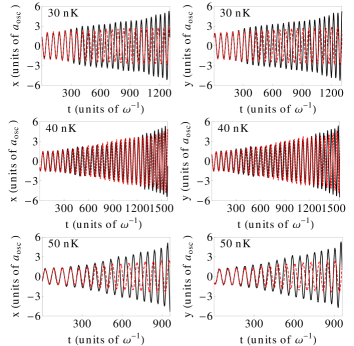
Figure 2: (Color online) Dynamics of a single off-center vortex at $30$ nK (upper panel), $40$ nK (middle panel) and $50$ nK (lower panel). The plots on the left show the $x$-coordinate of the vortex as a function of time, while the plots on the right show the $y$-coordinate of the vortex as a function of time. Solid-black and dashed-red curves correspond to results obtained using SGPE and SGPE_eq respectively.

We find that the results of number conserving SGPE_eq agree with those of the SGPE for the initial period of evolution. This is evident from the dynamics in Fig. 2 up to $t=300~{}\omega^{-1}$. Within this period, the agreement between the SGPE_eq and the SGPE dynamics is better at lower temperatures. It implies that the effect of the noise, which accounts for modes with energy higher than $E_{\rm cutoff}$, is negligible over small time scales. Over this period, the multimode Langevin field solely describes the system dynamics. The SGPE_eq results in much slower decay of the vortex as compared to SGPE as is evidenced by the lower amplitude of oscillations of the $x$- and $y$-coordinates of the vortex in Fig. 2. We find that the decay rate of the vortex depends on its initial location as well as temperature. In our simulations, the vortex created at $40$ nK takes a much longer time to decay than the vortex created at $30$ nK as is shown in Fig 2. At $40$ nK the vortex, just prior to switching off the rotation, is located closer to trap center as compared to its location at $30$ nK. Hence, the density of the thermal atoms is lower in the vicinity of the vortex at $40$ nK than at the $30$ nK. This leads to the slower decay rate at $40$ nK temperature. These results are in qualitative agreement with previous studies Jackson ; Allen ; Rooney . In the present work, as we cannot precisely control the initial location of the vortex, quantitative comparison with earlier studies is not possible. The actual variation in the number of atoms within the SGPE after the rotation is switched off is shown in Fig. 3.

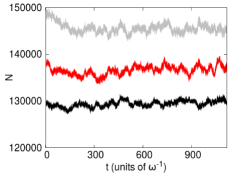
Figure 3: (Color online) The plot shows the number of atoms as function of time, obtained using SGPE, after switching off the $\Omega$. The black, red and grey curves correspond to $30$ nk, $40$ nK, and $50$ nK temperatures respectively. In SGPE_eq, the number remains fixed to the value at $t=0$ at all temperatures.

IV Dynamics of a vortex pair

IV.1 Dynamics of two corotating vortices

Extending the method discussed in the previous section, we can also study the dynamics of a corotating vortex pair at a finite temperature near the condensation temperature. We first generate a vortex pair by rotating the condensate at finite temperature with a frequency $\Omega=0.16~{}\omega_{x}$. The density and phase profiles of the condensate before switching off the rotational frequency at $30$ nK and $40$ nK temperatures are shown in Fig. 4. There are two vortices: one each in the first and third quadrant. We observe that one of the vortices, the one in the third quadrant at $30$ nK and the one in the first quadrant at $40$ nK, decays much faster than the other vortex as is evident from Fig. 5. Again, the results obtained using the SGPE and SGPE_eq match during the initial period of evolution (see Fig. 5). The faster decaying vortex suppresses the rate of decay of the other vortex, which moves towards the center of the trap. This is illustrated in Fig. 6 (black dots) which shows the radial coordinates of the two vortices as a function of time obtained using SGPE. Since there is a pair of interacting vortices, it is no longer true that the one which is closer to the edge of the trap will decay faster as would have been the case for isolated vortices. Which of the two vortices decays faster is determined by the complex interplay between three processes: (a) position-dependent vortex precession, (b) velocity field induced by one vortex at the location of the other, and (c) the random thermal fluctuations. Had the random thermal fluctuation been absent, as is the case for BEC at $T=0~{}$K, the dynamics of the vortex pair would have been completely determined by the processes (a) and (b).

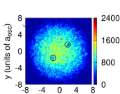
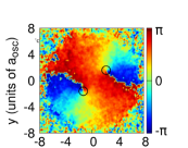
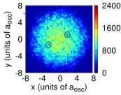
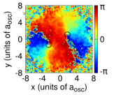
Figure 4: (Color online) The density (left column) and phase profiles (right column) of the condensate with two corotating vortices just before switching of the rotational frequency at $T=30$ nK (upper panel) and $40$ nK (lower panel). The locations of the vortices have been marked by two black circles in each image.

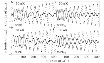
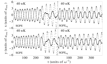
Figure 5: The $x$- and $y$-coordinates of the vortices as a function of time at $30$ nK and $40$ nK temperatures. It can be seen that there is an asymmetry in decay rates that increases with time.

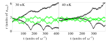
Figure 6: The black dots are the radial coordinates of the vortices as a function of time at $30$ nK and $40$ nK temperatures obtained using SGPE method. The green dots are the radial coordinates of the vortices obtained using GP equation with $N=1.3\times 10^{5}$ and $1.4\times 10^{5}$ for the left and right figures respectively.

In order to delineate the role of the these two processes, let us look at the $T=0$ dynamics of two corotating vortices intially located at unequal radial distances. In order to do so, we first generate the vortex pair by imprinting the corresponding phase singularities at each (imaginary) time step while evolving Eq. (1) in imaginary time, i.e., change

$$\Phi\rightarrow|\Phi|\exp\left\{i\left[\tan^{-1}\left(\frac{y-y_{1}}{x-x_{1}}\right)+\tan^{-1}\left(\frac{y-y_{2}}{x-x_{2}}\right)\right]\right\}$$

after each time step. Here $(x_{1},y_{1})$ and $(x_{2},y_{2})$ are the locations of two vortices and are chosen to be equal to the locations of vortices at $30$ nK and $40$ nK just prior to switching off $\Omega$. The number of atoms is fixed to $1.3\times 10^{5}$ and $1.4\times 10^{5}$ for the case corresponding to $30$ nK and $40$ nK respectively. This solution is then evolved in real time again using Eq. (1). We observe that the two vortices rotate about the trap center with their respective radial coordinates oscillating with time. This is shown in Fig. 6 with green dots. We find that due to these oscillations in the radial coordinates at $T=0$ K, the two vortices alternatively end up being located at farther distance from the trap center as is evidenced by green dots in Fig. 6. The amplitude of these oscillations in the radial coordinates is more for more assymetry in thier initial locations. Now, at finite temperatures, due to ocillating radial coordinates of the vortices during the intial stages of the evolution (the period during which the dynamics of the vortices will be qualitatively similar to $T=0$ dynamics), the random thermal fluctuations will result in one of the vortices decaying slightly faster than the other. While this vortex moves away from the trap center, the other vortex moves closer the trap center, reminiscent of their dynamics at $T=0$ K, due to the combined affect processes (a) and (b). As is the case at $T=0$ K, the radial coordinates of the two vortices show an anticorrelated behaviour, i.e, when one is moving away from the trap center, the other is moving towards it. Hence, the combined effect of the processes (a), (b), and (c) results in a positive feedback whereby the rate of decay of the slower decaying vortex is suppressed and that of the faster decaying one is enhanced. The faster decaying vortex is removed quickly from the system, after which the second vortex will decay like a single isolated vortex.

IV.2 Dynamics of a vortex dipole

Rotating the trapping potential can only lead to the formation of co-rotating vortices. Hence, we need an alternative method to create the vortex-antivortex pairs (vortex dipoles). It has been established both theoretically and experimentally that when a superfluid moves past an impurity faster than a critical speed, vortex dipoles are generated Frisch ; Neely . In the present work, we create a vortex dipole in the BEC by moving a Gaussian obstacle potential across it above a critical speed. Recently, the method was also used by us to study the generation and stability of vortex-bright soliton dipoles in phase-separated binary condensates Gautam-1 . In our simulations, we first generate the stationary solution without the obstacle potential, i.e., only in the presence of a harmonic trapping potential. Then, we slowly introduce the obstacle potential, keeping it fixed at a point. This procedure ensures that no phase singularity is trapped by the obstacle potential. In the present work, we consider $10^{5}$-$1.5\times 10^{5}$ atoms of ⁸⁷Rb (the exact number is a function of temperature) trapped in a trapping potential with $\omega=\omega_{x}=\omega_{y}=2\pi\times 10$ Hz and $\omega_{z}=2\pi\times 100$ Hz. In addition to this, there is a Gaussian obstacle potential

$$V_{\rm obs}=V_{0}e^{\frac{-2\{(x-x_{0}(t))^{2}+y^{2}\}}{w_{0}^{2}}},$$ (11)

where $(x_{0},0)$ is the location of the obstacle potential, $V_{0}$ its amplitude, and $w_{0}$ its width. In the present work $x_{0}(0)=-4~{}a_{\rm osc}$, $V_{0}=100~{}\hbar\omega_{x}$ and $w_{0}=2.5~{}\mu$m. The critical speed for these set of parameters at $1$ fK is $\sim 360~{}\mu$m/s. The density profiles of the condensate obtained by using this set of parameters at $1$ fK, $1$ nK and $10$ nK are shown in the upper row of Fig. 7.

Figure 7: (Color online) The upper row shows the density distribution of the condensate with the obstacle potential at $-4~{}a_{\rm osc}$. The left, middle and right images are at $T=1$ fK, $1$ nK, and $10$ nK, respectively. The bottom row shows the density distribution after $t=3.659537~{}\omega^{-1}$.

In order to generate the vortex dipole, the obstacle is moved along the $x$-axis at an optimum speed. As the obstacle is moved, its strength is continuously decreased so that the obstacle potential vanishes at $x=4~{}a_{\rm osc}$. We observe that at sufficiently low temperatures, the vortices are generated symmetrically about the $x-$axis, but not at higher temperatures (see images in the lower row of Fig. 7). This asymmetry in the generation of vortex-antivortex pairs was also pointed by us in an earlier work Prabhakar . The asymmetry in location of the vortex and antivortex has also been observed experimentally as is evident from the inset of Fig. 2 in Ref. Neely . Due to this asymmetry, the trajectory of a vortex dipole at higher temperatures is qualitatively different from near zero temperatures (say of the order of a few fK) as is shown in Fig .8.

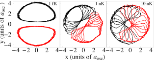
Figure 8: (Color online) Trajectories of the vortex dipole at $1$ fK, $1$ nK, and $10$ nK temperatures. The black and red colors correspond to vortex and antivortex respectively. The obstacle is moving at a speed of $380~{}\mu$m/s. The trajectories have been tracked for a period of $\approx 310~{}\omega^{-1}$.

We have employed both the SGPE_eq and SGPE to study vortex dipole generation and its dynamics at $1$ nK, $10$ nK, $30$ nK and $40$ nK. As in the case of a single vortex, we find that the results obtained with two methods are in good agreement during the initial period of evolution at all temperatures as shown in Fig. 9. Also evident from the Fig. 9 is that as the temperature is increased the vortex dipole decays faster. In fact at $40$ nK, the vortex dipole has already decayed before $t=300~{}\omega^{-1}$ as shown in Fig. 9. We find that at lower temperatures of $1$ nK, $10$ nK, and $30$ nK, the component vortices of the dipole decay at approximately same rate. At $40$ nK temperature, the component vortices decay at slightly different rate. As a result of it, the vortex (represented by solid-blue curve in Fig. 9) is ejected out of the condensate earlier than the antivortex (represented by solid-grey curve in Fig. 9). The roughly similar rate of decay of the vortex and antivortex is due to the attractive interaction between them, in contrast to the case of the two co-rotating vortices, where the interaction is repulsive. In the case of the dipole, a negative feedback that tends to oppose any asymmetry in the decay rate between the vortex and antivortex since the elimination of only one tends to increase the energy of the system. Thus, both tend to decay at roughly the same rate with the asymmetry becoming more pronounced at higher temperature as the strength of thermal fluctuations (responsible for the asymmetry) increases.

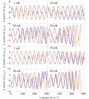
Figure 9: (Color online) Vortex dipole dynamics at $1$, $10$, $30$ and $40$ nK. The solid curves correspond to results obtained using the SGPE while the dotted and dashed curves correspond to the results obtained using the SGPE_eq. Solid-blue and dashed-orange curves represent the dynamics of the vortex and solid-grey and dotted-red represent the dynamics of antivortex.

The variation in the number of atoms after the obstacle starts moving is shown in Fig. 10.

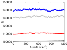
Figure 10: (Color online) The plot shows the number of atoms as function of time, obtained using SGPE, after the obstacle starts moving. The black, red, grey and blue curves correspond to $1$, $10$, $30$, and $40$ nK respectively. In the SGPE_eq, the number remains fixed to the value at $t=0$ at all temperatures.

V Summary and conclusions

We have studied the dynamics of a single and a pair of vortices in quasi two-dimensional systems at finite temperatures using the SGPE and SGPE_eq methods. These methods describe BECs well in the regime where thermal fluctuations are significantly high. We find that like a single vortex, a pair of vortices tends to decay as the system evolves. The rate of decay depends upon the temperature and the initial location of the constituent vortices. We find that on shorter time scales the dynamics of the system is basically governed by the multi-mode order parameter, which represents a few highly occupied low lying modes. For this reason, the results of the SGPE_eq, which governs the intrinsic evolution of the multimode order parameter, agree with those obtained from the SGPE during this period. The higher modes affect the dynamics of the system on longer time scales. For a pair of vortices, the two vortices are not symmetrically generated with respect to each other. In the case of corotating vortices, this initial asymmetry in their generation, coupled with random thermal fluctuations and a positive feedback resulting from the repulsive interaction between them leads to different decay rates for the two vortices. In contrast, the component vortices of a dipole decay at approximately same rate due to a negative feedback arising from the attractive interaction between them. At higher temperatures where thermal fluctuations are stronger, the asymmetry in the decay rates gets more pronounced.

- (1) M. R. Matthews, B. P. Anderson, P. C. Haljan, D. S. Hall, C. E. Wieman, and E. A. Cornell, Phys. Rev. Lett. 83, 2498 (1999).
- (2) K. W. Madison, F. Chevy, W. Wohllenben, and J. Dalibard, Phys. Rev. Lett. 84, 806 (2000); K. W. Madison, F. Chevy, V. Bretin, and J. Dalibard, Phys. Rev. Lett. 86, 4443 (2001).
- (3) C. Raman, J. R. Abo-Shaeer, J. M. Vogels, K. Xu, and W. Ketterle, Phys. Rev. Lett. 87, 210402 (2001).
- (4) J. R. Abo-Shaeer, C. Raman, J. M. Vogels, and W. Ketterle, Science 292, 476 (2001).
- (5) A. .E. Leanhardt, A. Görlitz, A. P. Chikkatur, D. Kielpinski, Y. Shin, D. E. Pritchard, and W. Ketterle, Phys. Rev. Lett. 89, 190403 (2002).
- (6) T. W. Neely, E. C. Samson, A. S. Bradley, M. J. Davis, and B. P. Anderson, Phys. Rev. Lett. 104, 160401 (2010).
- (7) B. P. Anderson, P. .C. Haljan, C. A. Regal, D. L. Feder, L. A. Collins, C. W. Clark, and E. A. Cornell, Phys. Rev. Lett. 86, 2926 (2001).
- (8) C. Weiler, T. W. Neely, D. R. Scherer, A. .S. Bradley, M. J. Davis, and B. P. Anderson, Nature 455, 948 (2008).
- (9) D. V. Freilich, D. M. Bianchi, A. M. Kaufman, T. K. Langin, D. S. Hall, Science 329, 1182 (2010).
- (10) S. Middelkamp, P. J. Torres, P. G. Kevrekidis, D. J. Frantzeskakis, R. Carretero-González, P. Schmelcher, D. V. Freilich, and D. S. Hall, Phys. Rev. A 84, 011605(R) (2011).
- (11) P. J. Torres, P. G. Kevrekidis, D. J. Frantzeskakis, R. Carretero-González, P. Schmelcher, D. S. Hall, Phys. Lett. A 375, 3044 (2011).
- (12) R. Navarro, R. Carretero-González, P. J. Torres, P. G. Kevrekidis, D. J. Frantzeskakis, M. W. Ray, E. Altuntas, and D. S. Hall, Phys. Rev. Lett. 110, 225301 (2013).
- (13) H. Schmidt, K. Góral, F. Floegel, M. Gajda, and K. Rzazewski, J. Opt. B: Quantum Semiclass. Opt. 5 S96, (2003).
- (14) E. J. Madarassy and C. F. Barenghi, J. Low Temp. Phys. 152, 122 (2008).
- (15) B. Jackson, N. P. Proukakis, C. F. Barenghi, and E. Zaremba, Phys. Rev. A 79, 053615 (2009).
- (16) A. J. Allen, E. Zaremba, C. F. Barenghi, and N. P. Proukakis, Phys. Rev A 87, 013630 (2013).
- (17) T. M. Wright, A. .S. Bradley, and R. J. Ballagh, Phys. Rev. A 80, 053624 (2009).
- (18) S. J. Rooney, A. S. Bradley, and P. B. Blakie, Phys. Rev. A 81, 023630 (2010).
- (19) H. T. C. Stoof, J. Low Temp. Phys. 114 11 (1999).
- (20) R. A. Duine and H. T. C. Stoof, Phys. Rev. A 65, 013603 (2001).
- (21) H. T. C. Stoof and M. J. Bijlsma, J. Low Temp. Phys. 124, 431 (2001).
- (22) R. .A. Duine, B. W. A. Leurs, and H. T. C. Stoof, Phys. Rev. A 69, 053623 (2004).
- (23) N. P. Proukakis, Phys. Rev. A 74, 053617 (2006).
- (24) S. P. Cockburn and N. P. Proukakis, Laser Physics 19, 558 (2009).
- (25) S. P. Cockburn, H. E. Nistazakis, T. P. Horikis, P. G. Kevrekidis, N. P. Proukakis, and D. J. Frantzeskakis, Phys. Rev. Lett. 104, 174101 (2010).
- (26) S. P. Cockburn, H. E. Nistazakis, T. P. Horikis, P. G. Kevrekidis, N. P. Proukakis, and D. J. Frantzeskakis, Phys. Rev. A 84, 043640 (2011).
- (27) S. P. Cockburn, A. Negretti, N. P. Proukakis, and C. Henkel, Phys. Rev A 83, 043619 (2011).
- (28) S. P. Cockburn and N. P. Proukakis, Phys. Rev. A 86, 033610 (2012).
- (29) F. Dalfovo, S. Giorgini, L. P. Pitaevskii, and S. Stringari, Rev. Mod. Phys. 71, 463–512 (1999).
- (30) W. Bao, D. Jaksch, and P. A. Markowich, J. Comp. Phys. 187, 318 (2003).
- (31) P. B. Blakie, A. S. Bradley, M. J. Davis, R. J. Ballagh, and C. W. Gardiner, Adv. Phys. 57, 363 (2008).
- (32) C. W. Gardiner, J. R. Anglin, and T. I. A. Fudge, J. Phys. B 35, 1555 (2002).
- (33) C. W. Gardiner and M. J. Davis, J. Phys. B 36, 4731 (2003).
- (34) N. P. Proukakis, J. Schmiedmayer, and H. T. C. Stoof, Phys. Rev. A 73, 053603 (2006).
- (35) M. J. Steel, M. K. Olsen, L. I. Plimak1, P. D. Drummond, S. M. Tan, M. J. Collett, D. F. Walls, and R. Graham, Phys. Rev. A 58, 4824–4835 (1998).
- (36) V. Bagnato and D. Kleppner, Phys. Rev. A 44, 7439 (1991).
- (37) M. Holzmann, M. Chevallier, and W. Krauth, Euro. Phys. Lett. 82, 30001 (2008).
- (38) A. A. Penckwitt, R. J. Ballagh, and C. W. Gardiner, Phys. Rev. Lett. 89, 260402 (2002).
- (39) T. Frisch, Y. Pomeau, and S. Rica, Phys. Rev. Lett. 69, 1644 (1992).
- (40) S. Gautam, P. Muruganandam, and D. Angom, J. Phys. B 45, 055303 (2012); S. Gautam, P. Muruganandam, and D. Angom, Phys. Lett. A 377, 378 (2013).
- (41) S. Prabhakar, R. P. Singh, S. Gautam, and D Angom, J. Phys. B: At. Mol. Opt. Phys. 46, 125302 (2013).